$z\sim 2-9$ Galaxies magnified by the Hubble Frontier Field Clusters II: Luminosity Functions and Constraints on a Faint End Turnover

Abstract

We present new determinations of the rest-UV luminosity functions (LFs) at $z=2$-9 to extremely low luminosities ($>$$-$14 mag) from a sample of $>$2500 lensed galaxies found behind the HFF clusters. For the first time, we present faint-end slope results from lensed samples that are fully consistent with blank-field results over the redshift range $z=2$-9, while reaching to much lower luminosities than possible from the blank-field studies. Combining the deep lensed sample with the large blank-field samples allows us to set the tight constraints on the faint-end slope $\alpha$ of the $z=2$-9 UV LFs and its evolution. We find a smooth flattening in $\alpha$ from $-$2.28$\pm$0.10 ($z=9$) to $-$1.53$\pm$0.03 ($z=2$) with cosmic time (d$\alpha$/dz$=$$-$0.11$\pm$0.01), fully consistent with dark matter halo buildup. We utilize these new results to present new measurements of the evolution in the $UV$ luminosity density $\rho_{UV}$ brightward of $-$13 mag from $z\sim 9$ to $z\sim 2$. Accounting for the SFR densities to faint luminosities implied by our LF results, we find that unobscured star formation dominates the SFR density at $z\gtrsim 4$, with obscured star formation dominant thereafter. Having shown we can quantify the faint-end slope $\alpha$ of the LF accurately with our lensed HFF samples, we also quantify the apparent curvature in the shape of the UV LF through a curvature parameter $\delta$. The constraints on the curvature $\delta$ strongly rule out the presence of a turn-over brightward of $-$13.1 mag at $z\sim 3$, $-$14.3 mag at $z\sim 6$, and $-$15.5 mag at all other redshifts between $z\sim 9$ to $z\sim 2$.

1. Introduction

One key frontier in extragalactic astronomy is the study of lower luminosity faint galaxies in the early universe. Lower luminosity galaxies in the $z\geq 3$ universe are the plausible progenitors to several different variety of stellar systems in the nearby universe. This has included both dwarf galaxies (Weisz et al. 2014; Boylan-Kolchin et al. 2015) and globular clusters (Bouwens et al. 2017a,c; Bouwens et al. 2021b; Vanzella et al. 2017a,b, 2019, 2020). Through resolved stellar population analyses and abundance matching, it is possible to set constraints on the form of the $UV$ LF at $z\geq 2$ (Weisz et al. 2014; Boylan-Kolchin et al. 2015), with evidence found for there being a flattening in the $UV$ LF faintward of $-13$ mag at $z\sim 7$ (Boylan-Kolchin et al. 2015).

Characterization of lower luminosity galaxies can give us insight into the efficiency of star formation in very low mass galaxies in the universe. There has been significant debate on whether this efficiency evolves with cosmic time since an influential analysis by Behroozi et al. (2013), with some studies favoring efficient early star formation (e.g., Harikane et al. 2016; Marrone et al. 2018) and others disfavoring it (e.g., Harikane et al. 2018, 2021; Stefanon et al. 2021, 2022). Lensed galaxies behind the HFF clusters allow for a direct look into what the efficiency of star formation is in low mass galaxies either from a direct look at the $UV$ LF (e.g., Muñoz & Loeb 2011; Finlator et al. 2017), the star-forming main sequence (Santini et al. 2018), galaxy stellar mass function (Bhatawdekar et al. 2019; Kikuchihara et al. 2020; Furtak et al. 2021), or evolution of the star-formation rate density itself to $z\sim 9$-10 (Oesch et al. 2015, 2018a; McLeod et al. 2016; Ishigaki et al. 2018; Bhatawdekar et al. 2019). Insight into the star formation efficiency of the lowest mass systems at $z\sim 7$-8 provide us with clues regarding similar star formation processes in galaxies at the earliest times ($z\geq 12$: Wise et al. 2014; Barrow et al. 2017; Harikane et al. 2021), while also constraining the nature of dark matter (e.g., Dayal et al. 2017; Menci et al. 2018).

Finally, lower luminosity galaxies have long been speculated to provide an important contribution to cosmic reionization (e.g., Bunker et al. 2004; Yan & Windhorst 2004; Bouwens et al. 2007; Ouchi et al. 2009; Robertson et al. 2013; Atek et al. 2015; Livermore et al. 2017; Bouwens et al. 2017b). As such, there has been great interest in quantifying their prevalence in the $z\geq 6$ universe as well as the escape fraction in these systems and their Lyman-continuum production efficiency (e.g., Lam et al. 2019; Robertson 2021). These lower luminosity galaxies are likely important contributors to the ionizing flux at early times. For LFs with a faint-end slope of $-$2, similar to what is observed at $z\geq 6$, and a turn-over in the LF faintward of $-$12 mag, $\geq$50% of the ionizing photons arise from galaxies fainter than $-$16.5 mag (e.g., Bouwens 2016). Yet $-$16.5 mag is as faint as one can probe at $z\geq 6$ in deep fields like the Hubble Ultra Deep Field (e.g., Schenker et al. 2013; McLure et al. 2013; Bouwens et al. 2015a, 2021a; Finkelstein et al. 2015).

The entire enterprise of directly searching for extremely low luminosity galaxies in the early universe took a major step forwards with the planning and execution of the ambitious 840-orbit Hubble Frontier Fields campaign (Coe et al. 2015; Lotz et al. 2017). This campaign combined the power of very long exposures with the Hubble Space Telescope with gravitational lensing from massive galaxy clusters to probe to unprecedented flux levels in the distant universe. Sensitive optical and near-IR observations were obtained of six clusters and six parallel fields, and soon complemented by observations in the near-UV with WFC3/UVIS (Alavi et al. 2016), in the K-band with HAWK-I/MOSFIRE (Brammer et al. 2016), in the mid-IR with Spitzer/IRAC (Capak et al. 2022, in prep) as well as near-IR grism observations (Schmidt et al. 2014) and optical spectroscopy with MUSE (Karman et al. 2015; Caminha et al. 2016; Mahler et al. 2018).

There were immediate attempts to take advantage of the great potential of deep HST observations over lensing clusters to probe the faint end of the $UV$ luminosity functions (LFs) at high redshift. In some early pioneering work, constraints were set on the prevalence of lower-luminosity $z\sim 6$-7 galaxies to $-$15 mag (Atek et al. 2014, 2015a, 2015b; Coe et al. 2015; Ishigaki et al. 2015; Laporte et al. 2016) and on lower luminosity $z\sim 2$ galaxies to $-$13 mag (Alavi et al. 2014, 2016). Later work on the HFF clusters identified plausible $z\sim 6$-7 sources to $-$13 mag (Kawamata et al. 2015; Castellano et al. 2016; Livermore et al. 2017; Yue et al. 2018; Atek et al. 2018; Kawamata et al. 2018), while also deriving constraints on the faint-end slope $\alpha$ (Atek et al. 2015a, 2015b, 2018; Ishigaki et al. 2015, 2018; Livermore et al. 2017; Bouwens et al. 2017b; Bhatawdekar et al. 2019) as well as a possible cut-off at very faint magnitudes (Castellano et al. 2016; Livermore et al. 2017; Bouwens et al. 2017b; Yue et al. 2018; Atek et al. 2018).

Despite the great potential of the HFFs for characterizing the faintest observable galaxies, the actual process of using lensing magnification to characterize the faint end ($>$$-$16 mag) of the $UV$ LF is challenging, due to the impact of systematic errors on the faint-end form of the $UV$ LF. One of these sources of error is the size (or surface brightness) distribution assumed for the faintest high-redshift sources (Bouwens et al. 2017a; Atek et al. 2018). This issue is important for quantifying the prevalence of faint galaxies due to the impact of source size on their detectability (Grazian et al. 2011; Bouwens et al. 2017a). The issue was appreciated to be especially important at the faint end due to the surface brightness of star-forming galaxies scaling as the square root of the luminosity for standard size-luminosity relations (Huang et al. 2013; Shibuya et al. 2015), such that 0.001 $L^{*}$ galaxies would have surface brightnesses $\sim$30$\times$ lower than for $L^{*}$ galaxies (Bouwens et al. 2017a, 2017b).

A second major source of error are uncertainties in the lensing models themselves and the impact this has on $UV$ LF results (Bouwens et al. 2017b; Atek et al. 2018). Comparisons of different lensing models can show a wide range in the predicted magnifications for individual sources ($\sim$0.3-0.5 dex scatter), with the position of high magnification critical lines varying by $\lesssim 1^{\prime\prime}$ from one model to another (Meneghetti et al. 2017; Sebesta et al. 2016; Bouwens et al. 2017b, 2022b). The magnification factors for sources in the highest-magnification regions are accordingly the most uncertain and can have a particularly large impact on the recovered $UV$ LF. The uncertainties are sufficient to completely wash out a turn-over at the faint-end of the LF (Bouwens et al. 2017b).

Fortunately, significant progress has been made over the last few years, allowing us to largely overcome the aforementioned challenges. Detailed quantitative analyses of the rest-$UV$ sizes of the faintest and highest magnification sources (Bouwens et al. 2017a,c, 2022a; Kawamata et al. 2018; Yang et al. 2022) indicate that the rest-$UV$ sizes of galaxies are much smaller than one would expect based on extrapolation from standard size luminosity relations (Huang et al. 2013; Shibuya et al. 2015). The small sizes of faint sources result in substantially smaller completeness correction than if these sources were more extended (Bouwens et al. 2017b, 2022a; Kawamata et al. 2018). Similarly, use of the median magnification from multiple public lensing models (Livermore et al. 2017; Bouwens et al. 2017b; Bhatawdekar et al. 2019; Bouwens et al. 2022b) and forward modeling (Bouwens et al. 2017b; Atek et al. 2018) provide us with a very effective way of accounting for the uncertainties in lensing models for specific clusters. By creating mock data sets on the basis of candidate LFs and specific lensing models and interpreting the observations using a median of the other magnification maps, one can replicate the LF recovery process and arrive at realistic uncertainties on the overall shape of the recovered LF. This is illustrated both by Bouwens et al. (2017b) and by Atek et al. (2018).

Making use of these advances, Bouwens et al. (2017b) were able to leverage the HFF data and derive faint-end slopes to the $UV$ LF at $z\sim 6$ which were completely consistent with blank-field LF results (e.g., Bouwens et al. 2015a). This was an important result, given significant long standing concerns about the impact of systematic uncertainties on such measurements (e.g., Bradač et al. 2009; Bouwens et al. 2009b; Maizy et al. 2010).

Table 1Samples of $z=2$-10 Galaxies found over the six HFF cluster fields (including the Oesch et al. 2018a $z\sim 10$ selection)

Cluster	Area [arcmin2]	$z\sim 2$	$z\sim 3$	$z\sim 4$	$z\sim 5$	$z\sim 6$	$z\sim 7$	$z\sim 8$	$z\sim 9$	$z\sim 10$
Abell 2744	4.9	157	233	—	27	49	25	15	4	2
MACS0416	4.9	215	233	—	7	50	26	10	6	0
MACS0717	4.9	81	160	32	—	26	14	9	0	0
MACS1149	4.9	134	195	36	—	52	21	5	2	0
Abell S1063	4.9	96	203	—	11	62	28	6	3	0
Abell 370	4.9	82	152	—	14	35	11	6	1	0
Total	29.4	765	1176	68	59	274	125	51	16	2

With a demonstration of the effectiveness of the approach we pioneered in Bouwens et al. (2017b) for characterizing the faint end of the $UV$ LF at $z\sim 6$, the next step is to apply this metholodogy to the galaxies over a wider redshift range to derive the relevant LFs. It is the purpose of this study to derive such a set of LFs and do it over the redshift range $z=2$-9 where star-forming galaxies can be readily identified in the distant universe. Additionally, we will characterize the evolution of the faint-end slope $\alpha$ as well as any potential turn-over at the extreme faint end of each LF. Mapping out the extreme faint end of the UV LF is valuable for providing insight into the efficiency of star formation in lower mass galaxies and quantifying the total budget of ionizing photons available at $z\geq 6$ to drive cosmic reionization. For this effort, we make use of the extremely large $>$2500-source sample of lensed galaxies recently identified at $z\sim 2$-9 over all six HFF clusters in a companion paper (Bouwens et al. 2022b).

Here we provide a brief outline of our plan for this manuscript. In §2, we begin by reviewing the primary data sets we utilize and describing the basic properties of our selected high-redshift samples. §3 details our procedure for deriving the LF from the lensing clusters and describes our basic LF results. In §4, we compare our new results with previous work in the literature and consider the scientific implications of our new results. Finally, in §5, we include a summary. For consistency with our previous work, results will frequently be quoted in terms of the luminosity $L_{z=3}^{*}$ Steidel et al. (1999) derived at $z\sim 3$, i.e., $M_{1700,AB}=-21.07$. The HST F275W, F336W, F435W, F606W, F814W, F105W, F125W, F140W, and F160W bands are referred to as $UV_{275}$, $U_{336}$, $B_{435}$, $V_{606}$, $I_{814}$, $Y_{105}$, $J_{125}$, $JH_{140}$, and $H_{160}$, respectively, for simplicity. Where necessary, $\Omega_{0}=0.3$, $\Omega_{\Lambda}=0.7$, and $H_{0}=70\,\textrm{km/s/Mpc}$ is assumed. All magnitudes are in the AB system (Oke & Gunn 1983).

2. Data Sets and High-Redshift Samples

2.1. Data Sets

We will base the present deep LF results primarily on the sensitive near-UV, optical, and near-IR observations obtained by the HFF program (Coe et al. 2015; Lotz et al. 2017) and a follow-up GO campaign of the HFF clusters with WFC3/UVIS (Alavi et al. 2014, 2016; Siana 2013, 2015). Over each of the six clusters in the HFF program, at least 16 orbits of WFC3/UVIS time (8 and 8 in the $UV_{275}$ and $U_{336}$ bands), 70 orbits of optical ACS time (18, 10, and 42 in the $B_{435}$, $V_{606}$, and $I_{814}$ bands), and 70 orbits of WFC3/IR time (24, 12, 10, and 26 in the $Y_{105}$, $J_{125}$, $JH_{140}$, and $H_{160}$ bands) was invested into observations of each cluster, with additional observations coming from the CLASH (Postman et al. 2012) and GLASS (Schmidt et al. 2014) programs. We made use of the v1.0 reductions of these observations made publicly available by the HFF team (Koekemoer et al. 2014). For the WFC3/UVIS observations, we made our own reductions, following similar procedures to what we utilized in reducing the UVIS observations obtained as part of the HDUV program (Oesch et al. 2018b).

In addition, we will make use of the $z=2$-9 LF constraints available from the comprehensive set of blank-field HST observations recently utilized by Bouwens et al. (2021a). For that analysis, Bouwens et al. (2021a) not only made use of the extremely sensitive optical, near-IR, and rest-UV observations obtained over the Hubble Ultra Deep Field (Beckwith et al. 2006; Koekemoer et al. 2013; Illingworth et al. 2013; Teplitz et al. 2013), but also made use of the sensitive ultraviolet, optical, and near-IR data over the five CANDELS fields and ERS field (Grogin et al. 2011; Koekemoer et al. 2011; Oesch et al. 2018b), Hubble Frontier Field parallels (Coe et al. 2015; Lotz et al. 2016), and pure parallel search fields (Trenti et al. 2011; Yan et al. 2011).

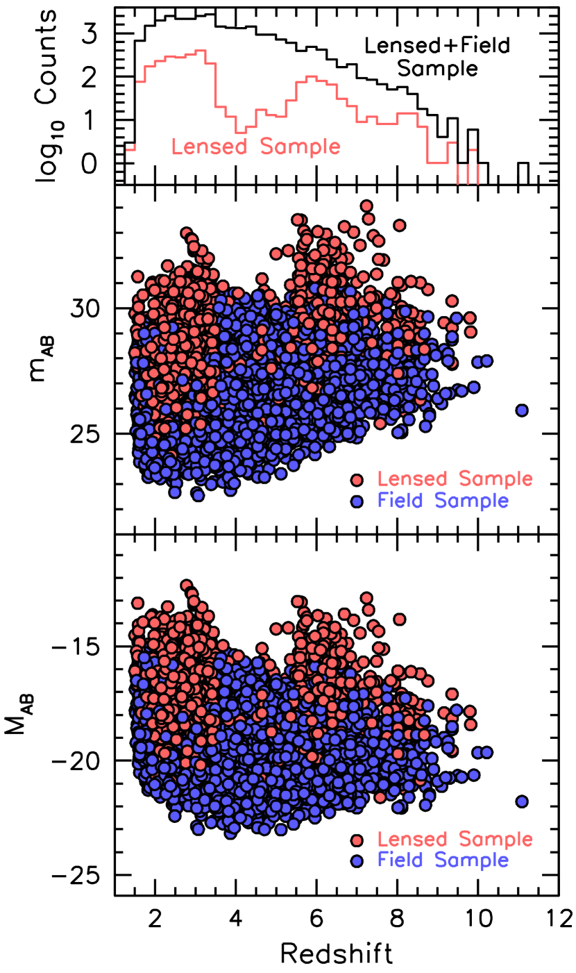
Figure 1.— (upper) The number of sources per unit redshift (shown in logarithmic units) in our lensed sample constructed from the HFF ’cluster’ fields (light red histogram) and this sample combined with the Bouwens et al. (2021a) blank-field sample (black histogram). (middle panel) The distribution of sources in apparent magnitude and redshift from our HFF ’cluster’ fields (red circles: Bouwens et al. 2022b) and from an HST blank-field sample with $>$24000 sources (blue circles: Bouwens et al. 2021a). (lower) The distribution of sources in $UV$ luminosity and redshift from our HFF ’cluster’ fields (red circles) and from an HST blank-field sample (blue circles). It is clear that selections using lensing magnification can reach up to $\sim$10-40$\times$ fainter in luminosity than achieved using similar selections without the aide of lensing magnification. The relative paucity of $z\sim 4$-5 sources in our HFF ’cluster field’ selections relative to blank-field selections is a direct result of the very conservative selection criteria we impose at those two redshifts to minimize contamination from galaxies in the foreground clusters (see Figure 3 from Bouwens et al. 2022b).

2.2. Lensed Galaxy Samples at $z=2$-9

We consider the systematic application of $z=2$-9 Lyman-break galaxy selection criteria to the HFF near-UV, optical, and near-IR observations available over the six clusters that make up the HFF program. We describe our application of these criteria to the HFF observations in a companion paper (Bouwens et al. 2022b), and it is very similar to what we previously performed in Bouwens et al. (2015a, 2016a, and 2017b).

In total, we have identified 765, 1176, 68, 59, 274, 125, 51, and 16 sources as part of our $z\sim 2$, $z\sim 3$, $z\sim 4$, $z\sim 5$, $z\sim 6$, $z\sim 7$, $z\sim 8$, and $z\sim 9$ selections. The results are summarized in Table 1. $z\sim 4$ galaxies are exclusively selected around the two highest redshift clusters that make up the HFF program, i.e., MACS0717 and MACS1149. Meanwhile, $z\sim 5$ galaxies are selected behind the four lowest redshift clustes that make up the HFF program, i.e., Abell 2744, MACS0416, Abell S1063, and Abell 370. $z\sim 4$ and $z\sim 5$ selections are exclusively made behind these specific clusters to minimize contamination from foreground sources in clusters having spectral breaks at similar wavelengths to the breaks used to select Lyman-break galaxies. See Figures 2-4 from Bouwens et al. (2022b).

An illustration of the distribution of the present lensed sample in redshift and $UV$ magnitude is provided in Figure 1 along with the $>$24,000 source sample we utilize from the Bouwens et al. (2021a) blank-field selection. As should be apparent the lensed sample reaches $\sim$10-40$\times$ fainter in UV luminosity than does the blank-field sample, providing with much greater leverage for probing the faint-end form of the $z\geq 2$ LFs.

3. Luminosity Function Determinations

3.1. Basic Procedure

Here we describe our basic procedure for constraining the shape of the $UV$ LF for each of our intermediate to high redshift samples $z\sim 2$, $z\sim 3$, $z\sim 4$, $z\sim 5$, $z\sim 6$, $z\sim 7$, $z\sim 8$, and $z\sim 9$.

One significant challenge, in the derivation of the $UV$ LF results at high redshift from lensed samples, is the impact of errors in the estimated magnification factors for individual sources. As demonstrated in Bouwens et al. (2017b), errors in the magnification factors can effectively wash out faint-end ($>$$-$15 mag) turn-overs in the $UV$ LF, making it difficult to observationally test for the presence of such a turn-over in real-life observations.

We have already demonstrated in Bouwens et al. (2017b) how we can overcome the impact of potential errors in the lensing maps using a forward-modeling procedure (see Atek et al. 2018 for a separate approach using forward modeling). The basic idea is to leverage the availability of the many independent lensing models for each cluster to estimate the uncertainties. Model LFs are evaluated by treating one of the lensing maps as the truth and thus constructing a full catalog of observables with that map and then interpreting the observations using another lensing model. In this way, the expected number of sources per unit luminosity for a model LF could be realistically estimated. Figure 6 of Bouwens et al. (2017b) illustrates the basic procedure.

Here we will follow the same forward-modeling procedure as we introduced in Bouwens et al. (2017b). In evaluating model LFs, we treat one flavor of lensing model as the truth and use it to construct a complete catalog of background sources behind each cluster. Sources are added to a search field in proportion to the product of the model volume density, selection efficiency $S(m)$, and the cosmic volume element – which we take to be the cosmic volume element divided by the magnification factor. The selection efficiency $S$ is, in general, a function of both the apparent magnitude $m$ and the magnification factor $\mu$, but we can largely ignore the impact of magnification in the limit that faint sources have very small sizes. Justification for this is provided in the published results of Bouwens et al. (2017a), Kawamata et al. (2018), Bouwens et al. (2022a), and Bouwens et al. (2022b).

We then use a different lensing model to estimate the magnification factors and $UV$ luminosities for individual sources behind the cluster. To maximize the reliability of our results, we made use of the median magnification from the latest parametric lensing models for our fiducial LF determinations. Not only has use of the median magnification model been shown to provide robust estimates of the magnification to magnifications of $\gtrsim$50 (Livermore et al. 2017; Bouwens et al. 2017b, 2022a), but the parametric models were shown to best reproduce the input magnification models from the HFF comparison project (Meneghetti et al. 2017), with median differences ($<$0.1 dex differences) to magnification factors of 30. The parametric lensing models available for the HFF clusters and utilizing most of the public multiple image constraints, i.e., v3/v4, include the CATS (Jullo & Kneib 2009; Richard et al. 2014; Jauzac et al. 2015a,b; Lagattuta et al. 2017), Sharon (Johnson et al. 2014), GLAFIC (Oguri 2010; Ishigaki et al. 2015; Kawamata et al. 2016), Zitrin-NFW (Zitrin et al. 2013, 2015), and Keeton (2010) results. When computing the median magnification map used to estimate the magnification factors for our forward-modeling approach, any model we treat as the truth is naturally excluded.

While we base our fiducial LF results on the parametric lensing models available for the HFF clusters, we also derive LF results using the non-parametric lensing models available for the HFF clusters. The non-parametric lensing models have been shown to be a good match ($<$0.1 dex) to the input models from the HFF comparison project (Meneghetti et al. 2017) to magnification factors of $\sim$10-20. Given the greater flexibility of the non-parametric models relative to the parametric models, results derived from these models allow us to assess the impact lensing models have on our LF results.

We evaluate the likelihood of a LF model by comparing the observed number of sources in various absolute magnitude bins (0.5-mag width) with the expected number of sources assuming that galaxies are Poisson-distributed:

$${\cal L}=\Pi_{i}P_{i}$$

where

$$P_{i}=e^{-N_{exp,i}}\frac{(N_{exp,i})^{N_{obs,i}}}{(N_{obs,i})!}$$ (1)

$N_{obs,i}$ and $N_{exp,i}$ are the observed and expected number of sources in magnitude interval $i$. To reduce the impact of sources with complex multi-component or morphological structure on our analysis – which become common at the bright end of the LF – we only consider luminosity bins fainter than $-$19 mag. As a result of this choice, this analysis relies entirely on blank-field LF results for constraints brightward of $-$19 mag. Additionally, our forward-modeling simulations typically include $\sim$200$\times$ as many sources as are present in the actual observations (e.g., see Figure 6 from Bouwens et al. 2017b) to guarantee an accurate calculation of $N_{exp,i}$ for our likelihood estimates.

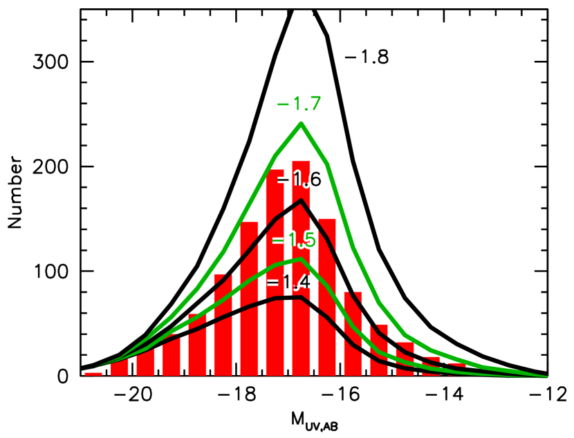
Figure 2.— Use of the lensed $z\sim 3$ samples from the HFF program (red histogram) to illustrate the leverage available to constrain the faint-end slope $\alpha$. The green and black lines show the predicted number of sources per bin for different values of the faint-end slope. The faint-end slope $\alpha$ appears to be $\sim$$-$1.65. Interestingly enough, we can use this figure to assess the faint-end slopes $\alpha$ derived earlier by Parsa et al. (2016) and Alavi et al. (2016), i.e., $-1.31\pm 0.04$ and $-1.94\pm 0.06$. Those results are strictly shallower and steeper, respectively, than the faint-end slopes for any of the models shown on this figure and thus appear to be inconsistent with our new results. Clearly, there is enormous leverage available in lensed HFF samples to constrain the faint-end slope very precisely (as also illustrated by the $\sim$2-3% uncertainties in $\alpha$ presented in Table 2).

To evaluate the likelihood of various LF parameters for our $z\sim 6$-9 samples, we must account for our combining five separate selections of $z\sim 6$, $z\sim 7$, $z\sim 8$, and $z\sim 9$ galaxies in creating our composite sample of $z\sim 6$-9 galaxies. This was done to maximize the utility of our results to constrain the faint end of the $z\sim 6$-9 LFs. Selections were constructed by leveraging a separate source catalog, each made with different parameters to handle the background parameters and thresholding (Bouwens et al. 2022b). While this results in a larger number of sources in each bin, many sources occur in our final catalog multiple times and are not independent. We can account for the impact of this by quantifying the fraction of sources $f_{i,j}$ in each bin $i$ that are counted $1\times$, $2\times$, $3\times$, $4\times$, and $5\times$ and assuming similar multiplicity fraction in the modeled statistics. As such, the probability $P_{i}$ for measuring a specific number of counts in bin $i$ is then the following:

$$P_{i}=\Sigma_{N_{obs,i,j}}\Pi_{j=1,5}e^{-f_{i,j}N_{exp,i}}\frac{(f_{i,j}N_{exp,i})^{N_{obs,i,j}}}{(N_{obs,i,j})!}$$ (2)

where the summation $\Sigma_{N_{obj,i,j}}$ runs over all $N_{obj,i,j}$ where the sum $\Sigma_{j=1,5}jN_{obj,i,j}$ is equal to $N_{obj,i}$. We have verified that Eq. 2 reduces to the appropriate Poissonian likelihood distribution in the limit that all sources are present in our catalogs with a fixed multiplicity (e.g., once or five times).

Due to the relatively modest depth of the $UV_{275}$ and $U_{336}$ data available to select our $z\sim 2$-3 samples, we only include sources brightward of 28.0 mag and 28.5 mag ($V_{606}$ and $I_{814}$ bands, respectively) to mitigate the impact of the uncertain completeness corrections faintward of these limits. For our $z\sim 4$ and $z\sim 5$ selections, where contamination from evolved galaxies at the redshift of the cluster is a particular concern, we restrict ourselves to using sources brightward of 27.3 and 27.5 mag, respectively.

We used extensive source recovery simulations to estimate selection efficiencies $S(m)$ for each of our intermediate to high-redshift samples. For each of the simulations, we first constructed mock catalogs of sources over the general redshift ranges spanned by each of our $z\sim 2$-9 samples, i.e., $z=1-4$, $z=1$-4, $z=2.5$-5.0, $z=4$-6, $z=5$-7, $z=5.5$-8, $z=6.5$-9.5, and $z=7$-10 for our $z\sim 2$, 3, 4, 5, 6, 7, 8, and 9 selections, respectively. We then created artificial two-dimensional images for each of the sources in these catalogs in all HST bands used for the selection and detection of the sources and then added these images to the real observations. We then repeated both our catalog creation procedure and source selection procedure in the same way as on the real observations (Bouwens et al. 2017a,b).

Motivated by our earlier findings regarding source sizes for faint $z\sim 2$-8 samples from the HFFs (Bouwens et al. 2017a; see also Kawamata et al. 2018; Bouwens et al. 2017c, 2022a; Yang et al. 2022), we adopted a point-source size distribution in modeling the completeness of sources over the HFFs for our fiducial LF results. Additionally, we took the $UV$-continuum slope $\beta$ distribution to a median value of $-2$ at $z\sim 2$-3, $-2.1$ at $z\sim 4$-5, and $-2.3$ at $z\sim 6$-8 consistent with the Kurczynski et al. (2014) and Bouwens et al. (2014) $UV$-continuum slope measurements. We have verified that for unlensed sources at the faint end of our HFF selections, we estimate almost identical selection volumes to what we estimate by computing the selection volumes using randomly-selected $z\sim 2$-4 galaxies as templates in our image simulations. We expect that this is due to the combination of the high surface brightness sensitivity of the HFF observations and the faintest sources in our fields having small sizes.

To quantify the possible systematic uncertainties that could result in our LF determinations from our size modeling, we have also repeated these completeness estimates using the size-luminosity relations of both Shibuya et al. (2015) and Bouwens et al. (2022a) to illustrate how large the systematic uncertainties could be, similar to the exercise we performed in §5.4 of Bouwens et al. (2017b). While we include these estimates as a possible systematic error on the derived faint-end LF results, we emphasize that this is a worst case scenario, as the results from Bouwens et al. (2017a), Kawamata et al. (2018), and Yang et al. (2022) results all point towards substantially smaller source sizes.

As an illustration of the substantial leverage available from the HFF samples to constrain the faint-end slope, we show in Figure 2 the number of sources behind the HFF clusters as a function of $UV$ luminosity and compare that to the predicted numbers for specific values for the faint-end slope of the $UV$ LF at $z\sim 3$. From this figure and substantial numbers of sources faintward of $-19$ mag, it is clear that the faint-end slope of the $z\sim 3$ LF must be fairly close to $-$1.63 and faint-end slopes of $-1.43$ and $-1.83$ can both be excluded at high confidence on the basis of the HFF results.

3.2. Functional Form and Optimization Procedure

As in Bouwens et al. (2017b), we adopt a standard Schechter functional form for our LF

$$\phi^{*}(\ln(10)/2.5)10^{-0.4(M-M^{*})(\alpha+1)}e^{-10^{-0.4(M-M^{*})}}$$

but modified to allow for curvature in the faint-end slope $\alpha$ at the faint end. We implement this using a new curvature parameter $\delta$ and multiply the standard Schechter form with the following expression faintward of $-$16 mag:

$$10^{-0.4\delta(M+16)^{2}}$$

As we demonstrate in Bouwens et al. (2017b), positive values of $\delta$ result in a turn-over in the LF at

$$M_{T}=-16-\frac{\alpha+1}{2\delta}$$ (3)

while negative values for $\delta$ result in the LF turning concave upwards.

Given our use of four separate parameters to characterize the overall shape of the $UV$ LF, we utilize a Markov-Chain Monte Carlo procedure both to determine the maximum likelihood value and to characterize the observational uncertainties. We begin the MCMC optimization process using the best-fit blank-field LF parameters from Bouwens et al. (2021a) and run $\sim$1000 iterations to find the best-fit LF parameters and map out the likelihood space.

3.3. LF Results at $z=2$-9

3.3.1 Leveraging Only Lensed Sources from the HFF Program

As in Bouwens et al. (2017b), we commence our analysis by exclusively making use of the lensed HFF samples to derive our initial $UV$ LF results. The value in doing this first is that it allows us to test for the presence of any systematic errors in lensing-cluster LF determinations vis-a-vis blank-field determinations. The two approaches have their own strengths and are subject to different sources of systematic error, so it is valuable to first look into this issue before combining the results to arrive the best constraints on the overall shape of the $UV$ LF.

In Bouwens et al. (2017b), we demonstrated we could obtain accurate constraints on both the faint-end slope $\alpha$ and $\phi^{*}$ at $z\sim 6$ relying only on the lensed $z\sim 6$ sources from the HFF lensing clusters. There, a faint-end slope $\alpha$ of $-1.92\pm 0.04$ and a $\phi^{*}$ of 0.66$\pm$0.06 $\times$ 10^-3 Mpc^-3 were found, consistent ($\lesssim$1$\sigma$) with the $-1.87\pm 0.10$ slope and 0.51${}_{-0.10}^{+0.12}$ $\times$ 10^-3 Mpc^-3 normalization found from blank-field observations (Bouwens et al. 2015a). For these determinations, the characteristic luminosity $M^{*}$ was fixed to $-$20.94 mag, the value obtained from wide-area blank-field studies, due to their being insufficient volume behind the HFF clusters to achieve strong constraints on this luminosity.

We adopt a similar approach here. We begin by fixing the characteristic luminosities $M^{*}$ for the $z\sim 2$-9 LFs to the values obtained by the Bouwens et al. (2021a) blank-field analysis and then use the described MCMC approach to identify the values of $\phi^{*}$, $\alpha$, and $\delta$ that maximizes the likelihood of recovering our $z\sim 2$-9 samples from the full HFF program. Uncertainties on the individual LF parameters can be calculated based on fits to the multi-dimensional likelihood surface derived from our MCMC simulations.

We present the LF results we derive using our lensed HFF samples and fixed values for the characteristic luminosity in Table 2. In addition, in Figure 3, we present our determinations of the faint-end slope $\alpha$ of the LF vs. redshift. A simple linear fit to the faint-end slope $\alpha$ results we derive vs. redshift yields the relation

$$\alpha=(-1.92\pm 0.03)+(-0.10\pm 0.01)(z-6)$$ (4)

and presented on Figure 3 as a blue line. For context, figure 3 also shows a recent determination of the faint-end slope $\alpha$ evolution based on blank-field observations alone (Bouwens et al. 2021a: red circles), with the observed trend with redshift (red line):

$$\alpha=(-1.92\pm 0.03)+(-0.11\pm 0.01)(z-6)$$ (5)

Encouragingly enough, the new faint-end slope $\alpha$ results we derive from lensing cluster observations seem very consistent (within the $1\sigma$ errors) both in terms of its slope and intercept with blank-field results over the entire redshift range we are examining $z\sim 2$ to $z\sim 9$.

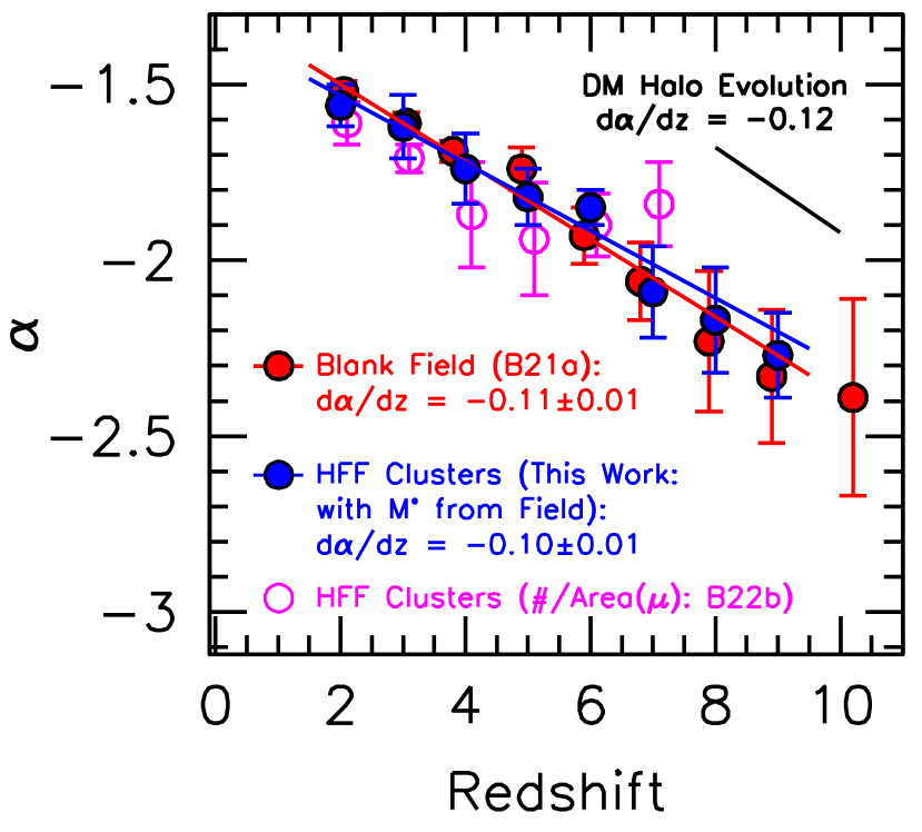
Figure 3.— Comparison of faint-end slope $\alpha$ determinations from lensed HFF galaxy samples (blue solid circles) with similar blank-field determinations of these slopes $\alpha$ (red solid circles: Bouwens et al. 2021a). The faint-end slope determinations shown here from the lensed HFF samples do not make use of any information from the blank-field search results, except for the value of characteristic luminosity $M^{*}$ (§3.3.1: but see Figure 6, Table 2, and §3.3.2 for $\alpha$ determinations using both the lensed HFF + blank-field constraints). The purple open circles are based on the surface density $\Sigma$ vs. magnification $\mu$ trend found in the companion paper (Bouwens et al. 2022b) for galaxies at $z\sim 2$, 3, 4, 5, 6, and 7. The blue and red lines show the essentially identical, and remarkable, best-fit evolution in the faint-end slope $\alpha$ from the lensing cluster and blank-field search results, respectively. This strongly suggests that there are minimal systematic errors in either determination, and that we can combine both probes to dramatically improve the statistical constraints on the evolution of the $UV$ LF and faint-end slope $\alpha$. This is the first time such agreement in the faint-end slope $\alpha$ evolution has been demonstrated over such a large range in redshift.

Table 2Summary of our Final Fiducial Constraints on the $z\sim 2$-9 $UV$ LFs

Data Sets + Method	$M_{UV}^{*}$	$\phi^{*}$ $(10^{-3}$ Mpc-3)	$\alpha$	$\delta$	$M_{T}$
$z\sim 2$
HFF + Blank-Field (Parametric, Fiducial)	$-$20.30$\pm$0.08	3.4$\pm$0.4	$-$1.53$\pm$0.03	0.09$\pm$0.11	$>$$-$15.2
HFF + Blank-Field (Non-Parametric)	$-$20.31$\pm$0.09	4.0$\pm$0.7	$-$1.53$\pm$0.03	0.20$\pm$0.13	$>$$-$15.3
HFF (Parametric) + $M^{*}$ Fixed	$-$20.28 (fixed)	3.0$\pm$0.6	$-$1.56$\pm$0.06	0.15$\pm$0.13
HFF (Parametric) + $M^{*}+\phi^{*}$ Fixed	$-$20.28 (fixed)	4.0 (fixed)	$-$1.49$\pm$0.03	0.05$\pm$0.11
$\Sigma(\mu)$ Fit			$\leq-1.61\pm 0.06$
Blank-Field (B21a)	$-$20.28$\pm$0.09	4.0${}_{-0.4}^{+0.5}$	$-$1.52$\pm$0.03	—
$z\sim 3$
HFF + Blank-Field (Parametric, Fiducial)	$-$20.84$\pm$0.07	2.3$\pm$0.4	$-$1.60$\pm$0.03	$-$0.06$\pm$0.05	$>$$-$13.1
HFF + Blank-Field (Non-Parametric)	$-$20.96$\pm$0.09	1.9$\pm$0.8	$-$1.65$\pm$0.04	0.05$\pm$0.07	$>$$-$12.3
HFF (Parametric) + $M^{*}$ Fixed	$-$20.87 (fixed)	2.0$\pm$1.5	$-$1.62$\pm$0.09	$-$0.03$\pm$0.06
HFF (Parametric) + $M^{*}+\phi^{*}$ Fixed	$-$20.87 (fixed)	2.1 (fixed)	$-$1.60$\pm$0.03	$-$0.06$\pm$0.04
$\Sigma(\mu)$ Fit			$\leq-1.71\pm 0.04$
Blank-Field (B21a)	$-$20.87$\pm$0.09	2.1${}_{-0.3}^{+0.3}$	$-$1.61$\pm$0.03	—
$z\sim 4$
HFF + Blank-Field (Parametric, Fiducial)	$-$20.93$\pm$0.07	1.6$\pm$0.3	$-$1.69$\pm$0.03	$-$0.18$\pm$0.18	$>$$-$15.3
HFF + Blank-Field (Non-Parametric)	$-$20.95$\pm$0.07	1.8$\pm$0.3	$-$1.71$\pm$0.03	$-$0.06$\pm$0.12	$>$$-$15.6
HFF (Parametric) + $M^{*}$ Fixed	$-$20.93 (fixed)	1.5$\pm$0.6	$-$1.71$\pm$0.09	$-$0.12$\pm$0.22
HFF (Parametric) + $M^{*}+\phi^{*}$ Fixed	$-$20.93 (fixed)	1.69 (fixed)	$-$1.68$\pm$0.05	$-$0.19$\pm$0.17
$\Sigma(\mu)$ Fit			$\leq-1.87\pm 0.15$
Blank-Field (B21a)	$-$20.93$\pm$0.08	1.69${}_{-0.20}^{+0.22}$	$-$1.69$\pm$0.03	—
Bouwens et al. (2007)	$-$20.98$\pm$0.10	1.3$\pm$0.2	$-$1.73$\pm$0.05	—
Bouwens et al. (2015a)	$-$20.88$\pm$0.08	1.97${}_{-0.29}^{+0.34}$	$-$1.64$\pm$0.04
$z\sim 5$
HFF + Blank-Field (Parametric, Fiducial)	$-$21.13$\pm$0.09	0.73$\pm$0.13	$-$1.78$\pm$0.04	$-$0.07$\pm$0.20	$>$$-$14.7
HFF + Blank-Field (Non-Parametric)	$-$21.15$\pm$0.10	0.74$\pm$0.14	$-$1.80$\pm$0.05	$-$0.02$\pm$0.24	$>$$-$14.8
HFF (Parametric) + $M^{*}$ Fixed	$-$21.10 (fixed)	0.66$\pm$0.15	$-$1.82$\pm$0.08	$-$0.03$\pm$0.21
HFF (Parametric) + $M^{*}+\phi^{*}$ Fixed	$-$21.10 (fixed)	0.79 (fixed)	$-$1.77$\pm$0.06	$-$0.07$\pm$0.20
$\Sigma(\mu)$ Fit			$\leq-1.94\pm 0.16$
Blank-Field (B21a)	$-$21.10$\pm$0.11	0.79${}_{-0.13}^{+0.16}$	$-$1.74$\pm$0.06	—
Bouwens et al. (2015a)	$-$21.17$\pm$0.12	0.74${}_{-0.14}^{+0.18}$	$-$1.76$\pm$0.05
$z\sim 6$
HFF + Blank-Field (Parametric, Fiducial)	$-$20.87$\pm$0.07	0.57$\pm$0.11	$-$1.87$\pm$0.04	0.05$\pm$0.10	$>$$-$14.3
HFF + Blank-Field (Non-Parametric)	$-$20.98$\pm$0.08	0.45$\pm$0.10	$-$1.98$\pm$0.06	0.36$\pm$0.18	$>$$-$15.2
HFF (Parametric) + $M^{*}$ Fixed	$-$20.93 (fixed)	0.61$\pm$0.29	$-$1.85$\pm$0.05	0.00$\pm$0.14
HFF (Parametric) + $M^{*}+\phi^{*}$ Fixed	$-$20.93 (fixed)	0.51 (fixed)	$-$1.87$\pm$0.02	0.09$\pm$0.09
$\Sigma(\mu)$ Fit			$\leq-1.90\pm 0.09$
Blank-Field (B21a)	$-$20.93$\pm$0.09	0.51${}_{-0.10}^{+0.12}$	$-$1.93$\pm$0.08	—
Bouwens et al. (2015a)	$-$20.94$\pm$0.20	0.50${}_{-0.16}^{+0.22}$	$-$1.87$\pm$0.10
$z\sim 7$
HFF + Blank-Field (Parametric, Fiducial)	$-$21.13$\pm$0.08	0.20$\pm$0.05	$-$2.05$\pm$0.06	0.24$\pm$0.20	$>$$-$15.2
HFF + Blank-Field (Non-Parametric)	$-$21.21$\pm$0.09	0.17$\pm$0.05	$-$2.13$\pm$0.07	0.56$\pm$0.26	$>$$-$15.4
HFF (Parametric) + $M^{*}$ Fixed	$-$21.15 (fixed)	0.17$\pm$0.12	$-$2.09$\pm$0.13	0.36$\pm$0.28
HFF (Parametric) + $M^{*}+\phi^{*}$ Fixed	$-$21.15 (fixed)	0.19 (fixed)	$-$2.06$\pm$0.04	0.25$\pm$0.16
$\Sigma(\mu)$ Fit			$\leq-1.84\pm 0.12$
Blank-Field (B21a)	$-$21.15$\pm$0.13	0.19${}_{-0.06}^{+0.08}$	$-$2.06$\pm$0.11	—
Bouwens et al. (2015a)	$-$20.87$\pm$0.26	0.29${}_{-0.12}^{+0.21}$	$-$2.06$\pm$0.13
$z\sim 8$
HFF + Blank-Field (Parametric, Fiducial)	$-$20.90$\pm$0.19	0.096$\pm$0.065	$-$2.20$\pm$0.09	0.23$\pm$0.28	$>$$-$15.2
HFF + Blank-Field (Non-Parametric)	$-$20.96$\pm$0.19	0.094$\pm$0.051	$-$2.27$\pm$0.09	0.50$\pm$0.30	$>$$-$15.3
HFF (Parametric) + $M^{*}$ Fixed	$-$20.93 (fixed)	0.11$\pm$0.09	$-$2.17$\pm$0.15	0.15$\pm$0.31
HFF (Parametric) + $M^{*}+\phi^{*}$ Fixed	$-$20.93 (fixed)	0.09 (fixed)	$-$2.21$\pm$0.05	0.32$\pm$0.17
Blank-Field (B21a)	$-$20.93$\pm$0.28	0.09${}_{-0.05}^{+0.09}$	$-$2.23$\pm$0.20	—
Bouwens et al. (2015a)	$-$20.63$\pm$0.36	0.21${}_{-0.11}^{+0.23}$	$-$2.02$\pm$0.23
$z\sim 9$
HFF + Blank-Field (Parametric, Fiducial)	$-$21.15$\pm$0.12	0.018$\pm$0.009	$-$2.28$\pm$0.10	0.53$\pm$0.41	$>$$-$15.6
HFF + Blank-Field (Non-Parametric)	$-$21.15$\pm$0.11	0.021$\pm$0.011	$-$2.34$\pm$0.11	0.52$\pm$0.41	$>$$-$15.6
HFF (Parametric) + $M^{*}$ Fixed	$-$21.15 (fixed)	0.019$\pm$0.012	$-$2.27$\pm$0.12	0.53$\pm$0.29
HFF (Parametric) + $M^{*}+\phi^{*}$ Fixed	$-$21.15 (fixed)	0.021 (fixed)	$-$2.21$\pm$0.05	0.33$\pm$0.19
Blank-Field (B21a)	$-$21.15 (fixed)	0.021${}_{-0.009}^{+0.014}$	$-$2.33$\pm$0.19	—

Table 368% Likelihood Intervals Derived for the $z\sim 2$-9 $UV$ LFs Using Forward Modeling (§3.3.2)

$M_{1600,AB}$	$\phi_{k}$	$M_{1600,AB}$	$\phi_{k}$	$M_{1600,AB}$	$\phi_{k}$	$M_{1600,AB}$	$\phi_{k}$
	(Mpc-3 mag-1)		(Mpc-3 mag-1)		(Mpc-3 mag-1)		(Mpc-3 mag-1)
$z\sim 2$ galaxies		$z\sim 4$ galaxies		$z\sim 6$ galaxies		$z\sim 8$ galaxies
$-$18.75	0.0051${}_{-0.0003}^{+0.0003}$	$-$18.75	0.0053${}_{-0.0005}^{+0.0006}$	$-$18.75	0.0025${}_{-0.0003}^{+0.0003}$	$-$18.75	0.0008${}_{-0.0001}^{+0.0001}$
$-$18.25	0.0072${}_{-0.0004}^{+0.0005}$	$-$18.25	0.0077${}_{-0.0008}^{+0.0009}$	$-$18.25	0.0040${}_{-0.0004}^{+0.0004}$	$-$18.25	0.0015${}_{-0.0002}^{+0.0002}$
$-$17.75	0.0096${}_{-0.0006}^{+0.0006}$	$-$17.75	0.011${}_{-0.001}^{+0.001}$	$-$17.75	0.0063${}_{-0.0006}^{+0.0007}$	$-$17.75	0.0027${}_{-0.0003}^{+0.0003}$
$-$17.25	0.013${}_{-0.001}^{+0.001}$	$-$17.25	0.015${}_{-0.002}^{+0.002}$	$-$17.25	0.0097${}_{-0.0010}^{+0.0015}$	$-$17.25	0.0048${}_{-0.0006}^{+0.0008}$
$-$16.75	0.017${}_{-0.001}^{+0.003}$	$-$16.75	0.021${}_{-0.002}^{+0.005}$	$-$16.75	0.015${}_{-0.002}^{+0.003}$	$-$16.75	0.0086${}_{-0.0011}^{+0.0022}$
$-$16.25	0.021${}_{-0.001}^{+0.005}$	$-$16.25	0.029${}_{-0.003}^{+0.009}$	$-$16.25	0.023${}_{-0.003}^{+0.007}$	$-$16.25	0.015${}_{-0.002}^{+0.005}$
$-$15.75	0.027${}_{-0.002}^{+0.009}$	$-$15.75	0.041${}_{-0.005}^{+0.017}$	$-$15.75	0.034${}_{-0.004}^{+0.014}$	$-$15.75	0.026${}_{-0.004}^{+0.012}$
$-$15.25	0.034${}_{-0.003}^{+0.016}$	$-$15.25	0.062${}_{-0.010}^{+0.035}$	$-$15.25	0.050${}_{-0.007}^{+0.027}$	$-$15.25	0.040${}_{-0.007}^{+0.024}$
$-$14.75	0.040${}_{-0.006}^{+0.026}$	$-$14.75	0.10${}_{-0.03}^{+0.08}$	$-$14.75	0.071${}_{-0.014}^{+0.050}$	$-$14.75	0.054${}_{-0.016}^{+0.047}$
$-$14.25	0.046${}_{-0.012}^{+0.042}$	$-$14.25	0.18${}_{-0.08}^{+0.23}$	$-$14.25	0.097${}_{-0.027}^{+0.094}$	$-$14.25	0.065${}_{-0.030}^{+0.092}$
$-$13.75	0.050${}_{-0.019}^{+0.065}$	$-$13.75	0.35${}_{-0.20}^{+0.73}$	$-$13.75	0.13${}_{-0.05}^{+0.17}$	$-$13.75	0.066${}_{-0.042}^{+0.161}$
$-$13.25	0.052${}_{-0.027}^{+0.097}$	$-$13.25	0.74${}_{-0.53}^{+2.50}$	$-$13.25	0.17${}_{-0.08}^{+0.31}$	$-$13.25	0.058${}_{-0.045}^{+0.250}$
$-$12.75	0.052${}_{-0.033}^{+0.136}$	$-$12.8	1.7${}_{-1.4}^{+9.7}$	$-$12.75	0.21${}_{-0.13}^{+0.53}$	$-$12.75	0.047${}_{-0.041}^{+0.377}$
$-$12.25	0.050${}_{-0.036}^{+0.186}$	$-$12.2	4.2${}_{-3.8}^{+43.0}$	$-$12.25	0.25${}_{-0.18}^{+0.91}$	$-$12.25	0.033${}_{-0.031}^{+0.550}$
$z\sim 3$ galaxies		$z\sim 5$ galaxies		$z\sim 7$ galaxies		$z\sim 9$ galaxies
$-$18.75	0.0060${}_{-0.0008}^{+0.0010}$	$-$18.75	0.0033${}_{-0.0003}^{+0.0003}$	$-$18.75	0.0017${}_{-0.0001}^{+0.0001}$	$-$18.75	0.0002${}_{-0.0001}^{+0.0001}$
$-$18.25	0.0083${}_{-0.0011}^{+0.0013}$	$-$18.25	0.0049${}_{-0.0004}^{+0.0004}$	$-$18.25	0.0028${}_{-0.0002}^{+0.0002}$	$-$18.25	0.0005${}_{-0.0001}^{+0.0001}$
$-$17.75	0.011${}_{-0.001}^{+0.002}$	$-$17.75	0.0073${}_{-0.0006}^{+0.0007}$	$-$17.75	0.0047${}_{-0.0004}^{+0.0004}$	$-$17.75	0.0009${}_{-0.0001}^{+0.0002}$
$-$17.25	0.015${}_{-0.002}^{+0.003}$	$-$17.25	0.011${}_{-0.001}^{+0.001}$	$-$17.25	0.0078${}_{-0.0007}^{+0.0010}$	$-$17.25	0.0016${}_{-0.0002}^{+0.0003}$
$-$16.75	0.020${}_{-0.003}^{+0.005}$	$-$16.75	0.015${}_{-0.002}^{+0.003}$	$-$16.75	0.013${}_{-0.001}^{+0.003}$	$-$16.75	0.0029${}_{-0.0004}^{+0.0008}$
$-$16.25	0.027${}_{-0.003}^{+0.009}$	$-$16.25	0.022${}_{-0.002}^{+0.007}$	$-$16.25	0.021${}_{-0.002}^{+0.006}$	$-$16.25	0.0052${}_{-0.0008}^{+0.0020}$
$-$15.75	0.036${}_{-0.004}^{+0.015}$	$-$15.75	0.032${}_{-0.004}^{+0.013}$	$-$15.75	0.033${}_{-0.004}^{+0.014}$	$-$15.75	0.0092${}_{-0.0016}^{+0.0045}$
$-$15.25	0.048${}_{-0.006}^{+0.025}$	$-$15.25	0.047${}_{-0.008}^{+0.027}$	$-$15.25	0.049${}_{-0.008}^{+0.027}$	$-$15.25	0.013${}_{-0.003}^{+0.008}$
$-$14.75	0.068${}_{-0.010}^{+0.044}$	$-$14.75	0.072${}_{-0.020}^{+0.062}$	$-$14.75	0.065${}_{-0.016}^{+0.051}$	$-$14.75	0.014${}_{-0.005}^{+0.014}$
$-$14.25	0.097${}_{-0.019}^{+0.079}$	$-$14.25	0.11${}_{-0.05}^{+0.16}$	$-$14.25	0.076${}_{-0.029}^{+0.090}$	$-$14.25	0.012${}_{-0.007}^{+0.022}$
$-$13.75	0.14${}_{-0.04}^{+0.15}$	$-$13.75	0.19${}_{-0.12}^{+0.43}$	$-$13.75	0.080${}_{-0.042}^{+0.145}$	$-$13.75	0.0084${}_{-0.0063}^{+0.0304}$
$-$13.25	0.22${}_{-0.07}^{+0.28}$	$-$13.25	0.32${}_{-0.24}^{+1.25}$	$-$13.25	0.077${}_{-0.051}^{+0.217}$	$-$13.25	0.0044${}_{-0.0039}^{+0.0362}$
$-$12.75	0.34${}_{-0.13}^{+0.54}$	$-$12.75	0.55${}_{-0.47}^{+3.92}$	$-$12.75	0.067${}_{-0.053}^{+0.308}$	$-$12.75	0.0019${}_{-0.0018}^{+0.0383}$
$-$12.25	0.55${}_{-0.25}^{+1.07}$	$-$12.2	1.0${}_{-0.9}^{+13.7}$	$-$12.25	0.052${}_{-0.045}^{+0.409}$	$-$12.25	0.0006${}_{-0.0006}^{+0.0371}$

Table 4Binned Determinations of the rest-frame $UV$ LF at $z\sim 2$-9 (§3.3.2)

$M_{1600,AB}$	$\phi_{k}$	$M_{1600,AB}$	$\phi_{k}$	$M_{1600,AB}$	$\phi_{k}$	$M_{1600,AB}$	$\phi_{k}$
	(Mpc-3 mag-1)		(Mpc-3 mag-1)		(Mpc-3 mag-1)		(Mpc-3 mag-1)
$z\sim 2$ galaxies		$z\sim 4$ galaxies		$z\sim 6$ galaxies		$z\sim 8$ galaxies
$-$18.75	0.0046${}_{-0.0006}^{+0.0006}$	$-$18.75	0.0050${}_{-0.0017}^{+0.0017}$	$-$18.75	0.0029${}_{-0.0007}^{+0.0007}$	$-$18.75	0.0018${}_{-0.0006}^{+0.0006}$
$-$18.25	0.0074${}_{-0.0008}^{+0.0008}$	$-$18.25	0.0075${}_{-0.0021}^{+0.0021}$	$-$18.25	0.0051${}_{-0.0010}^{+0.0010}$	$-$18.25	0.0016${}_{-0.0007}^{+0.0007}$
$-$17.75	0.0067${}_{-0.0008}^{+0.0008}$	$-$17.75	0.011${}_{-0.003}^{+0.003}$	$-$17.75	0.0096${}_{-0.0015}^{+0.0015}$	$-$17.75	0.0037${}_{-0.0012}^{+0.0012}$
$-$17.25	0.012${}_{-0.001}^{+0.002}$	$-$17.25	0.025${}_{-0.005}^{+0.006}$	$-$17.25	0.0092${}_{-0.0017}^{+0.0021}$	$-$17.25	0.0058${}_{-0.0020}^{+0.0023}$
$-$16.75	0.017${}_{-0.001}^{+0.004}$	$-$16.75	0.0094${}_{-0.0047}^{+0.0062}$	$-$16.75	0.014${}_{-0.003}^{+0.004}$	$-$16.75	0.0063${}_{-0.0030}^{+0.0040}$
$-$16.25	0.017${}_{-0.002}^{+0.005}$	$-$16.25	0.030${}_{-0.012}^{+0.020}$	$-$16.25	0.014${}_{-0.004}^{+0.007}$	$-$16.25	0.019${}_{-0.008}^{+0.013}$
$-$15.75	0.018${}_{-0.002}^{+0.008}$	$-$15.75	0.063${}_{-0.026}^{+0.051}$	$-$15.75	0.019${}_{-0.006}^{+0.013}$	$-$15.75	0.016${}_{-0.011}^{+0.018}$
$-$15.25	0.027${}_{-0.004}^{+0.016}$	$-$15.25	0.090${}_{-0.045}^{+0.095}$	$-$15.25	0.059${}_{-0.017}^{+0.045}$	$-$15.25	0.014${}_{-0.011}^{+0.026}$
$-$14.75	0.026${}_{-0.006}^{+0.022}$	$-$14.75	$<$0.088	$-$14.75	0.087${}_{-0.032}^{+0.087}$	$-$14.75	$<$0.068
$-$14.25	0.031${}_{-0.011}^{+0.035}$	$-$14.25	$<$0.35	$-$14.25	0.085${}_{-0.048}^{+0.124}$	$-$14.25	0.11${}_{-0.09}^{+0.23}$
$-$13.75	0.054${}_{-0.022}^{+0.075}$	$-$13.75	0.93${}_{-0.74}^{+2.20}$	$-$13.75	0.13${}_{-0.09}^{+0.24}$	$-$13.75	0.53${}_{-0.39}^{+1.03}$
$-$13.25	0.042${}_{-0.030}^{+0.087}$			$-$13.25	0.32${}_{-0.22}^{+0.66}$	$-$13.25	0.20${}_{-0.16}^{+0.99}$
$-$12.75	$<$0.11			$-$12.75	$<$0.97
$-$12.25	0.13${}_{-0.10}^{+0.41}$
$z\sim 3$ galaxies		$z\sim 5$ galaxies		$z\sim 7$ galaxies		$z\sim 9$ galaxies
$-$18.75	0.0046${}_{-0.0006}^{+0.0006}$	$-$18.75	0.0016${}_{-0.0005}^{+0.0005}$	$-$18.75	0.0014${}_{-0.0005}^{+0.0005}$	$-$18.75	0.0003${}_{-0.0002}^{+0.0003}$
$-$18.25	0.0076${}_{-0.0008}^{+0.0008}$	$-$18.25	0.0032${}_{-0.0009}^{+0.0009}$	$-$18.25	0.0019${}_{-0.0006}^{+0.0006}$	$-$18.25	0.0007${}_{-0.0005}^{+0.0005}$
$-$17.75	0.012${}_{-0.001}^{+0.001}$	$-$17.75	0.0034${}_{-0.0013}^{+0.0013}$	$-$17.75	0.0027${}_{-0.0008}^{+0.0008}$	$-$17.75	0.0006${}_{-0.0005}^{+0.0005}$
$-$17.25	0.017${}_{-0.001}^{+0.002}$	$-$17.25	0.0090${}_{-0.0032}^{+0.0036}$	$-$17.25	0.0090${}_{-0.0018}^{+0.0021}$	$-$17.25	0.0009${}_{-0.0007}^{+0.0010}$
$-$16.75	0.021${}_{-0.001}^{+0.004}$	$-$16.75	0.014${}_{-0.006}^{+0.008}$	$-$16.75	0.013${}_{-0.003}^{+0.005}$	$-$16.75	0.0016${}_{-0.0013}^{+0.0022}$
$-$16.25	0.022${}_{-0.002}^{+0.006}$	$-$16.25	0.013${}_{-0.009}^{+0.013}$	$-$16.25	0.013${}_{-0.004}^{+0.007}$	$-$16.25	0.0091${}_{-0.0065}^{+0.0094}$
$-$15.75	0.021${}_{-0.002}^{+0.009}$	$-$15.75	0.029${}_{-0.021}^{+0.035}$	$-$15.75	0.025${}_{-0.009}^{+0.019}$	$-$15.75	0.0021${}_{-0.0017}^{+0.0066}$
$-$15.25	0.028${}_{-0.004}^{+0.016}$	$-$15.25	$<$0.051	$-$15.25	0.030${}_{-0.015}^{+0.032}$	$-$15.25	$<$0.037
$-$14.75	0.040${}_{-0.007}^{+0.029}$	$-$14.75	0.16${}_{-0.11}^{+0.24}$	$-$14.75	0.037${}_{-0.025}^{+0.054}$	$-$14.75	$<$0.097
$-$14.25	0.057${}_{-0.013}^{+0.053}$	$-$14.25	0.19${}_{-0.15}^{+0.41}$	$-$14.25	0.098${}_{-0.063}^{+0.156}$	$-$14.25	$<$0.27
$-$13.75	0.086${}_{-0.024}^{+0.100}$	$-$13.75	$<$3.0	$-$13.75	0.082${}_{-0.066}^{+0.212}$	$-$13.75	$<$0.98
$-$13.25	0.077${}_{-0.035}^{+0.126}$			$-$13.25	$<$0.56	$-$13.25	$<$5.8
$-$12.75	0.18${}_{-0.08}^{+0.33}$			$-$12.75	$<$3.7
$-$12.25	0.097${}_{-0.078}^{+0.308}$

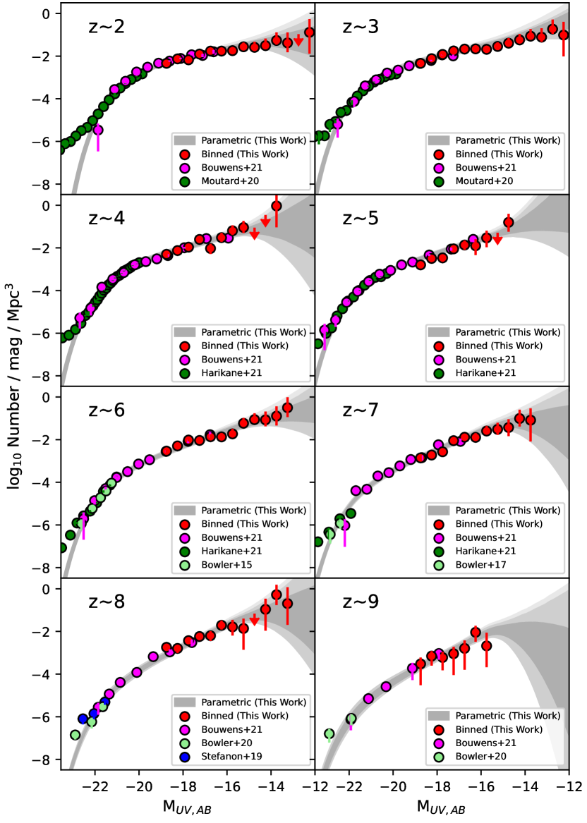
Figure 4.— The 68% and 95% likelihood contours (dark and light grey shaded regions, respectively) we derive on the shape of the $UV$ LFs at $z\sim 2$, $z\sim 3$, $z\sim 4$, $z\sim 5$, $z\sim 6$, $z\sim 7$, $z\sim 8$, and $z\sim 9$ based on our lensed HFF samples and the presented blank-field constraints on the LF. The presented contours give equal weight to the contours we derive treating the CATS, Sharon/Johnson, GLAFIC, and Keeton models as the truth in our forward-modeling procedure (Bouwens et al. 2017b) and then recover LF results using the median magnification factors from the other parametric lensing models. The red solid circles show the binned constraints (with $1\sigma$ error bars) we obtain by dividing the number of sources in a luminosity bin $N_{m}$ by the selection volume $V_{m}$ in that bin (Table 4). The red upper limits are $1\sigma$. The light red shaded region ($2\sigma$) indicates the LF constraints if we adopt larger sizes in modeling the completeness of the faintest sources, as per the Shibuya et al. (2015) size-luminosity relations. At $z\sim 2$-9, the blank-field constraints are from Bouwens et al. (2021a), but with comparisons to the results from Bouwens et al. (2007), Bouwens et al. (2015), Bowler et al. (2015), Bowler et al. (2017), Bouwens et al. (2019), Stefanon et al. (2019), and Bowler et al. (2020) also shown.

The observed agreement between the two results is remarkable given the enormous differences between the two approaches and their different challenges. For example, while blank-field probes provide us with less leverage in luminosity to constrain the faint-end slope $\alpha$ of the $UV$ LF, they are much less sensitive to assumptions about source size near the detection limits (since almost all sources at these limits are unresolved) and sample sufficient volume to obtain much better constraints on the bright end of the LF. Meanwhile, for lensing cluster probes, despite the sensitivity of this approach to an accurate modeling of the sizes (e.g., Bouwens et al. 2017a), the additional leverage provided by lensing allows us to probe substantially fainter in luminosity, providing us with much greater leverage to probe the faint-end slope. Figure 2 illustrates this leverage quite well.

We emphasize that our use of very small sizes is critical for achieving consistent faint-end slope $\alpha$ results to blank-field studies. As demonstrated in both Bouwens et al. (2017a) and Bouwens et al. (2022a), if we had instead assumed that galaxies followed a more standard size-luminosity relation (e.g., Huang et al. 2013; Shibuya et al. 2015), completeness would be a decreasing function of the magnification of the source. This would result in much steeper faint-end slopes $\alpha$ and significantly higher volume densities of sources $>$$-$15 mag (Bouwens et al. 2017a, 2022a).

This is the first time such consistent faint-end slope results have been found between blank-field and lensing-cluster analyses over such an extended range in redshift. The independence of the two approaches and their consistency strongly suggests that we can combine the two approaches to arrive at even more robust determinations of the overall shape and evolution of the $UV$ LF.

3.3.2 Leveraging Both Blank-Field and HFF Results

Having demonstrated we can use lensed samples of $z=2$-9 galaxies to obtain constraints on the faint-end slope $\alpha$ consistent with blank-field studies, we now leverage both data sets to arrive at our best overall estimate on the shape of the $UV$ LFs at $z=2$-9.

For our blank-field constraints on the $z\sim 2$-9 LF results, we rely on the likelihood constraints Bouwens et al. (2021a) derived from the comprehensive set of HST fields. Following the treatment we provided in Bouwens et al. (2017b), we again allow for a 20% uncertainty in the relative normalization of the value of blank-field and cluster LF results at $z\sim 2$, 3, 6, 7, 8, and 9. This 20% uncertainty includes a $\sim$15% contribution from cosmic variance (Robertson et al. 2014) and a $\sim$10% uncertainty in the selection volume calculation for both the bright and faint-end of the LFs. For our $z\sim 4$ and $z\sim 5$ results, we allow for a 26% and 18% cosmic variance uncertainty (and 28% and 22% relative uncertainty in total) owing to our consideration of lensed sources behind only 2 and 4 clusters, respectively, due to the challenge in identifying $z\sim 4$-5 galaxies behind those clusters without substantial contamination.

Additionally and motivated by the modest uncertainties in the size distribution of the faintest sources, we allow for modest uncertainties in the selection efficiency of galaxies in the faintest magnitude intervals. In particular, we consider both the impact of increasing the selection efficiencies in the 27.5-28.0 mag, 28.0-28.5 mag, 28.5-29.0 mag, and $>$29.0 mag intervals by 2%, 5%, 20%, and 30% and decreasing the selection efficiencies by the same amount and then marginalize the results over both the regularly calculated efficiencies and the two others. These percentage changes indicate the approximate impact of $\sim$10% differences between the model and derived S/N for sources of a given magnitude. For our derived LF parameters at $z\sim 2$ and 3, similar adjustments were made to selection volumes to determine the impact of possible systematics in the estimated volumes, but 1.2 and 0.7 mag brighter (corresponding to the shallower $UV_{275}$ and $U_{336}$ coverage over the HFF clusters and also shallower $z\sim 2$ and $z\sim 3$ selections).

In Figure 4, we show the 68% and 95% confidence intervals on our LF results marginalizing over the results for the four families of parametric models, i.e., GLAFIC, CATS, Sharon/Johnson, and Keeton, while comparing against independent constraints on the bright-end of the $UV$ LFs from various blank-field probes (Bouwens et al. 2007, 2015a, 2019, 2021a; Bowler et al. 2015, 2017, 2020; Stefanon et al. 2019; Harikane et al. 2021). Along with the formal confidence intervals, we also show the allowed LF results (light shaded region) if the mean sizes of lower luminosity galaxies are more consistent with the Shibuya et al. (2015) scalings. We stress that the observational results of Bouwens et al. (2017a), Kawamata et al. (2018), Bouwens et al. (2022a), and Yang et al. (2022) strongly suggest the true size distribution is significantly smaller than this, but show these allowed regions to present the possible systematic error.

For convenience, in Table 3, we include a compilation of our derived 68% confidence intervals for our $z=2$-9 LF results from $z\sim 9$ to $z\sim 2$. The formal uncertainties provided in Table 3 include not only the formal 68% confidence results from our MCMC fitting results using the parametric models, but include systematic uncertainties on the volume densities if the true sizes of lower luminosity galaxies are much larger than implied by the Bouwens et al. (2017a, 2017c), Kawamata et al. (2018), and Bouwens et al. (2022a) results.

We also include a simple binned version of our LF results in Figure 4 using the relation

$$\phi_{m}=\frac{N_{m}}{V_{m}}$$ (6)

where $\phi_{m}$ is the derived volume density of sources in magnitude bin $m$, $N_{m}$ is the number of sources in magnitude bin $m$, and $V_{m}$ is the estimated selection volume in magnitude bin $m$. We calculate $V_{m}$ as follows:

$$V_{m}=\int_{A}\int_{dz}C(z,m,\mu)\frac{1}{\mu(A)}\frac{d^{2}V(z)}{dzdA}dzdA$$ (7)

where $dA$ is a differential area in the image plane, $C(z,m,\mu)$ is the selection completeness as a function of redshift $z$, apparent magnitude $m$, an the magnification factor $\mu$, and $\frac{d^{2}V(z)}{dzdA}$ is a differential volume element. The plotted uncertainties in Figure 4 include not only the formal Poissonian uncertainties but also the systematic uncertainties on the volume densities if the true sizes of lower luminosity galaxies are as given by Bouwens et al. (2022a) size-luminosity relation instead of adopting point-source sizes. No account is made for the impact of uncertainties in magnification factors on the binned constraints. For convenience, we list the binned constraints shown in Figure 4 in Table 4.

Results derived using the individual parametric and non-parametric magnification models are presented in Table 7 of Appendix A. Figures 14 and 15 from Appendix A show the 68% and 95% confidence intervals on the $z\sim 2$ and $z\sim 6$ LF results, respectively, using the same set of parametric and non-parametric models. In general, very similar LF results are obtained utilizing different lensing models, with derived parameters typically differing by much less than the formal uncertainties derived for a single model. In general, LFs derived using the non-parametric lensing models showed higher values for the curvature parameter $\delta$. This appears to derive from the larger differences seen between the magnification factors from these models and those in the parametric lensing models and the impact this has in washing out potential turn-overs at the faint-end of the $UV$ LFs.

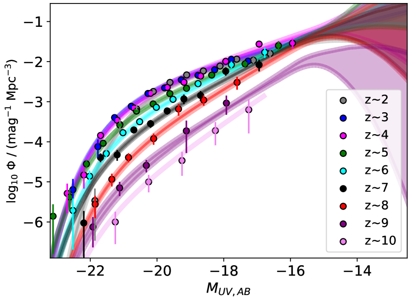
Figure 5.— The 68% likelihood contours we derive on the shape of the faint end of the $UV$ LFs at $z\sim 2$, $z\sim 3$, $z\sim 4$, $z\sim 5$, $z\sim 6$, $z\sim 7$, $z\sim 8$, and $z\sim 9$ based on our lensed HFF samples and the presented constraints on the LF from blank-field studies. The solid circles show our LF constraints from the Bouwens et al. (2021a) blank-field analysis. The $z\sim 10$ LF results shown here are from Oesch et al. (2018a) and rely on both blank-field and lensing-field results.

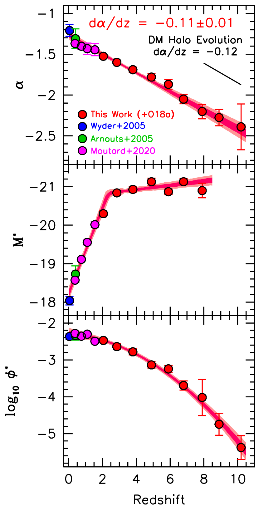
Figure 6.— Apparent evolution of the faint-end slope $\alpha$ (upper panel), characteristic luminosities $M^{*}$ (center panel), and normalization $\phi^{*}$ (lower panel) of the $UV$ LF with redshift. The red circles present the current LF constraints at $z=2$-9 and those of Oesch et al. (2018a) at $z\sim 10$, while the blue, green, and magenta circles give the Wyder et al. (2005), Arnouts et al. (2005), and Moutard et al. (2020) constraints at $z\sim 0.05$, $z\sim 0.4$, and over the redshift range $z\sim 0.3$-1.5. The shaded red line illustrates our best-fit relation for the evolution (§3.4). The evolution of the faint-end slope $\alpha$ is now extremely well determined as a function of redshift and remarkably consistent with the evolution expected based on the change in slope of the halo mass function (Tacchella et al. 2013, 2018; Bouwens et al. 2015a, 2021a; Mason et al. 2015; Mashian et al. 2016; Park et al. 2019). Previous work by Bouwens et al. (2015), Parsa et al. (2016), and Finkelstein (2016) arrived at very similar d$\alpha$/dz trends as what is found here by fitting to the available $\alpha$ determinations.

A summary of the mean LF parameters $M^{*}$, $\phi^{*}$, $\alpha$, and $\delta$ we derive on the basis of the four parametric magnification models (GLAFIC, CATS, Sharon/Johnson, Keeton) and the two non-parametric models (grale and Diego) is provided in Table 2 and are indicated by the descriptors “Parametric” and “Non-parametric,” respectively. Finally, figure 5 shows our best-fit $z\sim 2$, $z\sim 3$, $z\sim 4$, $z\sim 5$, $z\sim 6$, $z\sim 7$, $z\sim 8$, and $z\sim 9$ LFs, along with the $z\sim 10$ results from Oesch et al. (2018a). The $z\sim 10$ LF results from Oesch et al. (2018a) rely on both blank-field and lensing-field results. From the plotted constraints, it is clear that the $UV$-bright galaxies undergo a much more rapid evolution in volume density than galaxies at the faint end of the LF. In the next section, we parameterize the evolution of the $UV$ LF in terms of convenient fitting formulas.

3.4. Evolution of the Schechter Parameters with Cosmic Time

The availability of deep lensed sample of $z=2$-9 galaxies behind the HFF clusters have made it possible to significantly improve our constraints on the faint-end slope of the $UV$ LF and therefore the evolution of the $UV$ LF from $z\sim 10$ to $z\sim 2$.

Our estimates of the Schechter parameters in Table 2 provide a good illustration of this. Comparing the uncertainties on the faint-end slope $\alpha$ from our most recent blank-field determinations, i.e., Bouwens et al. (2021a), and those combining blank-field constraints with the lensing cluster constraints, we have been able to reduce the uncertainties on the faint-end slope $\alpha$ by a factor of $\sim$1.5, 2, 2, 2, and 2 at $z\sim 5$, 6, 7, 8, and 9, respectively.

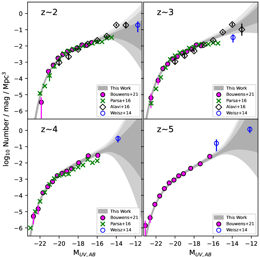
Figure 7.— Comparison of the new $z=2$-5 $UV$ LFs we have derived from the HFFs (light and dark grey shaded regions) and the new blank-field results of Bouwens et al. (2021a: solid magenta circles) against previous LF results in the literature including those from Parsa et al. (2016: green crosses), Alavi et al. (2016: black open diamonds), and Weisz et al. (2014: open blue circles). While the comparisons here focus on previous results focusing on the faint-end of the $UV$ LF, comparisons to brighter $UV$ LF work (e.g., Steidel et al. 1999; Reddy & Steidel 2009; Oesch et al. 2010; van der Burg et al. 2010; Finkelstein et al. 2015; McLeod et al. 2016; Mehta et al. 2017; Adams et al. 2020) can be found in Bouwens et al. (2021a). See §4.1 for discussion.

Taking advantage of these new constraints, we are in position to further refine our characterization of the evolution in each Schechter parameters. Following Bouwens et al. (2021a), we fit the evolution in $\alpha$ as a linear function of redshift, $\log_{10}$ $\phi^{*}$ as a quadratic function of redshift, and $M^{*}$ as a linear function of redshift, with a break at $z\sim 2.5$. Simultaneously fitting the present LF constraints over the redshift range $z\sim 2$-9 as well as the Oesch et al. (2018a) results at $z\sim 10$, we find the following best-fit relation:

$$M_{UV}^{*}= \left\{\begin{array}[]{ll}(-20.87\pm 0.08)+(-1.10\pm 0.06)(z-z_{t}),&\textrm{for}~{}z<z_{t}\\ (-21.04\pm 0.04)+(-0.05\pm 0.02)(z-6),&\textrm{for}~{}z>z_{t}\\ \end{array}\right.$$

$$\phi^{*}= (0.38\pm 0.03)(10^{-3}\textrm{Mpc}^{-3})10^{(-0.35\pm 0.01)(z-6)+(-0.027\pm 0.004)(z-6)^{2}}$$

$$\alpha= (-1.95\pm 0.02)+(-0.11\pm 0.01)(z-6)$$

where $z_{t}=2.42\pm 0.09$. Figure 6 compares the observed evolution of $\alpha$, $M^{*}$, and $\phi^{*}$ with the above relation.

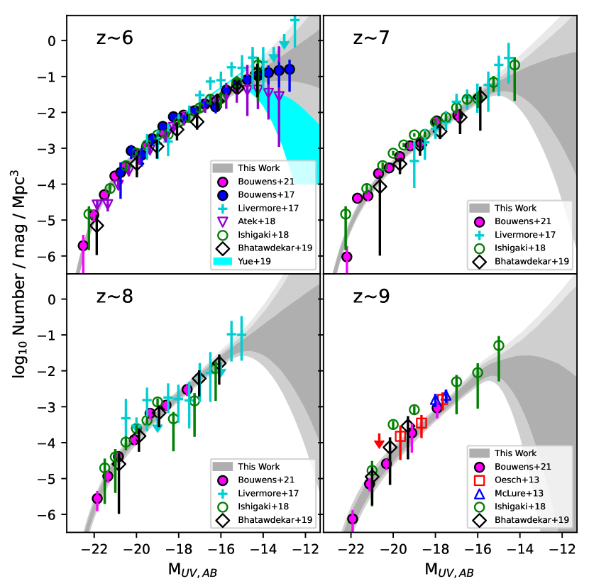
Figure 8.— Similar to Figure 7 but for our derived LFs at $z=6$-9. Included in these comparisons are the blank-field results of Bouwens et al. (2021a: solid magenta circles), McLure et al. (2013: open blue triangles), and Oesch et al. (2013: open red squares) and the HFF results of Livermore et al. (2017: bluish green plus signs), Bouwens et al. (2017b: solid blue circles), Ishigaki et al. (2018: open green circles), Atek et al. (2018: open purple triangles), Yue et al. (2018: shaded cyan region), and Bhatawdekar et al. (2019: open black diamonds). See §4.1.

As we previously noted (Bouwens et al. 2015a, 2021a), the evolution in the faint-end slope $\alpha$ agrees remarkably well with change in slope expected based on the evolution of the halo mass function over the same range in redshift, i.e., $d\alpha/dz\sim-0.12$ (Bouwens et al. 2015a). This is fairly similar to the faint-end slope evolution we recovered in Bouwens et al. (2015a), i.e., $d\alpha/dz\sim-0.10\pm 0.03$, the $d\alpha/dz\sim-0.11\pm 0.01$ trends derived by Parsa et al. (2016) and Finkelstein (2016) fitting to the available $z\sim 0$-10 and $z\sim 4$-10 LF results, respectively, and $d\alpha/dz\sim-0.09\pm 0.05$ trend recently derived by Bowler et al. (2020: but who express the LF evolution they derive using a double power-law form).

The slow evolution in the characteristic luminosity $M^{*}$ at $z>z_{t}$ seems very likely to be a consequence of the fact that $UV$ luminosity reaches a maximum value of $\sim-21$ to $-23$ mag due to the increasing importance of dust extinction in the highest stellar mass and SFR sources (Bouwens et al. 2009a; Reddy et al. 2010). Finally, as Bouwens et al. (2015a, 2021a) have argued, the evolution in $\phi^{*}$ can readily be explained by evolution in the halo mass function and no significant evolution in the star formation efficiency. As in Bouwens et al. (2021a), we find that $\log_{10}$ $\phi^{*}$ depends on redshift with a clear quadratic dependence (but here significant at $6\sigma$ instead of $4\sigma$).

4. Discussion

4.1. Comparison with Previous LF Results

Before discussing in more detail the implications of the present LF determinations, it makes sense to compare our new results with the many previous determinations of these LFs that exist in the literature. Comparing with previous work is very valuable for improving LF determinations in general, as it allows us to identify differences in the results and ascertain the best path to improve LF results in the future.

To this end, we present our new $z\sim 2$, 3, 4, 5, 6, 7, 8, and 9 LF results in Figures 7 and 8 using the 68% and 95% confidence intervals we have derived (light grey and dark grey shaded regions, respectively). For the comparisons we provide, we will focus on previous LF results that provided results on the faint-end of the $z=2$-9 LFs. In the preparatory work to this using blank-field data (Bouwens et al. 2021a), we already provided a significant discussion of previous LF results which are more relevant for the bright end of the $UV$ LFs (their §4.1).

To help with the discussion of various faint-end LF results, we also include on Figure 7 and 8 the approximate regions in parameter space allowed if we take galaxy sizes to follow the Bouwens et al. (2022a) size-luminosity relation (light shaded regions above the nominal 68% and 95% contours).

Table 568% and 95% Confidence Intervals on the $UV$ Luminosity Density at $z\sim 2$-9 to Various Limiting Luminosities

	$\log_{10}\rho_{UV}$ ($UV$ Luminosity Density)
	(ergs s-1 Hz-1 Mpc-3)
	Lower Bound		Upper Bound
Faint-End Limit	95%	68%	68%	95%
	$z\sim 2$
$M_{UV}<-17$	26.38	26.41	26.46	26.49
$M_{UV}<-15$	26.46	26.49	26.54	26.57
$M_{UV}<-13$	26.48	26.51	26.57	26.60
$M_{UV}<-10$	26.48	26.51	26.59	26.68
	$z\sim 3$
$M_{UV}<-17$	26.45	26.51	26.64	26.70
$M_{UV}<-15$	26.52	26.58	26.72	26.77
$M_{UV}<-13$	26.56	26.62	26.76	26.81
$M_{UV}<-10$	26.58	26.66	26.88	26.94
	$z\sim 4$
$M_{UV}<-17$	26.42	26.47	26.56	26.60
$M_{UV}<-15$	26.52	26.56	26.66	26.70
$M_{UV}<-13$	26.56	26.62	26.82	27.01
$M_{UV}<-10$	26.58	26.71	29.18	31.17
	$z\sim 5$
$M_{UV}<-17$	26.24	26.27	26.35	26.38
$M_{UV}<-15$	26.35	26.38	26.46	26.50
$M_{UV}<-13$	26.39	26.44	26.62	26.87
$M_{UV}<-10$	26.39	26.45	28.52	30.84
	$z\sim 6$
$M_{UV}<-17$	26.08	26.12	26.20	26.24
$M_{UV}<-15$	26.23	26.26	26.34	26.38
$M_{UV}<-13$	26.28	26.32	26.43	26.50
$M_{UV}<-10$	26.29	26.34	26.58	27.04
	$z\sim 7$
$M_{UV}<-17$	25.92	25.95	26.01	26.05
$M_{UV}<-15$	26.11	26.14	26.23	26.27
$M_{UV}<-13$	26.15	26.20	26.33	26.41
$M_{UV}<-10$	26.15	26.20	26.41	26.68
	$z\sim 8$
$M_{UV}<-17$	25.55	25.61	25.72	25.78
$M_{UV}<-15$	25.85	25.89	26.01	26.07
$M_{UV}<-13$	25.90	25.96	26.20	26.41
$M_{UV}<-10$	25.90	25.96	26.43	28.01
	$z\sim 9$
$M_{UV}<-17$	24.99	25.07	25.26	25.34
$M_{UV}<-15$	25.33	25.39	25.54	25.60
$M_{UV}<-13$	25.36	25.43	25.65	25.75
$M_{UV}<-10$	25.36	25.43	25.67	25.82

We will structure the comparisons we make to previous work as an increasing function of redshift:

$\mathbf{z\sim 2}$-5: To the present, there have been only two studies which have reported LF results on the extreme faint end of the $UV$ LF at $z\sim 2$-5, i.e., at $>-16$ mag, for Lyman-break galaxies, one by Alavi et al. (2016) based on lensed samples of $z\sim 1$-3 galaxies identified behind two HFF clusters Abell 2744 and MACS0717 and Abell 1689 and a second by Parsa et al. (2016) using a deep ($\sim$30.5 mag) photometric redshift selection over the HUDF. The faint constraints reported by Alavi et al. (2016) and Parsa et al. (2016) lie above and below our own constraints and reach very different conclusions. Alavi et al. (2016) report a faint-end slope from their LF results of $-1.72\pm 0.04$ and $-1.94\pm 0.06$ at $z\sim 2$ and $z\sim 3$, respectively, while Parsa find $-1.31\pm 0.04$ and $-1.31\pm 0.04$ at approximately same redshifts.

As illustrated in Figure 2, the leverage available from our lensed HFF samples should allow us to quantify the faint-end slope for the $UV$ LF $z\sim 2$ and $z\sim 3$ with great precision, if an accurate account can be made for various sources of systematic errors. Given the consistency of our own blank-field and lensed measurements of the faint end of the $z\sim 2$ and $z\sim 3$ LF, what might drive the lower and higher volume density results obtained by Parsa et al. (2016) and Alavi et al. (2016)? For the faint end of the Parsa et al. (2016) probe, the answer is not entirely clear, as their LF determinations are in good agreement with both the Bouwens et al. (2021a) blank-field LF results and our lensed results brightward of $-16.5$ mag and appear to drive the differences in our faint-end slope inferences. Faintward of $-16.5$ mag, differences between the Parsa et al. (2016) LF measurements and our own are more significant. One potential concern for the LF determinations of Parsa et al. (2016) is the inclusion of sources to $\sim$30.5-31.0 mag, i.e., at essentially the detection limit of the HUDF. At such faint magnitudes, segregating sources into different redshift bins is more challenging, especially given that the $UV$ observations Parsa et al. (2016) report utilizing (essential for probing the position of the Lyman break) have a $5\sigma$ depth of 28 mag, i.e., $\sim$10$\times$ brighter than the $z\sim 1$-4 sources being included in their LFs.

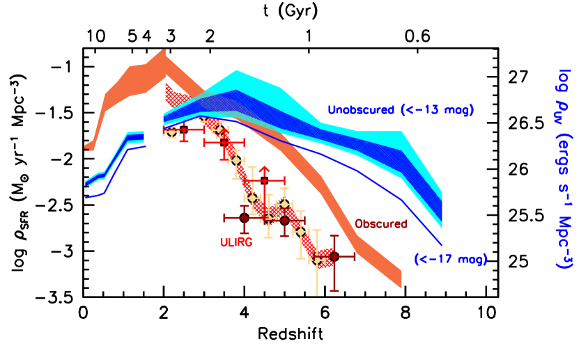
Figure 9.— 68% and 95% confidence intervals on the inferred $UV$ luminosity density and unobscured star formation rate density (blue and cyan shaded regions) at $z\sim 2$-9 derived from our new $UV$ LF results integrated down to $-$13 mag (§4.2). Also shown are the obscured SFR density results (orange-shaded region) derived by Bouwens et al. (2020) from $z\sim 8$ to $z\sim 2$ by applying the ASPECS IRX results to $z\sim 4$-8 samples, making use of published ULIRG results (shown with the hatched red region) by Wang et al. (2019: dark red points), Franco et al. (2020: red points), and Dudzevičiūtė et al. (2020: solid brownish-yellow circles), and adopting the $z=2$-3 dust extinction estimates from Reddy & Steidel (2009). The shaded orange region from $z=0$ to $z=2$ shows the constraints on the obscured SFR density from Magnelli et al. (2013), while the blue and cyan shaded regions at $z<2$ show the constraints from Wyder et al. (2005) and Moutard et al. (2020). The blue lines show the $UV$ luminosity densities and SFR densities we derive from our LF results brightward of $-$17 mag at $z>2$ and Wyder et al. (2005) and Moutard et al. (2020) find at $z<2$. As Bouwens et al. (2009a, 2016b), Dunlop et al. (2017), and Zavala et al. (2021) have previously concluded, the bulk of the SFR density is unobscured at $z>4$ and obscured at $z<4$. There is a transition between the two regimes at $z=4$.

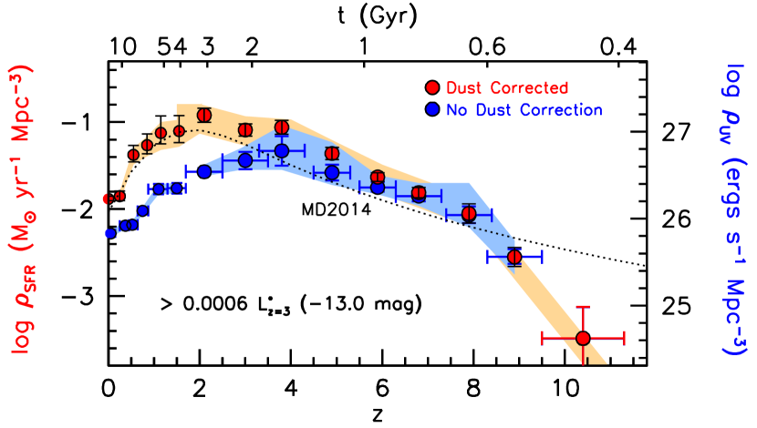
Figure 10.— Unobscured and dust-corrected SFR density of the universe (blue and red solid circles, respectively, with $1\sigma$ error bars) derived from our new $UV$ LF results at $z=2$-9 and integrating down to $-13$ mag (as in Figure 9). The right axis gives the equivalent $UV$ luminosity density vs. redshift. The light blue shaded contours indicate approximate 95% confidence intervals on the unobscured SFR and $UV$ luminosity densities, while the light red shaded contours illustrate the overall trends in the evolution of the SFR density. The present determinations of the SFR density is higher than similar determinations Madau & Dickinson (2014: dotted line) due to our integrating $\sim$4 mag further down the $UV$ LF (to a faint-end limit of $-13$ mag vs. $-17$ mag used by Madau & Dickinson 2014), use of new constraints on the obscured SFR density at $z\geq 4$ from ALMA and Herschel (shown in Figure 9), and use of the Magnelli et al. (2013) constraints at $z\leq 2$.

Alavi et al. (2016)’s $z\sim 2$-3 LF results are higher than our own for the faintest sources ($>$$-$15 mag). This almost certainly results from the completeness corrections Alavi et al. (2016) calculate extrapolating the Shibuya et al. (2015) size-luminosity relation to lower luminosities, and in fact making use of a similar size luminosity relation we find a $3\times$ higher volume density for the faintest sources, largely reproducing Alavi et al. (2016)’s results. It is worth emphasizing that use of the size-luminosity relation from Shibuya et al. (2015) for completeness calculations was very reasonable, given the lack of information that existed five years ago regarding the sizes of the faintest sources at $z\sim 2$-3.

Finally, we include some constraints on the $z\sim 2$-5 LFs of galaxies by Weisz et al. (2014) that rely on resolved stellar population analyses of nearby dwarf galaxies, abundance matching, and evolving the luminosities of these dwarf galaxies backwards in time (see also Boylan-Kolchin et al. 2015). While such analyses are obviously very interesting to pursue and should be useful in providing indicative constraints on the volume density of faint sources during the first few billion years of the universe, they also necessarily involve a number of significant assumptions regarding the precise history of the stars that make up these analyses (e.g., mergers, galaxy disruption, etc.). Given the uncertainties, it is encouraging how consistent the Weisz et al. (2014) LF inferences and our own results are.

$\mathbf{z\sim 6}$-9: At lower luminosities, our new $z\sim 6$-7 LF results from the HFFs are in excellent agreement with the $z\sim 6$-7 results from Atek et al. (2015b) using the first three HFF clusters, the $z\sim 5$-10 results from Castellano et al. (2016) based on the first two HFF clusters, our previous results obtained from the first four HFF clusters (Bouwens et al. 2017b), the $z\sim 6$-7 results from Atek et al. (2018) based on the full HFF program, the Yue et al. (2018) results based on the first four HFF clusters, and the LF results obtained by both McLure et al. (2013) and Oesch et al. (2013) at $z\sim 9$. The $z=6$-9 LF results of Bhatawdekar et al. (2019) also appear to be in reasonable agreement with our own LF results, particularly if the comparison is made against their results modeling the sizes of faint galaxies as “disk galaxies” (with a mean size of 0.15^′′). Given the very small sizes adopted in our analysis, we would have expected the “point-source” results from Bhatawdekar et al. (2019) to be most consistent with our own, but the point-source results from Bhatawdekar et al. (2019) are $\sim$1.5$\times$ lower; it is not clear why this would be the case.

Table 6$UV$ Luminosity Densities and Star Formation Rate Densities to $-13.0$ AB mag (0.0006 $L_{z=3}^{*}$: §4.2)

Lyman		$\textrm{log}_{10}\mathcal{L}$	$\textrm{log}_{10}$ SFR density
Break		(ergs s-1	($M_{\odot}$ Mpc-3 yr-1)
Sample	$<z>$	Hz-1 Mpc-3)	Unobscured	Obscured	Total
U275	2.1	26.54$\pm$0.03	$-$1.61$\pm$0.03	$-$1.07$\pm$0.10	$-$0.96$\pm$0.08
U336	3.0	26.69$\pm$0.07	$-$1.46$\pm$0.07	$-$1.36$\pm$0.10	$-$1.11$\pm$0.07
B	3.8	26.74$\pm$0.12	$-$1.41$\pm$0.12	$-$1.47$\pm$0.10	$-$1.14$\pm$0.08
V	4.9	26.54$\pm$0.09	$-$1.62$\pm$0.09	$-$1.81$\pm$0.10	$-$1.40$\pm$0.07
i	5.9	26.38$\pm$0.05	$-$1.78$\pm$0.05	$-$2.28$\pm$0.10	$-$1.66$\pm$0.05
z	6.8	26.27$\pm$0.06	$-$1.89$\pm$0.06	$-$2.93$\pm$0.10	$-$1.85$\pm$0.06
Y	7.9	26.08$\pm$0.12	$-$2.07$\pm$0.12	$-$3.31$\pm$0.10	$-$2.05$\pm$0.11
J	8.9	25.54$\pm$0.11	$-$2.61$\pm$0.11	—	$-$2.61$\pm$0.11

Our LF results at $z=6$-8 also show good overall agreement with the results from Livermore et al. (2017) brightward of $-17$ mag. At lower luminosities, the differences are larger. We refer interested readers to §6.2 of Bouwens et al. (2017a) and §6.2-6.3 of Bouwens et al. (2017b) for a discussion of the differences. Our results also show a broad similarity to the $z\sim 6$-9 LF results of Ishigaki et al. (2018), but we note a slight excess in the volume density of sources they find in their $z\sim 6$-7 LF results and $z\sim 9$ results (upper and lower right panels of Figure 8) at $\sim-19$ mag and a slight deficit in their $z\sim 8$ LF results at $\sim-18$ to $-17$ mag. The slightly higher volume densities that Ishigaki et al. (2018) find in their LF results at $z\sim 9$ may derive from their probing a slightly lower redshift range with their $z\sim 9$ selection than we do in our own determinations. Use of the photometric redshift estimates from Ishigaki et al. (2018: their Table 8) substantiates this assertion, as Ishigaki et al. (2018) probe a mean redshift of $z\sim 8.5$ with their $z\sim 9$ selection and we probe a mean redshift of $z\sim 8.9$. The slight deficit Ishigaki et al. (2018) report at $-18$ and $-17$ mag in their $z\sim 8$ LF results appears to derive from the limited number of sources Ishigaki et al. (2018) have in the faintest bins, i.e., 1, 1, and 3, respectively.

4.2. UV Luminosity and SFR Densities

Given the impressively deep $UV$ LF results we have over the redshift range $z=2$-9, it is clearly interesting to use these measurements to map out the evolution of the $UV$ luminosity density of galaxies to very faint luminosities from $z\sim 9$ to $z\sim 2$.

To maximize the utility of this exercise, we have elected to compute luminosity density to the faint-end limits $-17$ mag, $-15$ mag, $-13$ mag, and $-10$ mag. We adopted those faint-end limits due to their frequent use in both blank-field LF studies and reionization calculations (e.g., Robertson et al. 2013, 2015; Bouwens et al. 2015b; Ishigaki et al. 2018).

To compute the luminosity densities implied by our new LF results, we simply compute the luminosity density implied by various parameterizations and marginalize across the likelihood distribution. We compute both 68% and 95% confidence intervals on the luminosity densities and have tabulated our results in Table 5. The results are also presented in Figure 9. From the results presented in both the table and figures, it is clear that probes to $-13$ mag contribute meaningfully to the $UV$ luminosity density vis-a-vis probes to $-$17 mag, increasing the total $UV$ luminosity by 0.1 dex (st $z\sim 2$) and by 0.4 dex (at $z\sim 8$).

Remarkably, the present observational results allow us to constrain the luminosity densities to an uncertainty of $<$0.05 dex at $z\sim 2$-3 and $z\sim 6$-7 and $<$0.12 dex at $z\sim 4$-5 and $z\sim 8$-9, equivalent to a $<$13% and $<$30% relative uncertainty, respectively. The $UV$ luminosity densities we derive brightward of $-10$ mag are much less well constrained. While the 95% confidence intervals we derive from our $z\sim 2$-3, $z\sim 6$-7, and $z\sim 9$ results span a $\lesssim$0.5 dex range, these same intervals span $\gtrsim 2$ dex range at $z\sim 4$-5 and $z\sim 8$.

It is interesting to convert our new determinations of the $UV$ luminosity density into equivalent star formation rate densities using the conversion factors in Madau & Dickinson (2014). Assuming a Chabrier (2003) IMF, a constant star formation rate, and metallicity $Z=0.002$ $Z_{\odot}$, the conversion factor $\cal{K}$_FUV is $0.7\times 10^{-29}M_{\odot}\,\textrm{year}^{-1}\,\textrm{erg}^{-1}\,\textrm{s}\,\textrm{Hz}$. The specific value adopted for the metallicity does not have a huge impact on this conversion factor ($<$1.5%: Madau & Dickinson 2014). The equivalent SFR densities to the integrated $UV$ luminosity densities to $-$13 mag are also shown on the left vertical axis of Figure 9.

We have compared the implied unobscured SFR density from our $UV$ LF results in Figure 9 and have compared it to obscured SFR density inferred from the Bouwens et al. (2020) ASPECS HUDF study, the obscured SFR density results at $z=0$-2 from Magnelli et al. (2013) and the unobsucred SFR density results from $z=0$ to $z=1.5$ from Wyder et al. (2005) and Moutard et al. (2020). We also present the unobscured SFR density inferred at $z\geq 2$ integrated down to a brighter limit, $-17$ mag, similar to what Madau & Dickinson (2014) utilize in their SFR density figures.

For convenience, Table 6 presents our new SFR density estimates along with the estimates of the obscured SFR densities Bouwens et al. (2020) derived combining their own inferences of the obscured star formation from their ASPECS HUDF results with the ULIRG results of Wang et al. (2019), Franco et al. (2020a), and Dudzevičiūtė et al. (2020). We adopt a fiducial 0.1 dex uncertainty in the obscured SFR densities at $z\geq 2$ given the considerable challenges in deriving star formation rates from far-IR SEDs resulting from the uncertain SED shapes, uncertain contribution from AGN, and uncertainties in the selection volume. Figure 10 compares the unobscured SFR densities to the total SFR densities.

It is clear from these results that unobscured star formation dominates the SFR density in the high-redshift universe and obscured star formation dominates the SFR density at intermediate and low redshift. As has been found before (e.g., Bouwens et al. 2009a, 2016b; Dunlop et al. 2017; Zavala et al. 2021), we find that the cross-over point between these two regimes is at $z\sim 4$. Additionally, it is interesting to note the impact that the faint-end limit can have on the transition redshift between the two regimes. In the Bouwens et al. (2020) ASPECS study, the transition redshift was $z\sim 5$ using a brighter faint-end limit of $-$17 mag, but using a faint-end limit of $-$13 mag, enabled by our new HFF results, we find a transition redshift $z\sim 4$.

4.3. Faint End Form of the LF and Existence of A Possible Turn-over

Thanks to the faintness of lensed HFF samples, our new constraints put us in position to set constraints where the $UV$ LF might turn over at the faint end. This question is relevant both because it provides insight into the efficiency of star formation in lower-mass galaxies (Behroozi et al. 2013) and because it allows for a more accurate accounting for the contribution of ionizing photons from especially faint star-forming galaxies.

As in Bouwens et al. (2017b), we can constrain the brightest magnitude where a turn-over in the LF can possibly occur using Eq. 3 and the overall likelihood distribution we have derived on the three parameters $M^{*}$, $\alpha$, and $\delta$. By marginalizing over the results we have obtained on the $UV$ LF at $z=2$-9 based on the four different families of parameterized lensing models, we can derive 68% and 95% confidence intervals on the $UV$ luminosity of the turn over.

We present in the upper panel of Figure 11 the constraints we are able to obtain on the position of the turn-over in the $UV$ LF for star-forming galaxies from $z\sim 9$ to $z\sim 2$. We find that our results rule out the presence of a turn-over brightward of $-15.5$ mag (95% confidence) for all $z=2$-9 samples we consider. We are able to obtain our tightest constraints on the luminosity of a possible turn-over at $z\sim 3$, where our results rule out the presence of a turn-over brightward of $-13.1$ mag (95% confidence). We note that Alavi et al. 2014 had previously presented evidence for the $UV$ LF at $z\sim 2$ extending so faint. At $z\sim 6$, our results rule out the presence of a turn-over brightward of $-14.3$ mag.

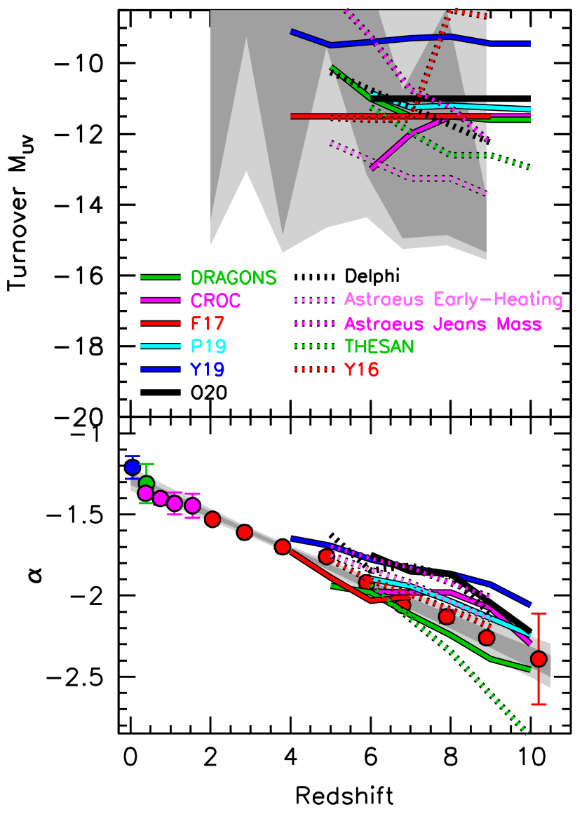
Figure 11.— (upper panel) 68% and 95% confidence intervals (dark and light grey shaded regions, respectively) on the $UV$ luminosity of the turn-over in the $UV$ LF obtained from our analysis (§3.3.2) of the lensed $z=2$-9 HFF samples (Bouwens et al. 2022b). The turn-over luminosities in the various theoretical LFs (§4.4) are also shown as a function of redshift. Our new LF results rule out the presence of a turn-over in the $UV$ LF brightward of $\approx-15.5$ mag (95% confidence) over the entire redshift range $z=2$-9. At $z\sim 3$, our LF results rule out the existence of such a turn-over brightward of $-13.1$ mag (95% confidence). (lower panel) Comparison of our derived redshift trend for the faint-end slope $\alpha$ (Figure 6: dark and light grey shaded regions indicate the 68% and 95% confidence regions, respectively) with that seen in the theory LFs (§4.4) as a function of redshift. Both the luminosity of the turn-overs $M_{T}$ and the faint-end slopes of the theory LFs appear to be in excellent overall agreement with our observational constraints.

Interestingly enough, our $z\sim 9$ LF results seem consistent with a turn-over at $-$15 mag. While indeed this would be interesting if this were the case, it is challenging to establish the robust presence of a turn-over in the LF at $z\sim 9$ due to the small number of sources expected faintward of $-16$ mag, and therefore our results cannot even establish the presence of a turn-over at $2\sigma$ significance. To make matters even more challenging, another complicated factor is the impact incompleteness in faint samples could have on the results. If faint sources have larger sizes than adopted here based on several recent observational probes (Bouwens et al. 2017a, 2022a; Kawamata et al. 2018; Yang et al. 2022), this would result in faint sources being much less complete in our selections than in our simulations and cause us to systematically underestimate the volume density of faint galaxies. This would cause the actual luminosity of a turn-over in the $UV$ LF to be substantially fainter than what we infer.

In general, the present constraints on the luminosity of a turn-over in the LF are consistent with most previous results in the literature. Atek et al. (2015b, 2018), Castellano et al. (2016), Livermore et al. (2017), Bouwens et al. (2017b), and Yue et al. (2018) all agree that the HFF results provide strong evidence against the $UV$ LF showing a turn-over brightward of $-$15 mag. At $z\geq 6$ and faintward of $-$15 mag, there has been a wide variety of differing conclusions drawn about whether firm constraints can be set regarding the existence of a turn-over and how faint those constraints extend (e.g., Castellano et al. 2016; Livermore et al. 2017; Bouwens et al. 2017b; Atek et al. 2018; Yue et al. 2018).

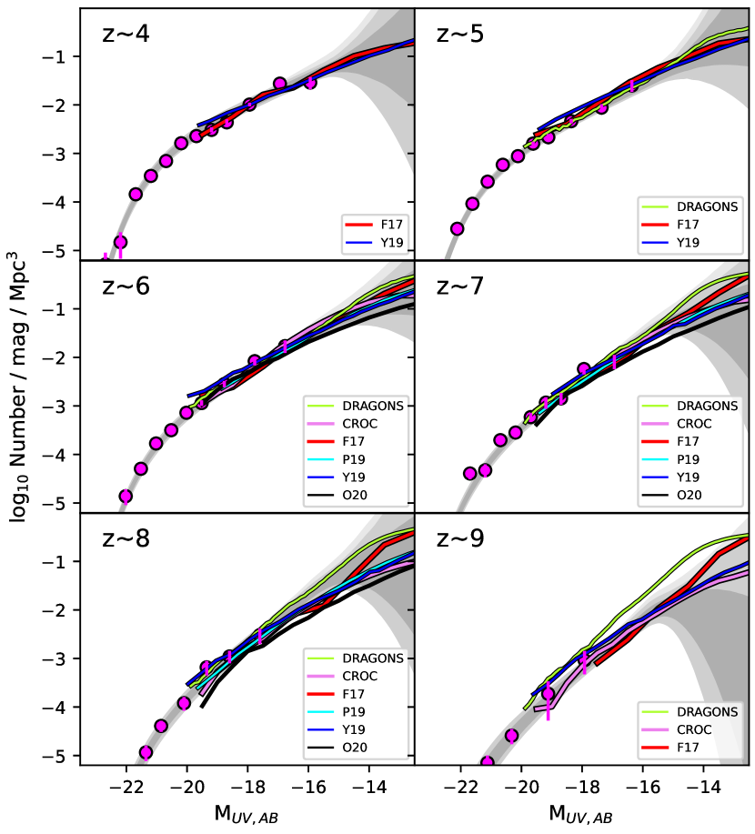
Figure 12.— Comparison of the 68% and 95% likelihood contours we derive for the $z=4$-9 LFs (dark and light grey shaded regions, respectively) with the predictions of the DRAGONS (Liu et al. 2016), CROC (Gnedin 2016), Finlator et al. (2017), Park et al. (2019), Yung et al. (2019), and Ocvirk et al. (2020). The solid magenta circles show the blank-field results obtained by Bouwens et al. (2021a). The LF results are only shown faintward of $-20$ mag to focus on the faint-end form of the models and not the behavior of the models at the bright end where treatment of dust extinction can play a dominant role. No comparison is made to $z\sim 2$-3 due to the general lack of model LF predictions for these redshift intervals. In general, we find excellent consistency between our new observational results and the different expectations from the theoretical models.

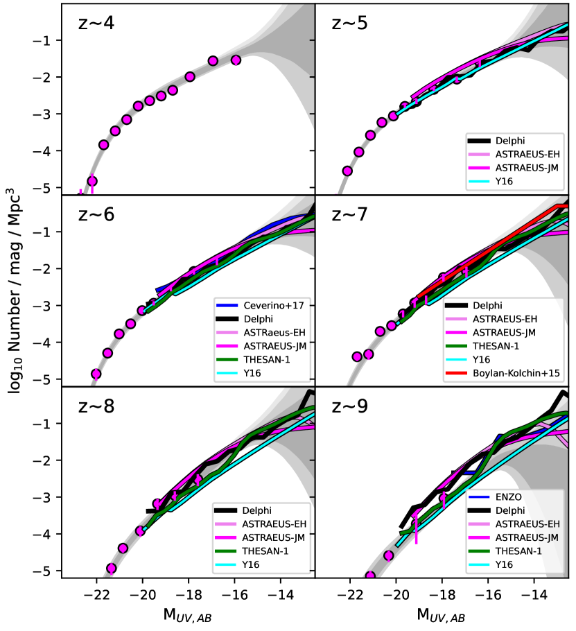
Figure 13.— Similar to Figure 12, but for the Delphi model (Dayal et al. 2014, 2022), FirstLight (Ceverino et al. 2017), ASTRAEUS-EarlyHeating (Hutter et al. 2021), ASTRAEUS-JeanMass (Hutter et al. 2021), ENZO (O’Shea et al. 2015), THESAN project (Kannan et al. 2022), and Yue et al. (2016: Y16). Also shown with the red line is the abundance matching constraints on the LF at $z\sim 7$ from the Boylan-Kolchin et al. (2015) analysis.

4.4. Comparison with Theoretical Models for the $UV$ LF

Finally, it is useful for us to compare the current constraints on the evolution of the $UV$ LF with that available from a number of recent theoretical models and cosmological hydrodynamical simulations. While we had previously looked at this in §6.3 of Bouwens et al. (2017b), here we have the advantage that we can compare the simulation/theory results with our new $UV$ LF results over a much more extended baseline in both redshift and cosmic time, reaching from $z\sim 9$ to $z\sim 4$. While no comparisons are made at $z\sim 2$ and $z\sim 3$ due to the lack of published model LF results in these two redshift intervals, it would be presumably possible to derive such LF results in the near future based on a number of on-going simulation efforts, e.g., the IllustrisTNG (Pillepich et al. 2018; Springel et al. 2018; Naiman et al. 2018; Nelson et al. 2018) and NewHorizons (Dubois et al. 2021) simulations.

We consider the following theoretical models:

DRAGONS [Liu et al. 2016]: The LF results from Liu et al. (2016) rely on the Dark-ages Reionization And Galaxy-formation Observables from Numerical Simulations (DRAGONS) project which build semi-numerical models of galaxy formation on top of halo trees derived from N-body simulations done over different box sizes to probe a large dynamical range. The semi-numerical models include gas cooling physics, star formation prescriptions, feedback and merging prescriptions, among other components of the model. The turn-over in the LF results of Liu et al. (2016) at $\sim-11.5$ mag correspond to the approximate halo masses $\sim 10^{8}$ $M_{\odot}$ where the gas temperature is $10^{4}$ K. Above this temperature, atomic cooling processes become efficient.

CROC [Gnedin 2014, 2016]: The model LF results for the Cosmic Reionization On Computers (CROC) were computed using gravity + hydrodynamical simulations executed with the Adaptive Refinement Treement (ART) code (Kravtsov 1999; Kravtsov 2002; Rudd et al. 2008). A wide variety of physical processes, including gas cooling and heating, molecular hydrogen chemistry, star formation, stellar feedback, radiative transfer of ionizing and UV light from stars is included in these simulations and done 20h^-1 Mpc boxes at a variety of resolutions. There is a flattening in the effective slope of CROC LFs to fainter magnitudes, with a peak at $\sim-12$ mag. However, the peak at $\sim-11.5$ mag is reported to depend on the minimum particle size in the simulations and thus not to be a robust result of the simulation.

Finlator et al. 2015, 2016, 2017 [F17]: The Finlator et al. (2015, 2016, 2017) LF results are derived from a cosmological simulation of galaxy formation in a $(7.5h^{-1})^{3}$ Mpc³ volume of the universe including both gravity and hydrodynamics. It is implemented in the GADGET-3 code (Springel 2005). Gas cooling has been added to this code through collisional excitation of hydrogen and helium (Katz et al. 1996). Metal line cooling is implemented using the collisional ionization equilibrium tables from Sutherland & Dopita (1993). Star formation is included using the Kennicutt-Schmidt law, with supernovae feedback implemented following the ”ezw” prescription from Davé et al. (2013) and metal enrichment from supernovae as in Oppenheimer & Davé (2008). Less efficient gas cooling at lower halo masses results in a flattening of the Finlator et al. (2015, 2016, 2017) LF results at the faint end, with the turn-over in the LF occuring at $\sim$$-$11.5 mag.

Park et al. 2019 [P19]: The Park et al. (2019) LF results are based on a flexible, physically motivated modeling of star formation in galaxy halos. In their model, Park et al. (2019) take the star formation efficiency (SFE), the SFE scaling with halo mass, and a turn-over mass to be free parameters which they then fit to the LF constraints from Bouwens et al. (2015a), Bouwens et al. (2017b), and Oesch et al. (2018a). In their fits, Park et al. (2019) allow for the turn-over mass to be between $10^{8}$ $M_{\odot}$ and $10^{10}$ $M_{\odot}$. Given that the tuning of the Park et al. (2019) LF model to match the observations of Bouwens et al. (2015a) and Bouwens et al. (2017b), it is not especially surprising that their model fits our new observational constraints quite well. The approximate turn-over luminosity in the Park et al. (2019) results occurs at $\sim$$-$11.3 mag.

Yung et al. 2019 [Y19]: The Yung et al. (2019) LF results are based on a recent version of the Santa Cruz semi-analytic model (Somerville et al. 2015), which includes not only merger trees constructed by a standard Press-Schechter formalism (Lacey & Cole 1993), but also gas cooling, star formation, chemical evolution, and SNe-driven winds, photoionization feedback, and a critical molecular hydrogen surface density necessary for star formation. Yung et al. (2019) produced their results to provide semi-analytical model forecasts for JWST and rely on halos with circular velocities $V_{\text{vir}}\approx 20-500$ km/s. Yung et al. (2019) report that SNe feedback play the dominant role in flattening the LF at the faint end. The turn-over at $M_{UV,AB}\sim-9$ mag is imposed as a result of the atomic cooling limit in halos with $V_{\text{vir}}\approx 20$ km/s and is thus not a resolution effect.

CoDa2 [Ocvirk et al. 2016, 2020 – O20]: The Cosmic Dawn (CoDa) simulations use the RAMSES-CUDATON code (Ocvirk et al. 2016) to execute a full modeling of both gravity + hydrodynamics + radiative transfer for a large $\sim$(100 Mpc)³ volume of the universe. The simulations include standard prescriptions for star formation and supernovae explosions following standard recipes (Ocvirk et al. 2008; Governato et al. 2009, 2010). One key feature of the Cosmic Dawn simulations is the inclusion of radiative transfer into the simulations through the ATUN code (Aubert & Teyssier 2008), in the sense that hydrodynamics and radiative transfer are now fully coupled. As a result, the effects of photoionization heating on low-mass galaxies are fully included in the CoDa simulations. Ocvirk et al. (2016, 2020) report that radiative feedback plays a big role in suppressing star formation in low mass galaxies and modulating the very faint-end ($M_{AB}>-11$) of the LF, resulting in a faint-end turn-over to the $UV$ LF at $\approx-11$ mag.

FirstLight [Ceverino et al. 2017]: The model LF results from the FirstLight project are based on zoom-in simulations of galaxies with circular velocity between 50 km s^-1 and 250 km s^-1. The galaxy simulation results are executed using the ART gravity+hydrodynamics code (Kravtsov et al. 1997; Kravtsov 2003). This code also include gas cooling (atomic hydrogen, helium, metal, and molecular hydrogen), photoionization heating, star formation, radiative feedback, and SNe feedback. Ceverino et al. (2017) report that stellar feedback drives a flattening of their LF results at the faint end, i.e., $M_{UV,AB}>-14$ mag, with an approximate turn-over luminosity $\approx-11.5$ mag.

Renaissance [O’Shea et al. 2015]: The “Renaissance” simulations (O’Shea et al. 2015) are zoom-in simulations of a $(28.4\textrm{Mpc}/h)^{3}$ volume of the universe, powered by the Enzo code (Bryan et al. 2014). This code self-consistently follows the evolution of gas and dark matter, includes $H_{2}$ formation and destruction from photodissociation, and includes star formation and supernovae physics. Ionizing and UV radiation are produced as given by Starburst99 (Leitherer et al. 1999). Individual dark-matter particles in the simulations have masses of $2.9\times 10^{4}$ $M_{\odot}$ and thus the smallest resolved halos in the simulation have masses of $2\times 10^{6}$ $M_{odot}$ ($\sim$70 particles/halo). A detailed description of the implementation of the physics and sub-grid recipes is provided in Chen et al. (2014) and Xu et al. (2013, 2014). In the “Renaissance” simulations, flattening in the UV LF directly results from the decreasing fraction of baryons converted to stars in the lowest mass halos, as a result of radiative feedback and less efficient gas cooling, with an approximate turn-over luminosity at $\approx-8.5$ mag. The presented results from O’Shea et al. (2015) are at $z\sim 12$ where results are available and compared with our $z\sim 9$ LF results.

Delphi [Dayal et al. (2014, 2022)]: delphi uses a binary merger tree approach (Parkinson et al. 2008) to jointly track the build-up of dark matter halos and their baryonic components (gas, stellar, metal and dust mass). This model follows the assembly histories of $z\sim 4.5$ galaxies with halo masses ${\rm log}(M_{h}/\rm M_{\odot})=8-14$ up to $z\sim 40$. The Star formation efficiency in any halo is the minimum between that required to eject the rest of the gas and an upper maximum threshold value. The flattening of the UV LF with decreasing redshift is driven by a flattening of the halo mass function coupled with a decrease in the gas mass as a result of the Supernova feedback experienced by a galaxy over its entire assembly history. The approximate turn-over luminosity ranges from $-$12 mag to $-$10 mag.

ASTRAEUS [Hutter et al. 2021] Jeans Mass + Early Heating: The Astraeus framework couples an N-body simulation ($160$ comoving Mpc; dark matter mass resolution of $6.2\times 10^{6}h^{-1}\,\rm M_{\odot}$) with a modified version of the Delphi model for galaxy formation and a semi-numerical scheme for reionization. The authors introduce a filtering mass below which baryonic fluctuations can be suppressed due to reionization heating and explore six models for such reionization feedback. Here, we explore two models: (i) the Early-heating model where reionization feedback is time-delayed and has a weak to intermediate impact; and (ii) the Jeans mass model which results in an instantaneous and maximum radiative feedback. The flattening at the faint end of the UV LF is a result of the impact of feedback (both Supernova and radiative) and the simulation resolution, with a turn-over luminosity occurring between $\sim$$-$12 and $-$14 mag for the early heating simulation and between $-$8 and $-12$ mag for the Jeans mass simulation.

THESAN PROJECT [Kannan et al. 2022; Garaldi et al. 2022; Smith et al. 2022]: The galaxy $UV$ LF results from the THESAN project are based on a radiation-magneto-hydrodynamics simulation of a large volume of the universe (95.5 cMpc on a side) that models both the large scale statistical properties of the intergalactic medium and the galaxies that lie within the volume. The flagship simulation resolves baryonic and dark matter masses down to 5.8$\times$10⁵ $M_{\odot}$ and 3.1$\times$10⁶ $M_{\odot}$, respectively. The simulations are executed using efficient code AREPO-RT (Kannan et al. 2019), a radiation hydrodynamics extension to the hydrodynamics code AREPO (Springel 2010). Star formation, black accretion, SNe winds and other subgrid physics are implemented using the recipes developed and tested as part of the IllustrisTNG simulations (Vogelsberger et al. 2014). The $UV$ LF predicted by the highest-mass component of the THESAN project show a faint-end turn-over at $\sim$$-$12 mag, which is largely set by the resolution limit of the lowest-mass galaxies in the simulation.

Yue et al. 2016 [Y16]: Yue et al. (2016) make use of a semi-analytic formalism to predict the evolution of the $UV$ LF. Yue et al. (2016) start with the halo mass function, break up the star formation history of each halo into segments according to which the halo grows in mass by a factor of two, and then assume that the SFR must be such to maintain a constant stellar mass-halo mass relation which they calibrate to the $z\sim 5$ LF of Bouwens et al. (2016). This approach is very similar to what Mason et al. (2015) employ in predicting the evolution of the $UV$ LF (see also Trenti et al. 2010 and Tacchella et al. 2013). Yue et al. (2016) then look into the impact that radiative feedback would have during the reionization era. Yue et al. (2016) then consider the star formation to be quenched in galaxies below some fixed circular velocity. Here we show their results where the quenching occurs below a circular velocity of 30 km/s, where the turn-over in the $UV$ LF occurs at $\sim$$-$11.5 mag.

Of course, the aforementioned simulation efforts of the galaxy $UV$ LF at $z\geq 4$ are not exhaustive and are restricted to those studies which probe the faint-end form of the $UV$ LF, i.e., $\ll$$-$16 mag, and thus do not include other very sophisticated modeling efforts such as conducted by ASTRID (Bird et al. 2022), Bluetides (Wilkins et al. 2017), and FLARES (Vijayan et al. 2021).

Finally, and as in Bouwens et al. (2017b), we again compare with the empirical constraints on the form of the $UV$ LFs at $z\sim 7$ from Boylan-Kolchin et al. (2015):

Boylan-Kolchin et al. 2015: Boylan-Kolchin et al. (2015) constrain the faint-end of the $z\sim 7$ LF by leveraging sensitive probes of the color-magnitude relationship of nearby dwarf galaxies to estimate their luminosity at $z\sim 7$. By comparing the inferred luminosity distribution for these dwarfs with their implied numbers extrapolating $z\sim 7$ LFs to $-10$ mag, Boylan-Kolchin et al. (2015) infer a break in the LF at $z\sim-13$ mag and transition from a faint-end slope of $\sim-2$ to $\sim$$-1.2$.

We compare the predicted $UV$ LFs from these theoretical and empirical models with our new observational constraints on the faint-end form of the $UV$ LFs in Figures 12 and 13. We also present the approximate turn-over luminosities and faint-end slopes derived from the theory LFs in Figure 11 as a function of redshift. The dark and light grey shaded regions show the 68% and 95% confidence constraints by marginalizing over our LF fit results.

In general, we find good overall agreement between our observational findings and the general form of the model and empirical $UV$ LFs. The faint-end slopes for all models show roughly the same trend with redshift as we see in the observations, although several models lie above and below the trends we derive here.

Additionally, the approximate $UV$ luminosity of the turn-over in the theory LFs, which lie in the range $\sim-13.5$ to $\sim-9$ mag, is consistent with our observational constraints (Figure 11), which generally constrain the turn-over to be fainter than $-15.5$ or $-14.3$ mag depending on the redshift. At $z\sim 3$, we obtain the tightest constraints on the $UV$ luminosity of the turn-over. We find the turn-over to be fainter than $-13.1$ mag (95% confidence). Unfortunately, none of the theoretical models provide predicted LFs at $z\sim 3$, but those which do so at $z\sim 4$, i.e., Finlator et al. (2017) and Yung et al. (2019), are consistent with showing a turn-over at $\sim$$-$13.1 or fainter.

5. Summary

Here we explore the use of a substantial sample of $>$2500 lensed $z=2$-9 galaxies behind the six clusters in the HFF program to characterize the faint-end form of the $UV$ LF at $z\geq 2$, quantifying the faint-end slope of these LFs, establishing the prevalence of extremely faint galaxies, and setting constraints on a possible turn-over at the faint end of these LFs.

The construction of the 2534 source sample of lensed $z\sim 2$-9 galaxies is described in detail in a companion paper (Bouwens et al. 2022b) and leverages deep HST observations from 0.25$\mu$m to 1.6$\mu$m and a composite Lyman-break + photometric redshift selection. This sample includes 765, 1176, 68, 59, 274, 125, 51, and 16 sources at $z\sim 2$, 3, 4, 5, 6, 7, 8, and 9, respectively. Fewer galaxies could be reliably identified at $z\sim 4$ and $z\sim 5$ due to confusion with breaks in the SEDs of foreground cluster galaxies.

To maximize the robustness of the source magnification factors utilized in our analysis, we used the median magnification factors derived from the latest parametric lensing models made available for each of the HFF clusters, i.e., version 3 or 4. As demonstrated in Figures 5-6 of Bouwens et al. (2022b), use of the median provides us with a much more reliable way of estimating the magnification factors, allowing us to make use of sources with magnifications $>$40 (and in some cases to $\sim$100). A description of our calculation of these magnification factors and presentation of our lensed $z=2$-9 sample is also provided in the companion paper (Bouwens et al. 2022b).

Even with the use of the median magnification factors, the true magnification of individual sources is uncertain, particularly in high magnification regions, and must be carefully accounted for in determinations of the $UV$ LF. To overcome the challenges posed by uncertainties in the magnification maps – we made use of a forward-modeling methodology developed in Bouwens et al. (2017b) to constrain the faint-end shape of the $UV$ LFs at $z=2$-9 in the presence of these uncertainties.

We applied this methodology to the lensed $z=2$-9 samples from Bouwens et al. (2022b) and derived constraints on the faint-end slope $\alpha$ and normalization $\phi^{*}$ of the $UV$ LF as well as a curvature parameter $\delta$ to capture the potential flattening of the $UV$ LF faintward of $-16$ mag (Bouwens et al. 2017b). To maximize the robustness, individual parameters in the LF were estimated using a Markov Chain Monte Carlo process. The selection volumes used in our LF determinations were estimated assuming point-source sizes for the lensed population, consistent with the observational findings from Bouwens et al. (2017a, 2017c, 2022a) and Kawamata et al. (2018).

We first considered the use of the HFF lensed samples to derive constraints on the faint-end slope of the $UV$ LF. Remarkably, the faint-end slope $\alpha$ results we recover from the lensed samples are completely consistent with the slopes found from blank-field studies (e.g., Bouwens et al. 2021a) over the entire redshift range $z\sim 9$ to $z\sim 2$. This is the first time such consistent faint-end slope results have been found over such an extended range in redshift and strongly suggests that systematic uncertainties are now finally understood.

Next, we made full use of both blank-field LF constraints and faint lensed samples from the HFFs to obtain the most accurate constraints available to date on the overall shape of the $UV$ LF from $z=9$ to $z=2$. We find a flattening in the faint-end slope $\alpha$ from $z\sim 9$ ($-$2.28$\pm$0.10) to $z\sim 2$ ($-$1.53$\pm$0.03), i.e., $d\alpha/dz=-0.11\pm 0.01$, limited evolution in the characteristic luminosiy from $z\sim 9$ to $z\sim 3$, and a monotonic increase in the normalization $\phi^{*}$ of the $UV$ LF with cosmic time. These newly derived parameters and evolution are consistent with what has been found in other recent blank-field studies (e.g., Bouwens et al. 2015a, 2021a; Parsa et al. 2016), strengthening earlier conclusion supporting a link between the build-up of galaxies and their dark matter halos. §3.4 updates previous fitting formula results for the redshift evolution of the Schechter parameters leveraging our new LF determinations.

Additionally, our new results allow us to constrain the evolution of the $UV$ luminosity density (integrated to $-$13 mag) from $z\sim 9$ to $z\sim 2$, with $<$0.05 dex ($<$13%) uncertainties in the luminosity density at $z\sim 2,3,6,7$ and $<$0.12 dex ($<$30%) uncertainties at $z\sim 4$, 5, 8, and 9 (Table 5). Our computed luminosity densities to $-13$ mag are 0.1 dex ($z\sim 2$) to 0.4 dex ($z\sim 8$) higher than to $-$17 mag, showing how significantly faint galaxies contribute to the total SFR density. If the escape fraction and Lyman-continuum photon production efficiency of faint galaxies is similar to that bright galaxies, we might expect their contribution to the total reservoir of ionizing photons needed to derive cosmic reionization is similarly large.

We have similarly computed the unobscured SFR density brightward of $-$13 mag using our LF results and then make a comparison to the evolution of the obscured SFR density (Figure 9: §4.2). We find that the bulk of the star formation at $z>4$ is unobscured and at $z<4$, it is mostly obscured. Redshift $z=4$ marks the transition between these two regimes. While there were previous reports of this by Bouwens et al. (2009a, 2016b), Dunlop et al. (2017), and Zavala et al. (2021), the present deep probe provides the deepest account to date of both the UV luminosity density and unobscured star formation (Figure 10) in comparing to the obscured SFR density (here taken from Bouwens et al. 2020). Accounting for both is clearly essential for an accurate characterization of the full extent of the star formation history of the universe.

Our new LF determinations also allow us to set firm constraints on the possible luminosity of a turn-over at the faint end of the $z=2$-9 LFs. Our results (§4.3) rule out the existence of a turn-over in the $UV$ LF brightward of $-15.5$ mag (95% confidence) over the redshift range $z=2$-9, consistent with previous results from Atek et al. (2015b, 2018), Castellano et al. (2016), Livermore et al. (2017), Bouwens et al. (2017b), Yue et al. (2018), Ishigaki et al. (2018), and Bhatawdekar et al. (2019).

At $z\sim 3$ and $z\sim 6$, our results allow us to set even tighter constraints on the presence of a turn-over in the $UV$ LF, ruling out such a turn-over brightward of $-13.1$ mag and $-14.3$ mag, respectively. Figure 11 compares the constraints we can set on a possible turn-over in the $z=2$-9 LFs with model LFs from a variety of theoretical models, and excellent overall agreement is found.

In the future, it should be possible to significantly extend these results to even low luminosities and to higher redshifts taking advantage of increased sensitivity and wavelength range of JWST. Given how interesting current constraints are already in constraining the faint end of the $UV$ LF at $z>2$ and constraining the physical processes that govern star formation in lower-mass galaxies, future results with JWST seem likely to be extremely exciting.

Appendix A A. Lensing-Model Specific LF Constraints

In deriving constraints on the overall shape of the $UV$ LF, it is necessary to cope with uncertainties in the magnification of individual sources. To cope with these uncertainties, one family of magnification model here is treated as representing the “truth” and then the median magnification of the parametric magnification models is used to derive the distribution of sources in $UV$ luminosity. That distribution can then be compared to that recovered from the observations.

To gain insight into the overall uncertainties in the faint end form of the $UV$ LF, it is interesting to compare the results one derives treating various lensing models as the truth. It is the purpose of this appendix to illustrate the approximate scope of these uncertainties.

In Table 7, we present our LF parameter determinations alternatively treating each family of magnification models as the truth and then running a bunch of MCMC simulations to converge on a best LF. The uncertainties we quote on each LF parameter include not only the formal uncertainties from the MCMC simulations, but also the computed scatter in the parameters allowing for a systematically low or high selection volume.

Secondly, we include Figures 14 and 15 showing the range of $z\sim 2$ and $z\sim 6$ LF constraints obtained treating different lensing models as the truth. These figures show the 68% and 95% confidence regions we derive for the $z\sim 2$ and $z\sim 6$ LF results, alternatively treating one of the v4 magnification models as representing the truth. These figures are similar to Figure 8 from Bouwens et al. (2017b).

Table 7Parameterized $z\sim 2$-9 LF Results Using HFF Samples + Blank-Field Constraints vs. Adopted Lensing Model

Adopted “True”		$\phi^{*}$ $(10^{-3}$				$\phi^{*}$ $(10^{-3}$
Magnification Model	$M_{UV}^{*}$	Mpc-3)	$\alpha$	$\delta$	$M_{UV}^{*}$	Mpc-3)	$\alpha$	$\delta$
	$z\sim 2$				$z\sim 6$
CATS	$-$20.29$\pm$0.08	3.5$\pm$0.5	$-$1.52$\pm$0.03	0.15$\pm$0.11	$-$20.88$\pm$0.07	0.56$\pm$0.11	$-$1.88$\pm$0.03	0.12$\pm$0.12
Sharon/Johnson	$-$20.30$\pm$0.08	3.4$\pm$0.4	$-$1.53$\pm$0.02	0.10$\pm$0.10	$-$20.87$\pm$0.06	0.59$\pm$0.10	$-$1.86$\pm$0.03	0.02$\pm$0.08
GLAFIC	$-$20.29$\pm$0.08	3.4$\pm$0.4	$-$1.52$\pm$0.03	$-$0.01$\pm$0.08	$-$20.89$\pm$0.06	0.54$\pm$0.11	$-$1.88$\pm$0.02	0.06$\pm$0.07
Keeton	$-$20.30$\pm$0.08	3.2$\pm$0.4	$-$1.53$\pm$0.02	0.10$\pm$0.11	$-$20.86$\pm$0.06	0.60$\pm$0.10	$-$1.86$\pm$0.03	0.01$\pm$0.08
grale	$-$20.31$\pm$0.08	4.0$\pm$0.5	$-$1.53$\pm$0.03	0.20$\pm$0.14	$-$20.98$\pm$0.08	0.45$\pm$0.09	$-$1.98$\pm$0.04	0.36$\pm$0.08
Diego	$-$20.29$\pm$0.08	3.7$\pm$0.5	$-$1.52$\pm$0.03	0.04$\pm$0.09	$-$20.91$\pm$0.08	0.49$\pm$0.10	$-$1.89$\pm$0.03	0.13$\pm$0.06
	$z\sim 3$				$z\sim 7$
CATS	$-$20.85$\pm$0.13	2.2$\pm$1.0	$-$1.60$\pm$0.04	$-$0.04$\pm$0.07	$-$21.14$\pm$0.10	0.20$\pm$0.07	$-$2.06$\pm$0.07	0.33$\pm$0.22
Sharon/Johnson	$-$20.85$\pm$0.12	2.2$\pm$0.8	$-$1.60$\pm$0.04	$-$0.06$\pm$0.05	$-$21.15$\pm$0.09	0.19$\pm$0.05	$-$2.06$\pm$0.06	0.26$\pm$0.17
GLAFIC	$-$20.82$\pm$0.12	2.5$\pm$0.9	$-$1.59$\pm$0.04	$-$0.08$\pm$0.04	$-$21.11$\pm$0.11	0.22$\pm$0.09	$-$2.03$\pm$0.08	0.16$\pm$0.16
Keeton	$-$20.85$\pm$0.09	2.2$\pm$0.5	$-$1.60$\pm$0.03	$-$0.07$\pm$0.04	$-$21.14$\pm$0.09	0.19$\pm$0.05	$-$2.05$\pm$0.06	0.21$\pm$0.15
grale	$-$20.96$\pm$0.16	1.9$\pm$1.0	$-$1.65$\pm$0.06	0.05$\pm$0.09	$-$21.21$\pm$0.08	0.17$\pm$0.04	$-$2.13$\pm$0.05	0.56$\pm$0.19
Diego	$-$20.88$\pm$0.16	2.2$\pm$1.3	$-$1.62$\pm$0.05	$-$0.04$\pm$0.06	$-$21.18$\pm$0.09	0.18$\pm$0.05	$-$2.09$\pm$0.06	0.31$\pm$0.17
	$z\sim 4$				$z\sim 8$
CATS	$-$20.94$\pm$0.07	1.7$\pm$0.3	$-$1.70$\pm$0.03	$-$0.07$\pm$0.22	$-$20.95$\pm$0.23	0.084$\pm$0.078	$-$2.24$\pm$0.10	0.37$\pm$0.27
Sharon/Johnson	$-$20.94$\pm$0.07	1.6$\pm$0.3	$-$1.69$\pm$0.03	$-$0.15$\pm$0.16	$-$20.89$\pm$0.23	0.097$\pm$0.089	$-$2.20$\pm$0.10	0.22$\pm$0.27
GLAFIC	$-$20.94$\pm$0.07	1.6$\pm$0.3	$-$1.70$\pm$0.03	$-$0.22$\pm$0.11	$-$20.88$\pm$0.21	0.10$\pm$0.07	$-$2.19$\pm$0.10	0.16$\pm$0.25
Keeton	$-$20.94$\pm$0.07	1.6$\pm$0.3	$-$1.69$\pm$0.03	$-$0.19$\pm$0.16	$-$20.87$\pm$0.23	0.10$\pm$0.09	$-$2.18$\pm$0.11	0.16$\pm$0.27
grale	$-$20.99$\pm$0.10	1.3$\pm$0.4	$-$1.72$\pm$0.04	0.08$\pm$0.18	$-$20.96$\pm$0.16	0.094$\pm$0.041	$-$2.27$\pm$0.06	0.50$\pm$0.22
Diego	$-$20.95$\pm$0.08	1.7$\pm$0.4	$-$1.70$\pm$0.03	$-$0.11$\pm$0.12	$-$20.99$\pm$0.21	0.077$\pm$0.059	$-$2.27$\pm$0.09	0.55$\pm$0.28
	$z\sim 5$				$z\sim 9$
CATS	$-$21.13$\pm$0.10	0.73$\pm$0.13	$-$1.78$\pm$0.04	$-$0.05$\pm$0.21	$-$21.15$\pm$0.04	0.018$\pm$0.007	$-$2.29$\pm$0.10	0.53$\pm$0.28
Sharon/Johnson	$-$21.14$\pm$0.10	0.72$\pm$0.13	$-$1.78$\pm$0.04	$-$0.08$\pm$0.19	$-$21.15$\pm$0.08	0.018$\pm$0.013	$-$2.29$\pm$0.12	0.54$\pm$0.28
GLAFIC	$-$21.14$\pm$0.09	0.72$\pm$0.13	$-$1.79$\pm$0.04	$-$0.04$\pm$0.23	$-$21.15$\pm$0.06	0.020$\pm$0.012	$-$2.26$\pm$0.12	0.48$\pm$0.24
Keeton	$-$21.13$\pm$0.10	0.72$\pm$0.13	$-$1.78$\pm$0.05	$-$0.05$\pm$0.18	$-$21.14$\pm$0.09	0.018$\pm$0.012	$-$2.26$\pm$0.11	0.57$\pm$0.40
grale	$-$21.15$\pm$0.09	0.74$\pm$0.14	$-$1.80$\pm$0.04	0.03$\pm$0.20	$-$21.15$\pm$0.06	0.021$\pm$0.018	$-$2.34$\pm$0.15	0.52$\pm$0.34
Diego	$-$21.13$\pm$0.09	0.74$\pm$0.13	$-$1.78$\pm$0.04	$-$0.09$\pm$0.22	$-$21.15$\pm$0.07	0.019$\pm$0.012	$-$2.31$\pm$0.12	0.57$\pm$0.26

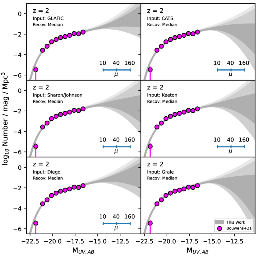
Figure 14.— The 68% and 95% likelihood contours (dark and light grey shaded regions, respectively) we derive on the shape of the $UV$ LFs at $z\sim 2$ based on our lensed HFF samples and the presented constraints on the LF from blank-field studies. Each panel shows the likelihood contours derived using one of six lensing v4 models as the truth in our forward-modeling procedure (Bouwens et al. 2017b) and then recover LF results using the median magnification from the other parametric lensing models. The light shaded regions shown here are similar to Figure 4. The blank-field constraints are from Bouwens et al. (2021a) and include essentially HST observations acquired to date over legacy fields.

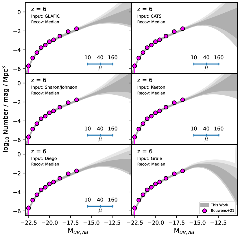
Figure 15.— Identical to Figure 14, but for $z\sim 6$ LF results.

Appendix B B. Sensitivity of faint-end slope determinations to the Probed $UV$ Luminosity Range

In deriving constraints on the faint-end slope $\alpha$ of the $UV$ LF from lensed sources behind the HFF clusters and comparing this slope with faint-end slope determinations derived from blank-field studies, an important question is how comparable these two faint-end slopes are. If the faint end of the $UV$ LF showed a modest departure from a power-law form, one would expect slight differences in the derived slopes.

To evaluate how large such differences might be, we make use of some of the model $UV$ LFs discussed in §4.4 and then characterize the differences in derived faint-end slope $\alpha$ based on the magnitude range over which the $UV$ LF is derived. For this exercise, faint-end slope determinations from blank-field and lensing cluster studies are assumed to occur from $-16.5$ mag to $-18.5$ mag and from $-18.0$ mag to $-15.0$ mag, respectively. In characterizing the impact that the luminosity range can have in deriving the faint-end slope $\alpha$, a characteristic luminosity $M_{UV}^{*}=-21$ is assumed and the impact that this would have on the power-law slope over the luminosity ranges described is removed ($\Delta\alpha\sim 0.02$).

Figure 16 shows the differences in the faint-end slope determinations depending on which luminosity range is utilized. The thick shaded line shows the median result. While there is a modest amount of scatter, model to model, the model results suggest LFs might show slightly shallower slopes, i.e., $\Delta\alpha\sim 0.0$-0.2 if probed from a lensing cluster study than from blank fields. Nevertheless, given how small the difference is and that it is dependent on which LF model we consider, we will not consider it further, but to note that a $\Delta\alpha\sim 0.1$ offset may be relevant for such a comparison.

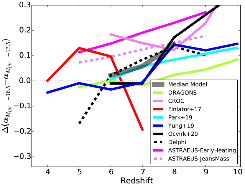
Figure 16.— Differences between the effective faint-end slope $\alpha$ of the $UV$ LF measured over the $UV$ luminosity range $M_{UV}$ $-18.0$ mag to $-15.0$ mag and over the range $M_{UV}$ $-18.5$ to $-16.5$ mag. The former luminosity range is more indicative of faint-end slope determinations from lensing cluster studies like the present one and the latter range is more indicative of determinations from blank-field studies that utilize HUDF samples (e.g., B21a). The presented results are based on the model LFs shown in Figures 12-13 and are shown as a function of redshift. The median difference $\Delta\alpha$ seen across all of the model LFs is shown as the thick shaded black line and appears to lie in the range $\sim 0.00$-0.15.

References

- Adams et al. (2020) Adams, N. J., Bowler, R. A. A., Jarvis, M. J., et al. 2020, MNRAS, 494, 1771
- Alavi et al. (2014) Alavi, A., Siana, B., Richard, J., et al. 2014, ApJ, 780, 143
- Alavi et al. (2016) Alavi, A., Siana, B., Richard, J., et al. 2016, ApJ, 832, 56
- Arnouts et al. (2005) Arnouts, S., Schiminovich, D., Ilbert, O., et al. 2005, ApJ, 619, L43
- Atek et al. (2014) Atek, H., Richard, J., Kneib, J.-P., et al. 2014, ApJ, 786, 60
- Atek et al. (2015) Atek, H., Richard, J., Kneib, J.-P., et al. 2015a, ApJ, 800, 18
- Atek et al. (2015) Atek, H., Richard, J., Jauzac, M., et al. 2015b, ApJ, 814, 69
- Atek et al. (2018) Atek, H., Richard, J., Kneib, J.-P., & Schaerer, D. 2018, MNRAS, 479, 5184
- Aubert & Teyssier (2008) Aubert, D. & Teyssier, R. 2008, MNRAS, 387, 295
- Barrow et al. (2017) Barrow, K. S. S., Wise, J. H., Norman, M. L., O’Shea, B. W., & Xu, H. 2017, MNRAS, 469, 4863
- Beckwith et al. (2006) Beckwith, S. V. W., Stiavelli, M., Koekemoer, A. M., et al. 2006, AJ, 132, 1729.
- Behroozi et al. (2013) Behroozi, P. S., Wechsler, R. H., & Conroy, C. 2013, ApJ, 770, 57
- Bhatawdekar et al. (2019) Bhatawdekar, R., Conselice, C. J., Margalef-Bentabol, B., et al. 2019, MNRAS, 486, 3805
- Bird et al. (2022) Bird, S., Ni, Y., Di Matteo, T., et al. 2022, MNRAS, 512, 3703
- Bouwens et al. (2007) Bouwens, R. J., Illingworth, G. D., Franx, M., & Ford, H. 2007, ApJ, 670, 928
- Bouwens et al. (2009) Bouwens, R. J., Illingworth, G. D., Franx, M., et al. 2009a, ApJ, 705, 936
- Bouwens et al. (2009) Bouwens, R. J., Illingworth, G. D., Bradley, L. D., et al. 2009b, ApJ, 690, 1764
- Bouwens et al. (2014) Bouwens, R. J., Illingworth, G. D., Oesch, P. A., et al. 2014, ApJ, 793, 115
- Bouwens et al. (2015) Bouwens, R. J., Illingworth, G. D., Oesch, P. A., et al. 2015a, ApJ, 803, 34
- Bouwens et al. (2015) Bouwens, R. J., Illingworth, G. D., Oesch, P. A., et al. 2015b, ApJ, 811, 140
- Bouwens (2016) Bouwens, R. 2016, Understanding the Epoch of Cosmic Reionization: Challenges and Progress, 423, 111
- Bouwens et al. (2016) Bouwens, R. J., Oesch, P. A., Labbé, I., et al. 2016a, ApJ, 830, 67
- Bouwens et al. (2016) Bouwens, R. J., Aravena, M., Decarli, R., et al. 2016b, ApJ, 833, 72
- Bouwens et al. (2017) Bouwens, R. J., Illingworth, G. D., Oesch, P. A., et al. 2017a, ApJ, 843, 41
- Bouwens et al. (2017) Bouwens, R. J., Oesch, P. A., Illingworth, G. D., et al. 2017b, ApJ, 843, 129
- Bouwens et al. (2017) Bouwens, R. J., Illingworth, G. D., Oesch, P. A., et al. 2017c, arXiv:1711.02090
- Bouwens et al. (2019) Bouwens, R. J., Stefanon, M., Oesch, P. A., et al. 2019, ApJ, 880, 25
- Bouwens et al. (2020) Bouwens, R., González-López, J., Aravena, M., et al. 2020, ApJ, 902, 112
- Bouwens et al. (2021) Bouwens, R. J., Oesch, P. A., Stefanon, M., et al. 2021a, AJ, 162, 47
- Bouwens et al. (2021) Bouwens, R. J., Illingworth, G. D., van Dokkum, P. G., et al. 2021b, AJ, 162, 255
- Bouwens et al. (2022a) Bouwens, R. J., Illingworth, G. D., van Dokkum, P. G., et al. 2022a, ApJ, 927, 81
- Bouwens et al. (2022b) Bouwens, R. J., Illingworth, G., Ellis, R. S., et al. 2022b, ApJ, 931, 81
- Bowler et al. (2015) Bowler, R. A. A., Dunlop, J. S., McLure, R. J., et al. 2015, MNRAS, 452, 1817
- Bowler et al. (2017) Bowler, R. A. A., Dunlop, J. S., McLure, R. J., & McLeod, D. J. 2017, MNRAS, 466, 3612
- Bowler et al. (2020) Bowler, R. A. A., Jarvis, M. J., Dunlop, J. S., et al. 2020, MNRAS, 493, 2059