Monomiality and a New Family of Hermite Polynomials

Abstract

In this article we go deeply into the formulation and meaning of the monomiality principle and employ it to study the properties of a set of polynomials, which, asymptotically, reduce to the ordinary two variable Kampè-dè-Fèrièt family. We derive the relevant differential equations and discuss the associated orthogonality properties, along with the relevant generalized forms.

Keywords
Special functions 33C52, 33C65, 33C99, 33B10, 33B15; Hermite polynomials 33C45; operators theory 44A99, 47B99, 47A62.

1 Introduction

The Hermite polynomials belong to the Appèll family [1] and the relevant properties can be conveniently framed within the context of the monomiality principle [2, 3]. This is a modern formulation of a point of view, tracing back to Steffensen [4, 5, 6], but even to older researches by Jeffery (for a recent account see Ref. [7]), Boole [8] and to other speculations developed almost two hundred years ago. These researches deepened their roots into the calculus of differences [9], the first to be recognized as amenable for a symbolic interpretation. The rules underlying monomiality are fairly simple and can be formulated as reported below [2, 3, 11, 12, 13]

Properties 1.

$\forall x\in\mathbb{R},\forall n\in\mathbb{N}$, If a couple of operators $\hat{P},\hat{M}$ are such that:

• they do exist along with a differential realization,

• they can be embedded to form a Weyl algebra [10, 14, 15], namely if commutator is such that $[\hat{P},\hat{M}]=\hat{1}$,

• it is possible to univocally define a polynomial set such that:

  $$i)\;p_{0}(x)=1,\qquad\qquad ii)\;\hat{P}p_{0}(x)=0,\qquad\qquad iii)\;p_{n}(x)=\hat{M}^{n}1,$$ (1)

then it follows that

• $$\hat{M}p_{n}(x)=\hat{M}^{n+1}1=p_{n+1}(x),$$ (2)

• $$\hat{P}p_{n}(x)=\hat{P}\hat{M}^{n}1=np_{n-1}(x)$$ (3)

and the polynomials $p_{n}(x)$ are said Quasi-Monomials.

Proof.

Eq. (3) needs few lines of comment. We rearrange the operator product $\hat{P}\hat{M}^{n}$ as (see [16])

$$\begin{split}\hat{P}\hat{M}\hat{M}^{n-1}&=(\hat{M}\hat{P}+1)\hat{M}^{n-1}=\hat{M}\hat{P}\hat{M}^{n-1}+\hat{M}^{n-1}=\\ &=\hat{M}^{2}\hat{P}\hat{M}^{n-2}+2\hat{M}^{n-1}=\dots=\hat{M}^{n}\hat{P}+n\hat{M}^{n-1},\end{split}$$ (4)

which eventually yields

$$\hat{P}\hat{M}^{n}1=\left(\hat{M}^{n}\hat{P}+n\hat{M}^{n-1}\right)1=\hat{M}^{n}\hat{P}\;1+n\hat{M}^{n-1}1.$$ (5)

Being $\hat{M}^{n}\hat{P}\;1=0$ as a consequence of the $ii)$ of Eqs. (1), and using property $iii)$ too, we state the correctness of Eq. (3). ∎

Remark 1.

The important point we like to convey is that the essence of the discussion on Monomiality is the existence of the operators $\hat{M}$ (multiplicative), which univocally define the set of polynomials $p_{n}(x)$ (not vice-versa), and $\hat{P}$ acting on the polynomials as an ordinary derivative.

According to the above statement polynomial set like Appèll, Sheffer [17], Boas Buck [18]…can be ascribed to the monomial family, while others like e. g. Legendre, Chebyshev, Jacobi…[19, 20] are not be framed within such a context.

After these remarks, aimed at clarifying the frame in which we are going to develop our speculations, we remind that the $\hat{M}$, $\hat{P}$ operators, defining the Appèl family, are defined by

$$\hat{M}=x+\dfrac{A^{\prime}(\sigma)}{A(\sigma)}\mid_{\sigma=\partial_{x}},\qquad\qquad\qquad\hat{P}=\partial_{x}\;,$$ (6)

where $A(\sigma)$ is an analytic function.

According to our introductory remarks, the explicit form of the Appèl polynomials is obtained from the identity (property $iii)$ of Eq. (1))

$$a_{n}(x)=\left(x+\dfrac{A^{\prime}(\partial_{x})}{A(\partial_{x})}\right)^{n}1.$$ (7)

The use of standard operational rules allows to cast Eq. (7) in a more convenient form.

Corollary 1.

We note indeed that [21, 22]

$$a_{n}(x)=\left(x+\dfrac{A^{\prime}(\partial_{x})}{A(\partial_{x})}\right)\left(x+\dfrac{A^{\prime}(\partial_{x})}{A(\partial_{x})}\right)^{n-1}1$$ (8)

and noting that

$$x+\dfrac{A^{\prime}(\partial_{x})}{A(\partial_{x})}=A(\partial_{x})x\left(A(\partial_{x})\right)^{-1},$$ (9)

we can write, by iteration

$$a_{n}(x)=\left(A(\partial_{x})x\left(A(\partial_{x})\right)^{-1}\right)^{n}=A(\partial_{x})x^{n}$$ (10)

Acording to Eq. (10), the generating function of Appèl polynomials reads

$$\sum_{n=0}^{\infty}\dfrac{t^{n}}{n!}a_{n}(x)=A(\partial_{x})e^{tx}=A(t)e^{tx}.$$ (11)

It is evident that it consists of two contributions: the exponential term and $A(t)$, which will be defined as the “amplitude”.

Corollary 2.

In the case of the two variable Hermite polynomials ($HP$), we have that the amplitude is specified by

$$A(t)=e^{yt^{2}}$$ (12)

with the multiplicative operator being explicitly defined by

$$\hat{M}=x+2y\partial_{x}\;.$$ (13)

The associated polynomial family is, accordingly, provided by [26]

$$H_{n}(x,y)=(x+2y\partial_{x})^{n}1.$$ (14)

The use of the Crofton identity [23]

$$e^{y\partial_{x}^{m}}f(x)=f\left(x+m\;y\;\partial_{x}^{m-1}\right)e^{y\partial_{x}^{m}}$$ (15)

(or of identities (10)-(11) as well) allows to cast Eq. (14) in the form

$$H_{n}(x,y)=e^{y\partial_{x}^{2}}x^{n}.$$ (16)

The expansion of the exponential operator in Eq. (16), along with the relevant action on the monomial $x^{n}$, yields the explicit form of the two variable Hermite polynomials [10, 1], namely

$$H_{n}(x,y)=n!\sum_{r=0}^{\lfloor\frac{n}{2}\rfloor}\dfrac{x^{n-2r}y^{r}}{(n-2r)!r!}.$$ (17)

The operational identity in Eq. (16) is particularly pregnant from the mathematical point of view. It states that the two variable Hermite (17) are solutions of the heat equation and can be used as a pivotal tool to prove the orthogonal properties of this polynomial family [10, 26].

In this article we consider the polynomial family generated by

$$A(p)=\left(1+\dfrac{y}{N}p^{2}\right)^{N},\qquad\forall N\in\mathbb{N},$$ (18)

study the relevant properties and look at the possibility of defining an associated orthogonal set.

2 Quasi-Hermite and Appéll Sequences

In this section we exploit the general properties of the Appéll polynomials, discussed in the introductory remarks, to state the properties of the associated polynomials.

Definition 1.

Appéll polynomials with amplitude (18), are explicitly defined through the identity

$$H_{n}(x,y;N)=\left(1+\dfrac{y}{N}\partial_{x}^{2}\right)^{N}x^{n}$$ (19)

and they will be called Quasi-Hermite-Polynomials ($QHP$) .

Properties 2.

The relevant recurrences of $QHP$ are obtained after noting that, for this specific case, we get

$$\dfrac{A^{\prime}(\partial_{x})}{A(\partial_{x})}=\dfrac{2\;y\;\partial_{x}}{\left(1+\dfrac{y}{N}\partial_{x}^{2}\right)},$$ (20)

so

$$\begin{split}&1)\;\partial_{x}H_{n}(x,y;N)=n\left(1+\dfrac{y}{N}\partial_{x}^{2}\right)^{N}x^{n-1}=nH_{n-1}(x,y;N),\\ &2)\;H_{n+1}(x,y;N)=\left(x+\dfrac{2\;y\;\partial_{x}}{1+\frac{y}{N}\partial_{x}^{2}}\right)H_{n}(x,y;N),\\ &3)\;H_{n+1}(x,y;N)-xH_{n}(x,y;N)-2nyH_{n-1}(x,y;N)=\\ &=\dfrac{y}{N}n(n-1)\left(xH_{n-2}(x,y;N)-H_{n-1}(x,y;N)\right).\end{split}$$ (21)

Proof.

Properties $1)$ and $2)$ are obtained from the realization of the derivative and multiplicative operators given in Eqs. (6). About the third one, it is the result of some algebraic steps:

• From property $2)$ we write

  $$\left(1+\dfrac{y}{N}\partial_{x}^{2}\right)H_{n+1}=\left(1+\dfrac{y}{N}\partial_{x}^{2}\right)xH_{n}+2y\partial_{x}H_{n}$$

  which provides, from property $1)$,

• $$H_{n+1}+\dfrac{y}{N}n(n+1)H_{n-1}=xH_{n}+\dfrac{y}{N}\left(2nH_{n-1}+n(n-1)xH_{n-2}\right)+2nyH_{n-1}$$

  and finally

• $$\begin{split}H_{n+1}-xH_{n}-2nyH_{n-1}&=\dfrac{y}{N}n\left(\left(2-(n+1)\right)H_{n-1}+(n-1)xH_{n-2}\right)=\\ &=\dfrac{y}{N}n(n-1)\left(xH_{n-2}-H_{n-1}\right).\end{split}$$

∎

Proposition 1.

The explicit form of the $QHP$ is inferred from Eq. (19), which yields

$$a)\;H_{n}(x,y;N)=\sum_{r=0}^{\min\left[N,\;\lfloor\frac{n}{2}\rfloor\right]}\binom{N}{r}\left(\dfrac{y}{N}\right)^{r}\dfrac{n!}{(n-2r)!}x^{n-2r},\quad\forall x,y\in\mathbb{R},\forall n,N\in\mathbb{N}$$ (22)

and the relevant differential equation is

$$b)\;\left(x+\dfrac{2\;y\;\partial_{x}}{1+\frac{y}{N}\partial_{x}^{2}}\right)\partial_{x}H_{n}(x,y;N)=nH_{n}(x,y;N).$$ (23)

Proof.

a) $\forall x,y\in\mathbb{R},\forall n,N\in\mathbb{N}$, we use binomial Newton to write

$$H_{n}(x,y;N)=\sum_{r=0}^{N}\binom{N}{r}\left(\dfrac{y}{N}\right)^{r}\partial_{x}^{2r}x^{n}=\sum_{r=0}^{\min\left[N,\;\lfloor\frac{n}{2}\rfloor\right]}\binom{N}{r}\left(\dfrac{y}{N}\right)^{r}\dfrac{n!}{(n-2r)!}x^{n-2r}.$$

b) The relevant differential equation is easily obtained by applying Eqs. (21) in Properties 2. ∎

Corollary 3.

After a few algebraic manipulations, Eq. (23) can be reduced to the following third order $ODE$

$$\dfrac{y}{N}xz^{{}^{\prime\prime\prime}}+y\left(2-\dfrac{n-2}{N}\right)z^{{}^{\prime\prime}}+xz^{\prime}=nz,\qquad\qquad z=H_{n}(x,y;N)$$ (24)

which, evidently, tends to the ordinary (two variables) Hermite equation, for large $N$ values.

Proof.

By starting from Eq. (23) we write

$$\begin{split}&\left(\left(1+\dfrac{y}{N}\partial_{x}^{2}\right)x+2y\partial_{x}\right)\partial_{x}z=\left(1+\dfrac{y}{N}\partial_{x}^{2}\right)nz\quad\rightarrow\\ \rightarrow\;&\;x\partial_{x}z+\dfrac{y}{N}\partial_{x}^{2}x\partial_{x}z+2y\partial_{x}^{2}z=nz+\dfrac{y}{N}\partial_{x}^{2}nz\quad\rightarrow\\ \rightarrow\;&\;xz^{\prime}+\dfrac{y}{N}\partial_{x}(z^{\prime}+xz^{\prime\prime})+2yz^{\prime\prime}-\dfrac{y}{N}nz^{\prime\prime}=nz\quad\rightarrow\\ \rightarrow\;&\;\dfrac{y}{N}xz^{{}^{\prime\prime\prime}}+y\left(2-\dfrac{n-2}{N}\right)z^{{}^{\prime\prime}}+xz^{\prime}=nz\end{split}$$

∎

Corollary 4.

The $PDE$ satisfied by the $QHP$ (expected to be an extension of the heat equation) is obtained by keeping the partial derivative with respect to y of both sides of Eq. (19), namely

$$\partial_{y}H_{n}(x,y;N)=\partial_{x}^{2}\left(1+\dfrac{y}{N}\partial_{x}^{2}\right)^{N-1}x^{n}.$$ (25)

Example 1.

Eq. (25) can eventually be written as

$$\left\{\begin{array}[]{l}\partial_{y}H_{n}(x,y;N)=\dfrac{\partial_{x}^{2}}{1+\frac{y}{N}\partial_{x}^{2}}H_{n}(x,y;N)\\[4.73611pt] H_{n}(x,0;N)=x^{n}\end{array}\right.$$ (26)

The relevant (formal) solution can be obtained as

$$H_{n}(x,y;N)=\hat{U}_{y,N}\;x^{n},\qquad\qquad\hat{U}_{y,N}=\exp\left\{\int_{0}^{y}\dfrac{\partial_{x}^{2}}{1+\frac{\xi}{N}\partial_{x}^{2}}\;d\xi\right\},$$ (27)

where $\hat{U}$ is a kind of evolution operator. To be eventually written as in Eq. (19), after explicitly working out the integral in the exponent of Eq. (27), we find

$$\hat{U}_{y,N}=\exp\left\{N\log\left(1+\dfrac{y}{N}\partial_{x}^{2}\right)\right\}=\left(1+\dfrac{y}{N}\partial_{x}^{2}\right)^{N}.$$ (28)

According to the previous definition, the $QHP$ satisfies the composition rule

$$\hat{U}_{y,N}\hat{U}_{z,N}=\left(1+\dfrac{y+z}{N}\partial_{x}^{2}+\dfrac{yz}{N^{2}}\partial_{x}^{4}\right)^{N}.$$ (29)

Therefore, unlike the two variables $HP$ specified by an amplitude that is an exponential , the composition property $\hat{U}_{y,N}\hat{U}_{z,N}=\hat{U}_{y+z,N}$ does not hold, therefore

$$\hat{U}_{y,N}\hat{U}_{z,N}\neq\hat{U}_{y+z;N}.$$ (30)

An important (albeit naïve) consequence of Eq. (29) is the following composition rule

$$\hat{U}_{-y,N}\hat{U}_{y,N}x^{n}=\left(1-\dfrac{y^{2}}{N^{2}}\partial_{x}^{4}\right)^{N}x^{n},$$ (31)

which suggests the necessity of a suitable extension of $QHP$, possibly involving higher order forms, as discussed in the forthcoming section.

Observation 1.

The non exponential nature of the $QHP$ amplitude determines the further worth to be noted consequence

$$\hat{U}_{-y,N}\neq\hat{U}_{y,N}^{-1}=\dfrac{1}{\Gamma(N)}\int_{0}^{\infty}s^{N-1}e^{-s\left(1+\frac{y}{N}\partial_{x}^{2}\right)}ds,$$ (32)

where the r.h.s. has been obtained after exploiting standard Laplace transform methods.

We will see in the following that Eq. (32) is of pivotal importance for the definition of the orthogonal properties of the $QHP$.

Observation 2.

Before closing this section, we notice that Eq. (23) can be generalized $\forall m\in\mathbb{N}$ such that

$$\left(x+\dfrac{m\;y\;\partial^{m-1}_{x}}{1+\frac{y}{N}\partial_{x}^{m}}\right)\partial_{x}H^{(m)}_{n}(x,y;N)=nH^{(m)}_{n}(x,y;N).$$ (33)

and, by following the same procedure provided in the Corollary 3, it is possible to deduce the relative differential equantion.

3 Multivariable $QHP$

Higher order Hermite polynomials (also called Lacunary HP) are defined through the operational rule [10, 23]

$$H_{n}^{(m)}(x,y)=e^{y\partial_{x}^{m}}x^{n},\qquad\quad\forall m\in\mathbb{N}$$ (34)

and, in analogy, the Higher order $QHP$ are specified by

$$H^{(m)}_{n}(x,y;N)=\hat{U}^{(m)}_{y,N}\;x^{n},\qquad\qquad\hat{U}^{(m)}_{y,N}=\left(1+\dfrac{y}{N}\partial_{x}^{m}\right)^{N}.$$ (35)

Example 2.

According to Eq. (31), we find

$$\hat{U}_{-y,N}\hat{U}_{y,N}\;x^{n}=\hat{U}^{(4)}_{-y^{2},N}\;x^{n}=H_{n}^{(4)}\left(x,-y^{2};N\right)$$ (36)

and, more in general,

$$\hat{U}^{(m)}_{-y,N}\hat{U}^{(m)}_{y,N}x^{n}=\hat{U}^{(2m)}_{-y^{2},N}\;x^{n}=H_{n}^{(2m)}\left(x,-y^{2};N\right)$$ (37)

Example 3.

Before going further, we consider the definition of the $QHP$ of order one, which will be referred as Quasi Binomial Polynomials ($QBP$), namely

$$H_{n}^{(1)}(x,y;N)=\left(1+\dfrac{y}{N}\partial_{x}\right)^{N}x^{n}.$$ (38)

For large $N$ they reduce to $(x+y)^{n}$ hence the name. The explicit form of this family of polynomials, writes

$$H_{n}^{(1)}(x,y;N)=\sum_{r=0}^{N}\binom{N}{r}\left(\dfrac{y}{N}\right)^{r}\partial_{x}^{r}x^{n}=\sum_{r=0}^{\min\left[N,\;n\right]}\binom{N}{r}\left(\dfrac{y}{N}\right)^{r}\dfrac{n!}{(n-r)!}x^{n-r}.$$ (39)

The same strategy adopted in Corollary 3, by exploiting Eq. (33), yields for the $QBP$ the $ODE$

$$\dfrac{y}{N}xz^{{}^{\prime\prime}}+\left[(x+y)-(n-1)\dfrac{y}{N}\right]z^{\prime}=nz,\qquad\qquad z=H_{n}^{(1)}(x,y;N)$$ (40)

and the $PDE$

$$\left\{\begin{array}[]{l}\partial_{y}F(x,y)=\dfrac{\partial_{x}}{1+\frac{y}{N}\partial_{x}}F(x,y)\\[5.16663pt] F(x,0)=x^{n}\end{array}.\right.$$ (41)

The last identity can also be cast in the integro-differential form

$$\partial_{y}F(x,y)=\partial_{x}\int_{0}^{\infty}e^{-s}F\left(x-\dfrac{y}{N}s,\;y\right)ds$$ (42)

indeed, the Laplace transform provides the integral representation

$$\dfrac{1}{1+\frac{y}{N}\partial_{x}}=\int_{0}^{\infty}e^{-s\left(1+\frac{y}{N}\partial_{x}\right)}ds$$ (43)

which, one inserted in Eq. (41), yields

$$\partial_{y}F(x,y)=\partial_{x}\int_{0}^{\infty}e^{-s}e^{-\frac{ys}{N}\partial_{x}}dsF(x,y)$$ (44)

and, after exploiting the shift operator identity $e^{a\partial_{x}}f(x)=f(x+a)$ [10], we obtain Eq. (42).

Example 4.

We can combine the various definition given before to introduce three variables $QHP$ as

$$\begin{split}H_{n}^{(1,2)}(x,y_{1},y_{2};N):&=\left(\hat{U}_{y_{1},N}^{(1)}\;\hat{U}_{y_{2},N}^{(2)}\right)x^{n}=\left(1+\dfrac{y_{1}}{N}\partial_{x}\right)^{N}\left(1+\dfrac{y_{2}}{N}\partial_{x}^{2}\right)^{N}x^{n}=\\ &=\left(1+\dfrac{y_{1}}{N}\partial_{x}\right)^{N}H_{n}(x,y_{2};N)=\\ &=n!\sum_{r=0}^{\min\left[N,n\right]}\binom{N}{r}\left(\dfrac{y_{1}}{N}\right)^{\!r}\dfrac{H_{n-r}(x,y_{2};N)}{(n-r)!}.\end{split}$$ (45)

Further generalizations can easily be obtained. For example the $m$-th variable extension reads

$$H_{n}^{(1,\dots,m)}(x,y_{1},\dots,y_{m};N)=\left(\prod_{s=1}^{n}\hat{U}_{y_{s},N}^{(s)}\right)x^{n}.$$ (46)

The examples we have just touched on in this section yields an idea of the possible extensions of this family of polynomials, which will be more carefully discussed in a forthcoming research.

4 Final Comments

We have already mentioned the possible orthogonal nature of the $QHP$, in this section we address the problem by the use of the techniques developed in Refs. [24, 25].

Proposition 2.

We assume that a given function $f(x)$ can be expanded in terms of $QHP$, according to the identity

$$f(x)=\sum_{n=0}^{\infty}a_{n}H_{n}(x,-\mid y\mid;N)$$ (47)

which can be inverted, thus yielding

$$\dfrac{1}{\left(1-\dfrac{\mid y\mid}{N}\partial_{x}^{2}\right)^{N}}\;f(x)=\sum_{n=0}^{\infty}a_{n}x^{n}.$$ (48)

The use of Eq. (32) allows to cast the l.h.s. of Eq. (48) in the form

$$\dfrac{1}{\Gamma(N)}\int_{0}^{\infty}s^{N-1}e^{-s\left(1-\frac{\mid y\mid}{N}\partial_{x}^{2}\right)}ds\;f(x)=\sum_{n=0}^{\infty}a_{n}x^{n}.$$ (49)

Corollary 5.

Eq. (49) can be so further elaborated:

1. We apply the Gauss-Weierstrass transform [26] to write

   $$\begin{split}e^{s\frac{\mid y\mid}{N}\partial_{x}^{2}}f(x)&=\dfrac{1}{2\sqrt{\pi\;s\frac{\mid y\mid}{N}}}\int_{-\infty}^{\infty}\exp\left\{-\dfrac{(x-\xi)^{2}}{4\;s\frac{\mid y\mid}{N}}\right\}f(\xi)d\xi=\\ &\;=\dfrac{1}{2\sqrt{\pi\;s\frac{\mid y\mid}{N}}}\int_{-\infty}^{\infty}e^{-\frac{1}{4\;s\frac{\mid y\mid}{N}}\xi^{2}}e^{\frac{x}{2s\frac{\mid y\mid}{N}}\xi}e^{-\frac{x^{2}}{4s\frac{\mid y\mid}{N}}}d\xi.\end{split}$$ (50)

   It holds for $s\frac{\mid y\mid}{N}\geq 0$ (hence the choice of the sign in the expansion (47)).
   

2. We use the two variable Hermite generating function [10] to write

   $$e^{s\frac{\mid y\mid}{N}\partial_{x}^{2}}f(x)=\dfrac{1}{2\sqrt{\pi\;s\frac{\mid y\mid}{N}}}\sum_{n=0}^{\infty}\dfrac{x^{n}}{n!}\int_{-\infty}^{\infty}H_{n}\left(\dfrac{\xi}{2s\frac{\mid y\mid}{N}},-\dfrac{1}{4s\frac{\mid y\mid}{N}}\right)e^{-\frac{\xi^{2}}{4\;s\frac{\mid y\mid}{N}}}f(\xi)d\xi.$$ (51)

3. We insert the result of Eq. (51), in Eq. (49) and compare the like $x$ powers, thus eventually finding

   $$\begin{split}&a_{n}=\dfrac{1}{\Gamma(N)n!\;2\sqrt{\pi\dfrac{\mid y\mid}{N}}}\int_{0}^{\infty}s^{N-\frac{3}{2}}e^{-s}\;{}_{n}G_{y,N}(s)ds,\\ &{}_{n}G_{y,N}(s)=\int_{-\infty}^{\infty}H_{n}\left(\dfrac{\xi}{2s\frac{\mid y\mid}{N}},-\dfrac{1}{4s\frac{\mid y\mid}{N}}\right)e^{-\frac{\xi^{2}}{4\;s\frac{\mid y\mid}{N}}}f(\xi)d\xi.\end{split}$$ (52)

According to the above results the expansion holds only if the integrals appearing in Eq. (52) are converging. In order to provide an example we consider the generalization of the Glaisher formula [27]. Namely Eq. (48), for $f(x)=e^{-x^{2}}$, becomes

$$\begin{split}F(x,y;N)&=\dfrac{1}{\left(1-\dfrac{\mid y\mid}{N}\partial_{x}^{2}\right)^{N}}f(x)=\dfrac{1}{\Gamma(N)}\int_{0}^{\infty}s^{N-1}e^{-s\left(1-\frac{\mid y\mid}{N}\partial_{x}^{2}\right)}e^{-x^{2}}ds=\\ &=\dfrac{1}{\Gamma(N)}\int_{0}^{\infty}s^{N-1}e^{-s}\dfrac{e^{-\frac{x^{2}}{1+4\frac{\mid y\mid}{N}s}}}{\sqrt{1+4\dfrac{\mid y\mid}{N}s}}\;ds.\end{split}$$ (53)

For very large $N$,  $\frac{1}{\left(1-\frac{\mid y\mid}{N}\partial_{x}^{2}\right)^{N}}e^{-x^{2}}$, reduces to the ordinary Glaisher identity

$$\lim\limits_{N\rightarrow\infty}F(x,y;N)=e^{\mid y\mid\partial_{x}^{2}}e^{-x^{2}}=\dfrac{1}{\sqrt{1+4y}}e^{-\frac{x^{2}}{1+4y}}.$$ (54)

In Figs. 1 we have reported $F(x,y;N)$ vs. $x$ for different values of $N$ and $y$.

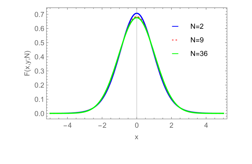
(a) $y=0.3$

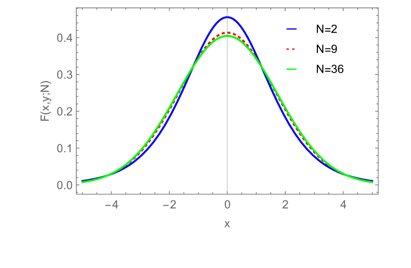
(b) $y=1.3$

Figure 1: $F(x,y;N)$ vs. $x$ for different values of $N$ and $y$

The definition of higher order ($QHP$) is not unique and another possibility is offered by the relation

$$H_{n}^{(q,p)}(x,y,z;N)=\left(1+\dfrac{y}{N}\partial_{x}^{q}+\dfrac{z}{N}\partial_{x}^{p}\right)^{N}x^{n}$$ (55)

where $q<p$ are relatively prime integers. The definition in Eq. (55) allows to write the composition identity (29) as

$$\hat{U}_{y,N}\hat{U}_{z,N}x^{n}=H_{n}^{(2,4)}\left(x,y+z,yz;N\right)^{N}\;x^{n}.$$ (56)

In this paper we have gone through different aspects of the theory of Hermite polynomials, which has allowed the introduction of a family of Quasi Hermite polynomials. The relevant properties have been studied with the help of the formalism of Monomiality.

In a forthcoming paper we will extend the present analysis to the definition of two variables Quasi Laguerre polynomials.

Acknowledgements
The work of Dr. S. Licciardi was supported by an Enea Research Center individual fellowship and under the auspices of INDAM’s GNFM (Italy).

References

• [1] Appéll, P.; Kampé de Fériét, J. Fonctions Hypergeometriques and Hyperspheriques. Polynomes d’Hermite, Gauthiers-Villars, Paris, 1926.
• [2] Bell, E.T. The History of Blissard’s Symbolic Method, with a Sketch of its Inventor’s Life, The American Mathematical Monthly, 45(7), 1938, pp. 414–421.
• [3] Dattoli, G. Generalized polynomials, operational identities and their applications, J. Comput. Appl. Math., 118(12), Elsevier, 2000, pp. 111–123.
• [4] J.F. Steffensen, Interpolation, The Williams & Wilkins Company , Baltimore, 1927.
• [5] J.F. Steffensen, On the definition of the central factorial, J. Inst. Actuaries, 64, 1933, pp. 165–168.
• [6] J.F. Steffensen, The poweroid, an extension of the mathematical notion of power, Acta Mathematica, 73, 1941, pp. 333–366.
• [7] Dowker, J.S. Poweroids revisited - an old symbolic approach, arXiv:1307.3150 [math.CO], 2013.
• [8] Boole, G. Calculus of Finite Differences, 2nd Edn., MacMillan, Cambridge, 1872.
• [9] Jordan, C. Calculus of finite differences, 3rd ed., AMS Chelsea, 1965.
• [10] Babusci, D., Dattoli, G., Licciardi, S., Sabia, E. Mathematical Methods for Physics, World Scientific, Singapore, 2019.
• [11] Dattoli, G. Generalized polynomials, operational identities and their applications, J. Comput. Appl. Math., Elsevier, vol. 118, Issues 12, 2000, pp. 111–123.
• [12] Dattoli, G. Hermite-Bessel and Laguerre-Bessel functions: a by-product of the monomiality principle, Advanc. Special Funct. Applic. (Melfi, 1999)– (D. Cocolicchio, G. Dattoli and H.M. Srivastava, Editors), Aracne Editrice, Rome, 2000, pp. 147–164.
• [13] Dattoli, G. Laguerre and generalized Hermite polynomials: the point of view of the operational method, Int. Trans. Spec. Funct., vol. 15(2), 2004.
• [14] Dattoli, G., Gallardo, J.C., Torre, A. An Algebraic View to the Operatorial Ordering and its Applications to Optics, Riv. Nuovo Cimento, 3(11), 1988, pp. 1–79.
• [15] Dattoli, G., Ottaviani, P.L., Torre, A., Vazquez, L. Evolution operator equations-integration with algebraic and finite-difference methods-applications to physical problems in classical and quantum mechanics and quantum field theory, Riv. Nuovo Cimento, 20(1), 1997.
• [16] Louisell, W.H. Quantum Statistical Properties of Radiation, John Wiley and Sons, 1973, Chapter 2.
• [17] Sheffer, I.M. Some Properties of Polynomial Sets of Type Zero, Duke Mathematical J., 5(3), 1939, pp. 590–622.
• [18] R.P. Boas, R.C. Buck, Polynomial expansions of analytic functions, Ergebnisse der Mathematik und ihrer Grenzgebiete. Neue Folge., 19, Berlin, New York: Springer-Verlag, MR 0094466, (1958).
• [19] Andrews, L.C. ”Special Functions For Engeneers and Applied mathematicians”, Mc Millan New York, 1985.
• [20] Abramovitz M, Stegun IA. ”Handbook of Mathematical Functions with Formulas, Graphs and Mathematical Tables”, 9th printing, Dover, New York, 1972,
• [21] Dattoli, G., Germano, B., Martinelli, M.R., Ricci, P.E. Sheffer and Non-Sheffer Polynomial Families, Intern. J. Math. and Mathem. Sc., Hindawi Publishing Corporation, 2012, Article ID 323725, 8 pages, doi:10.1155/2012/323725.
• [22] Dattoli, G., Zhukovsky, K. Appél Polynomial Series Expansions, Intern. Mathem. Forum, 5, no. 14, 2010, pp. 649–662.
• [23] Dattoli, G., Khan, S., Ricci, P.E. On Crofton-Glaisher type relations and derivation of generating functions for Hermite polynomials including the multi-index case, Int. Transf. Spec. Funct., 19(1), 2008, pp. 1–9.
• [24] Dattoli, G., Germano, B., Ricci, P.E. Comments on monomiality, ordinary polynomials and associated bi-orthogonal functions, Appl. Math. Comput., 154, 2004, pp. 219–227.
• [25] Dattoli, G., Germano, B., Ricci, P.E. Hermite polynomials with more than two variables and associated bi-orthogonal functions, Integr. Transf. Spec. Funct., vol. 20, no. 1, 2009, pp. 17–22.
• [26] Licciardi, S. Umbral Calculus, a Different Mathematical Language, PhD Thesis, Dep. of Mathematics and Computer Sciences, XXIX cycle, University of Catania, 2018.
• [27] Dattoli, G., Khan, S., Ricci, P.E. On Crofton-Glaisher type relations and derivation of generating functions for Hermite polynomials including the multi-index case, Integr. Transf. Spec.Funct., 19 (1), 2008, pp. 1–9.