Robust multiscale estimation of time-average variance for time series segmentation

Abstract

There exist several methods developed for the canonical change point problem of detecting multiple mean shifts, which search for changes over sections of the data at multiple scales. In such methods, estimation of the noise level is often required in order to distinguish genuine changes from random fluctuations due to the noise. When serial dependence is present, using a single estimator of the noise level may not be appropriate. Instead, it is proposed to adopt a scale-dependent time-average variance constant that depends on the length of the data section in consideration, to gauge the level of the noise therein. Accordingly, an estimator that is robust to the presence of multiple mean shifts is developed. The consistency of the proposed estimator is shown under general assumptions permitting heavy-tailedness, and its use with two widely adopted data segmentation algorithms, the moving sum and the wild binary segmentation procedures, is discussed. The performance of the proposed estimator is illustrated through extensive simulation studies and on applications to the house price index and air quality data sets.

Keywords: change point analysis, time-average variance constant, robust estimation, moving sum procedure, wild binary segmentation

1 Introduction

Dating back to the 1950s (Page,, 1954), change point analysis has a long tradition in statistics. The area continues to be an active field of research due to its importance in many applications where data is routinely collected in highly nonstationary environments. Data segmentation, a.k.a. multiple change point detection, enables partitioning of a time series into stationary regions and thus provides a simple framework for modelling nonstationary time series.

We consider the problem of detecting multiple change points in the piecewise constant mean of an otherwise stationary time series. We briefly review the existing literature on multiple change point detection in the presence of serial dependence, and refer to Aue and Horváth, (2013) and Truong et al., (2020) for a comprehensive overview. One line of research takes a parametric approach and simultaneously estimates the serial dependence and change points. For example, Chakar et al., (2017), Fang and Siegmund, (2020) and Romano et al., (2021) assume an autoregressive (AR) model of order one, while Lu et al., (2010), Cho and Fryzlewicz, (2021) and Gallagher et al., (2022) permit an AR model of arbitrary order.

Another line of research focuses on extending the use of the methodologies developed for independent data to time series settings. Lavielle and Moulines, (2000) and Cho and Kirch, (2021) adopt information criteria originally developed for a sequence of independent, Gaussian random variables (Yao,, 1988), to data exhibiting serial correlations and heavy tails, which requires the choice of an appropriate penalty that depends on the tail behaviour of noise. Tecuapetla-Gómez and Munk, (2017), Eichinger and Kirch, (2018), Dette et al., (2020) and Chan, (2022) propose estimators of the long-run variance (LRV) for quantifying the level of noise that are robust to the presence of multiple mean shifts. We also note that Wu and Zhou, (2020) and Zhao et al., (2021) extend self-normalisation-based change point tests to the data segmentation problem.

In this paper, we propose a robust estimator of the scale-dependent time-average variance constant (TAVC, Wu,, 2009). It is closely related to the literature on estimation of the LRV, namely $\sigma^{2}=\lim_{N\to\infty}\mathsf{Var}(N^{-1/2}\sum_{t=1}^{N}\varepsilon_{t})$ for a stationary time series $\{\varepsilon_{t}\}_{t\in\mathbb{Z}}$, but distinct in that our interest lies in estimating

$$\sigma^{2}_{L}=\mathsf{Var}\left(\frac{1}{\sqrt{L}}\sum_{t=1}^{L}\varepsilon_{t}\right),$$ (1)

for a given scale $L$. We argue that such a scale-dependent TAVC estimator is well-suited to be combined with a class of multiscale change point detection methodologies, examples of which include the moving sum (MOSUM) procedure (Eichinger and Kirch,, 2018) and the wild binary segmentation (WBS, Fryzlewicz,, 2014) algorithm. Such approaches locally apply change point tests for single change point detection, to data sections of varying lengths and achieve good adaptivity in multiple change point detection (Cho and Kirch,, 2021). We motivate the use of scale-dependent TAVC in (1) in combination with such multiscale methods in the following examples.

Example 1.

Consider an MA($1$) process $\varepsilon^{(1)}_{t}=W_{t}-0.9W_{t-1}$ and an AR($1$) process $\varepsilon^{(2)}_{t}=0.9\varepsilon^{(2)}_{t-1}+W_{t}$, where $\{W_{t}\}_{t\in\mathbb{Z}}$ is a white noise process with $\mathsf{Var}(W_{t})=1$. Figure 1 shows the TAVC of $\{\varepsilon^{(1)}_{t}\}_{t\in\mathbb{Z}}$ and $\{\varepsilon^{(2)}_{t}\}_{t\in\mathbb{Z}}$ for increasing $L$, along with the true LRV, which highlights the large gap between $\sigma^{2}_{L}$ and $\sigma^{2}$ particularly at a small scale $L$. This discrepancy has an impact on the performance of change point detection methods.

Figure 2 further illustrates this point by plotting the MOSUM detector statistics generated with a moving window of length $30$ (see Equation (11) for its definition), on the data generated by adding $\{\varepsilon^{(1)}_{t}\}_{t=1}^{n}$ and $\{\varepsilon^{(2)}_{t}\}_{t=1}^{n}$ to a piecewise signal with two change points at times $\tau_{1}=200$ and $\tau_{2}=260$, respectively ($n=1000$). Then, the detector statistics are scaled by the proposed estimator of TAVC (solid) and the true LRV (dashed). For accurate detection of the change points, we expect that a sequence of appropriately scaled detector statistics forms two prominent peaks at the change points that exceed a theoretically motivated threshold, while away from the change points, detector statistics remain below the threshold, see Section 3.1 for further details. In combination with the TAVC estimator, the detector statistics exhibit the desired behaviour such that both change points are detectable from the scaled MOSUM statistics. However, due to the lack of adaptivity of the LRV to the scale-dependent variability of the detector statistics, its use leads to either a large number of false positives (spurious peaks above threshold, see the top panel of Figure 2), or false negatives (MOSUM detector statistics scaled by the LRV do not exceed the threshold near $\tau_{i},\,i=1,2$, see the bottom panel of Figure 2).

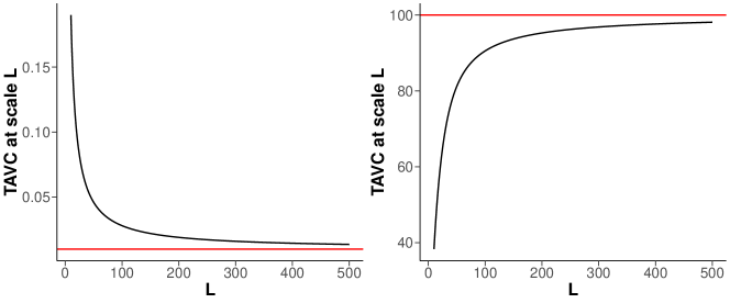
Figure 1: TAVC $\sigma^{2}_{L}$ for increasing $L$ (black line) computed on the MA(1) process $\varepsilon^{(1)}_{t}=W_{t}-0.9W_{t-1}$ (left) and the AR(1) process $\varepsilon^{(2)}_{t}=0.9\varepsilon^{(2)}_{t-1}+W_{t}$ (right). The respective LRV is given by the horizontal red line.

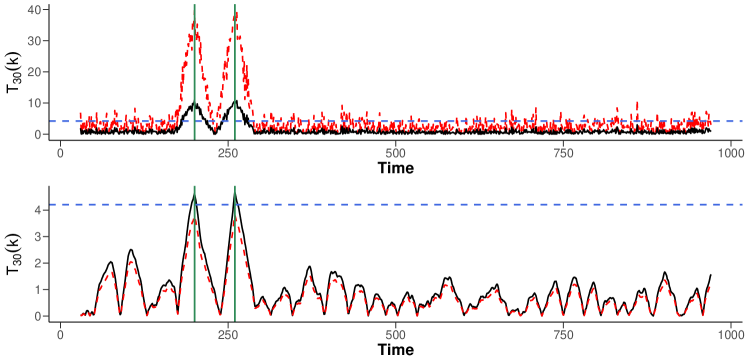
Figure 2: Scaled MOSUM detector statistics computed on the data generated by adding $\{\varepsilon^{(1)}_{t}\}_{t=1}^{n}$ (top) and $\{\varepsilon^{(2)}_{t}\}_{t=1}^{n}$ (bottom), to a piecewise constant signal with two change points ($n=1000$, green vertical lines denote the true change locations). The detector statistics scaled by the proposed TAVC estimator (black solid line) and true LRV (red dashed line) are plotted. Dashed blue horizontal line denotes a theoretically motivated threshold at $5$% significance level.

Example 1 demonstrates that adopting the global LRV may fail to reflect the degree of variability in the local data sections that are used in computing change point detector statistics adopted by multiscale data segmentation algorithms, which in turn may result in false negatives or positives. Moreover, when the LRV is close to zero as in the case of $\{\varepsilon^{(1)}_{t}\}_{t\in\mathbb{Z}}$ in Example 1, some estimators of the LRV have been observed to take negative values (Hušková and Kirch,, 2010), which further makes their use in change point problems undesirable.

To ensure that the scale-dependent TAVC estimator is robust to the mean shifts, we adopt the robust $M$-estimation framework of Catoni, (2012), which was first proposed in the independent setting for mean and variance estimation and further extended to the serially dependent setting for LRV estimation in Chen et al., (2021). We establish the consistency of the proposed robust estimator of scale-dependent TAVC under general conditions permitting heavy tails and serial dependence decaying at a polynomial rate. Then, we discuss its application with multiscale change point detection methods such as the MOSUM procedure and the WBS algorithm, and provide a heuristic approach to accommodate local stationarity in the data.

The remainder of the article is organised as follows. Section 2 introduces the scale-dependent TAVC and its robust estimator and establishes its consistency. Section 3 discusses its application with multiscale data segmentation algorithms and an extension to local stationarity. In Section 4, we examine the performance of the proposed methodology on simulated data sets and two real data examples on house price index and air quality. Section 5 concludes the paper. All proofs, algorithmic descriptions of multiscale change point methods and additional numerical results are given in the appendix. Accompanying R software implementing the methodology is available from https://github.com/EuanMcGonigle/TAVC.seg.

2 Scale-dependent TAVC and its robust estimation

2.1 Multiscale change point detection in the mean

We consider the problem of multiple change point detection under the following model:

$$X_{t}=f_{t}+\varepsilon_{t}=f_{0}+\sum_{i=1}^{q}\mu_{i}\cdot\mathbb{I}(t\geq\tau_{i}+1)+\varepsilon_{t},\quad t=1,\ldots,n.$$ (2)

Under the model (2), the piecewise constant signal $f_{t}$ contains $q$ change points at locations $\tau_{i}$, $i=1,\ldots,q$, with the notational convention that $\tau_{0}=0$ and $\tau_{q+1}=n$. The errors $\{\varepsilon_{t}\}_{t=1}^{n}$ are assumed to be a (weakly) stationary time series satisfying $\mathbb{E}(\varepsilon_{t})=0$ with finite LRV $\sigma^{2}=\lim_{N\to\infty}\mathsf{Var}(N^{-1/2}\sum_{t=1}^{N}\varepsilon_{t})\in(0,\infty)$, and are permitted to be serially correlated and heavy-tailed (see Assumption 1 below). Our aim is to consistently estimate the total number and the locations of the change points. While our primary focus is on detecting changes in the mean, it does not exclude the possibility of applying the proposed method to detecting changes in stochastic properties other than the mean via suitable data transformation as outlined in Cho and Kirch, (2021).

A common approach to this problem is closely related to the change point testing literature, which scans the data for the detection and estimation of multiple change points by locally applying a test well-suited for detecting a single change. Such a procedure typically involves comparing a test statistic of the form $\widehat{\sigma}_{s,e}^{-1}|\mathcal{T}_{s,k,e}|$ to a threshold, say $D$. Here,

$$\mathcal{T}_{s,k,e}=\sqrt{\frac{(k-s)(e-k)}{e-s}}\left(\frac{1}{k-s}\sum_{t=s+1}^{k}X_{t}-\frac{1}{e-k}\sum_{t=k+1}^{e}X_{t}\right)$$ (3)

denotes a change point detector evaluated at some locations $0\leq s<k<e\leq n$, which are determined in a method-specific way (see Section 3 below), $\sigma_{s,e}^{2}$ denotes a measure of variability in the data section $\{X_{t}\}_{t=s+1}^{e}$, and $\widehat{\sigma}_{s,e}^{2}$ its estimator. Under the stationarity assumption on $\{\varepsilon_{t}\}_{t=1}^{n}$, a natural choice is $\sigma^{2}_{s,e}=\sigma^{2}_{e-s}$, the scale-dependent TAVC defined in (1) with $L=e-s$ as the scale. Then, if $\{X_{t}\}_{t=s+1}^{e}$ does not contain any change point well within the interval, we expect $\widehat{\sigma}_{s,e}^{-1}|\mathcal{T}_{s,k,e}|\leq D$, while it signals the presence of such a change point when $\widehat{\sigma}_{s,e}^{-1}|\mathcal{T}_{s,k,e}|>D$. The key challenge lies in separating genuine mean shifts from the natural fluctuations due to serial correlations, which requires a careful selection of the estimator $\widehat{\sigma}_{s,e}^{2}$ that correctly captures the variability in the section of the data under consideration.

It is well-documented that multiscale application of such a test on data sections of varying lengths, improves the adaptivity of the change point methodology to detect both large, frequent changes and small changes over long stretches of stationarity (Cho and Kirch,, 2021). For such a multiscale procedure, Example 1 demonstrates the potential pitfalls associated with using an estimator of the global LRV in place of $\widehat{\sigma}_{s,e}^{2}$, regardless of the length of the interval on which the detector statistic in (3) is computed. In the next section, we propose an estimator of the scale-dependent TAVC $\sigma^{2}_{L}$ in (1) that is robust to the presence of multiple mean shifts, for the standardisation of multiscale change point detectors.

2.2 Robust estimation of multiscale TAVC

For notational convenience, suppose that $L$ is an even number, and let $G=L/2$ denote the block size. Then, for some starting point $b\in\{0,\ldots,G-1\}$ with number of blocks $N_{1}(b)=\lfloor(n-b-G)/G\rfloor$, we define

$$\bar{X}_{j,b}=\frac{1}{G}\sum_{t=jG+b+1}^{(j+1)G+b}X_{t},\quad\text{and}\quad\xi_{j,b}=\frac{G(\bar{X}_{j,b}-\bar{X}_{j-1,b})^{2}}{2}\text{ for }j=1,\ldots,N_{1}(b).$$

Analogously, we define

$$\bar{\varepsilon}_{j,b}=\frac{1}{G}\sum_{t=jG+b+1}^{(j+1)G+b}\varepsilon_{t}\quad\text{and}\quad\widetilde{\xi}_{j,b}=\frac{G(\bar{\varepsilon}_{j,b}-\bar{\varepsilon}_{j-1,b})^{2}}{2}.$$

Then, the following sum

$$\widehat{\widetilde{\sigma}}^{2}_{L}=\frac{1}{N_{1}(b)}\sum_{j=1}^{N_{1}(b)}\widetilde{\xi}_{j,b},$$ (4)

takes into account the temporal dependence in the local data sections of length $L=2G$. Further, we have $\mathbb{E}(\widehat{\widetilde{\sigma}}^{2}_{L})-\sigma^{2}_{L}=o(1)$ for $L\to\infty$ (see Theorem 1 below), such that $\widehat{\widetilde{\sigma}}^{2}_{L}$ is indicative of the level of variability $\sigma^{2}_{L}$ albeit being inaccessible (as it is defined with $\bar{\varepsilon}_{j,b}$ in place of $\bar{X}_{j,b}$). Its accessible counterpart, $N_{1}(b)^{-1}\sum_{j=1}^{N_{1}(b)}\xi_{j,b}$, on the other hand, is typically biased due to the mean shifts and thus is inappropriate as an estimator of the scale-dependent TAVC.

To obtain an estimator that is robust to multiple mean shifts, we adopt the robust $M$-estimation framework of Catoni, (2012). Let $\phi$ denote a non-decreasing influence function as

$$\phi(x)=\begin{cases}-\log(2)&\text{for }x\leq-1,\\ \log(1+x+x^{2}/2)&\text{for }-1\leq x\leq 0,\\ -\log(1-x+x^{2}/2)&\text{for }0\leq x\leq 1,\\ \log(2)&\text{for }x\geq 1.\end{cases}$$ (5)

The robust estimator of the TAVC at scale $L$ and starting point $b$, denoted $\widehat{\sigma}^{2}_{L,b}$, is defined as the solution of the $M$-estimation equation

$$h_{L,b}(u)=\frac{1}{N_{1}(b)}\sum_{j=1}^{N_{1}(b)}\phi_{v}\left(\xi_{j,b}-u\right)=0,$$ (6)

where $\phi_{v}(x)=v^{-1}\phi(vx)$ for some $v>0$; we specify the condition on $v$ later. If there are multiple solutions to Equation (6), any of them may be chosen.

2.3 Theoretical properties

We establish the consistency of the scale-dependent TAVC estimator under the following assumption on the error process $\{\varepsilon_{t}\}_{t=1}^{n}$.

Assumption 1.

1. We assume that $\varepsilon_{t}=\sum_{k=0}^{\infty}{a}_{k}{\eta}_{t-k}$, where $\{\eta_{t}\}_{t\in\mathbb{Z}}$ is a sequence of i.i.d. random variables and $|{a}_{k}|\leq\Xi(k+1)^{-\beta}$ for some constants $\beta>2.5$ and $\Xi>0$ for all $k\geq 0$.

2. There exists a fixed constant $c_{\sigma}>0$ such that $\sigma^{2}=(\sum_{k\geq 0}a_{k})^{2}$ satisfies $\sigma^{2}\geq c_{\sigma}$.

3. We operate under either of the following two conditions on the distribution of $\{\eta_{t}\}_{t\in\mathbb{Z}}$.

   1. There exists a fixed constant $r>4$ such that $\|\eta_{1}\|_{r}=(\mathbb{E}(|\eta_{1}|^{r}))^{1/r}<\infty$.

   2. There exist fixed constants $C_{\eta}>0$ and $\kappa\geq 0$ such that $\|\eta_{1}\|_{r}\leq C_{\eta}r^{\kappa}$ for all $r\geq 1$.

The linearity of the process $\{\varepsilon_{t}\}_{t=1}^{n}$ assumed in Assumption 1 (i) facilitates the controlling of the functional dependence in $\{\xi_{j,b}\}_{j=1}^{N_{1}(b)}$. The condition permits the temporal dependence to decay at an algebraic rate. Assumption 1 (ii) is made to ensure that the LRV is well-defined. Assumption 1 (iii) (iii)(a) allows heavy-tailed $\{\varepsilon_{t}\}_{t=1}^{n}$, while (iii)(b) assumes a stronger condition that requires sub-Weibull (Wong et al.,, 2020) tail behaviour on $\{\eta_{t}\}_{t\in\mathbb{Z}}$ which includes sub-Gaussian ($\kappa=1/2$) and sub-exponential ($\kappa=1$) distributions as special cases.

For sequences of positive numbers $\{a_{n}\}$ and $\{b_{n}\}$, write $a_{n}\asymp b_{n}$ if there exists some positive constants $C_{1}$ and $C_{2}$ such that $C_{1}\leq a_{n}/b_{n}\leq C_{2}$ as $n\to\infty$. The following theorem establishes the consistency of the estimator of the scale-dependent TAVC, see Appendix C for the proof.

Theorem 1.

Suppose that Assumption 1 holds, and define

$$\widetilde{\sigma}^{2}_{L}=\mathsf{Var}\left(\frac{1}{\sqrt{L}}\left(\sum_{t=1}^{G}\varepsilon_{t}-\sum_{t=G+1}^{L}\varepsilon_{t}\right)\right)$$

for $L=2G$. Then, provided that $v\asymp\sqrt{qG/n}$, the estimator $\widehat{\sigma}^{2}_{L,b}$ satisfies

$$\left|\widehat{\sigma}^{2}_{L,b}-\widetilde{\sigma}^{2}_{L}\right| =\mathcal{O}_{P}\left(\sqrt{\frac{Lq}{n}}+\max\left\{\left(\frac{L}{n}\right)^{\frac{r-2}{r+2}},\sqrt{\frac{L\log(n)}{n}}\right\}\right)$$ (7)

under Assumption 1 (iii) (iii)(a), and

$$\left|\widehat{\sigma}^{2}_{L,b}-\widetilde{\sigma}^{2}_{L}\right| =\mathcal{O}_{P}\left(\sqrt{\frac{Lq}{n}}+{\sqrt{\frac{L\log^{4\kappa+3}(n)}{n}}}\right)$$ (8)

under Assumption 1 (iii) (iii)(b), for any fixed $b\in\{0,\ldots,G-1\}$. In addition, $\widetilde{\sigma}^{2}_{L}$ satisfies

$$\left|\widetilde{\sigma}^{2}_{L}-{\sigma}_{L}^{2}\right|=\mathcal{O}(L^{-1}).$$ (9)

Theorem 1 shows that the proposed robust estimator consistently estimates the TAVC at scale $L$. The estimation error is decomposed into the error from approximating $\sigma_{L}^{2}$ by $\widetilde{\sigma}_{L}^{2}$ in (9), and that in estimating $\widetilde{\sigma}_{L}^{2}$ by $\widehat{\sigma}_{L,b}^{2}$. In deriving the second error, we make explicit the influence of multiple mean shifts on the estimator by the term $(Lq/n)^{1/2}$ in (7)–(8), as well as the effect of the innovation distribution in the remaining terms. A careful examination of the proof of Theorem 1 shows that

$$\left|\widetilde{\sigma}^{2}_{L}-{\sigma}^{2}\right| =\mathcal{O}(L^{-1}),$$ (10)

therefore as $L$ increases, the scale-$L$ TAVC approximates the global LRV as expected.

Remark 1 (Maximum time-scale for TAVC estimation).

The error due to approximating $\sigma_{L}^{2}$ with $\widetilde{\sigma}_{L}^{2}$ decreases with $L$ as in (9). On the other hand, the error of estimating $\widetilde{\sigma}_{L}^{2}$ with $\widehat{\sigma}_{L,b}^{2}$ increases with $L$ as in (7)–(8); this is attributed to the effect of mean shifts that grows with $L$, and the decrease in the number of available blocks. To balance between the two, we suggest setting a maximum time-scale, say $M$, to be used in combination with a multiscale change point detection algorithm. That is, when the change point detector $\mathcal{T}_{s,k,e}$ involves $e-s\leq M$, we scale the detector with the estimator of $\sigma^{2}_{s-e}$, the TAVC at the corresponding scale $L=e-s$. On the other hand, if $e-s>M$, we propose to scale the detector with the estimator of $\sigma^{2}_{M}$, the TAVC at the maximum time-scale $M$, which satisfies $|\sigma^{2}_{e-s}-\sigma^{2}_{M}|=\mathcal{O}(M^{-1})$.

3 Applications and extensions

We now describe explicitly how the robust estimator of the scale-dependent TAVC proposed in Section 2, is applied within the algorithms that scan moving sum (MOSUM) and cumulative sum (CUSUM) statistics of the form (3), for multiple change point detection.

3.1 MOSUM procedure

The MOSUM procedure (Chu et al.,, 1995; Eichinger and Kirch,, 2018) evaluates the change point detector $\mathcal{T}_{s,k,e}$ over a moving window. For a given bandwidth $G$, the MOSUM detector for a change in mean at time point $k$ is given by

$$\mathcal{T}_{G}(k)=\mathcal{T}_{k-G,k,k+G}=\sqrt{\frac{G}{2}}\left(\frac{1}{G}\sum_{t=k+1}^{k+G}X_{t}-\frac{1}{G}\sum_{t=k-G+1}^{k}X_{t}\right),\quad G\leq k\leq n-G.$$ (11)

Eichinger and Kirch, (2018) propose to estimate the total number and the locations of multiple change points by identifying all significant local maximisers of $\mathcal{T}_{G}(k)$, say $\widehat{k}$, satisfying

$$|\mathcal{T}_{G}(\widehat{k})|>\widehat{\sigma}\cdot D_{n}(G;\alpha)\quad\text{and}\quad\widehat{k}={\arg\max}_{k:\,|k-\widehat{k}|\leq\eta G}|\mathcal{T}_{G}(k)|$$ (12)

for some $\eta\in(0,1)$. Here, $D_{n}(G;\alpha)$ denotes a critical value at a significance level $\alpha\in(0,1)$, which is drawn from the asymptotic null distribution of the MOSUM test statistic $\max_{G\leq k\leq n-G}\sigma^{-1}|T_{G}(k)|$ obtained under mild conditions permitting heavy-tailedness and serial dependence, and takes the form

$$D_{n}(G,\alpha)=\frac{b_{G,n}+c_{\alpha}}{a_{G,n}}\quad\text{with}\quad c_{\alpha}=-\log\log\left(\frac{1}{\sqrt{1-\alpha}}\right),$$

where $a_{G,n}$ and $b_{G,n}$ are known constants depending on $G$ and $n$ only. The single-bandwidth MOSUM procedure achieves consistency in estimating the total number and the locations of multiple change points, provided that $\min_{1\leq i\leq q}\mu_{i}^{2}G\to\infty$ as $n\to\infty$ sufficiently fast while $2G\leq\min_{0\leq i\leq q}(\tau_{i+1}-\tau_{i})$, see Theorem 3.2 of Eichinger and Kirch, (2018) and Corollary D.2 of Cho and Kirch, (2022) for explicit conditions. The requirement on $G$ indicates that the single-scale MOSUM procedure performs best with the bandwidth chosen as large as possible while avoiding situations where there are more than one change point within the moving window at any time. Consequently, it lacks adaptivity when the data sequence contains both large changes over short intervals and small changes over long intervals.

Multiscale extensions of the single-bandwidth MOSUM procedure, i.e. applying the MOSUM procedure with a range of bandwidths and then combining the results, alleviate the difficulties involved in bandwidth selection and provide adaptivity. In this paper, we consider the multiscale MOSUM procedure combined with the ‘bottom-up’ merging as proposed by Messer et al., (2014) (see also Meier et al., (2021)). Denoting the range of bandwidths by $\mathcal{G}=\{G_{h},\,1\leq h\leq H:\,G_{1}<\ldots<G_{H}\}$, let $\mathcal{C}(G)$ denote the set of estimators detected with some bandwidth $G\in\mathcal{G}$. Then, we accept all estimators in $\mathcal{C}(G_{1})$ returned with the finest bandwidth $G_{1}$ to the set of final estimators $\mathcal{C}$ and, sequentially for $h=2,\ldots,H$, accept $\widehat{k}\in\mathcal{C}(G_{h})$ if and only if $\min_{k\in\mathcal{C}}|\widehat{k}-k|>\eta G_{h}$ (with $\eta$ identical to that in (12)). That is, we only accept the estimators that do not detect the change points which have previously been detected at a finer scale.

We propose to apply the multiscale MOSUM procedure with bottom-up merging, in combination with the robust estimator of multiscale TAVC as follows. For each $G_{h}\in\mathcal{G}$, the TAVC at scale $L=2G_{h}$ is estimated by $\widehat{\sigma}^{2}_{2G_{h}}$ solving (6), provided that $2G_{h}\leq M$. Here, $M$ denotes the maximum scale which is set in relation to the sample size $n$, see Remark 1. Then, we use $\widehat{\sigma}_{2G_{h}}$ in place of the global estimator $\widehat{\sigma}$ in (12) to standardise the MOSUM detector $\mathcal{T}_{G_{h}}(k)$. When $2G_{h}>M$, we use $\widehat{\sigma}_{M}$ in place of $\widehat{\sigma}_{2G_{h}}$ for MOSUM detector standardisation. In doing so, we ensure that change point detectors at multiple scales are standardised by the scale-dependent TAVC that accurately reflects the degree of variability over the moving window (see Example 1) , while taking into account the presence of possibly multiple mean shifts therein. We refer to Algorithm 1 in Appendix A for the pseudocode of the multiscale MOSUM procedure with the robust estimator of scale-dependent TAVC.

3.2 Wild binary segmentation

The binary segmentation algorithm (Scott and Knott,, 1974; Vostrikova,, 1981) and its extensions, such as wild binary segmentation (WBS, Fryzlewicz,, 2014; 2020) and seeded binary segmentation (Kovács et al.,, 2020), recursively search for multiple change points using the CUSUM statistic of the form (3), with $s$ and $e$ that are identified iteratively. These methods have primarily been analysed for the data segmentation problem under (2) assuming i.i.d. Gaussianity on the $\{\varepsilon_{t}\}_{t=1}^{n}$. Consequently, some robust estimators of $\mathsf{Var}(\varepsilon_{1})$ have been considered for standardising the CUSUM statistic. Here, we discuss the application of the WBS2 algorithm (Fryzlewicz,, 2020) in the time series setting with the proposed robust estimator of the scale-dependent TAVC.

Let $\mathcal{A}_{s,e}=\{(\ell,r)\in\mathbb{Z}^{2}:\,s\leq\ell<r\leq e,\ r-\ell>1\}$ denote the collection of all intervals within $\{s+1,\ldots,e\}$ for some $0\leq s<e\leq n$, and $\mathcal{R}_{s,e}$ denote its subset selected either randomly or deterministically (see Cho and Fryzlewicz, (2021) for one approach to deterministic grid selection) with $|\mathcal{R}_{s,e}|=\min(R,|\mathcal{A}_{s,e}|)$ for some given $R\leq n(n-1)/2$. Starting with $(s,e)=(0,n)$, we identify

$$(s_{\circ},k_{\circ},e_{\circ})={\operatorname*{arg\,max}}_{\begin{subarray}{c}(\ell,k,r):\,\ell<k<r\\ (\ell,r)\in\mathcal{R}_{s,e}\end{subarray}}\frac{\left|\mathcal{T}_{\ell,k,r}\right|}{\widehat{\sigma}_{r-\ell}}\quad\text{with}\quad\left|\mathcal{T}_{s_{\circ},k_{\circ},e_{\circ}}\right|>\widehat{\sigma}_{e_{\circ}-s_{\circ}}\cdot D$$ (13)

for some threshold $D$ and $\widehat{\sigma}^{2}_{r-\ell}$ denoting the proposed robust estimator of the TAVC at scale $L=r-\ell$ (when $r-\ell$ is odd, we use $\widehat{\sigma}^{2}_{r-\ell-1}$ instead). As in Section 3.1, a maximum scale $M$ is set so that the CUSUM statistic over any interval of length greater than $M$ is standardised using $\widehat{\sigma}_{M}$. Following the recommendation made in Fryzlewicz, (2014), we adopt the threshold $D=C\sqrt{2\log(n)}$ where $C$ is a universal constant.

If $(s_{\circ},k_{\circ},e_{\circ})$ that fulfils (13) exists, it signals the presence of a change point so that the data is partitioned into $\{X_{t}\}_{t=s+1}^{k_{\circ}}$ and $\{X_{t}\}_{t=k_{\circ}+1}^{e}$, and the same step of detecting and identifying a single change point is repeated on each partition separately. If no such $(s_{\circ},k_{\circ},e_{\circ})$ exists, or when the user-specified minimum segment length is reached, then the search for change points is terminated on $\{X_{t}\}_{t=s+1}^{e}$. We provide a pseudocode of the WBS2 algorithm with the robust estimator of scale-dependent TAVC in Algorithm 2 of Appendix A.

3.3 Extension to local stationarity

We propose a heuristic extension of the robust estimator of scale-dependent TAVC to the setting where the second-order structure of $\{\varepsilon_{t}\}_{t=1}^{n}$ varies smoothly over time. Suppose that there exists an appropriately chosen window size $W$ such that $\{\varepsilon_{t}\}_{t=k-\lfloor W/2\rfloor+1}^{k+\lfloor W/2\rfloor}$ may be regarded as being approximately second-order stationary over all $k$. Then, we propose to perform the robust estimation described in Section 2.2 in a localised fashion.

To this end, define the time-varying TAVC at scale $L$ and time $k$ by

$$\sigma^{2}_{L}(k)=\mathsf{Var}\left(\frac{1}{\sqrt{L}}\sum_{t=k-G+1}^{k+G}\varepsilon_{t}\right).$$ (14)

For notational convenience, we set $W=N_{2}L$ for some integer $N_{2}$, and let $N_{3}=\lfloor(W-G)/G\rfloor$ be the number of blocks for window size $W$. For $k\in\{W/2,\ldots,n-W/2\}$, we estimate $\sigma^{2}_{L}(k)$ by $\widehat{\sigma}^{2}_{L}(k)$, the solution of the following $M$-estimation equation

$$h_{L}(u,k)=\frac{1}{N_{3}}\sum_{j=1}^{N_{3}}\phi_{v}\left(\xi_{j,k-W/2}-u\right)=0$$ (15)

with $v\asymp(G/W)^{1/2}$. We apply a boundary extension so that $\widehat{\sigma}_{L}^{2}(1)=\ldots=\widehat{\sigma}_{L}^{2}(W/2)$ and $\widehat{\sigma}_{L}^{2}(n-W/2)=\ldots=\widehat{\sigma}_{L}^{2}(n)$. The estimator of the local TAVC at time $k$ and scale $L$ is obtained analogously as that of the global TAVC at scale $L$ described in Section 2.2, except that we only use the windowed data region starting at time $k-W/2$ and ending at $k+W/2$ for the estimation of the former. Then, the MOSUM detector $\mathcal{T}_{G}(k)$ and the CUSUM statistic $\mathcal{T}_{s,k,e}$ described in Sections 3.1–3.2 are standardised in a time-dependent way using $\widehat{\sigma}_{2G}(k)$ and $\widehat{\sigma}^{2}_{(e-s)}(k)$, respectively. In practice, we observe that taking the running median of $\{\widehat{\sigma}^{2}_{L}(k+b-\lfloor G/2\rfloor)\}_{b=0}^{G-1}$ as an estimator of $\sigma^{2}_{L}(k)$ further improves the performance, as it ‘smoothes’ out the local estimators and enhances the robustness to mean changes.

We illustrate the benefit of adopting the time-varying adaptation of the proposed robust estimator using the following example. Consider a time series of length $n=1000$, where the errors $\{\varepsilon_{t}\}_{t\in\mathbb{Z}}$ follow a time-varying AR(1) model: $\varepsilon_{t}=a_{1}(t)\varepsilon_{t-1}+W_{t}$, with $a_{1}(t)=0$ for $t\leq 500$, $a_{1}(t)=0.7$ for $t\geq 501$, and $W_{t}\sim_{\text{i.i.d.}}\mathcal{N}(0,1)$. There are two changes in the mean at $\tau_{1}=300$ and $\tau_{2}=700$, with change sizes $1$ and $2$, respectively. In Figure 3, we show the MOSUM detector statistic in (11) calculated using bandwidth $G=100$. We also plot the threshold $D_{n}(G,\alpha)$ at the significance level $\alpha=0.05$, multiplied by the square root of the global TAVC estimator at scale $L=2G$ (i.e. $\widehat{\sigma}^{2}_{2G}$) in dashed blue line, and that multiplied by the square root of the local estimators of the scale-$L$ TAVC (i.e. $\widehat{\sigma}^{2}_{2G}(k)$) in solid red line. We see that using the global approach misses the change at time $\tau_{1}=300$ due to the global scale-$L$ TAVC estimator being too large, whilst the localised approach successfully detects both changes.

Lastly, we mention that the robust estimation of time-varying and scale-dependent TAVC is of independent interest beyond the context of change point analysis, with possible extensions including the estimation of other second-order properties. For example, the procedure can be used to obtain a robust estimator of the spectrum of a locally stationary wavelet process (Nason et al.,, 2000) while the time series undergoes shifts in the mean.

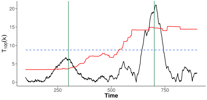
Figure 3: MOSUM detector statistic (black solid line) computed from the time series generated as described in the text with two changes in the mean (denoted by vertical lines). Also shown are the thresholds computed using global (blue dashed line) and local (red solid line) estimators of the scale-dependent TAVC.

4 Numerical results

4.1 Practical considerations

We provide guidance on the selection of tuning parameters required for the proposed robust TAVC estimator and its application with multiscale change point detection methods.

Parameter $v$ in (6).

We select $v=v_{b}=\bar{\xi}_{b}^{-1}\sqrt{G/n}$ where $\bar{\xi}_{b}$ is a fixed constant for a given $b\in\{0,\ldots,G-1\}$. For the problem of robust mean estimation, Catoni, (2012) recommends the standard deviation in the place of $\bar{\xi}_{b}$ and in a similar vein, Chen et al., (2021) propose to use a trimmed mean

$$\bar{\xi}_{[1],b}={\frac{1}{\lfloor 3N_{1}(b)/4\rfloor-\lceil N_{1}(b)/4\rceil+1}}\sum_{j=\lceil N_{1}(b)/4\rceil}^{\lfloor 3N_{1}(b)/4\rfloor}\xi_{(j),b},$$ (16)

where $\xi_{(1),b}\leq\ldots\leq\xi_{(N_{1}(b)),b}$ are the ordered $\{\xi_{j,b}\}_{j=1}^{N_{1}(b)}$. Another approach is to use an appropriately scaled median of $\{\xi_{j,b}\}_{j=1}^{N_{1}(b)}$, in a similar fashion to McGonigle et al., (2021). In this case, the necessary scaling constant to ensure unbiasedness can be chosen by noting that $\bar{X}_{j,b}$ is asymptotically Gaussian as $L\to\infty$, and thus $\xi_{j,b}$ is asymptotically scaled $\chi^{2}_{1}$. This leads to the choice

$$\bar{\xi}_{[2],b}=K\cdot\text{Median}\left\{\xi_{1,b},\ldots,\xi_{N_{1}(b),b}\right\},$$ (17)

where $K=2.125$. In simulation studies, we report the results obtained with $\bar{\xi}_{[\ell],b}$, $\ell=1,2$, in setting the parameter $v_{b}$ where we observe that both choices return similarly good results.

Parameters $b$ and $b_{\max}$ in (6).

As a further step to ensure greater robustness of the estimator, we obtain the estimator $\widehat{\sigma}^{2}_{L,b}$ for a range of $b\in\{0,\ldots,b_{\max}\}$ and take their median as the final estimator $\widehat{\sigma}^{2}_{L}$. Informally, we may get unlucky with some starting value $b$ that leads to many of the $\xi_{j,b}$ contaminated by the mean changes, and taking the median over a range of values of $b$ helps in alleviating this. We take $b_{\max}=G-1$ in practice which yields good performance.

Maximum time-scale $M$.

We recommend $M=\lfloor 2.5\sqrt{n}\rfloor$ as the coarsest scale at which the scale-dependent TAVC is estimated. This choice is made to balance between mitigating the effect of change points, and ensuring that the TAVC at coarser scales is well-approximated by $\sigma^{2}_{M}$.

Tuning parameters for the multiscale MOSUM procedure.

We follow Cho and Kirch, (2022) and generate $\mathcal{G}$ as a sequence of Fibonacci numbers. For the simulation studies reported in Section 4.2 and Appendix B, we consider $\mathcal{G}=\{G_{m},\,1\leq m\leq 4:\,G_{1}<\ldots<G_{4}\}$ where $G_{m}=G_{m-1}+G_{m-2}$ for $m\geq 2$ with $G_{0}=G_{1}=20+10\lfloor n/1000\rfloor$. For other tuning parameters, we adopt the recommended default values of the R package mosum (Meier et al.,, 2021), and set $\alpha=0.05$ and $\eta=0.4$.

Tuning parameters for the WBS2 algorithm.

For the threshold, we set the constant $C=1.3$ and draw $R=100$ deterministic intervals at each iteration, which are suggested choices in Fryzlewicz, (2014) and Cho and Fryzlewicz, (2021) respectively. As we permit the presence of serial correlations, it is reasonable to impose a minimum length requirement on the intervals considered in the WBS2 algorithm. We set this minimum length to be $2G_{1}$, with $G_{1}$ the finest scale considered by the MOSUM procedure.

Window size $W$ for time-varying TAVC estimation.

We utilise a scale-dependent window size $W_{L}$. Setting $W_{L}=N_{2}L$ gives $N_{3}=2N_{2}-1$ data points used in the solving of the $M$-estimation equations. We advise setting $N_{2}=5$, which ensures that the influence of change points is negated and that the window size is large enough to include enough data points for reliable estimation of the TAVC.

4.2 Simulation study

In this section, we evaluate the performance of the proposed robust estimator of scale-dependent TAVC applied with the two multiscale change point detection procedures discussed in Sections 3.1–3.2. We compare with other methods that account for serial dependence under (2) and whose implementations are readily available in R, with a variety of scenarios for generating serially correlated $\{\varepsilon_{t}\}_{t\in\mathbb{Z}}$.

4.2.1 Settings

We assess the performance of different methods both in the case of no changes ($q=0$) and multiple changes ($q\geq 1$), under a variety of error structures. Unless stated otherwise, we generate $W_{t}\sim_{\text{i.i.d.}}\mathcal{N}(0,\sigma_{w}^{2})$ with $\sigma_{w}=1$.

1. $\varepsilon_{t}=W_{t}$.

2. $\varepsilon_{t}=W_{t}$, where $W_{t}$ are i.i.d. $t_{5}$-distributed random variables.

3. AR(1) model: $\varepsilon_{t}=a_{1}\varepsilon_{t-1}+W_{t}$, with $a_{1}=0.9$ and $\sigma_{w}=\sqrt{1-a_{1}^{2}}$.

4. AR(2) model: $\varepsilon_{t}=a_{1}\varepsilon_{t-1}+a_{2}\varepsilon_{t-2}+W_{t}$, with $a_{1}=0.5$ and $a_{2}=0.3$, with $\sigma_{w}=0.6676184$.

5. MA(1) model: $\varepsilon_{t}=W_{t}+b_{1}W_{t-1}$, with $b_{1}=-0.9$.

6. ARCH(1) model: $\varepsilon_{t}=\sigma_{t}W_{t}$ with $\sigma_{t}^{2}=c_{0}+c_{1}\varepsilon_{t-1}^{2}$, where $c_{0}=0.5$, $c_{1}=0.4$.

7. Time-varying AR(1) model: $\varepsilon_{t}=a_{1}(t)\varepsilon_{t-1}+W_{t}$, with $a_{1}(t)=0.8-0.6t/n$.

8. Time-varying AR(1) model: $\varepsilon_{t}=a_{1}(t)\varepsilon_{t-1}+\sigma(t)W_{t}$, with $a_{1}(t)=0.5\cos(2\pi t/n)$ and $\sigma(t)=\sqrt{1-a_{1}(t)^{2}}$.

9. Time-varying MA(1) model: $\varepsilon_{t}=W_{t}+b_{1}(t)W_{t-1}$, with $b_{1}(t)=12(t/n)^{3}-18(t/n)^{2}+6t/n$.

Models (M1)–(M6) represent stationary error scenarios. Model (M1) is the setting commonly adopted in the literature while (M2), taken from Cho and Kirch, (2021), is adopted to examine whether a method works well in the presence of non-Gaussian errors. Models (M3) and (M4) allow strong autocorrelations in $\{\varepsilon_{t}\}_{t=1}^{n}$. Under Model (M5), the LRV is close to zero, which makes its accurate estimation difficult. Model (M6) is a non-linear process. Models (M7)–(M9) consider time-varying dependence structure; variants of (M7) and (M8) were studied in McGonigle et al., (2021) and Cho and Fryzlewicz, (2021), respectively. For Models (M1)–(M6), we use the global scale-dependent TAVC estimator described in Section 2.2 while for (M7)–(M9), we use the window-based estimator of the local scale-dependent TAVC described in Section 3.3.

We assess the performance of the methods both when $q=0$ and $q\geq 1$. In the latter case, the time series contains the $q$ change points at $\tau_{i}=\lfloor n/(q+1)\cdot i\rfloor,\,i=1,\ldots,q$, with the (signed) change size $\mu_{i}=\mu(\tau_{i})\cdot(-1)^{i+1}$. In (M1)–(M4) and (M6), we set $\mu(\tau_{i})=\sigma$ and in the case of (M5), we set $\mu=1$. In (M7)–(M9), we set $\mu(\tau_{i})=\sigma(\tau_{i})$ where $\sigma^{2}(t)$ denotes the time-varying LRV.

We implement the robust TAVC estimation within both the multiscale MOSUM and WBS2 procedures as described in Sections 3.1 and 3.2, which are referred to as MOSUM.TAVC_[ℓ] and WBS2.TAVC_[ℓ], respectively. Here, the subscript with $\ell=1,2$, refers to the choice of the tuning parameter $\bar{\xi}_{[\ell],b}$ involved in the parameter $v$, see (16)–(17). For the choice of the tuning parameters, we refer to Section 4.1. For illustrative purposes, we also report the results of the ‘oracle’ versions of the MOSUM and WBS2 procedures referred to as MOSUM.oracle and WBS2.oracle, respectively. These methods are implemented with the true LRV $\sigma^{2}$ ($\sigma^{2}(t)$ in the case of Models (M7)–(M9)) for standardising the detector statistics, while all other tuning parameters are kept the same.

Additionally, we consider DepSMUCE (Dette et al.,, 2020), DeCAFS (Romano et al.,, 2021) and WCM.gSa (Cho and Fryzlewicz,, 2021) for comparison. DepSMUCE extends SMUCE (Frick et al.,, 2014) to dependent data using a difference-type estimator of the LRV. Although not its primary objective, DeCAFS detects multiple change points in the mean assuming that the noise is a stationary AR($1$) process. The WCM.gSa method performs model selection on the sequence of models generated by the WBS2 algorithm, using an information criterion-based model selection strategy which assumes that $\{\varepsilon_{t}\}_{t\in\mathbb{Z}}$ follows an AR model of an arbitrary order. For DepSMUCE, we consider significance levels $\alpha\in\{0.05,0.2\}$. Other tuning parameters not mentioned here are chosen as recommended by the authors.

4.2.2 Results

Table LABEL:table:sim:results summarises the results of the comparative simulation study from $1000$ replications of time series of length $n=1000$ generated as in (M1)–(M9) with $q\in\{0,4\}$. Results for other values of $n\in\{500,2000\}$ are given in Appendix B, where we make similar observations as below.

When $q=0$, we report the proportion of falsely detecting any change point out of the $1000$ realisations (see the column ‘Size’ in Table LABEL:table:sim:results). When $q\geq 1$, we report the relative mean squared error (RMSE)

$$\sum_{t=1}^{n}(\widehat{f}_{t}-f_{t})^{2}/\sum_{t=1}^{n}(\widehat{f}^{*}_{t}-f_{t})^{2},$$

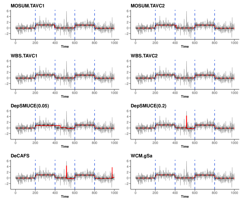
Figure 4: Comparisons of the estimator $\widehat{f}_{t}$ (red solid line) obtained from various methods in consideration and the oracle estimator $\widehat{f}^{*}_{t}$ (black dashed line) for a realisation (grey solid line) from Model (M6). True change point locations are given by blue dashed vertical lines.

where $\widehat{f}_{t}$ is the piecewise constant signal constructed with the estimated change points, and $\widehat{f}^{*}_{t}$ is the oracle estimator constructed with the true change points. For illustration, Figure 4 plots $\widehat{f}_{t}$ obtained from different methods in consideration and the oracle estimator $\widehat{f}^{*}_{t}$, on a realisation from Model (M6). We also report the distribution of the estimated number of change points, as well as the covering metric (CM). The covering metric (Arbelaez et al.,, 2010) measures the quality of the resulting segmentation as defined by the location of the detected changes, and is recommended in van den Burg and Williams, (2020) as an evaluation metric for comparing change point detection algorithms. The CM take values between $0$ and $1$, with a value of $1$ corresponding to a perfect segmentation. Its explicit definition can be found in Appendix B. For each measure, we report its average over the $1000$ realisations.

Table 1: Performance comparisons for $n=1000$. We report the size, the proportion of realisations where change points are falsely detected when $q=0$, and the distribution of the estimated number of change points, covering metric (CM) and relative MSE (RMSE) over 1000 realisations when $q=4$. The modal value of the distribution of the number of estimated change points for each method is shown in bold. The best performing method according to each metric when $q=4$ is underlined.

			$\widehat{q}-q$
Model	Method	Size	$\leq-2$	$-1$	$\mathbf{0}$	$1$	$\geq 2$	CM	RMSE
(M1)	MOSUM.TAVC[1]	0.135	0.000	0.006	0.980	0.014	0.000	0.967	6.098
	MOSUM.TAVC[2]	0.091	0.000	0.015	0.978	0.007	0.000	0.965	6.234
	WBS2.TAVC[1]	0.049	0.000	0.004	0.996	0.000	0.000	0.976	4.605
	WBS2.TAVC[2]	0.028	0.001	0.017	0.982	0.000	0.000	0.973	4.787
	DepSMUCE(0.05)	0.010	0.000	0.014	0.986	0.000	0.000	0.972	4.859
	DepSMUCE(0.2)	0.066	0.000	0.001	0.998	0.001	0.000	0.976	4.566
	DeCAFS	0.015	0.000	0.000	0.970	0.029	0.001	0.976	4.798
	WCM.gSa	0.007	0.000	0.000	0.978	0.020	0.002	0.975	4.733
	MOSUM.oracle	0.040	0.000	0.000	0.861	0.132	0.007	0.965	5.782
	WBS2.oracle	0.004	0.000	0.000	1.000	0.000	0.000	0.977	4.567
(M2)	MOSUM.TAVC[1]	0.149	0.001	0.004	0.979	0.015	0.001	0.967	6.512
	MOSUM.TAVC[2]	0.086	0.003	0.008	0.981	0.008	0.000	0.965	6.595
	WBS2.TAVC[1]	0.040	0.001	0.006	0.993	0.000	0.000	0.976	4.702
	WBS2.TAVC[2]	0.014	0.004	0.011	0.985	0.000	0.000	0.974	4.899
	DepSMUCE(0.05)	0.586	0.000	0.004	0.611	0.161	0.224	0.946	13.784
	DepSMUCE(0.2)	0.747	0.000	0.000	0.420	0.180	0.400	0.934	15.828
	DeCAFS	0.898	0.000	0.000	0.105	0.040	0.855	0.886	29.258
	WCM.gSa	0.009	0.000	0.000	0.978	0.020	0.002	0.975	4.789
	MOSUM.oracle	0.037	0.000	0.000	0.843	0.143	0.014	0.964	6.300
	WBS2.oracle	0.012	0.000	0.000	0.996	0.004	0.000	0.978	4.650
(M3)	MOSUM.TAVC[1]	0.147	0.000	0.000	0.998	0.002	0.000	0.995	1.810
	MOSUM.TAVC[2]	0.082	0.000	0.001	0.999	0.000	0.000	0.994	1.789
	WBS2.TAVC[1]	0.062	0.000	0.000	1.000	0.000	0.000	0.998	1.258
	WBS2.TAVC[2]	0.034	0.000	0.001	0.999	0.000	0.000	0.998	1.264
	DepSMUCE(0.05)	0.968	0.000	0.000	0.920	0.078	0.002	0.992	1.494
	DepSMUCE(0.2)	0.996	0.000	0.000	0.739	0.232	0.029	0.978	1.888
	DeCAFS	0.597	0.000	0.000	0.590	0.342	0.068	0.982	1.236
	WCM.gSa	0.053	0.000	0.000	0.731	0.135	0.134	0.959	2.086
	MOSUM.oracle	0.001	0.000	0.000	0.891	0.097	0.012	0.988	2.012
	WBS2.oracle	0.000	0.000	0.000	0.979	0.021	0.000	0.997	1.321
(M4)	MOSUM.TAVC[1]	0.123	0.000	0.003	0.992	0.005	0.000	0.987	3.133
	MOSUM.TAVC[2]	0.073	0.001	0.004	0.992	0.003	0.000	0.986	3.232
	WBS2.TAVC[1]	0.053	0.001	0.000	0.999	0.000	0.000	0.994	1.715
	WBS2.TAVC[2]	0.035	0.003	0.002	0.995	0.000	0.000	0.993	1.755
	DepSMUCE(0.05)	0.678	0.000	0.000	0.979	0.021	0.000	0.993	1.827
	DepSMUCE(0.2)	0.907	0.000	0.000	0.891	0.105	0.004	0.986	2.089
	DeCAFS	0.734	0.000	0.000	0.241	0.224	0.535	0.935	2.258
	WCM.gSa	0.022	0.000	0.000	0.778	0.111	0.111	0.966	2.684
	MOSUM.oracle	0.008	0.000	0.000	0.972	0.028	0.000	0.986	3.087
	WBS2.oracle	0.001	0.000	0.000	1.000	0.000	0.000	0.995	1.705
(M5)	MOSUM.TAVC[1]	0.120	0.000	0.000	1.000	0.000	0.000	0.990	89.580
	MOSUM.TAVC[2]	0.069	0.000	0.000	1.000	0.000	0.000	0.990	89.580
	WBS2.TAVC[1]	0.103	0.000	0.000	1.000	0.000	0.000	0.992	76.922
	WBS2.TAVC[2]	0.052	0.000	0.000	1.000	0.000	0.000	0.992	76.922
	DepSMUCE(0.05)	0.998	0.000	0.000	0.036	0.048	0.916	0.773	2535.266
	DepSMUCE(0.2)	1.000	0.000	0.000	0.003	0.004	0.993	0.634	1038.395
	DeCAFS	0.001	0.000	0.000	0.997	0.003	0.000	0.992	77.886
	WCM.gSa	0.000	0.000	0.000	1.000	0.000	0.000	0.992	76.814
	MOSUM.oracle	1.000	0.000	0.000	0.000	0.000	1.000	0.276	247.634
	WBS2.oracle	1.000	0.000	0.000	0.000	0.000	1.000	0.278	207.555
(M6)	MOSUM.TAVC[1]	0.168	0.000	0.000	0.978	0.021	0.001	0.973	6.246
	MOSUM.TAVC[2]	0.112	0.000	0.001	0.993	0.006	0.000	0.973	6.246
	WBS2.TAVC[1]	0.064	0.000	0.000	1.000	0.000	0.000	0.981	4.833
	WBS2.TAVC[2]	0.030	0.000	0.001	0.999	0.000	0.000	0.981	4.844
	DepSMUCE(0.05)	0.507	0.000	0.000	0.740	0.176	0.084	0.963	8.026
	DepSMUCE(0.2)	0.716	0.000	0.000	0.564	0.252	0.184	0.949	9.934
	DeCAFS	0.755	0.000	0.000	0.191	0.066	0.743	0.911	25.250
	WCM.gSa	0.021	0.000	0.000	0.971	0.018	0.011	0.978	5.406
	MOSUM.oracle	0.021	0.000	0.000	0.881	0.109	0.010	0.969	6.300
	WBS2.oracle	0.005	0.000	0.000	0.995	0.005	0.000	0.981	4.863
(M7)	MOSUM.TAVC[1]	0.247	0.000	0.002	0.970	0.025	0.003	0.973	5.232
	MOSUM.TAVC[2]	0.171	0.000	0.004	0.972	0.023	0.001	0.972	5.310
	WBS2.TAVC[1]	0.184	0.000	0.004	0.988	0.008	0.000	0.971	5.004
	WBS2.TAVC[2]	0.125	0.000	0.010	0.987	0.003	0.000	0.970	5.114
	DepSMUCE(0.05)	0.747	0.000	0.175	0.718	0.107	0.000	0.928	7.807
	DepSMUCE(0.2)	0.921	0.000	0.019	0.716	0.258	0.007	0.960	5.416
	DeCAFS	0.830	0.000	0.000	0.652	0.171	0.177	0.958	6.217
	WCM.gSa	0.471	0.059	0.041	0.830	0.044	0.026	0.941	6.975
	MOSUM.oracle	0.015	0.000	0.000	0.903	0.094	0.003	0.969	5.312
	WBS2.oracle	0.005	0.000	0.000	1.000	0.000	0.000	0.975	4.884
(M8)	MOSUM.TAVC[1]	0.244	0.000	0.001	0.947	0.052	0.000	0.969	6.884
	MOSUM.TAVC[2]	0.154	0.000	0.001	0.961	0.038	0.000	0.969	6.918
	WBS2.TAVC[1]	0.160	0.000	0.002	0.995	0.003	0.000	0.967	6.565
	WBS2.TAVC[2]	0.107	0.000	0.003	0.994	0.003	0.000	0.967	6.658
	DepSMUCE(0.05)	0.219	0.032	0.641	0.306	0.019	0.002	0.817	17.602
	DepSMUCE(0.2)	0.483	0.000	0.252	0.633	0.105	0.010	0.904	10.411
	DeCAFS	0.341	0.001	0.002	0.652	0.153	0.192	0.953	9.188
	WCM.gSa	0.173	0.076	0.159	0.748	0.011	0.006	0.913	8.976
	MOSUM.oracle	0.045	0.000	0.000	0.841	0.142	0.017	0.962	7.206
	WBS2.oracle	0.013	0.000	0.000	0.996	0.004	0.000	0.971	5.960
(M9)	MOSUM.TAVC[1]	0.311	0.000	0.008	0.915	0.076	0.001	0.963	7.027
	MOSUM.TAVC[2]	0.204	0.000	0.020	0.931	0.049	0.000	0.962	7.026
	WBS2.TAVC[1]	0.234	0.000	0.020	0.972	0.008	0.000	0.958	8.451
	WBS2.TAVC[2]	0.167	0.000	0.029	0.968	0.003	0.000	0.958	8.143
	DepSMUCE(0.05)	0.130	0.181	0.806	0.013	0.000	0.000	0.743	13.448
	DepSMUCE(0.2)	0.380	0.022	0.874	0.094	0.010	0.000	0.774	11.770
	DeCAFS	0.075	0.034	0.414	0.431	0.078	0.043	0.858	10.028
	WCM.gSa	0.054	0.057	0.695	0.236	0.009	0.003	0.814	10.822
	MOSUM.oracle	0.101	0.000	0.000	0.760	0.211	0.029	0.957	7.436
	WBS2.oracle	0.080	0.000	0.000	0.827	0.171	0.002	0.950	7.927

Overall, WBS2.TAVC displays better size control than MOSUM.TAVC. The multiscale MOSUM procedure with bottom-up merging has been noted to return false positives as it accepts all estimators from the finest bandwidth; see the simulation results reported in Cho and Kirch, (2022). Despite this known issue, MOSUM.TAVC shows better size control than some of the competitors such as DepSMUCE and DeCAFS. Between the two choices of the parameter $v$ used in (6), the one involving (17) (corresponding to the subscript $2$) yields the estimator of TAVC that returns better size control, e.g. closer to the nominal level $\alpha=0.05$ for the multiscale MOSUM procedure. On the other hand, using the trimmed mean (corresponding to the subscript $1$) as in (16) sees improved power at the cost of larger size. This suggests that an approach combining the two choices of $v$ may yield a more balanced performance.

WBS2.TAVC performs the best across all metrics and scenarios among non-oracle methods when $q\geq 1$. Also, we observe that using the proposed robust estimator of scale-dependent TAVC, compares favourably to the multiscale methods applied with the true LRV (i.e. MOSUM.oracle and WBS2.oracle) and in some scenarios, the former outperforms the respective oracle counterpart. In particular, in Scenario (M5) where the LRV is close to $0$, plugging in its true value leads to detecting many false positives. This shows that adopting the scale-dependent TAVC in place of the LRV for test statistic standardisation improves the finite sample performance when the change point detection procedure involves localised testing, as is the case for both the MOSUM and the WBS2 procedures. We make a similar observation about the performance of DepSMUCE which also sets out to estimate the LRV. DeCAFS exhibits good detection power but tends to over-estimate the number of change points as well as failing to control the size adequately even when it is applied to the correctly specified scenario (Model (M3)). WCM.gSa performs well in correctly estimating the number of change points regardless of whether $q=0$ or $q\geq 1$. However, its performance deteriorates in the presence of nonstationarities, see (M7)–(M9).

Further inspection of the results under (M9) demonstrates one advantage of the time-varying approach. Figure 5 plots the histogram of the estimated change point locations across the $1000$ replications for each of the methods. We see that the competing approaches struggle to detect the final change point due to the decreased variability towards the end of the data sequence, whereas the proposed estimator of time-varying scale-dependent TAVC successfully extends to the locally stationary scenarios.

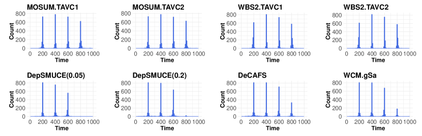
Figure 5: Histograms plotting the change point estimators returned by different methods under Model (M9).

4.3 Data applications

We apply MOSUM.TAVC and WBS2.TAVC, the multiscale procedures combined with the robust estimator of scale-dependent TAVC, to two data examples. We select the parameter $v$ in (6) using (16) and select other tuning parameters as described in Section 4.1 unless specified otherwise.

4.3.1 House price index data

We analyse the monthly percentage changes in UK house price index (HPI), which provides insight into the estimated overall changes in house prices across the UK. The data are available from https://www.gov.uk/government/statistical-data-sets/, and a detailed description of the calculation of the HPI can be found from UK Land Registry, (2021). The HPI series for various regions of the UK have previously been analysed in Baranowski et al., (2019) and McGonigle et al., (2021). We analyse the HPI for detached properties in the area of Somerset West and Taunton between April 1995 and February 2022 ($n=323$).

We set the tuning parameters as described in Section 4.1 except for the window size $W=4L$, $C=1.15$ (for WBS2.TAVC) and $\alpha=0.1$ (for MOSUM.TAVC) due to the short length of the time series. We combine the multiscale change point detection procedures with the robust estimator of the time-varying, scale-dependent TAVC described in Section 3.3, with the bandwidths $\mathcal{G}=\{20,40,60\}$ for the MOSUM procedure and the minimum interval length set at $40$ for WBS2. The data are shown in Figure 6, with the change points detected by WBS2.TAVC and MOSUM.TAVC as well as the resulting estimated mean signal given in the top and bottom panels, respectively. For comparison, we also apply DepSMUCE, DeCAFS and WCM.gSa to the data, see Table 2.

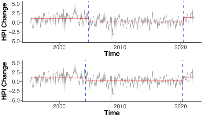
Figure 6: Monthly percentage change in HPI for detached properties in Somerset West and Taunton. Change point estimators returned by WBS2.TAVC (top) and MOSUM.TAVC (bottom) are denoted by dashed vertical lines, and the estimated means are given by solid line.

Both WBS2.TAVC and MOSUM.TAVC detect two changes. The first change, detected in May and November 2004 for the two methods, corresponds to a decrease in the mean of the HPI series. The second change, detected in May/June 2020, may be associated with the changing consumer demand for housing in the wake of the COVID-19 pandemic. The Taunton area saw the biggest increase in overall house prices in 2021, as the “race for space” saw buyers opt for “more space to work from home as well as more outdoor space” (The Guardian,, 2021).

We observe that no changes are detected by either WBS2.TAVC or MOSUM.TAVC during the 2008–2009 period associated with the financial crisis. In contrast, DepSMUCE (with $\alpha=0.2$), DeCAFS and WCM.gSa detect changes during this time period, possibly influenced by the increased variability during the financial crisis. Changes detected in the crisis period can be attributed to changes in variance (and autocorrelation), rather than those in mean, as noted in McGonigle et al., (2021). We further support this interpretation by estimating the time-varying variance after adjusting for the shifts in mean using the change point estimators returned by WBS2.TAVC, using the wavelet-based framework of Nason et al., (2000) implemented for non-dyadic data as described in McGonigle et al., (2022), see Figure 7. There is a clear period of increased variance between 2007–2010, likely due to the financial crisis. By utilising a time-varying TAVC estimator, our proposed methodology is able to capture the increased variability during this period, which ensures that potential false positives are not detected. Furthermore, by accounting for the decrease in variability towards the end of the series, our time-varying estimator of the scale-dependent TAVC allows for the detection of a change in 2020 that is missed by other methods.

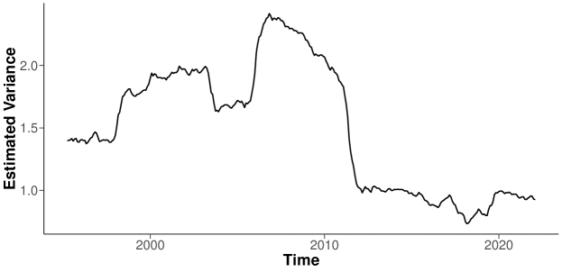
Figure 7: Estimated variance of the mean change-adjusted Somerset West and Taunton HPI series.

Table 2: Change points detected from the monthly HPI series for Somerset West and Taunton from April 1995 to February 2022.

Method	Detected change points
WBS2.TAVC	2004-11, 2020-06
MOSUM.TAVC	2004-05, 2020-05
DepSMUCE(0.05)	2004-11
DepSMUCE(0.2)	2008-09
DeCAFS	1999-05, 2003-01, 2008-08, 2009-01
WCM.gSa	1999-05, 2003-01, 2007-09, 2009-01, 2021-08

4.3.2 Nitrogen dioxide concentration in London

We analyse the daily average concentrations of nitrogen dioxide (NO₂), measured in $\mu g/m^{3}$, recorded at Marylebone Road in London, UK. The measurements were taken from January 1st, 2000 until October 31st, 2021 ($n=7734$). The data set is available from https://www.londonair.org.uk and a similar dataset was analysed for shifts in the mean in Cho and Fryzlewicz, (2021) using the WCM.gSa method. The data take positive values and display both seasonality and effects due to bank holidays, as the main source of NO₂ emissions at the site is likely to be road traffic. To mitigate these effects, we take the square root transform of the data and remove seasonality as described in Cho and Fryzlewicz, (2021).

We apply WBS2.TAVC and MOSUM.TAVC using the global TAVC estimator in (6), with the minimum interval length set at $80$ for WBS2.TAVC and the bandwidths set as $\mathcal{G}=\{40,80,120,200,320,520,840\}$ for the MOSUM.TAVC. All other tuning parameters are selected as in Section 4.1. The transformed data are shown in Figure 8, with change points detected by WBS2.TAVC and MOSUM.TAVC and the resulting estimated mean signals given in the top and bottom panels, respectively. For comparison, we also apply DepSMUCE, DeCAFS and WCM.gSa to the data. Except for DeCAFS, which detects 17 change points, all methods return similar estimators. For brevity, the DeCAFS method is omitted from the results reported in Table 3.

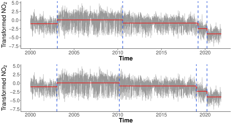
Figure 8: Transformed daily NO₂ measurements taken at Marylebone Road, London, UK. Change point estimators returned by WBS2.TAVC (top) and MOSUM.TAVC (bottom) are denoted by dashed vertical lines, and the estimated meanx are given by solid lines.

Both WBS2.TAVC and MOSUM.TAVC detect four change points, some of which can be linked to policy changes likely affecting the levels of air pollutants. In February 2003, traffic management measures were introduced in central London which included modification of the pollutant filters of London buses and other heavy duty diesel vehicles, leading to an increase in their NO₂ emissions (Air Quality Expert Group,, 2004). This corresponds to the change on January 31st, 2003 detected by all methods. Also, Marylebone Road lies within the ultra low emission zone (ULEZ) that was introduced in April 2019. The ULEZ places restrictions on the levels of pollutants of vehicles travelling in the zone, and can be linked to the change on March 10th, 2019 detected by WBS2.TAVC or earlier in 2018 by other methods considering the bias in the change point estimators. This corresponds to a decrease in the concentration of NO₂. The final change point, detected by all methods on March 18th, 2020, aligns with the nationwide lockdown due to the COVID-19 pandemic on March 23rd, 2020, which resulted in drastically reduced levels of NO₂ throughout the UK (Higham et al.,, 2021).

Table 3: Change points detected from the daily average concentrations of NO₂ at Marylebone Road in London from January 1st, 2000 to October 31st, 2021.

Method	Detected change points
WBS2.TAVC	2003-01-31, 2010-07-25, 2019-03-10, 2020-03-18
MOSUM.TAVC	2003-01-11, 2010-03-06, 2018-12-30, 2020-03-18
DepSMUCE(0.05)	2003-01-31, 2010-07-25, 2018-10-14, 2020-03-18
DepSMUCE(0.2)	2003-01-31, 2008-08-31, 2012-10-04, 2018-10-14, 2020-03-18
WCM.gSa	2003-01-31, 2009-12-09, 2018-10-14, 2020-03-18

5 Conclusions

We propose an estimator of scale-dependent TAVC that is robust to the presence of (possibly) multiple mean shifts. It is readily combined with multiscale change point detection methodologies which, by scanning for change points over data sections of varying lengths, provide good adaptivity to the problem of multiple change point detection. We show the consistency of the proposed estimator under general assumptions permitting heavy tails and serial dependence decaying at a polynomial rate, and investigate its use with the multiscale MOSUM procedure and the WBS2 algorithm. Through extensive numerical studies, we demonstrate the benefit of adopting the proposed estimator of scale-dependent TAVC for improved finite sample performance, as it better reflects the level of variability in the local data sections involved in the multiscale methods. In particular, the heuristic extension to local stationarity shows promising performance which provides a natural avenue for future research. An implementation of the methodology in the R programming language can be found at https://github.com/EuanMcGonigle/TAVC.seg.

Appendix A Algorithms and further description

A.1 Multiscale MOSUM procedure with bottom-up merging

Algorithm 1 provides a pseudocode for the multiscale MOSUM procedure with bottom-up merging combined with the robust estimation of TAVC.

Input: Data $\{X_{t}\}_{t=1}^{n}$, set $\mathcal{G}$ of bandwidths, $\alpha,\eta\in(0,1)$, maximum scale $M$ for TAVC estimation

Initialise $\mathcal{P}\leftarrow\mathcal{C}\leftarrow\emptyset$ for $G\in\mathcal{G}$ do

       if $2G\leq M$ then

             Set $\widehat{\sigma}^{2}_{2G}$ as the solution to (6) with $L=2G$

       else

             Set $\widehat{\sigma}^{2}_{2G}\leftarrow\widehat{\sigma}^{2}_{M}$ with $\widehat{\sigma}^{2}_{M}$ solving (6) with $L=M$

       end if

      

      $\mathcal{C}(G)\leftarrow$ Set of change point estimators obtained with bandwidth $G$ and critical value $D_{n}(G,\alpha)$ according to (12)

      for $\widehat{k}\in\mathcal{C}(G)$ do  Add $(\widehat{k},G)$ to $\mathcal{P}$

      

end for

for $\widehat{k}_{\circ}\in\mathcal{P}$ in increasing order with respect to $G$ do

       if $\min_{\widehat{k}\in\mathcal{C}}|\widehat{k}_{\circ}-\widehat{k}|\geq\eta G$ then Add $\widehat{k}_{\circ}$ to $\mathcal{C}$

      

end for

Output: $\mathcal{C}$

Algorithm 1 Multiscale MOSUM procedure with bottom-up merging

A.2 Wild binary segmentation 2 algorithm

Algorithm 2 provides a pseudocode for the WBS2 algorithm combined with the robust TAVC estimation.

Input: Data $\{X_{t}\}_{t=1}^{n}$, number of intervals $R$, minimum interval length $I_{\text{min}}$, threshold $D$, maximum scale $M$ for TAVC estimation

Function $\textnormal{{wbs2}}(\{X_{t}\}_{t=1}^{n},s,e,R,D,M,I_{\text{min}},\mathcal{C})$:

       if $e-s\leq I_{\text{min}}$ then Quit

      

      $\mathcal{A}_{s,e}\leftarrow\{(\ell,r)\in\mathbb{Z}^{2}:\,s\leq\ell<r\leq e\text{ and }r-\ell>1\}$

      if $|\mathcal{A}_{s,e}|\leq R$ then

             $\widetilde{R}\leftarrow|\mathcal{A}_{s,e}|$ and set $\mathcal{R}_{s,e}\leftarrow\mathcal{A}_{s,e}$

       else

            $\widetilde{R}\leftarrow R$ and draw $\widetilde{R}$ elements from $\mathcal{A}_{s,e}$ deterministically over an equispaced grid, to form $\mathcal{R}_{s,e}=\{(s_{m},e_{m}):\,1\leq m\leq\widetilde{R}\}$

       end if

      

      for $m\in\{1,\ldots,\widetilde{R}\}$ do

             if $e_{m}-s_{m}\leq M$ then

                   Set $\widehat{\sigma}^{2}_{s_{m},e_{m}}$ as the solution to (6) with $L=2\lfloor(e_{m}-s_{m})/2\rfloor$

             else

                   Set $\widehat{\sigma}^{2}_{s_{m},e_{m}}\leftarrow\widehat{\sigma}^{2}_{M}$ with $\widehat{\sigma}^{2}_{M}$ solving (6) with $L=M$

             end if

            

            Identify $(s_{\circ},k_{\circ},e_{\circ})=\operatorname*{arg\,max}_{(s_{m},k,e_{m}):\,1\leq m\leq\widetilde{R},\,s_{m}<k<e_{m}}|\mathcal{T}_{s_{m},k,e_{m}}|/\widehat{\sigma}_{s_{m},e_{m}}$

            if $|\mathcal{T}_{s_{\circ},k_{\circ},e_{\circ}}|/\widehat{\sigma}_{s_{m},e_{m}}>D$ then  Add $k_{\circ}$ to $\mathcal{C}$

            

            Perform $\textnormal{{wbs2}}(\{X_{t}\}_{t=1}^{n},s,k_{\circ},R,D,M,I_{\min},\mathcal{C})\cup\textnormal{{wbs2}}(\{X_{t}\}_{t=1}^{n},k_{\circ},e,R,D,M,I_{\min},\mathcal{C})$

       end for

      

Initialise $\mathcal{C}\leftarrow\emptyset$

$\textnormal{{wbs2}}(\{X_{t}\}_{t=1}^{n},0,n,R,D,M,I_{\min},\mathcal{C})$

Output: $\mathcal{C}$

Algorithm 2 Wild binary segmentation 2

Appendix B Additional numerical results

In this section, we provide further information on the simulation study carried out in Section 4.2 and report additional numerical results to demonstrate the performance of the proposed robust estimator of the scale-dependent TAVC.

The covering metric (CM) used to assess the quality of the segmentation produced by the detected change point is defined as follows. The true change locations $\{\tau_{i}\}_{i=1}^{q}$ define a partition $\mathcal{P}$ of the interval $\{1,2,\ldots,n\}$ into disjoint sets $\mathcal{A}_{i}$ such that $\mathcal{A}_{i}$ is the segment $\{\tau_{i-1}+1,\ldots,\tau_{i}\}$. Similarly, the estimated change locations $\{\widehat{\tau}_{i}\}_{i=1}^{\widehat{q}}$ yield a partition $\widehat{\mathcal{P}}$ of segments $\widehat{\mathcal{A}}_{i}$. Then, CM is defined by

$$C(\widehat{\mathcal{P}},\mathcal{P})=\frac{1}{n}\sum_{\mathcal{A}\in\mathcal{P}}|\mathcal{A}|\max_{\widehat{\mathcal{A}}\in\widehat{\mathcal{P}}}\left\{\frac{|\mathcal{A}\cap\widehat{\mathcal{A}}|}{|\mathcal{A}\cup\widehat{\mathcal{A}}|}\right\}.$$

The CM takes values between $0$ and $1$, with a value of $1$ corresponding to a perfect segmentation, i.e. $\mathcal{P}=\widehat{\mathcal{P}}$.

We repeat the simulations carried out in Section 4.2 with different values of $n\in\{500,2000\}$. When $n=500$, we introduce $q=3$ change points to the time series at times $\tau_{i}=\lfloor(n/4)i\rfloor,\,i=1,\ldots,3$. For $n=2000$, we have $q=6$ change points at times $\tau_{i}=\lfloor(n/7)i\rfloor,\,i=1,\ldots,6$. Lastly, $\mu_{i}$ is set analogously as in the main text. See Tables LABEL:table:sim:two–LABEL:table:sim:three for the results.

Table B.1: Performance comparisons when $n=500$. We report the size, the proportion of realisations where change points are falsely detected when $q=0$, and the distribution of the estimated number of change points, covering metric (CM) and relative MSE (RMSE) over 1000 realisations when $q=3$. The modal value of the distribution of the number of estimated change points for each method is shown in bold. The best performing method according to each metric when $q=3$ is underlined.

			$\widehat{q}-q$
Model	Method	Size	$\leq-2$	$-1$	$\mathbf{0}$	$1$	$\geq 2$	CM	RMSE
(M1)	MOSUM.TAVC[1]	0.116	0.006	0.033	0.944	0.017	0.000	0.944	7.188
	MOSUM.TAVC[2]	0.061	0.010	0.086	0.897	0.007	0.000	0.930	8.261
	WBS2.TAVC[1]	0.068	0.008	0.041	0.951	0.000	0.000	0.949	6.411
	WBS2.TAVC[2]	0.037	0.036	0.092	0.872	0.000	0.000	0.922	9.082
	DepSMUCE(0.05)	0.015	0.006	0.220	0.774	0.000	0.000	0.890	12.896
	DepSMUCE(0.2)	0.067	0.000	0.033	0.965	0.002	0.000	0.953	6.334
	DeCAFS	0.023	0.000	0.000	0.964	0.035	0.001	0.961	6.062
	WCM.gSa	0.011	0.000	0.000	0.963	0.026	0.011	0.958	6.227
	MOSUM.oracle	0.025	0.000	0.000	0.879	0.115	0.006	0.948	6.863
	WBS2.oracle	0.008	0.000	0.000	0.997	0.003	0.000	0.963	5.749
(M2)	MOSUM.TAVC[1]	0.131	0.003	0.033	0.944	0.020	0.000	0.946	7.020
	MOSUM.TAVC[2]	0.079	0.016	0.067	0.906	0.011	0.000	0.931	8.195
	WBS2.TAVC[1]	0.077	0.017	0.033	0.950	0.000	0.000	0.948	6.183
	WBS2.TAVC[2]	0.040	0.042	0.081	0.877	0.000	0.000	0.924	7.635
	DepSMUCE(0.05)	0.371	0.003	0.153	0.643	0.125	0.076	0.883	20.031
	DepSMUCE(0.2)	0.572	0.000	0.022	0.609	0.200	0.169	0.917	15.960
	DeCAFS	0.746	0.000	0.000	0.232	0.096	0.672	0.894	26.581
	WCM.gSa	0.013	0.000	0.000	0.977	0.022	0.001	0.959	6.521
	MOSUM.oracle	0.040	0.000	0.000	0.862	0.129	0.009	0.948	6.813
	WBS2.oracle	0.015	0.000	0.000	0.995	0.004	0.001	0.964	5.335
(M3)	MOSUM.TAVC[1]	0.168	0.000	0.003	0.992	0.005	0.000	0.991	2.038
	MOSUM.TAVC[2]	0.113	0.000	0.016	0.981	0.003	0.000	0.989	2.153
	WBS2.TAVC[1]	0.144	0.000	0.002	0.998	0.000	0.000	0.997	1.484
	WBS2.TAVC[2]	0.096	0.001	0.017	0.982	0.000	0.000	0.992	1.698
	DepSMUCE(0.05)	0.963	0.000	0.000	0.893	0.106	0.001	0.987	1.841
	DepSMUCE(0.2)	0.993	0.000	0.000	0.750	0.218	0.032	0.972	2.196
	DeCAFS	0.574	0.000	0.002	0.646	0.276	0.078	0.976	1.302
	WCM.gSa	0.160	0.000	0.000	0.498	0.185	0.317	0.887	3.262
	MOSUM.oracle	0.001	0.000	0.001	0.991	0.008	0.000	0.991	2.037
	WBS2.oracle	0.000	0.000	0.000	1.000	0.000	0.000	0.997	1.454
(M4)	MOSUM.TAVC[1]	0.130	0.001	0.016	0.977	0.006	0.000	0.979	3.419
	MOSUM.TAVC[2]	0.071	0.005	0.051	0.943	0.001	0.000	0.968	4.715
	WBS2.TAVC[1]	0.102	0.004	0.017	0.979	0.000	0.000	0.986	2.091
	WBS2.TAVC[2]	0.066	0.012	0.060	0.928	0.000	0.000	0.971	2.905
	DepSMUCE(0.05)	0.762	0.000	0.000	0.959	0.039	0.002	0.988	2.116
	DepSMUCE(0.2)	0.919	0.000	0.000	0.859	0.125	0.016	0.978	2.502
	DeCAFS	0.722	0.000	0.000	0.248	0.189	0.563	0.903	2.642
	WCM.gSa	0.113	0.000	0.000	0.623	0.156	0.221	0.921	3.682
	MOSUM.oracle	0.003	0.000	0.001	0.984	0.014	0.001	0.983	2.861
	WBS2.oracle	0.001	0.000	0.000	1.000	0.000	0.000	0.992	1.776
(M5)	MOSUM.TAVC[1]	0.095	0.000	0.000	0.965	0.035	0.000	0.985	78.044
	MOSUM.TAVC[2]	0.045	0.000	0.000	0.970	0.030	0.000	0.985	78.070
	WBS2.TAVC[1]	0.191	0.000	0.000	1.000	0.000	0.000	0.988	66.844
	WBS2.TAVC[2]	0.098	0.000	0.000	1.000	0.000	0.000	0.988	66.844
	DepSMUCE(0.05)	0.968	0.000	0.000	0.237	0.125	0.638	0.856	751.323
	DepSMUCE(0.2)	0.993	0.000	0.000	0.057	0.054	0.889	0.754	1319.156
	DeCAFS	0.004	0.000	0.000	0.983	0.014	0.003	0.988	84.649
	WCM.gSa	0.000	0.000	0.000	1.000	0.000	0.000	0.988	67.557
	MOSUM.oracle	1.000	0.000	0.000	0.000	0.000	1.000	0.284	250.212
	WBS2.oracle	1.000	0.000	0.000	0.000	0.000	1.000	0.289	201.271
(M6)	MOSUM.TAVC[1]	0.174	0.001	0.013	0.969	0.016	0.001	0.958	7.016
	MOSUM.TAVC[2]	0.079	0.005	0.030	0.955	0.010	0.000	0.953	7.527
	WBS2.TAVC[1]	0.105	0.007	0.017	0.975	0.001	0.000	0.963	6.226
	WBS2.TAVC[2]	0.058	0.015	0.048	0.937	0.000	0.000	0.951	7.041
	DepSMUCE(0.05)	0.389	0.000	0.075	0.802	0.097	0.026	0.930	12.034
	DepSMUCE(0.2)	0.579	0.000	0.014	0.727	0.178	0.081	0.939	11.923
	DeCAFS	0.647	0.000	0.000	0.304	0.120	0.576	0.906	24.573
	WCM.gSa	0.020	0.000	0.000	0.972	0.023	0.005	0.964	6.510
	MOSUM.oracle	0.025	0.000	0.000	0.922	0.073	0.005	0.958	7.303
	WBS2.oracle	0.006	0.000	0.000	0.993	0.006	0.001	0.969	5.939
(M7)	MOSUM.TAVC[1]	0.230	0.009	0.058	0.912	0.021	0.000	0.940	6.810
	MOSUM.TAVC[2]	0.160	0.015	0.102	0.866	0.017	0.000	0.928	7.928
	WBS2.TAVC[1]	0.205	0.017	0.087	0.871	0.024	0.001	0.918	8.715
	WBS2.TAVC[2]	0.141	0.038	0.124	0.823	0.015	0.000	0.904	10.482
	DepSMUCE(0.05)	0.335	0.002	0.325	0.620	0.050	0.003	0.868	11.388
	DepSMUCE(0.2)	0.577	0.000	0.095	0.717	0.183	0.005	0.924	7.381
	DeCAFS	0.399	0.002	0.002	0.713	0.184	0.099	0.940	6.843
	WCM.gSa	0.284	0.054	0.095	0.741	0.074	0.036	0.908	8.554
	MOSUM.oracle	0.016	0.000	0.000	0.924	0.073	0.003	0.954	5.573
	WBS2.oracle	0.006	0.000	0.000	0.997	0.003	0.000	0.957	5.822
(M8)	MOSUM.TAVC[1]	0.247	0.007	0.058	0.897	0.037	0.001	0.938	8.065
	MOSUM.TAVC[2]	0.164	0.013	0.087	0.877	0.021	0.002	0.929	8.329
	WBS2.TAVC[1]	0.195	0.016	0.058	0.898	0.028	0.000	0.922	9.555
	WBS2.TAVC[2]	0.142	0.027	0.114	0.848	0.011	0.000	0.906	10.293
	DepSMUCE(0.05)	0.180	0.063	0.712	0.213	0.012	0.000	0.748	16.963
	DepSMUCE(0.2)	0.397	0.009	0.434	0.482	0.072	0.003	0.832	12.487
	DeCAFS	0.301	0.006	0.023	0.662	0.199	0.110	0.930	9.065
	WCM.gSa	0.236	0.040	0.232	0.692	0.022	0.014	0.885	9.182
	MOSUM.oracle	0.034	0.000	0.001	0.863	0.131	0.005	0.947	6.526
	WBS2.oracle	0.014	0.000	0.000	0.989	0.011	0.000	0.949	6.549
(M9)	MOSUM.TAVC[1]	0.261	0.005	0.251	0.703	0.040	0.001	0.886	8.747
	MOSUM.TAVC[2]	0.163	0.014	0.348	0.615	0.023	0.000	0.861	9.839
	WBS2.TAVC[1]	0.178	0.010	0.329	0.633	0.028	0.000	0.855	10.803
	WBS2.TAVC[2]	0.117	0.025	0.440	0.520	0.015	0.000	0.825	11.536
	DepSMUCE(0.05)	0.121	0.058	0.924	0.017	0.001	0.000	0.709	11.780
	DepSMUCE(0.2)	0.309	0.008	0.897	0.084	0.011	0.000	0.725	11.289
	DeCAFS	0.084	0.004	0.660	0.224	0.081	0.031	0.774	11.858
	WCM.gSa	0.071	0.002	0.749	0.219	0.019	0.011	0.775	9.747
	MOSUM.oracle	0.137	0.000	0.000	0.754	0.216	0.030	0.941	7.328
	WBS2.oracle	0.150	0.000	0.000	0.768	0.228	0.004	0.917	8.366

Table B.2: Performance comparisons when $n=2000$. We report the size, the proportion of realisations where change points are falsely detected when $q=0$, and the distribution of the estimated number of change points, covering metric (CM) and relative MSE (RMSE) over 1000 realisations when $q=6$. The modal value of the distribution of the number of estimated change points for each method is shown in bold. The best performing method according to each metric when $q=6$ is underlined.

			$\widehat{q}-q$
Model	Method	Size	$\leq-2$	$-1$	$\mathbf{0}$	$1$	$\geq 2$	CM	RMSE
(M1)	MOSUM.TAVC[1]	0.126	0.000	0.000	0.983	0.017	0.000	0.975	5.979
	MOSUM.TAVC[2]	0.068	0.000	0.005	0.991	0.004	0.000	0.974	6.185
	WBS2.TAVC[1]	0.018	0.000	0.001	0.999	0.000	0.000	0.981	4.781
	WBS2.TAVC[2]	0.006	0.000	0.007	0.993	0.000	0.000	0.981	4.851
	DepSMUCE(0.05)	0.007	0.000	0.000	1.000	0.000	0.000	0.982	4.764
	DepSMUCE(0.2)	0.067	0.000	0.000	0.998	0.001	0.001	0.981	4.769
	DeCAFS	0.006	0.000	0.000	0.985	0.014	0.001	0.981	4.844
	WCM.gSa	0.005	0.000	0.000	0.964	0.014	0.022	0.979	6.087
	MOSUM.oracle	0.040	0.000	0.000	0.821	0.171	0.008	0.972	6.023
	WBS2.oracle	0.000	0.000	0.000	1.000	0.000	0.000	0.982	4.776
(M2)	MOSUM.TAVC[1]	0.143	0.000	0.000	0.996	0.004	0.000	0.975	5.940
	MOSUM.TAVC[2]	0.079	0.000	0.003	0.997	0.000	0.000	0.974	6.051
	WBS2.TAVC[1]	0.025	0.000	0.002	0.998	0.000	0.000	0.983	4.432
	WBS2.TAVC[2]	0.016	0.002	0.003	0.995	0.000	0.000	0.982	4.459
	DepSMUCE(0.05)	0.828	0.000	0.000	0.389	0.171	0.440	0.941	16.822
	DepSMUCE(0.2)	0.924	0.000	0.000	0.209	0.142	0.649	0.923	20.094
	DeCAFS	0.957	0.000	0.000	0.040	0.016	0.944	0.879	31.810
	WCM.gSa	0.005	0.000	0.000	0.961	0.014	0.025	0.980	4.686
	MOSUM.oracle	0.051	0.000	0.000	0.846	0.138	0.016	0.973	5.934
	WBS2.oracle	0.002	0.000	0.000	0.999	0.001	0.000	0.983	4.413
(M3)	MOSUM.TAVC[1]	0.122	0.000	0.000	0.996	0.004	0.000	0.995	2.050
	MOSUM.TAVC[2]	0.081	0.000	0.000	0.999	0.001	0.000	0.995	2.063
	WBS2.TAVC[1]	0.034	0.000	0.000	1.000	0.000	0.000	0.998	1.356
	WBS2.TAVC[2]	0.017	0.000	0.003	0.997	0.000	0.000	0.998	1.394
	DepSMUCE(0.05)	0.925	0.000	0.000	0.975	0.025	0.000	0.997	1.410
	DepSMUCE(0.2)	0.991	0.000	0.000	0.887	0.109	0.004	0.992	1.575
	DeCAFS	0.591	0.000	0.000	0.605	0.345	0.050	0.988	1.176
	WCM.gSa	0.007	0.000	0.000	0.643	0.150	0.207	0.959	2.336
	MOSUM.oracle	0.005	0.000	0.000	0.974	0.026	0.000	0.994	1.980
	WBS2.oracle	0.000	0.000	0.000	1.000	0.000	0.000	0.998	1.356
(M4)	MOSUM.TAVC[1]	0.092	0.000	0.000	0.992	0.008	0.000	0.990	3.017
	MOSUM.TAVC[2]	0.060	0.000	0.003	0.995	0.002	0.000	0.990	3.024
	WBS2.TAVC[1]	0.020	0.000	0.001	0.999	0.000	0.000	0.996	1.808
	WBS2.TAVC[2]	0.009	0.000	0.002	0.998	0.000	0.000	0.996	1.821
	DepSMUCE(0.05)	0.559	0.000	0.000	0.999	0.001	0.000	0.996	1.789
	DepSMUCE(0.2)	0.850	0.000	0.000	0.964	0.035	0.001	0.994	1.878
	DeCAFS	0.696	0.000	0.000	0.267	0.220	0.513	0.961	1.944
	WCM.gSa	0.013	0.000	0.000	0.723	0.113	0.164	0.967	2.803
	MOSUM.oracle	0.004	0.000	0.000	0.951	0.046	0.003	0.989	2.908
	WBS2.oracle	0.000	0.000	0.000	1.000	0.000	0.000	0.996	1.800
(M5)	MOSUM.TAVC[1]	0.133	0.00	0.000	1.000	0.000	0.000	0.993	87.796
	MOSUM.TAVC[2]	0.071	0.000	0.000	1.000	0.000	0.000	0.993	87.796
	WBS2.TAVC[1]	0.066	0.000	0.000	1.000	0.000	0.000	0.994	74.530
	WBS2.TAVC[2]	0.029	0.000	0.000	1.000	0.000	0.000	0.994	74.530
	DepSMUCE(0.05)	1.000	0.000	0.0000	0.000	0.000	1.000	0.613	2496.320
	DepSMUCE(0.2)	1.000	0.000	0.000	0.000	0.000	1.000	0.464	4116.486
	DeCAFS	0.000	0.000	0.000	0.993	0.007	0.000	0.994	77.484
	WCM.gSa	0.000	0.000	0.000	1.000	0.000	0.000	0.994	74.648
	MOSUM.oracle	1.000	0.000	0.000	0.000	0.000	1.000	0.265	222.751
	WBS2.oracle	0.978	0.000	0.000	0.000	0.000	1.000	0.265	188.806
(M6)	MOSUM.TAVC[1]	0.192	0.000	0.002	0.988	0.010	0.000	0.979	6.112
	MOSUM.TAVC[2]	0.117	0.000	0.002	0.995	0.003	0.000	0.979	6.259
	WBS2.TAVC[1]	0.054	0.000	0.001	0.999	0.000	0.000	0.985	4.641
	WBS2.TAVC[2]	0.029	0.001	0.001	0.998	0.000	0.000	0.985	4.662
	DepSMUCE(0.05)	0.767	0.000	0.000	0.549	0.232	0.219	0.960	9.668
	DepSMUCE(0.2)	0.931	0.000	0.000	0.336	0.257	0.407	0.944	11.982
	DeCAFS	0.903	0.000	0.000	0.090	0.040	0.870	0.911	28.388
	WCM.gSa	0.024	0.000	0.000	0.958	0.017	0.025	0.983	4.860
	MOSUM.oracle	0.029	0.000	0.000	0.892	0.101	0.007	0.978	6.151
	WBS2.oracle	0.006	0.000	0.000	0.997	0.002	0.001	0.985	4.631
(M7)	MOSUM.TAVC[1]	0.297	0.000	0.000	0.957	0.043	0.000	0.979	4.854
	MOSUM.TAVC[2]	0.214	0.000	0.001	0.971	0.027	0.001	0.979	4.840
	WBS2.TAVC[1]	0.178	0.000	0.000	0.992	0.008	0.000	0.979	4.959
	WBS2.TAVC[2]	0.120	0.000	0.001	0.997	0.002	0.000	0.979	4.984
	DepSMUCE(0.05)	0.445	0.004	0.292	0.616	0.088	0.000	0.917	9.351
	DepSMUCE(0.2)	0.726	0.000	0.035	0.670	0.284	0.011	0.963	5.326
	DeCAFS	0.557	0.000	0.000	0.492	0.216	0.292	0.961	6.242
	WCM.gSa	0.316	0.031	0.027	0.895	0.026	0.021	0.968	4.840
	MOSUM.oracle	0.036	0.000	0.000	0.878	0.111	0.011	0.975	4.933
	WBS2.oracle	0.005	0.000	0.000	0.997	0.003	0.000	0.983	4.154
(M8)	MOSUM.TAVC[1]	0.304	0.000	0.000	0.939	0.058	0.003	0.976	5.985
	MOSUM.TAVC[2]	0.195	0.000	0.000	0.960	0.039	0.001	0.976	5.934
	WBS2.TAVC[1]	0.142	0.000	0.000	0.994	0.006	0.000	0.976	5.958
	WBS2.TAVC[2]	0.081	0.000	0.001	0.998	0.001	0.000	0.977	5.796
	DepSMUCE(0.05)	0.277	0.077	0.704	0.210	0.009	0.000	0.833	15.628
	DepSMUCE(0.2)	0.595	0.004	0.361	0.514	0.113	0.008	0.901	10.853
	DeCAFS	0.368	0.000	0.000	0.594	0.199	0.207	0.965	7.261
	WCM.gSa	0.136	0.040	0.051	0.894	0.010	0.005	0.962	5.811
	MOSUM.oracle	0.060	0.000	0.000	0.805	0.174	0.021	0.971	6.190
	WBS2.oracle	0.004	0.000	0.000	0.997	0.003	0.000	0.980	5.162
(M9)	MOSUM.TAVC[1]	0.382	0.000	0.003	0.922	0.072	0.003	0.974	6.551
	MOSUM.TAVC[2]	0.259	0.000	0.004	0.953	0.042	0.001	0.974	6.549
	WBS2.TAVC[1]	0.231	0.000	0.005	0.985	0.010	0.000	0.973	7.309
	WBS2.TAVC[2]	0.181	0.000	0.003	0.993	0.004	0.000	0.974	7.153
	DepSMUCE(0.05)	0.231	0.741	0.251	0.008	0.000	0.000	0.731	13.329
	DepSMUCE(0.2)	0.540	0.269	0.616	0.106	0.008	0.001	0.784	13.165
	DeCAFS	0.081	0.262	0.022	0.574	0.092	0.050	0.890	8.834
	WCM.gSa	0.061	0.281	0.076	0.624	0.014	0.005	0.890	8.122
	MOSUM.oracle	0.097	0.000	0.000	0.754	0.215	0.031	0.968	6.883
	WBS2.oracle	0.067	0.000	0.000	0.957	0.042	0.001	0.967	6.774

Appendix C Proof of Theorem 1

For sequences of positive numbers $\{a_{n}\}$ and $\{b_{n}\}$, we write $a_{n}\lesssim b_{n}$, or $a_{n}=\mathcal{O}(b_{n})$, if there exists some constant $C>0$ such that $a_{n}/b_{n}\leq C$ as $n\to\infty$. We write $a_{n}\asymp b_{n}$ if there exists some positive constants $C_{1}$ and $C_{2}$ such that $C_{1}\leq a_{n}/b_{n}\leq C_{2}$ as $n\to\infty$. Without loss of generality, we set $b=0$ and drop the dependence on $b$ for notational simplicity; analogous arguments are applicable when other fixed values of $b\in\{0,\ldots,G-1\}$ are used.

We denote by $\mathcal{B}_{j}=\{t\in\{1,\ldots,n\}:\,jG+1\leq t\leq(j+1)G\}$ the set of indices of the $j$-th block of data for some $j=0,\ldots,\lfloor n/G\rfloor-1$. We adapt the proof of Theorem 5 in Chen et al., (2021) with modifications to our case with the TAVC estimator. We denote by

$$\mathcal{S}=\{0\leq j\leq\lfloor n/G\rfloor-1:\,\mathcal{B}_{j}\text{ or }\mathcal{B}_{j-1}\text{ contains change points}\}.$$

Then, $|\mathcal{S}|\leq 2q$. First, we consider the influence function constructed using the blocks which do not contain any change points:

$$\bar{h}_{L}(u)=\frac{1}{N_{0}}\sum_{j\notin\mathcal{S}}\phi_{v}(\xi_{j}-u)=0,\text{ where }N_{0}=N_{1}-|\mathcal{S}|.$$

Letting

$$\tilde{\xi}=\frac{1}{N_{0}}\sum_{j\notin\mathcal{S}}\mathbb{E}(\xi_{j})={\widetilde{\sigma}_{L}^{2}},\text{ and }\gamma^{2}=\frac{1}{N_{0}}\sum_{j\notin\mathcal{S}}\mathbb{E}(\xi_{j}^{2})-\tilde{\xi}^{2},$$

define the functions

$$B^{+}(u,x) =\tilde{\xi}-u+\frac{v}{2}\left[\left(\tilde{\xi}-u\right)^{2}+\gamma^{2}\right]+x,$$

$$B^{-}(u,x) =\tilde{\xi}-u-\frac{v}{2}\left[\left(\tilde{\xi}-u\right)^{2}+\gamma^{2}\right]-x.$$

Then, it can be shown that $\mathbb{E}(\bar{h}_{L}(u))$ satisfies the envelope property

$$B^{-}(u,0)\leq\mathbb{E}\left(\bar{h}_{L}(u)\right)\leq B^{+}(u,0).$$ (C.1)

To see this, note that since $\phi(x)\leq x+x^{2}/2$ by Equation (5), we have

$$\mathbb{E}\left(\bar{h}_{L}(u)\right) \leq\frac{1}{vN_{0}}\sum_{j\notin\mathcal{S}}\left[\mathbb{E}(v({\xi}_{j}-u))+\frac{1}{2}\mathbb{E}(v^{2}({\xi}_{j}-u)^{2})\right]$$

$$=\frac{1}{N_{0}}\sum_{j\notin\mathcal{S}}\mathbb{E}(\xi_{j})-u+\frac{v}{2N_{0}}\sum_{j\notin\mathcal{S}}\mathbb{E}((\xi_{j}-u)^{2})$$

$$=\tilde{\xi}-u+\frac{v}{2}\left[(\tilde{\xi}-u)^{2}+\gamma^{2}\right]=B^{+}(u,0).$$

Similarly, from the fact that $\phi(x)\geq x-x^{2}/2$, the lower bound follows.

Next, we show that $\bar{h}_{L}(u)$ is concentrated about its mean. We deal with the different cases, Assumptions 1 (iii) (iii)(a) and (iii)(b), separately, in order to prove Equations (7) and (8) respectively. Applying Step 2 of the proof of Theorem 5 in Chen et al., (2021), we have that, for $C_{0}>0$ and $x>0$,

$$\mathsf{P}\left(\sup_{u:\,|u-\widetilde{\sigma}_{L}^{2}|\leq C_{0}}\left|\bar{h}_{L}(u)-\mathbb{E}(\bar{h}_{L}(u))\right|\geq x/N_{0}\right)\leq\mathsf{P}\left(\max_{u\in A_{n}}\left|\bar{h}_{L}(u)-\mathbb{E}(\bar{h}_{L}(u))\right|\geq x/(2N_{0})\right),$$ (C.2)

where $A_{n}$ is the $\delta$-net for $\{u:|u-\widetilde{\sigma}^{2}_{L}|\leq C_{0}\}$ with $\delta=\widetilde{\sigma}^{2}_{L}x/(2N_{0})$ and $|A_{n}|=\mathcal{O}(N_{0}/x)$. For any random variable $X$, denote by $\mathbb{E}_{0}(X)=X-\mathbb{E}(X)$ the centering operator, and let $\Delta\bar{X}_{j}=\bar{X}_{j}-\bar{X}_{j-1}$. Let $\mathcal{F}_{k}=\{\eta_{t},\,t\in\cup_{l\leq k}\mathcal{B}_{l}\}$, and $\mathcal{F}_{k,\{m\}}$, $m\leq k$, be $\mathcal{F}_{k}$ with $\eta_{t}$ therein replaced with its independent and identically distributed copy $\eta^{\prime}_{t}$ for all $t\in\mathcal{B}_{m}$. Then for any random variable $X=h(\mathcal{F}_{k})$ with measurable $h(\cdot)$, let $X_{\{m\}}=h(\mathcal{F}_{k,\{m\}})$.

Proof of (7).

Under Assumption 1 (iii) (iii)(a), we show that $\zeta_{j}(u)=\phi_{v}(\xi_{j}-u)$ satisfies appropriate functional dependence properties. Denote

$$\delta_{\ell,r/2}=\max_{j\notin\mathcal{S}}\left\|\sup_{u}|\zeta_{j}(u)-\zeta_{j,\{j-\ell\}}(u)|\right\|_{r/2}.$$

Since $|\phi^{\prime}|_{\infty}\leq 1$, we have for any $\ell\in\mathbb{N}$ and $u\in\mathbb{R}$,

$$\left\|\ \sup_{u}\left|\zeta_{j}(u)-\zeta_{j,\{j-\ell\}}(u)\right|\right\|_{r/2}\leq\left\|\xi_{j}-\xi_{j,\{j-\ell\}}\right\|_{r/2}=\frac{G}{2}\|\Delta\bar{X}_{j}^{2}-\Delta\bar{X}_{j,\{j-\ell\}}^{2}\|_{r/2}$$

$$\leq\frac{G}{2}\left(\left\|\mathbb{E}_{0}\left[\Delta\bar{X}_{j}(\Delta\bar{X}_{j}-\Delta\bar{X}_{j,\{j-\ell\}})\right]\right\|_{r/2}+\left\|\mathbb{E}_{0}\left[\Delta\bar{X}_{j,\{j-\ell\}}(\Delta\bar{X}_{j}-\Delta\bar{X}_{j,\{j-\ell\}})\right]\right\|_{r/2}\right)$$

$$=\frac{G}{2}\left(I_{1}+I_{2}\right).$$ (C.3)

Further, let $E_{j,k}=\sum_{t=jG+1}^{(j+1)G}a_{t-k}$ and $U_{j}=G^{-1}\sum_{t=jG+1}^{(j+1)G}\varepsilon_{t}$. Then,

$$U_{j}=\frac{1}{G}\sum_{t=jG+1}^{(j+1)G}\sum_{k=0}^{\infty}a_{k}\eta_{t-k}=\frac{1}{G}\sum_{t=jG+1}^{(j+1)G}\sum_{k=-\infty}^{t}a_{t-k}\eta_{k}=\frac{1}{G}\sum_{k\leq(j+1)G}E_{j,k}\eta_{k},$$

and we define

$$\Delta U_{j}=\frac{1}{G}\sum_{k\leq(j+1)G}E_{j,k}\eta_{k}-\frac{1}{G}\sum_{k\leq jG}E_{j-1,k}\eta_{k}.$$

Noting that

$$G\Delta U_{j,\{j-\ell\}}=\left\{\begin{array}[]{ll}\displaystyle{\sum_{\begin{subarray}{c}k\leq(j+1)G,\\ k\notin\mathcal{B}_{j-\ell}\end{subarray}}E_{j,k}\eta_{k}+\sum_{k\in\mathcal{B}_{j-\ell}}E_{j,k}\eta_{k}^{\prime}-\sum_{\begin{subarray}{c}k\leq jG,\\ k\notin\mathcal{B}_{j-\ell}\end{subarray}}E_{j-1,k}\eta_{k}-\sum_{k\in\mathcal{B}_{j-\ell}}E_{j-1,k}\eta_{k}^{\prime}}&\text{ for }\ell\geq 1,\\ \displaystyle{\sum_{k\leq jG}E_{j,k}\eta_{k}+\sum_{k\in\mathcal{B}_{j}}E_{j,k}\eta_{k}^{\prime}-\sum_{k\leq jG}E_{j-1,k}\eta_{k}}&\text{ for }\ell=0,\end{array}\right.$$

it follows that

$$G\left(\Delta U_{j}-\Delta U_{j,\{j-\ell\}}\right)=\left\{\begin{array}[]{ll}\displaystyle{\sum_{k\in\mathcal{B}_{j-\ell}}}(E_{j,k}-E_{j-1,k})(\eta_{k}-\eta^{\prime}_{k})&\text{ for }\ell\geq 1,\\ \displaystyle{\sum_{k\in\mathcal{B}_{j}}}E_{j,k}(\eta_{k}-\eta^{\prime}_{k})&\text{ for }\ell=0.\end{array}\right.$$

Next, by Assumption 1 (i), we have

$$\left|\sum_{k\geq\ell}a_{k}\right|\leq\sum_{k\geq\ell}|a_{k}|\leq\Xi\sum_{k\geq\ell}(1+k)^{-\beta}\lesssim(1+\ell)^{-\beta+1+\epsilon}$$ (C.4)

for any arbitrarily small $\epsilon>0$. Then, using (C.4),

$$\sum_{k\in\mathcal{B}_{j-\ell}}E_{j-1,k}^{2} =\sum_{k=(j-\ell)G+1}^{(j-\ell+1)G}\left(\sum_{t=(j-1)G+1}^{jG}a_{t-k}\right)^{2}$$

$$\lesssim\sum_{k=(j-\ell)G+1}^{(j-\ell+1)G}\left((j-1)G+1-k\right)^{-2(\beta-1-\epsilon)}\lesssim G(G(\ell-1)\vee 1)^{-2(\beta-1-\epsilon)},$$ (C.5)

$$\sum_{k\leq(j+1)G}E_{j,k}^{2} =\sum_{k\leq(j+1)G}\left(\sum_{t=jG+1}^{(j+1)G}a_{t-k}\right)^{2}\lesssim\sum_{k\leq(j+1)G}\left(1\vee(jG+1-k)\right)^{-2(\beta-1-\epsilon)}\lesssim G,$$ (C.6)

where the constants involved in $\lesssim$ depend on $\epsilon$, $\beta$ and $\Xi$. Since we only consider $j\notin\mathcal{S}$, we bound $I_{1}$ in (C.3) for $\ell\geq 1$ as

$$I_{1} =\left\|\mathbb{E}_{0}\left[\Delta U_{j}(\Delta U_{j}-\Delta U_{j,\{j-\ell\}})\right]\right\|_{r/2}$$

$$=G^{-2}\left\|\mathbb{E}_{0}\left[\left(\sum_{k\leq(j+1)G}E_{j,k}\eta_{k}-\sum_{k\leq jG}E_{j-1,k}\eta_{k}\right)\left(\sum_{k\in\mathcal{B}_{j-\ell}}(E_{j,k}-E_{j-1,k})(\eta_{k}-\eta^{\prime}_{k})\right)\right]\right\|_{r/2}$$

$$\lesssim G^{-2}\left\|\sum_{k\leq(j+1)G}E_{j,k}\eta_{k}-\sum_{k\leq jG}E_{j-1,k}\eta_{k}\right\|_{r}\left\|\sum_{k\in\mathcal{B}_{j-\ell}}(E_{j,k}-E_{j-1,k})(\eta_{k}-\eta^{\prime}_{k})\right\|_{r}$$

$$\lesssim G^{-2}C_{r}^{2}\left(\sum_{k\leq(j+1)G}E_{j,k}^{2}\mu_{r}^{2}+\sum_{k\leq jG}E_{j-1,k}^{2}\mu_{r}^{2}\right)^{1/2}\left(\sum_{k\in\mathcal{B}_{j-\ell}}(E_{j,k}-E_{j-1,k})^{2}\mu_{r}^{2}\right)^{1/2}$$

$$\lesssim G^{-1}C_{r}^{2}\left(G(\ell-1)\vee 1\right)^{-(\beta-1-\epsilon)}\mu_{r}^{2},$$

where the first inequality follows from Hölder’s inequality, the second from Burkholder’s inequality (see e.g. Lemma 2 of Chen et al., (2021)) with $C_{r}=\max(\sqrt{r-1},1/(r-1))$, the last from (C.5)–(C.6) and $\mu_{r}=\|\eta_{1}\|_{r}$. Similarly, when $\ell=0$, we have that $I_{1}\lesssim G^{-1}C_{r}^{2}\mu_{r}^{2}$. We can bound the term $I_{2}$ in (C.3) in a similar fashion, to obtain

$$\delta_{\ell,r/2}\lesssim\left((G\ell)^{-(\beta-1-\epsilon)}\mathbb{I}(\ell>1)+\mathbb{I}(\ell\leq 1)\right)C_{r}^{2}\mu_{r}^{2}.$$ (C.7)

Therefore, the dependence-adjusted norm

$$w_{r/2,\alpha}=\sup_{k\geq 0}\ (k+1)^{\alpha}\sum_{\ell=k}^{\infty}\delta_{\ell,r/2}\lesssim\sup_{k\geq 2}\ (k+1)^{\alpha}\sum_{\ell=k}^{\infty}(G\ell)^{-(\beta-1-\epsilon)}C_{r}^{2}\mu_{r}^{2}\lesssim C_{r}^{2}\mu_{r}^{2},$$

for $\alpha=\beta-2-2\epsilon>1/2-2/r$ with $\beta>2.5$. Under Assumption 1 (iii) (iii)(a), having shown the bound on $w_{r/2,\alpha}$, we apply Lemma C.2 of Zhang and Wu, (2017) and yield, for any $u\in A_{n}$,

$$\mathsf{P}\left(\left|\bar{h}_{L}(u)-\mathbb{E}(\bar{h}_{L}(u))\right|\geq\frac{x}{2N_{0}}\right)\lesssim N_{0}x^{-r/2}+\exp\left(-\frac{x^{2}}{cN_{0}}\right),$$

where $c$ and the constant appearing in the $\lesssim$ depend on $r$, $\mu_{r}$, $\Xi$, $\beta$ and $\epsilon$. Applying a Bonferroni bound with $|A_{n}|=\mathcal{O}(N_{0}/x)$ then yields

$$\mathsf{P}\left(\max_{u\in A_{n}}\left|\bar{h}_{L}(u)-\mathbb{E}(\bar{h}_{L}(u))\right|\geq\frac{x}{2N_{0}}\right)\lesssim\frac{N_{0}}{x}\left(N_{0}x^{-r/2}+\exp\left(-\frac{x^{2}}{cN_{0}}\right)\right).$$ (C.8)

Taking $x\asymp N_{0}^{\frac{4}{r+2}}\vee(N_{0}\log(N_{0}))^{1/2}$, using Equations (C.2) and (C.8) we obtain

$$\sup_{|u-\widetilde{\sigma}_{L}^{2}|\leq C_{0}}\left|\bar{h}_{L}(u)-\mathbb{E}(\bar{h}_{L}(u))\right|=\mathcal{O}_{P}\left(N_{0}^{-\frac{r-2}{r+2}}\vee\sqrt{\frac{\log(N_{0})}{N_{0}}}\right).$$ (C.9)

Recalling that $|\mathcal{S}|\leq 2q$ and $|\phi(x)|\leq\log(2)$, we have that

$$\left|\frac{N_{1}h_{L}(u)}{N_{0}}-\bar{h}_{L}(u)\right|\leq\frac{2q\log(2)}{vN_{0}}.$$ (C.10)

Combining Equations (C.1), (C.9) and (C.10), we have that with probability tending to one,

$$B^{-}(u,\Delta)\leq\frac{N_{1}h_{L}(u)}{N_{0}}\leq B^{+}(u,\Delta)$$ (C.11)

uniformly for all $|u-\widetilde{\sigma}^{2}_{L}|\leq C_{0}$, where

$$\Delta=\frac{x}{N_{0}}+\frac{2q\log(2)}{vN_{0}},$$

with $x\asymp N_{0}^{\frac{4}{r+2}}\vee(N_{0}\log(N_{0}))^{1/2}$. If

$$v^{2}\gamma^{2}+2v\Delta\leq 1,$$ (C.12)

then $B^{+}(u,\Delta)$ possesses real roots. Denote the smallest root by $u^{+}$, which satisfies

$$u^{+}\leq\tilde{\xi}+\frac{\gamma^{2}+2\Delta/v}{\sqrt{1/v^{2}}}\leq\tilde{\xi}+v\gamma^{2}+2\Delta.$$ (C.13)

Under Assumption 1, we have for some $j\notin\mathcal{S}$,

$$\gamma^{2} \leq\mathbb{E}(\xi_{j}^{2})=\frac{G^{2}}{4}\mathbb{E}(\Delta\bar{X}_{j}^{4})=\frac{G^{2}}{4}\mathbb{E}(\Delta U_{j}^{4})\lesssim\frac{1}{G^{2}}\left(\left\|\sum_{k\leq(j+1)G}E_{j,k}\eta_{k}\right\|_{4}^{4}+\left\|\sum_{k\leq jG}E_{j-1,k}\eta_{k}\right\|_{4}^{4}\right)$$

$$\lesssim\frac{1}{G^{2}}\left(\sum_{k\leq(j+1)G}E_{j,k}^{2}+\sum_{k\leq jG}E_{j-1,k}^{2}\right)^{2}\mu_{4}^{4}=\mathcal{O}(1)$$

by (C.6) and Burkholder’s inequality. Therefore, from (C.13) and that $u^{+}\geq\widetilde{\xi}=\widetilde{\sigma}_{L}^{2}$,

$$u^{+}-\widetilde{\sigma}_{L}^{2}=\mathcal{O}\left(v+\frac{x}{N_{0}}+\frac{q}{vN_{0}}\right)=\mathcal{O}\left(v+\frac{Gx}{n}+\frac{Gq}{vn}\right).$$

A similar bound can be obtained for $u^{-}$, the largest root of $B^{-1}(u,\Delta)$ and under Equation (C.11), we have that $u^{-}\leq\widehat{\sigma}^{2}_{L}\leq u^{+}$. Then, setting $v\asymp(Gq/n)^{1/2}$, we have (C.12) holds, and

$$\left|\widehat{\sigma}^{2}_{L}-\widetilde{\sigma}_{L}^{2}\right|=\mathcal{O}_{P}\left(\sqrt{\frac{Gq}{n}}+\max\left\{\left(\frac{G}{n}\right)^{\frac{r-2}{r+2}},\sqrt{\frac{G\log(n)}{n}}\right\}\right).$$

∎

Proof of (8).

We proceed analogously as in the proof of (7), except that we control for the dependence-adjusted sub-exponential norm of $\zeta_{j}(u)$, as

$$\tilde{w}_{f}=\sup_{r\geq 2}r^{-f}\sum_{\ell=0}^{\infty}\delta_{\ell,r}\lesssim\ \sup_{r\geq 2}r^{-f}\sum_{\ell=0}^{\infty}\left((G\ell)^{-(\beta-1-\epsilon)}\mathbb{I}(\ell>1)+\mathbb{I}(\ell\leq 1)\right)C_{2r}^{2}\mu_{2r}^{2}\lesssim\sup_{r\geq 2}r^{-f+2\kappa+1},$$

where the first inequality follows from (C.7) and the second from Assumption 1 (i). Therefore, we have $\tilde{w}_{f}<\infty$ with $f=2\kappa+1$. Then applying Lemma C.4 of Zhang and Wu, (2017) with (C.2), we obtain

$$\mathsf{P}\left(\sup_{|u-\widetilde{\sigma}_{L}^{2}|\leq C_{0}}\left|\bar{h}_{L}(u)-\mathbb{E}(\bar{h}_{L}(u))\right|\geq\frac{x}{N_{0}}\right)\lesssim\frac{N_{0}}{x}\exp\left(-\frac{(x/\sqrt{N_{0}})^{\frac{2}{4\kappa+3}}}{c}\right),$$

where $c$ depends on $\kappa$ and $\beta$ through $\tilde{w}_{f}$. Taking $x\asymp\log^{2\kappa+3/2}(n)N_{0}^{1/2}$, we have that

$$\sup_{|u-\widetilde{\sigma}_{L}^{2}|\leq C_{0}}\left|\bar{h}_{L}(u)-\mathbb{E}(\bar{h}_{L}(u))\right|=\mathcal{O}_{P}\left(\frac{\log^{2\kappa+3/2}(n)}{\sqrt{N_{0}}}\right).$$ (C.14)

Then, by the analogous arguments as those adopted in the proof of (7) with (C.14) replacing (C.9), we derive (8). ∎

Proof of (9).

Recalling that $U_{j}=G^{-1}\sum_{t=jG+1}^{(j+1)G}\varepsilon_{t}$, we have

$$\widetilde{\sigma}^{2}_{L}=\frac{G}{2}\mathbb{E}\left((U_{j}-U_{j-1})^{2}\right) =\frac{G}{2}\mathbb{E}(U_{j}^{2}+U_{j-1}^{2}-2U_{j}U_{j-1})=\sigma^{2}_{G}-G\mathbb{E}(U_{j}U_{j-1}),$$

while

$${\sigma}^{2}_{L} =\mathbb{E}\left(\left(\frac{1}{\sqrt{L}}\sum_{t=1}^{L}\varepsilon_{t}\right)^{2}\right)=\mathbb{E}\left(\left(\frac{1}{\sqrt{L}}\sum_{t=1}^{G}\varepsilon_{t}+\frac{1}{\sqrt{L}}\sum_{t=G+1}^{L}\varepsilon_{t}\right)^{2}\right)$$

$$=\frac{1}{2}(\sigma^{2}_{G}+\sigma^{2}_{G})+\frac{2}{L}\mathbb{E}\left(\sum_{t=1}^{G}\varepsilon_{t}\sum_{t^{\prime}=G+1}^{L}\varepsilon_{t^{\prime}}\right)=\sigma^{2}_{G}+G\mathbb{E}(U_{j}U_{j-1}).$$

By Assumption 1 (i), $\rho_{k}=\mathbb{E}(\varepsilon_{0}\varepsilon_{k})$, $k\geq 0$, satisfy

$$|\rho_{k}|=\left|\sum_{j=0}a_{j}a_{j+k}\right|\leq\sum_{j=0}^{\infty}|a_{j}a_{j+k}|\lesssim\sum_{j=0}^{\infty}(j+1)^{-\beta}(j+k+1)^{-\beta}\leq k^{-\beta}\sum_{j=0}^{\infty}(j+1)^{-\beta}=\mathcal{O}(k^{-\beta}).$$

Therefore,

$$|\widetilde{\sigma}^{2}_{L}-\sigma_{L}^{2}| =L|\mathbb{E}(U_{j}U_{j-1})|=\frac{4}{L}\sum_{t=1}^{G}\sum_{t^{\prime}=G+1}^{L}\mathbb{E}(\varepsilon_{t}\varepsilon_{t^{\prime}})=\frac{4}{L}\left(\sum_{k=1}^{G}k\rho_{k}+\sum_{k=1}^{G-1}(G-k)\rho_{k+G}\right)$$

$$\lesssim L^{-1}\left(\sum_{k=1}^{G}k^{1-\beta}+\sum_{k=1}^{G-1}(G-k)(k+G)^{-\beta}\right)\lesssim L^{-1}\left(1+L^{2-\beta}\right)=\mathcal{O}\left(L^{-1}\right).$$

Lastly, to prove the second statement in Equation (10), we show that

$$|\sigma^{2}_{L}-\sigma^{2}|\leq\left|\sum_{k:\,|k|\geq L}\rho_{k}\right|+L^{-1}\left|\sum_{k=-L+1}^{L-1}|k|\rho_{k}\right|=\mathcal{O}(L^{-\beta+1}+L^{-1})=\mathcal{O}(L^{-1}),$$

which completes the proof. ∎

References

- Air Quality Expert Group, (2004) Air Quality Expert Group (2004). Nitrogen dioxide in the United Kingdom. https://uk-air.defra.gov.uk/library/assets/documents/reports/aqeg/nd-chapter2.pdf. Accessed 01/03/2022.
- Arbelaez et al., (2010) Arbelaez, P., Maire, M., Fowlkes, C., and Malik, J. (2010). Contour detection and hierarchical image segmentation. IEEE Transactions on Pattern Analysis and Machine Intelligence, 33(5):898–916.
- Aue and Horváth, (2013) Aue, A. and Horváth, L. (2013). Structural breaks in time series. Journal of Time Series Analysis, 34:1–16.
- Baranowski et al., (2019) Baranowski, R., Chen, Y., and Fryzlewicz, P. (2019). Narrowest-over-threshold detection of multiple change points and change-point-like features. Journal of the Royal Statistical Society: Series B (Statistical Methodology), 81(3):649–672.
- Catoni, (2012) Catoni, O. (2012). Challenging the empirical mean and empirical variance: A deviation study. Annales de l’Institut Henri Poincaré, Probabilités et Statistiques, 48(4):1148–1185.
- Chakar et al., (2017) Chakar, S., Lebarbier, E., Lévy-Leduc, C., and Robin, S. (2017). A robust approach for estimating change-points in the mean of an AR(1) process. Bernoulli, 23(2):1408–1447.
- Chan, (2022) Chan, K. W. (2022). Optimal difference-based variance estimators in time series: A general framework. The Annals of Statistics, 50(3):1376–1400.
- Chen et al., (2021) Chen, L., Wang, W., and Wu, W. B. (2021). Inference of breakpoints in high-dimensional time series. Journal of the American Statistical Association, pages 1–13.
- Cho and Fryzlewicz, (2021) Cho, H. and Fryzlewicz, P. (2021). Multiple change point detection under serial dependence: Wild contrast maximisation and gappy Schwarz algorithm. arXiv preprint arXiv:2011.13884.
- Cho and Kirch, (2021) Cho, H. and Kirch, C. (2021). Data segmentation algorithms: Univariate mean change and beyond. Econometrics and Statistics (to appear).
- Cho and Kirch, (2022) Cho, H. and Kirch, C. (2022). Two-stage data segmentation permitting multiscale change points, heavy tails and dependence. Annals of the Institute of Statistical Mathematics, 74(4):653–684.
- Chu et al., (1995) Chu, C.-S. J., Hornik, K., and Kaun, C.-M. (1995). MOSUM tests for parameter constancy. Biometrika, 82(3):603–617.
- Dette et al., (2020) Dette, H., Eckle, T., and Vetter, M. (2020). Multiscale change point detection for dependent data. Scandinavian Journal of Statistics, 47(4):1243–1274.