New description of neutrino flavour evolution in solar matter

Abstract

Assuming that the interacting neutrino and the solar matter can be treated as an open quantum system we formulate a formalism of neutrino state evolution in terms of the Bloch vector, obtained by solving a quasilinear extension of the von Neumann equation. We broaden the classical Wolfenstein formalism by means of exploiting the strictly linear von Neumann equation and reinterpreting the results in terms of the quantities appropriate for the quasilinear approach. We obtain similar predictions for the averaged neutrino survival probability measured on Earth in both approaches, differing by details inside the Sun where the quasilinear evolution predicts a suppression of oscillations. We discuss the issues of energy transfer between the neutrino and the Sun and the speed of the state evolution in both approaches.

1 Introduction

The fact that the pattern of neutrino oscillations in matter deviates from that in the vacuum was recognised and mathematically described by Wolfenstein more than 40 years ago. His formalism was based on an assumption of a linear evolution of the neutrino state, involving a free Hamiltonian and the so-called Wolfenstein potential (proportional to the electron number density) as the interaction term cite:Wolfenstein78 ; cite:Wolfenstein79 . In the 80-ties this topic was expanded by Mikheev and Smirnov who also reestablished a new nomenclature, such as "resonance enhancement of oscillations" and "adiabatic flavour conversion", as well as emphasised the role of effective flavour mixing (mentioned already by Wolfenstein), induced by the varying Wolfenstein potential in the course of neutrino evolution in the solar matter cite:MS1 ; cite:MS2 ; cite:MS3 ; cite:MS4 ; cite:MSW1 . The MSW effect, linked to this formalism, explained the deficit of $\nu_{e}$’s in the solar flux measured on Earth, compared to predictions of the Standard Solar Model, and also allowed to calculate corrections to neutrino oscillations in the terrestrial matter. We now note that one circumstance should be taken into account in developing an appropriate evolution formalism. Namely, in reality the propagating neutrino interacts with the solar plasma, rather not with a potential field, in a way understood for an open system, i.e., subsystem (neutrino) and environment (plasma), respectively. Thus we can expect that a complete description of the neutrino flavour state can be obtained by solving an appropriate master evolution equation describing open systems.

The main aim of the present paper is to formulate an approach to neutrino flavour evolution in the solar matter in terms of a quasilinear extension of the Giorini– Kossakowski– Sudarshan– Lindblad (GKLS) master equation pertaining to open systems cite:GKLS1 – one of the most general types of equations describing evolution of the density matrix that preserves the laws of quantum mechanics. We use it in its simplest form, reduced to a quasilinear von Neumann equation (8), of which the linear von Neumann equation (5) is a special case. We thus distinguish a strictly linear (SL) and a quasilinear (QL) description of neutrino flavour evolution within this general framework.

The principal results of our research are as follows. Firstly, the dynamics of the state evolution in both discussed cases are determined by one variable related to the instability point of the evolution equation. We have thus obtained a neat interpretation of the quantities describing both oscillatory and non-oscillatory neutrino state evolution in the solar matter. Secondly, both evolutions lead to the same predictions as regards the survival probability of neutrinos from the higher end of the solar energy spectrum measured on Earth, however the forms of evolution contrast substantially in the solar core where oscillations are totally suppressed according to the quasilinear description. Thirdly, we supplement both approaches with the results for the neutrino-Sun energy transfer as well as the speed of the neutrino state evolution.

2 Theoretical setting

The role of matter in neutrino state evolution stems from the uniqueness of the CC interactions of the electron neutrinos. The exceptionally large magnitude of this effect in the solar matter is due to the fact that the Sun consists of a high density plasma containing electrons. In the following we elaborate on two contrasting descriptions of neutrino state evolution in this environment, both within the density matrix formalism involving the Bloch vector, denoted $\bm{n}=(n_{1},n_{2},n_{3})$. The first is based on the strictly linear von Neumann evolution equation (5) with the interaction term (potential) contained in the Wolfenstein Hamiltonian (2). The second one is based on a natural, nonlinear but quasilinear extension of the von Neumann evolution equation (8) with the free Hamiltonian and interactions incorporated in an additional evolution generator governing the environment reaction to the neutrino propagation. This is a novel, unified approach in which the MSW ’resonance’ point is related to a structural instability point characteristic of the quasilinear evolution equation. We consider neutrinos produced in the centre of the Sun with the subsequent radial motion parameterised by the travelled distance, $L$, instead of time, owing to the small neutrino masses.

2.1 Linear evolution

Wolfenstein proposed to account for flavour-originating difference of neutrino interactions with matter by means of a position-dependent potential, $V_{e}(L)=\sqrt{2}{\rm G_{F}}n_{e}(L)$, where $n_{e}(L)$ is the electron number density at a distance $L$ from the centre of the Sun and ${\rm G_{F}}$ is the Fermi constant cite:Wolfenstein78 ; cite:Wolfenstein79 . In consequence, the Wolfenstein’s mathematical description of the strictly linear evolution was based on the Schroedinger-like equation with the Hamiltonian modified for the presence of matter by means of the above potential term. The full Hamiltonian, $H_{\rm tot}$, in the flavour basis for two-flavour oscillations reads (cf. Appendix I)

$$H_{\rm tot}(L)=\Bigg{(}E+\frac{V_{e}(L)}{2}\Bigg{)}\cdot I+H_{W}(L)$$ (1)

with

$$H_{W}(L)=\frac{1}{2}\begin{pmatrix}-\tfrac{\Delta m^{2}}{2E}\cos 2\theta+V_{e}(L)\;\;\;\;\;&\tfrac{\Delta m^{2}}{2E}\sin 2\theta\\ \tfrac{\Delta m^{2}}{2E}\sin 2\theta\;\;\;\;\;&\tfrac{\Delta m^{2}}{2E}\cos 2\theta-V_{e}(L)\end{pmatrix},$$ (2)

where $\Delta m^{2}=\Delta m_{21}^{2}$ and $E$ is the arithmetic mean of the neutrino kinetic energies, $E_{i}=\sqrt{p^{2}+m_{i}^{2}}$, in the mass basis spanned by the free neutrino energy eigenstates $\nu_{i},i=1,2$. We assume the neutrino momentum squared, $\bm{p}^{2}=p^{2}$, to be fixed during evolution while $\Delta m^{2}=m_{2}^{2}-m_{1}^{2}=E_{2}^{2}-E_{1}^{2}=2E\Delta\!E$, where $\Delta\!E=E_{2}-E_{1}$ (cf. Appendix I) and $\theta$ is the mixing angle ($\theta=\theta_{12}$) in the vacuum. Eigenvalues of the Hamiltonian (2), $\lambda_{\pm}$, are given by

$$\lambda_{\pm}(L)=\pm\sqrt{\left(\frac{\Delta m^{2}}{2E}\sin 2\theta\right)^{2}+\left(V_{e}(L)-\frac{\Delta m^{2}}{2E}\cos 2\theta\right)^{2}}.$$ (3)

Now, in distinction to most of the earlier treatments of the subject, we develop a description of neutrino oscillations in the solar matter according to the formalism of the density matrix reduced to the flavour space, $\rho(L)$, which provides a complete description of the flavour state along the neutrino trajectory in the Sun. The density matrix is chosen in the form

$$\rho(L)=\frac{1}{2}\Big{(}I+\bm{n}(L)\bm{\sigma}\Big{)},$$ (4)

where $\bm{\sigma}$ denotes the Pauli matrices and $\bm{n}$ ($\bm{n}^{2}\leq 1$) is the Bloch vector. The evolution of $\rho(L)$ is governed by the strictly linear von Neumann equation (hereafter we use $\hbar=c=1$)

$$\rho^{\,\prime}(L)=-i[H_{\rm W}(L),\rho(L)],$$ (5)

with an initial condition $\rho(0)=\rho_{0}$, where only the oscillation part, $H_{\rm W}(L)$, of the full Hamiltonian (1) participates since the term proportional to the identity matrix drops out in the commutator; the prime ($\prime$) denotes differentiation over $L$. For pure neutrino states which we consider here, Eq. 5 is equivalent to the well-known Wolfenstein equation cite:Wolfenstein78 ; cite:Wolfenstein79 . In terms of the Bloch vector it reduces to the form

$$\bm{n}^{\prime}(L)=\bm{\omega}(L)\times\bm{n}(L)$$ (6)

with the flavour vector $\bm{\omega}$, according to (2), given by

$$\bm{\omega}(L)=\bm{\omega}_{\rm W}(L)=\left(\frac{\Delta m^{2}}{2E}\sin 2\theta,\>0,\>V_{e}(L)-\frac{\Delta m^{2}}{2E}\cos 2\theta\right).$$ (7)

The initial condition in (6) corresponds to the electron neutrino created in the centre of the Sun, $\bm{n}(0)=\bm{\nu}_{e}$, where $\bm{\nu}_{e}=(0,0,1)$ has a unit norm. Since Eq. 6 is norm-preserving, $\bm{n}(L)^{2}=1$ during the entire evolution (for completeness, the state $\bm{\nu}_{\mu}=(0,0,-1)$ corresponds to the muon neutrino). We adopt a similar notation corresponding to mass eigenstates $\nu_{1}$ and $\nu_{2}$, $\bm{\nu}_{1}=(-\sin 2\theta,0,\cos 2\theta)$ and $\bm{\nu}_{2}=(\sin 2\theta,0,-\cos 2\theta)$, respectively. Note that Eq. 6 is covariant under rotations of the vectors $\bm{\omega}$ and $\bm{n}$, being the adjoint action of the flavour group $\mathsf{SU(2)}$. In the following we proceed with the above considerations into a more general framework of a quasilinear evolution, introduced recently elsewhere by one of us cite:RC1 .

2.2 Quasilinear evolution

Quantum operations satisfying the so called quasilinearity property, although can be in general nonlinear, preserve the structure of quantum ensembles and thus are admitted by the quantum mechanical laws (as well as guarantee infeasibility of superluminal communication cite:RC2 ). The starting point for the following considerations is a particularly simple, quasilinear extension of the GKLS equation cite:AL1 , which involves terms representing the interaction between the subsystem and the environment and has the following form cite:RC1

$$\rho^{\,\prime}=-i[H,\rho]+\{G,\rho\}-2\rho{\rm Tr}(G\rho),$$ (8)

where $G$ is, in general $L$-dependent, Hermitian matrix, in the units of energy like the Hamiltonian. Eq. 8 is a nonlinear but quasilinear extension of the von Neumann equation (5), considered in the present framework for the first time (it has already been discussed in various other contexts  cite:RC1 ; cite:RC2 ; cite:KR1 ; cite:Gisin1 ; cite:Brody1 ; cite:Kawabata1 , sometimes as an equivalent nonlinear Schroedinger equation for pure states). The second term on the right-hand side of Eq. 8 (the so called "dissipator") is responsible for gain and/or loss reaction of the environement cite:Brody1 while the last term provides the overall conservation of probability. Indeed, the quasilinear evolution according to (8) is trace-preserving so it does not violate the probabilistic interpretation of the resulting description. Moreover, one can also show, using ${\rm Tr}\,\rho=1$, that (8) is invariant under the replacement $H\rightarrow H+f_{1}I$ and $G\rightarrow G+f_{2}I$, where $I$ is the unit matrix and $f_{1},f_{2}$ are arbitrary differentiable functions of $L$. In the two-flavour approximation we choose $H$ and $G$ traceless, i.e.,

$$H=\frac{1}{2}\bm{\omega\sigma}\;\;\;\;\;\;\;\;G=\frac{1}{2}\bm{g\sigma},$$ (9)

where $\bm{\omega}$, $\bm{g}$ are real, in general $L$-dependent, flavour vectors. Eq. 8 is form-invariant under the $\mathsf{SL(2,C)}$ group transformation defined as

$$\tilde{H}+i\tilde{G}=A(H+iG)A^{-1}$$ (10)

together with

$$\tilde{\rho}=\frac{A\rho A^{{\dagger}}}{{\rm Tr}(A\rho A^{{\dagger}})},$$ (11)

where $A\in\mathsf{SL(2,C)}$. Now, by means of (4), (8) and (9) one obtains the corresponding equation for the Bloch vector

$$\bm{n}^{\,\prime}(L)=\bm{\omega}\times\bm{n}(L)+\bm{g}-\Big{(}\,\bm{g}\bm{n}(L)\,\Big{)}\bm{n}(L),$$ (12)

with the same initial condition as in the linear case, $\bm{n}(0)=\bm{\nu}_{e}$. For $\bm{g}=0$ and $\bm{\omega}=\bm{\omega}_{\rm W}$ one recovers the linear equation (6). Eq. 12 is autonomous and belongs to the class of (inhomogeneous) Riccati systems – first order ordinary differential equations, quadratic in the unknown vector function $\bm{n}(L)$. It preserves purity of the quantum state, i.e., the condition $\bm{n}(L)^{2}=1$ is invariant under this evolution. Moreover, it has been shown cite:RC1 ; cite:KR1 that such a system has points of structural instability cite:Arnold1 ; cite:Wiggins1 , not related to initial conditions. This means that small changes of the system parameters near these points can lead to significant modifications in the overall dynamics. In order to gain some insight into the quasilinear evolution, one can solve (8) analytically in a simple case of distance-independent generators $H$ and $G$, as was shown elsewhere cite:RC1 ; cite:KR1 . To a good approximation, this would also be the case for oscillations in terrestrial matter with a constant density ($V_{e}\approx{\rm const}$). One yields in this case

$$\rho(L)=\frac{K(L)\rho(0)K^{{\dagger}}(L)}{{\rm Tr}\Big{(}K(L)\rho(0)K^{{\dagger}}(L)\Big{)}},$$ (13)

where $K(L)=e^{L(G-iH)}$. Thus if the generator $H+iG$ is nilpotent, the solution (13) differs radically from the case when the nilpotency condition does not hold so this feature fixes the structural instability of this evolution. Consequently, for more general $L$–dependent generators $H$ or $G$ one should expect that if $H(L)+iG(L)$ is nilpotent for a specific $L=L_{\rm ins}$, this point on the trajectory fixes a structurally unstable point of evolution of the density matrix, $\rho(L)$. In the two-flavour case one has

$$H(L)+iG(L)=\tfrac{1}{2}\Big{(}\bm{\omega}(L)+i\bm{g}(L)\Big{)}\bm{\sigma}$$ (14)

so the nilpotency of (14) implies that a structural instability arises for $L=L_{\rm ins}$, where the vectors $\bm{\omega}(L_{\rm ins})$ and $\bm{g}(L_{\rm ins})$ have equal lengths and are perpendicular, i.e.,

$$\bm{\omega}(L_{\rm ins})^{2}=\bm{g}(L_{\rm ins})^{2}\;\;\;\;\;\;\;\;\bm{\omega}(L_{\rm ins})\bm{g}(L_{\rm ins})=0.$$ (15)

Since

$$C_{1}=\bm{\omega}^{2}-\bm{g}^{2}\;\;\;\;\;C_{2}=\bm{\omega g}$$ (16)

are Casimir invariants of the $\mathsf{SL(2,C)}$ transformations (10), conditions (15) are $\mathsf{SL(2,C)}$-invariant and correspond to $C_{1}(L_{\rm ins})=C_{2}(L_{\rm ins})=0$. Consequently, the generator $\frac{1}{2}(\bm{\omega}+i\bm{g})\bm{\sigma}$ is nilpotent for $C_{1}=C_{2}=0$. Thus in a particular case of constant $\bm{\omega}$ and $\bm{g}$ the corresponding evolution is necessarily rational while for other values of $C_{1}$ and $C_{2}$ it can be oscillatory, stationary or have a mixed character cite:RC1 ; cite:KR1 .

In order to quantify the influence of the structural instability point on the general evolution of the density matrix we introduce a corresponding measure in the space of invariants $(C_{1},C_{2})$. This quantity, denoted by $d(L)$, will be termed "energy gap". It has the dimension of energy and its square is defined as the square of the distance between configurations given by the pairs $\Big{(}C_{1}(L),C_{2}(L)\Big{)}$ and $\Big{(}C_{1}(L_{\rm ins}),C_{2}(L_{\rm ins})\Big{)}=(0,0)$. Thus the energy gap reads

$$d(L)=\sqrt{|C_{1}(L)+2iC_{2}(L)|}=\Big{(}C_{1}(L)^{2}+4C_{2}(L)^{2}\Big{)}^{\frac{1}{4}}.$$ (17)

The energy gap will be shown to play a fundamental role in describing the evolution of the neutrino state in the solar matter. In the considered case of two-flavour oscillations with traceless generators $H$ and $G$, the energy gap can be expressed by the eigenvalues, $\lambda(L)$, of the generator $H(L)+iG(L)$. Indeed, since it follows from (14), (16) (cf. Appendix I) that

$$\lambda(L)=\pm\frac{1}{2}\sqrt{C_{1}(L)+2iC_{2}(L)},$$ (18)

the energy gap is given simply by

$$d(L)=2|\lambda(L)|$$ (19)

(the eigenvalues $\lambda(L)$ vanish in the structural instability point, $\lambda(L_{\rm ins})=0$). The formalism described in this subsection is applicable to the linear case too, under the choice $C_{1}=\bm{\omega}_{\rm W}^{2}$ (7) and $C_{2}=0$ ($\bm{g}=0$).

3 Evolution of the neutrino state in the solar matter

3.1 Preliminaries

The most precise measurement of $\Delta m_{21}^{2}=(7.54^{+0.19}_{-0.18})\cdot 10^{-5}$ eV² was delivered by KamLAND cite:KamLAND1 . The past $2\sigma$ discrepancy between the solar and KamLAND neutrino results has recently been significantly reduced owing to the inclusion of new SK4 data which yielded $\Delta m_{21}^{2}=(6.11^{+1.21}_{-0.68})\cdot 10^{-5}$ eV² for the SK+SNO datasets cite:Nakajima1 . In numerical calculations we use the newest (2021) best fit central values from the global analysis of the neutrino data: $\Delta m^{2}=\Delta m_{21}^{2}=(7.42^{+0.21}_{-0.20})\cdot 10^{-5}$ eV² (dominated by the KamLAND measurement) and $\theta=\theta_{12}=(33.44^{+0.77}_{-0.74})^{\circ}$ cite:NuFit  (www.nu-fit.org). We note that the threshold energy as well as the characteristic distances (see below) depend on the value of $\Delta m^{2}_{21}$ and $\theta$.

The radial distribution of the electron number density, $n_{e}(L)$, was adopted according to the Standard Solar Model prediction for the solar matter density (BS2005-AGS,OP) cite:SSMData . The Wolfenstein potential, $V_{e}(L)=\sqrt{2}{\rm G_{F}}n_{e}(L)$, where $\rm G_{F}$ is the Fermi constant, was assumed in the form $V_{e}(L)=V_{e}(0)\,h_{e}(L)$ with $V_{e}(0)=0.012$ neV and the following effective parametrisation of the radial dependence

$$h_{e}(L)=1-\Big{(}1-\exp(-L/L_{0})\Big{)}^{\alpha}$$ (20)

where $L_{0}=64850$ km and $\alpha=2.1$ (cf. Fig. 6).

The electron neutrino survival probability, $p_{ee}$, is expressed by the third component of the Bloch vector, $p_{ee}(L)=\frac{1}{2}\Big{(}1+n_{3}(L)\Big{)}$ in two-flavour approximation. Consequently, muon neutrino appearance probability is given by $p_{e\mu}(L)=\frac{1}{2}\Big{(}1-n_{3}(L)\Big{)}$.

3.2 Linear evolution of solar neutrinos

For the evolution of the Bloch vector governed by the strictly linear equation (6) one obtains, with the aid of (7), the following admissible configurations, $(C_{1},C_{2})$, in the space of invariants

$$C_{\rm 1,W}(L)=\bm{\omega}^{2}_{\rm W}=\left(\frac{\Delta m^{2}}{2E}\sin 2\theta\right)^{2}+\left(V_{e}(L)-\frac{\Delta m^{2}}{2E}\cos 2\theta\right)^{2}\;\;\;\;\;C_{\rm 2,W}(L)=0$$ (21)

and thus the corresponding energy gap (17) reads

$$d_{\rm W}(L)=\sqrt{\left(\frac{\Delta m^{2}}{2E}\sin 2\theta\right)^{2}+\left(V_{e}(L)-\frac{\Delta m^{2}}{2E}\cos 2\theta\right)^{2}}.$$ (22)

Denoting by $L_{\rm res}$ the distance at which the energy gap $d_{\rm W}(L)$ reaches a minimum, $d_{\rm W,min}$, allows to write the corresponding relationship

$$V_{e}(L_{\rm res})=\frac{\Delta m^{2}}{2E}\cos 2\theta,$$ (23)

which coincides with the ’resonance’ condition introduced by Mikheev and Smirnov cite:MS1 ; cite:MS2 ; cite:MS3 ; cite:MS4 . The energy gap at the ’resonance’ distance equals

$$d_{\rm W}(L_{\rm res})=d_{\rm W,min}=\frac{\Delta m^{2}}{2E}\sin 2\theta.$$ (24)

Thus the structural instability point is inaccessible in the case of the strictly linear evolution (6), since $C_{\rm 1,W}$ cannot equal zero for $\theta\neq 0$ (21); nevertheless one can expect an influence of this point on the evolution dynamics. Since the electron number density in the Sun monotonically decreases to zero with increasing $L$, Eq. 23 can be numerically solved for $L_{\rm res}$. The neutrino energy must exceed the threshold value, $E_{\rm th,W}$, for the ’resonance’ point to exist, determined by the condition $\Delta m^{2}/2E<V(0)$, i.e.,

$$E_{\rm th,W}=\frac{\Delta m^{2}}{2V_{e}(0)}\cos 2\theta\approx 1.21~{}{\rm MeV}.$$ (25)

One obtains $L_{\rm res}\approx 182800$ km for $E=10$ MeV and $L_{\rm res}\approx 135500$ km for $E=5$ MeV. The value of the energy gap at the ’resonance’ distance, $d_{\rm W,min}$, amounts to 0.0034 neV and 0.0068 neV, respectively, therefore the influence of the ’resonance’ point at a higher energy is stronger than at a lower.

Evolution of the Bloch vector according to (6) from the $\nu_{e}$ initial state of energy $E=5$ MeV and $E=10$ MeV is presented in Fig. 1. Each component oscillates about a certain locally averaged (over one oscillation length) value $\langle n_{i}\rangle$. Mean values of the components $n_{1}$ and $n_{3}$ change with distance in opposite directions (recall that $\bm{n}(L)^{2}=1$) while $n_{2}$ oscillates near zero, in accordance with the form of the $\bm{\omega}_{\rm W}$ vector (7). Components $n_{1}$ and $n_{3}$ manifest a common flavour conversion phenomenon in that they reach, as the Wolfenstein potential goes to zero, mean values, $\langle n_{1}\rangle$ and $\langle n_{3}\rangle$, approximately corresponding to the $\nu_{2}$ mass eigenstate: $(\sin 2\theta,0,-\cos 2\theta)\approx(0.92,0,-0.39)$. We underline that the asymptotic neutrino state is not the pure mass state $\nu_{2}$ but instead it is an oscillating state with the mean values of the components approximately corresponding to the $\nu_{2}$ state (a small deviation is due to the finite energy). In consequence, the electron neutrino survival probability, $p_{ee}(L)$, is also an oscillating function of $L$ and it is effectively averaged when measured on Earth, yielding $\langle p_{ee}\rangle\approx(1-\cos 2\theta)/2=\sin^{2}\theta\approx 0.30$ (in the full three-flavour formalism one would expect a prediction not by much higher, matching well the measured value of $0.33\pm 0.02$ for ⁸B neutrinos cite:Vissani1 ). The component $n_{1}$ of the Bloch vector has a narrowing at the ’resonance’ distance (a point-like disappearance of oscillations) which coincides with the mean third component, $\langle n_{3}\rangle$, crossing zero. Thus the mean $\nu_{e}$ survival probability amounts to 0.5 at this point. We also note that the initial $\nu_{e}$ does not achieve, even instantaneously, the muon neutrino state, $\nu_{\mu}$, given by $\bm{\nu}_{\mu}=(0,0,-1)$, anywhere during its evolution through the solar matter.

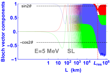
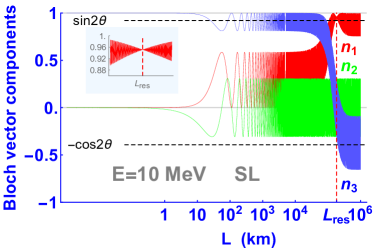
Figure 1: Components of the Bloch vector as a function of distance from the centre of the Sun, $L$, for 5 MeV (left) and 10 MeV (right) neutrino state, according to the strictly linear (SL) evolution equation (6) for two-flavour approximation with the $\nu_{e}$ in the initial state. The narrowing observed for the $n_{1}$ component at the ’resonance’ distance, $L_{\rm res}$, is shown in the inset. Dashed horizontal lines mark the values of components $n_{1}$ and $n_{3}$ corresponding to the pure state $\bm{\nu}_{2}=(\sin 2\theta,0,-\cos 2\theta)$.

Wolfenstein introduced two effective variables, reflecting matter effects in neutrino oscillations, namely the mixing angle, $\theta_{\rm eff,W}$, and the mass-squared difference, $\Delta m_{\rm eff,W}^{2}$. The effective mixing angle reaches the value $45^{\circ}$ at the ’resonance’ distance, which corresponds to the maximal mixing, i.e. $p_{ee}=p_{e\mu}=0.5$. According to the strictly linear formalism, and using (22) and (24), the effective mixing angle can be expressed in terms of the energy gap as simply as

$$\sin 2\theta_{\rm eff,W}(L)=\frac{d_{\rm W}(L_{\rm res})}{d_{\rm W}(L)}.$$ (26)

Function (26) and the evolution of the component $n_{1}$ of the Bloch vector are shown in Fig. 2 for two energies, 5 MeV and 10 MeV. The effective mixing angle near the centre of the Sun for $E=10$ MeV yields a few degrees only, which indicates that flavour mixing is far much smaller than in the vacuum (i.e., matter effects dominate). Next, the angle attains $45^{\circ}$ at the ’resonance’ distance and then asymptotically goes to the measured (vacuum) value as the Wolfenstein potential vanishes. The higher energy, the more accurately the following relation is approximated

$$\langle n_{1}\rangle\approx\sin 2\theta_{\rm eff,W}.$$ (27)

The effective mass-squared difference can also be directly expressed in terms of the energy gap

$$\Delta m_{\rm eff,W}^{2}(L)=2E\>d_{\rm W}(L)$$ (28)

and one can show, using (24), that $\Delta m_{\rm eff,W}^{2}$ goes to $\Delta m^{2}$ as the Wolfenstein potential vanishes (the product $\Delta m_{\rm eff,W}^{2}\,\sin 2\theta_{\rm eff,W}=\Delta m^{2}\,\sin 2\theta$ is energy independent).

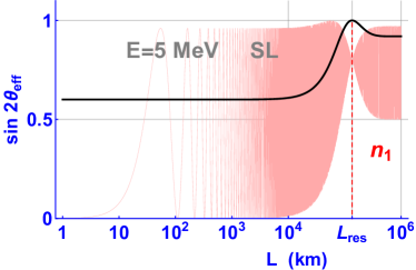
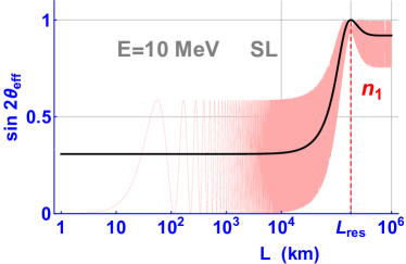
Figure 2: Effective mixing angle in matter, $\sin 2\theta_{\rm eff,W}$ (26), as a function of distance from the centre of the Sun, $L$, (solid line) superimposed on the component $n_{1}$ of the Bloch vector according to the strictly linear (SL) evolution equation (6) for two-flavour approximation with $\nu_{e}$ in the initial state, for 5 MeV (left) and 10 MeV (right) neutrino state.

Moreover, it can be numerically shown that the effective oscillation length of the neutrino state in the solar matter, $l_{\rm eff,W}$, again can be simply expressed in terms of the energy gap

$$l_{\rm eff,W}(L)=\frac{2\pi}{d_{\rm W}(L)}.$$ (29)

The effective oscillation length becomes that of free oscillations as the Wolfenstein potential vanishes, $l_{\rm eff,W}\rightarrow 2\pi/\omega_{0}$, where $\omega_{0}=\Delta m^{2}/2E$. Relations (26), (28) and (29) suggest that the effective mixing of neutrino flavour states and the character of oscillations in the solar matter is actually governed by the energy gap, i.e., the distance of the system from the structural instability point, while its minimal value sets a scale for the effective mixing angle. This interpretation illustrates the advantage of our approach to a deeper understanding of the dynamics underlying the linear evolution of neutrino flavour oscillations in the solar matter.

3.3 Quasilinear evolution of solar neutrinos

Now, we proceed to describe evolution of the neutrino state in the solar matter according to the quasilinear evolution equation (8). The subsystem-environment interaction is ascribed to the additional generator, $G$, appearing in Eq.8, hence it is justified to adopt only the free Hamiltonian in this case, $H_{\rm f}$ (cf. Appendix I)

$$H_{\rm f}=E\cdot I+\frac{\Delta m^{2}}{4E}\begin{pmatrix}-\cos 2\theta\;\;\;&\sin 2\theta\\ \sin 2\theta\;\;\;&\cos 2\theta\end{pmatrix}.$$ (30)

Vector $\bm{\omega}=\bm{\omega}_{0}$ then simply reads

$$\bm{\omega}_{0}=\left(\frac{\Delta m^{2}}{2E}\sin 2\theta,\>0,\>-\frac{\Delta m^{2}}{2E}\cos 2\theta\right).$$ (31)

Since the subsystem-environment interaction arises through the electron number density in the solar plasma, it is natural to contain it in the vector $\bm{g}$

$$\bm{g}(L)=g_{e}(L)\bm{e},$$ (32)

where $g_{e}(L)=\sqrt{2}{\rm G_{F}}n_{e}(L)$ and $\bm{e}$ is a unit vector. Note that the term "potential" is rather inadequate in reference to this case. It is convenient to express the scalar product $\bm{\omega}_{0}\bm{g}$ with the aid of a new angle $\sigma$

$$\bm{\omega}_{0}\bm{g}=\frac{\Delta m^{2}}{2E}\>g_{e}\cos\sigma$$ (33)

that leads to the following parametrisation of the unit vector

$$\bm{e}=\begin{pmatrix}\tfrac{\cos\sigma+\cos\eta\cos 2\theta}{\sin 2\theta}\\ \pm\tfrac{\sqrt{-\Big{(}\cos(\eta+2\theta)+\cos\sigma\Big{)}\Big{(}\cos(\eta-2\theta)+\cos\sigma\Big{)}}}{\sin 2\theta}\\ \cos\eta\end{pmatrix}.$$ (34)

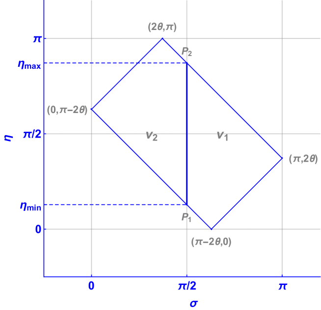
Figure 3: Rectangular space of parameters ($\sigma,\eta$), following from (34), (35). The thick vertical line marks the physical range of $\eta$ at $\sigma=\pi/2$ (transition line); coordinates of the vertices are shown in brackets.

Positive-definiteness of the expression under the square-root in (34) fixes the rectangular space of parameters for $\eta$ as shown in Fig. 3 in the range $[0,\pi]$. The vertical line at $\sigma=\pi/2$, corresponding to the perpendicular orientation of the vectors $\bm{\omega}_{0}$ and $\bm{g}$, distinguishes two extreme values of $\eta$ located at the boundary of the physical region

$$\eta_{\rm min}=\frac{\pi}{2}-2\theta;\;\;\;\;\;\eta_{\rm max}=\frac{\pi}{2}+2\theta$$ (35)

(points $P_{1}$ and $P_{2}$ in Fig. 3). The angles $\sigma$ and $\eta$ play an analogous role in the parametrisation of $\bm{g}$, i.e., fix its orientation in the lepton flavour space, like the mixing angle $\theta$ does for the parametrisation of $\bm{\omega}$. We note however that the angle $\sigma$ arises only in matter, i.e., when $\bm{g}\neq 0$ (33), and its vacuum value is physically undefined. Now, in view of (34), the invariants $C_{1}$ and $C_{2}$ (16) take the following form

$$C_{\rm 1,QL}(L)=\left(\frac{\Delta m^{2}}{2E}\right)^{2}-g_{e}^{2}(L)\;\;\;\;\;C_{\rm 2,QL}(L)=\frac{\Delta m^{2}}{2E}g_{e}(L)\cos\sigma(L),$$ (36)

and the corresponding energy gap (17) reads

$$d_{\rm QL}(L)=\Bigg{[}\;\Bigg{(}\Bigg{(}\frac{\Delta m^{2}}{2E}\Bigg{)}^{2}-g_{e}(L)^{2}\Bigg{)}^{2}+4\Bigg{(}\frac{\Delta m^{2}}{2E}g_{e}(L)\cos\sigma(L)\Bigg{)}^{2}\;\Bigg{]}^{\frac{1}{4}}.$$ (37)

Invariant $C_{1}$ vanishes for $L=L_{\rm ins}$ which fulfils the following condition

$$g_{e}(L_{\rm ins})=\frac{\Delta m^{2}}{2E}.$$ (38)

The relationship of $L_{\rm ins}$ and $L_{\rm res}$ follows from (23) and (38). Since $V_{e}(L_{\rm res})/g_{e}(L_{\rm ins})=\cos 2\theta$ and $n_{e}(L)$ is a decreasing function of $L$, the following relation holds: $L_{\rm ins}<L_{\rm res}$. For example, for $E=10$ MeV, $L_{\rm ins}\approx 118800$ km < $L_{\rm res}\approx 182800$ km. Invariant $C_{2}$ vanishes independently for $\sigma=\pi/2$. The threshold energy in this description results from the condition $C_{1}(0)=0$,

$$E_{\rm th,QL}=\frac{\Delta m^{2}}{2g_{e}(0)}\approx 3.09~{}{\rm MeV}.$$ (39)

The strictly perpendicular orientation of vectors $\bm{\omega}_{0}$ and $\bm{g}$ in the solar matter can be excluded on the experimental basis. Indeed, if $\sigma=\pi/2$, the oscillating neutrino state reaches the point $L=L_{\rm ins}$ at which both invariants vanish, $C_{1}=C_{2}=0$, and so does the energy gap, $d_{\rm QL}(L_{\rm ins})=0$ (37). One then has to do with maximal instability of the system caused by the structural instability point, in consequence of which the character of the evolution drastically changes, which manifests as follows. From the moment of neutrino creation at $L=0$, the oscillations are fully suppressed (see below) until the system reaches the structural instability point at which the evolution acquires a form of free oscillations for all three components of the Bloch vector. In particular the mean value of the third component of the Bloch vector amounts to zero, $\langle n_{3}\rangle=0$, corresponding to the survival probability $p_{ee}=0.5$, independently of energy (above threshold), in gross disagreement with the experimental results for $10$ MeV ⁸B neutrinos. Thus the evolving state of the system must omit the structural instability point by adopting a nonzero value of the invariant $C_{2,QL}~{}($36) which can be achieved if the value of the angle $\sigma$ differs from $\pi/2$. The transition line at $\sigma=\pi/2$ separates two regions on the $(\sigma,\eta)$ plane, denoted $\nu_{1}$ and $\nu_{2}$ in Fig. 3. If $\sigma<\pi/2$ the initial state $\bm{\nu}_{e}$ asymptotically converges to $\bm{\nu}_{2}$, as indicated the measurements on Earth, while would do to $\bm{\nu}_{1}$ in the opposite case. Such pattern is reminiscent of the existence of two separated phases, $\nu_{1}$ and $\nu_{2}$. Now, the key observation is that only when the value of $\sigma$ is contained within a narrow band about the transition line, approximately $10^{-2}$ rad wide, an energy-dependent prediction for the $\nu_{e}$ survival probability would result, in agreement with the measurements. We thus introduce a dimensionless perturbation parameter, $\delta<0$, to describe the deviation of the vectors $\bm{\omega}$ and $\bm{g}$ from perpendicularity. The effective angle $\sigma$ in the solar matter is then expressed as follows

$$\sigma=\frac{\pi}{2}+\delta$$ (40)

(as $\delta$ should vanish in the vacuum, the angle $\sigma$ accordingly would become $\pi/2$ which can be taken as a reference, not the vacuum value). Following (40), the Casimir invariant $C_{2}$ (36) can be written as $\bm{\omega}\bm{g}\approx|\bm{\omega}||\bm{g}|\,\delta$ which is a scalar under rotations in the flavour space. Bearing in mind Fig. 3 we note that if the value of $\eta$ is set to $\eta_{\rm max}$, only the minus sign in (40) is admissible since the plus sign would move the value of $\sigma$ beyond the physical region. Nevertheless, as separate studies have shown, the exact value of $\eta$ is not relevant for the current considerations.

In order to find a plausible formula for $\delta$, we argue along the following line. A nonzero value of $\delta$ arises due to a non-vanishing electron number density, except where it is constant and the instability point cannot be reached (e.g., terrestrial matter). This justifies assuming $\delta$ proportional to the gradient of the radial distribution of the electron number density (20), $\delta\propto h^{\prime}_{e}<0$. We adopt an effective parametrisation of $\delta$ in the solar energy range in a factorised form, as a product of three terms, $\delta(E,L)=C\,F(E)\,h^{\prime}_{e}(L)$, where $C$ is a constant factor of dimension ${\rm km}$ in order to account for the unit ${\rm km^{-1}}$ of the gradient, and $F(E)$ – a dimensionless function of the neutrino energy. The partial product of the first two terms, defined as $C_{F}(E)=C\,F(E)$, will also be used below. We assume the coefficient $C$ to be expressed in terms of the universal constants with an additional multiplicative factor $f$, in general depending on the mixing angle, serving to fulfill the criteria specified below. The function $F(E)$ is expressed in terms of a dimensionless ratio involving the quantities describing the system, i.e., $g_{e}(0)/\omega_{0}$ ($\omega_{0}=\Delta m^{2}/2E$).

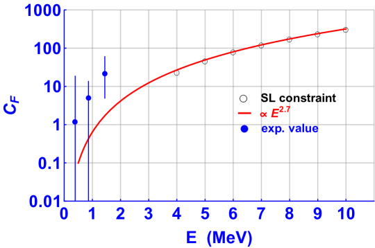
Figure 4: Empirical parametrisation of the function $C_{F}\propto E^{2.7}$ (41), determined by matching the $\delta$-dependent QL prediction for survival probability, $p_{ee}$, to points (open circles) representing the $p_{ee}$ values at discrete energies for the SL evolution (solid line); full points with error bars represent values of $C_{F}$ matching the experimental survival probability for pp, ⁷Be and pep neutrinos.

We parameterise the function $F(E)$, i.e., the energy dependence of $\delta$, in terms of a power $r$ of the ratio $g_{e}(0)/\omega_{0}$, yielding the following explicit formula

$$\delta(E,L)=f\,\frac{\hbar c}{g(0)}\left(\frac{g(0)}{\omega_{0}}\right)^{r}\;h^{\prime}_{e}(L),$$ (41)

where the parameter $r$ remains to be determined; note also that $g(0)/\omega_{0}=E/E_{\rm th,QL}$, where the threshold energy is given by (39). If accurate measurements of the neutrino survival probability were available in a range of energies, the value of the parameter $r$ could be determined experimentally. Meanwhile there is only one such useful constraint coming from the measurement at $E=10$ MeV for ⁸B neutrinos while those for pp, ⁷Be and pep neutrinos are of a limited value due to their very large uncertainties. We thus tentatively chose to determine an indicative value of $r$, obtained by demanding that certain predictions of the QL evolutions agree with those of the SL evolution; in particular, the mean asymptotic (as the electron number density becomes negligible) survival probability as a function of the neutrino energy, $p_{ee}(E)$ and its asymptotic oscillation amplitude (depth). It appeared that these criteria entailed also a good agreement of two other asymptotic quantities introduced hereunder – energy transfer and speed of the state evolution (Sec. 4.1 and 4.2). In order to determine the parameter $r$ and the coefficient $f$ we computed several values of $C_{F}(E)$ at discrete energies above the threshold ($4<E<10$ MeV) that lead to QL predictions matching those of the SL evolution, as detailed above ("SL constraint"). We fitted the resulting values with a function proportional to $E\,^{r}$, yielding $r\approx 2.7$, as shown in Fig. 4. An agreement of the depths of oscillations at asymptotic distances for the SL and QL evolutions can be achieved for $f\approx 0.82$. These particular values of $r$ and $f$ arise as a consequence of adopting the input values for $\Delta m^{2}$, $\theta$ and $g(0)$ specified earlier.

Aside from the above effective parametrisation, obtained relatively to the SL evolution, we independently determined the value of $C_{F}$ for each individual measured survival probability at low energies (pp, ⁷Be and pep neutrinos) in such a way that the QL prediction reproduces each experimental value, with uncertainties of $C_{F}$ resulting from matching the experimental values altered by the corresponding experimental uncertainty. These results are also shown Fig. 4 as experimental points with error bars and suggest that the $C_{F}$, i.e., $\delta$, is compatible below the threshold with the prediction following from (41).

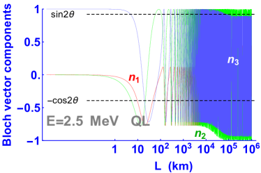
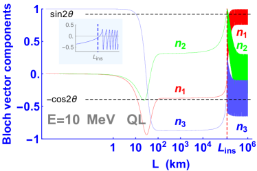
Figure 5: Components of the Bloch vector as a function of distance from the centre of the Sun, $L$, for a sub-threshold 2.5 MeV (left) and 10 MeV (right) neutrino state, according to the quasilinear evolution equation (12) with $\eta=\eta_{\rm max}$ and $\delta$ given by (41) and detailed in the text, for two-flavour approximation with the $\nu_{e}$ in the initial state. Details of the component $n_{3}$ about the instability point, $L_{\rm ins}$, are shown in the inset for $E=10$ MeV. Dashed horizontal lines mark the values of components $n_{1}$ and $n_{3}$ corresponding to the pure state $\bm{\nu}_{2}=(\sin 2\theta,0,-\cos 2\theta)$.

Evolution of the Bloch vector with $\delta$ given by (41) and $r=2.7$ is presented in Fig. 5 where the solution of (12) is shown for a sub-threshold energy $E=2.5$ MeV and for $E=10$ MeV ($\eta=\eta_{\rm max}$) and $\nu_{e}$ in the initial state. In the former case the evolution has a periodic but nonlinear character. For energies above the threshold, oscillations of all three components of the Bloch vector are suppressed inside the Sun and appear only as the system reaches the instability distance, $L_{\rm ins}$, and subsequently converge to a constant mean value, similarly as in the strictly linear case. The influence of the structural instability point on the evolution of the system for energies above threshold is manifested exactly by this sudden change of the character of the evolution, from non-oscillatory to oscillatory, shown in the inset for the component $n_{3}$. Again the asymptotic neutrino state is not the pure mass state $\nu_{2}$ but an oscillating state with the mean values of the components approximately corresponding to $\nu_{2}$. The electron neutrino survival probability, $p_{ee}(L)$, is also an oscillating function of $L$ as the electron number density vanishes. The component $n_{3}$ of the Bloch vector crosses zero at the instability distance and the mean $\nu_{e}$ survival probability amounts to 0.5 at this point (maximal mixing). Neither in this case the initial $\nu_{e}$ achieves the muon neutrino state during its evolution.

3.4 Comparison of linear and quasilinear evolutions

Since the $L$-dependent energy gap, i.e., distance of the system from the structural instability point, plays a key role in the evolution of state in both strictly linear and quasilinear descriptions, in Fig. 6 we compare the respective functions, given by equations (22) and (37).

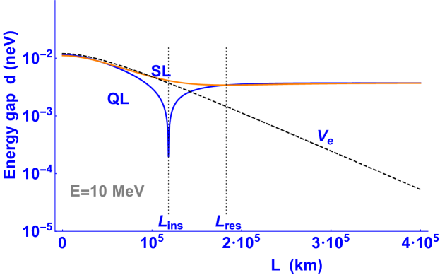
Figure 6: Energy gap (17) for strictly linear (SL) and quasilinear (QL) evolution of 10 MeV neutrino state; note the shallow minimum at $L_{\rm res}$ in the SL case. The Wolfenstein potential, $V_{e}$, is plotted on the same scale, marked by dashed line.

In the strictly linear case, the function $d_{\rm W}(L)$ exhibits a shallow minimum at $L=L_{\rm res}$. In the quasilinear case, the function $d_{\rm QL}(L)$ is characterised by a deep and sharp (but differentiable) minimum at $L=L_{\rm ins}$. Both functions have approximately the same values at $L=L_{\rm res}$ and converge to one common asymptotic $L$-dependence. Predictions for the third component of the Bloch vector for the linear and the quasilinear ($\eta=\eta_{\rm max}$) neutrino evolutions are compared in Fig. 7 for $\eta=\eta_{\rm max}$ and $\eta=\eta_{\rm min}+0.02$ (the value of $\eta$ near the minimum increased by a tiny amount to allow the angle $\sigma=\pi/2+\delta$ remain within the physical region). Mean values and depths of survival probabilities for both cases in the asymptotic limit can be brought to agreement by adjusting only the factor $f$ of the perturbation parameter $\delta$ (41). The two asymptotically oscillating functions are relatively shifted in phase (not resolved on the figure), however of no effect on the measurements on Earth.

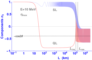
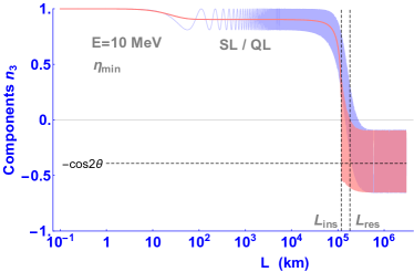
Figure 7: Comparison of the components $n_{3}$ of the Bloch vector as functions of distance from the centre of the Sun, $L$, for a 10 MeV neutrino state according to the strictly linear (SL) (6) and quasilinear (QL) (12) evolution with $r=2.7$ for $\eta=\eta_{\rm max}$ (left) and $\eta\approx\eta_{\rm min}$ (right). Distances of the structural instability point, $L_{\rm ins}$, and the ’resonance’ point, $L_{\rm res}$, are marked by dashed vertical lines. Dashed horizontal line marks the $n_{3}$ component of the Bloch vector corresponding to the pure state $\bm{\nu}_{2}=(\sin 2\theta,0,-\cos 2\theta)$.

Since measurements on Earth regard only the mean value of the asymptotic survival probability, an important information is delivered by its energy dependence, which is shown in Fig. 8. The energy dependence is monotonic in the strictly linear (SL) description and reaches the asymptotic value of approx. 0.3 for $E=10$ MeV. In the quasilinear (QL) description, using $\eta=\eta_{\rm max}$ and $\delta$ given by (41) with $r=2.7$, the energy dependence is distinctly different. One can observe an "ankle" at the threshold energy beyond which the survival probability tends towards an agreement with the strictly linear evolution (as was assumed). Adopting $\eta\approx\eta_{\rm min}$ for the QL evolution only insignificantly alters the predictions below the threshold.

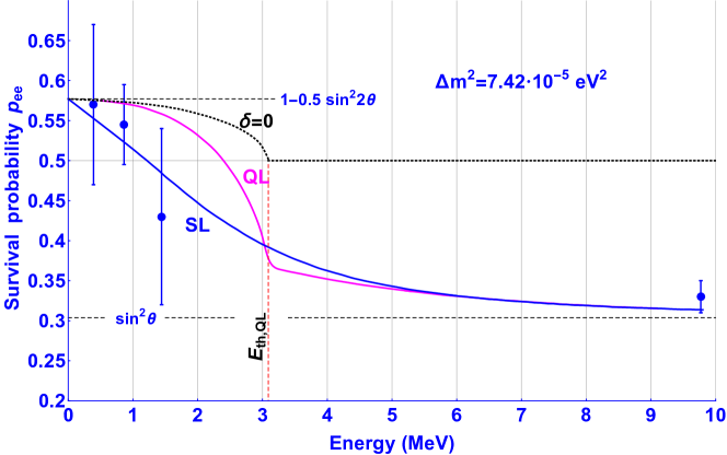
Figure 8: Predicted energy dependence of the neutrino survival probability, $p_{ee}$, for the strictly linear (SL) and quasilinear (QL) with $r=2.7$ ($\eta=\eta_{\rm max}$) evolution computed using $\Delta m^{2}=7.42\cdot 10^{-5}$ eV². Dashed horizontal lines mark the values for $E\rightarrow 0$ and $E\rightarrow\infty$, amounting to $p_{ee}=1-\frac{1}{2}\sin^{2}2\theta\approx 0.58$ and $p_{ee}=\sin^{2}\theta\approx 0.30$, respectively. Dashed vertical line indicates the threshold energy for the QL evolution, $E_{\rm th,QL}$, amounting to $3.09$ MeV (39). Prediction for $\delta=0$ is also shown (dotted line).

The "ankle" in the quasilinear evolution the threshold energy denotes a change in the energy dependence dynamics resulting from the transition between two contrasting evolution modes: oscillatory and non-oscillatory (cf. Fig. 5). The prediction for $\delta=0$ is also shown. Comparing any model with predictions of the linear formalism could be conclusive only if the precision of the data about the threshold, $1\div 4$ MeV, was significantly improved. This is very difficult to achieve since the neutrino flux is low in that energy range (mainly the pep and ${\rm{}^{7}Be}$ channels) in the presence of a significant radioactive background.

4 Neutrino in solar environment

4.1 Neutrino–Sun energy transfer

Given the Bloch vector, one can address a natural question in the context of open systems – mean energy transfer between the propagating neutrino and the Sun, intriguing despite an unmeasurable quantity involved, of the order of $\Delta m^{2}/4E$. The mean value of the kinetic part of the free Hamiltonian, $\langle H_{\rm kin}\rangle$ (cf. Appendix I), which corresponds to a difference of "kinetic terms" for mass eigenstates $m_{1}$ and $m_{2}$, is given by the standard quantum-mechanical formula

$$\langle H_{\rm kin}\rangle=\mathrm{Tr}\hskip 2.0pt(H_{\rm kin}\>\rho)=\frac{1}{2}\bm{\omega}_{0}\bm{n},$$ (42)

where $\rho$ is the density matrix, $\bm{\omega}_{0}$ is given by (31) and $\bm{n}=\bm{n}(L)$ is the Bloch vector obtained by solving (6) or (12), depending on the considered case. A comparison of both mean kinetic terms of the free Hamiltonians as a function of $L$ for the linear and quasilinear propagation is shown in Fig. 9a for $E=10$ MeV. Although functional dependencies differ inside the Sun, the average values in both descriptions reach the same limit as the electron number density vanishes, provided the asymptotic oscillation depths agree (independently of the parameter $\eta$ in the QL description). The value of $\langle H_{\rm kin}\rangle$ at the $\nu_{e}$ creation point, $L=0$, is negative and amounts to $\langle H_{\rm kin}\rangle=-(\Delta m^{2}/4E)\cos 2\theta$ while it reaches an almost asymptotic value of $\Delta m^{2}/4E$ as the neutrino state becomes the mean $\nu_{2}$ state. This finding indicates that the net gain of kinetic energy of the neutrino system is positive by an amount $(\Delta m^{2}/4E)(1+\cos 2\theta)$ after the state has made its way through the solar matter. According to the SL evolution, the increase occurs monotonically; in the QL description it is sharp and arises suddenly at the instability point $L=L_{\rm ins}$. The fact that the propagating neutrino and the Sun constitute an open system is more pronounced in the quasilinear description of the neutrino evolution.

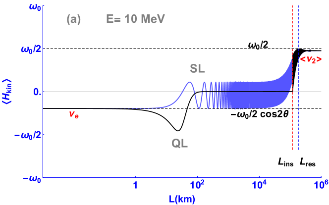
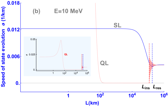
Figure 9: (a) Mean kinetic Hamiltonian, $\langle H_{\rm kin}\rangle$, in units of $\omega_{0}=\Delta m^{2}/2E$, as a function of the distance from the centre of the Sun, $L$, according to the strictly linear (SL) and quasilinear (QL) ($\eta=\eta_{\rm max}$) evolution in the solar matter for $E=10$ MeV neutrino state; $\nu_{e}$ and $\langle\nu_{2}\rangle$ denote the initial and the final states, the latter referring to its oscillating character with the mean Bloch vector corresponding approximately to that of the mass eigenstate $\nu_{2}$; (b) speed of the strictly linear (SL) and quasilinear (QL) state evolution (43) (km^-1); the full function for the QL evolution is shown on a separate scale in the inset.

4.2 Speed of the state evolution

In quantum information theory an important notion is the speed of the state evolution, denoted by $\vartheta$. Among different definitions cite:Wigner1 ; cite:Anandan1 ; cite:Brody2 ; cite:Campaioli1 (cf. Appendix II) the most natural and effective concept involves the time derivative of the Bloch vector which, adapted to the present formalism of two-flavour oscillations, leads to the following expression with time replaced by $L$ as the evolution parameter

$$\vartheta(L)=\sqrt{\frac{1}{2}\bm{n}^{\,\prime}(L)^{2}}.$$ (43)

Using (12) yields

$$\vartheta(L)=\tfrac{1}{\sqrt{2}}\sqrt{\bm{\omega}^{2}\bm{n}^{2}-(\bm{\omega}\bm{n})^{2}+\bm{g}^{2}+(\bm{n}^{2}-2)(\bm{g}\bm{n})^{2}+2(\bm{g}\times\bm{\omega})\bm{n}},$$ (44)

which for pure states ($\bm{n}^{2}=1$) reduces to

$$\vartheta_{\rm pure}(L)=\tfrac{1}{\sqrt{2}}\sqrt{\bm{\omega}^{2}-(\bm{\omega}\bm{n})^{2}+\bm{g}^{2}-(\bm{g}\bm{n})^{2}+2(\bm{g}\times\bm{\omega})\bm{n}},$$ (45)

leading to a simple formula in the case of the linear evolution ($\bm{g}=0$)

$$\vartheta_{\rm W}(L)=\tfrac{1}{\sqrt{2}}\sqrt{\bm{\omega}^{2}-(\bm{\omega}\bm{n})^{2}}$$ (46)

with $\bm{\omega}$ given by (7) and $\bm{n}$ being the solution of (6) with the initial condition $\bm{n}(0)=\bm{\nu}_{e}$. An analogous, though more complicated, formula can be obtained from (45) for the quasilinear evolution, with the aid of (31) and (32). The function (46), shown in Fig. 9b for $E=10$ MeV, has a minimum very near $L=L_{\rm res}$ and a certain asymptotic value. Thus for finite energies a minimal value of the evolution speed occurs near the ’resonance’ distance. However it can be checked using (46) that the value of the evolution speed would become zero with vanishing electron number density, should the asymptotic neutrino state become strictly $\nu_{2}$. This would be the case for asymptotic energies when the outgoing neutrino state becomes $\bm{\nu}_{2}=(\sin 2\theta,0,-\cos 2\theta)$. Meanwhile, also the minimum would disappear as the evolution speed would decrease and remain zero beyond the ’resonance’ distance. On the other hand, the higher energy, the better does the asymptotic neutrino state approximate the $\nu_{2}$ state.

The speed of the state evolution and the effective oscillation length in the linear picture (29) are numerically connected as follows

$$l_{\rm eff,W}(L)=\frac{\sqrt{2}}{\vartheta_{\rm W}(L)}$$ (47)

and thus the relation

$$\vartheta_{\rm W}(L)=\frac{d_{\rm W}(L)}{\sqrt{2}\pi}$$ (48)

repeatedly supports the interpretation that the speed of the evolution of state is driven by the energy gap, $d_{\rm W}(L)$.

5 Summary, discussion and conclusions

We presented a new description of neutrino propagation in the solar matter starting from the assumption that the whole is an open system due to the weak interactions. In consequence we exploited the von Neumann equation modified by way of a quasilinear extension, allowed by quantum mechanics for open systems cite:RC1 . In the resulting evolution equation (12) for the Bloch vector of the neutrino state, $\bm{n}(L)$, interactions of neutrinos were described through the Hamiltonian, $H$, and an additional generator, $G$, containing information about the neutrino interactions with the solar environment. We discussed the solutions for the Bloch vector in the context of $\mathsf{SL(2,C)}$ covariance group of this system. The Casimir invariants $C_{1}$ and $C_{2}$ of $\mathsf{SL(2,C)}$ determine the energy gap, $d(L)$ (17), i.e., an interval in the space of invariants, characterising structural instability and ’resonance’ points of equation (12) as well as the magnitude of the influence of the structural instability point on the evolution of the system. It was shown that the structural instability point should be identified with the configuration $(C_{1},C_{2})=(0,0)$ while the ’resonance’ point is obtained by minimising the energy gap (22) (Fig. 6).

We first applied this extended formalism to the strictly linear (SL) von Neumann equation with the Hamiltonian (2) containing the interaction part specified by the Wolfenstein potential. We solved Eq. 6 in the two-flavour approximation, with the initial condition corresponding to the electron-neutrino. The SL von Neumann equation is a special case of the quasilinear equation (12) with $G=0$. We obtained the Bloch vector comprising the complete information about the evolution of the system during propagation in the solar matter. The change of the locally averaged survival probability near the ’resonance’ point (Fig. 1) can be interpreted as due to the influence of the structural instability point.

Next we focused on solutions of the modified von Neumann equation (12) in which terms involving the additional generator $G$ were preserved, resulting in its quasilinearity. We restricted ourselves to the case of a free Hamiltonian (30) with the neutrino interactions with the environment contained solely in the generator $G$ via the flavour vector $\bm{g}_{e}(L)$ (32). The principal feature of the QL evolution described by (12) under the above choice is such that the survival probability inside the Sun, $L<L_{\rm ins}$, is a non-oscillating function of $L$ which can be interpreted, according to the classical nomenclature, as characteristic for a strongly damped (overdamped) system. In this case the structural instability point can be reached during evolution of the system, $C_{1}(L_{\rm ins})=C_{2}(L_{\rm ins})=0$, when the flavour vectors $\bm{\omega}$ and $\bm{g}$ are perpendicular. In order to make the system bypass this point it is necessary to introduce an energy and $L$-dependent perturbation, $\delta$, to the direction of the vector $\bm{g}$, fixing the orientation of the generator $G$ in the flavour space. We proposed an ansatz for $\delta$ (41) which assures almost the same $\nu_{e}$ survival probability at the highest measured energy point (10 MeV) as in the SL case. The differences between the SL and QL approaches may be possibly observed in the detailed energy dependence for neutrino energies below and about the threshold, i.e., in the energy range $1\div 4$ MeV (Fig. 8). However, obtaining corresponding measurements of the neutrino survival probability with small uncertainties is challenging. We underline that in both, SL and QL, cases the neutrinos leaving the Sun are not in the pure $\nu_{2}$ state but in a state for which the locally averaged $\nu_{e}$ survival probability is nearly the same as for $\nu_{2}$. This can be seen from the Fig. 1 and Fig. 5 where the evolution of the neutrino state is presented and oscillations in the asymptotic state are evident.

We have shown that a distinguished distance, appearing in the SL description, denoted $L_{\rm res}$, corresponds to a minimum of the energy gap or a maximum of the effective mixing angle (Fig. 2), however assigning a resonant character to these aspects of evolution is too far reaching. As regards the "adiabatic flavour conversion", indicated in the literature on the MSW effect, the formalism based on the density matrix does not require introducing such concepts. The initial state $\nu_{e}$ evolves throughout the entire trajectory of the neutrino state in the Sun and ends up in an oscillating state with mean values of the Bloch vector components corresponding to the state $\nu_{2}$.

We have also dealt with two new related issues. One effect, although interesting but rather unmeasurable, is energy transfer in the neutrino flux on the way through the solar matter. From Fig. 9(a) it follows that during propagation inside the Sun the neutrino gains ’kinetic’ energy, i.e., energy is transferred to it from the environment, irrespectively of the SL or QL character of the evolution. This observation supports the open system scenario worked out in this paper. However, the gap between the outgoing neutrino mean energy and the maximal energy which corresponds to the state $\nu_{2}$ supports the earlier conclusion that the outgoing state is near but not identical with $\nu_{2}$. The other study regarded the speed of the neutrino state evolution. Indeed, one can see from Fig. 9(b) that the asymptotic speed of the outgoing state is different from zero which should be the case for the pure state $\nu_{2}$. Each of the above quantities, obtained from the strictly linear and quasilinear equations, respectively, are in agreement in the limit of the vanishing solar electron number density.

As a general conclusion, we have demonstrated that the evolution of the neutrino state in the solar matter, aside from the MSW formalism, can be also described in terms of a quasilinear evolution equation, resulting from treating the neutrino and the Sun as an open system. Both approaches lead to similar results for the survival probability on Earth, with predictions notably different inside the Sun. Thus for obvious reasons it cannot be resolved by a direct measurement which one is proper in the solar scenario. A hope to achieve this in an indirect way, through the energy dependence of the survival probability, is rather faint. One can however search for signatures of the quasilinear evolution in the past and future terrestrial experiments with known baselines and beams passing through the Earth’s mantle.

6 Appendices

6.1 Appendix I

Under the assumption of constancy of the neutrino momentum, neutrino kinetic energies $E_{i}=\sqrt{p^{2}+m_{i}^{2}}$ are eigenvalues of the free Hamiltonian, $H_{\rm free}$, which takes the following form in the flavour basis (without approximations)

$$H_{\rm free}=E\cdot I+H_{\rm kin}$$ (49)

where $I$ is the identity matrix, $E$ is the mean energy, i.e., $E=\tfrac{1}{2}(E_{1}+E_{2})$ and $H_{\rm kin}$ denotes the "kinetic" part of the free Hamiltonian

$$H_{\rm kin}=\frac{\Delta m^{2}}{4E}\begin{pmatrix}-\cos 2\theta\hskip 14.22636pt&\sin 2\theta\\ \sin 2\theta\hskip 14.22636pt&\cos 2\theta\end{pmatrix}.$$ (50)

The full Hamiltonian includes the interaction term, $H_{\rm int}$, which can be rewritten in the flavour basis as follows

$$H_{\rm int}=\begin{pmatrix}V_{e}(L)\hskip 14.22636pt&0\\ 0\hskip 14.22636pt&0\end{pmatrix}=\frac{V_{e}(L)}{2}\cdot I+\frac{1}{2}\begin{pmatrix}V_{e}(L)\hskip 8.53581pt&0\\ 0\hskip 8.53581pt&-V_{e}(L)\end{pmatrix}.$$ (51)

Thus the full Hamiltonian, $H_{\rm tot}=H_{\rm free}+H_{\rm int}$, reads

$$H_{\rm tot}(L)=\left(E+\frac{V_{e}(L)}{2}\right)\cdot I\\ +\frac{1}{2}\begin{pmatrix}-\tfrac{\Delta m^{2}}{2E}\cos 2\theta+V_{e}(L)&\sin 2\theta\\ \sin 2\theta&\tfrac{\Delta m^{2}}{2E}\cos 2\theta-V_{e}(L)\end{pmatrix},$$ (52)

where the second term is identified as the Wolfenstein Hamiltonian. The term proportional to the unit matrix in (52) drops out from the von Neumann equation (5) as a result of commutation properties of the unit matrix leading to the traceless MSW Hamiltonian (2). For any value of $L$, neutrino energy varies between the eigenvalues $E_{\pm}(L)$ of the Hamiltonian (52)

$$E_{\pm}(L)=\left(E+\frac{V_{e}(L)}{2}\right)\pm\frac{1}{2}\sqrt{\left(\frac{\Delta m^{2}}{2E}\sin 2\theta\right)^{2}+\left(V_{e}(L)-\frac{\Delta m^{2}}{2E}\cos 2\theta\right)^{2}},$$ (53)

where the square root term, cf. (3), determines the limits of the energy range and can be written as $\pm\frac{1}{2}\sqrt{C_{1}(L)}$ (21). As the Wolfenstein potential vanishes, the energy range (53) reaches

$$E_{\pm}=E\pm\frac{\Delta m^{2}}{4E}.$$ (54)

In a general case the eigenvalues of the generator (14)

$$H+iG=\frac{1}{2}(\bm{\omega}+i\bm{g})\bm{\sigma}$$ (55)

are complex and take the form

$$\lambda_{\pm}=\pm\frac{1}{2}\sqrt{(\bm{\omega}^{2}-\bm{g}^{2})+2i\bm{\omega}\bm{g}}=\pm\frac{1}{2}\sqrt{C_{1}(L)+2iC_{2}(L)}\equiv\pm\lambda(L)$$ (56)

while the energy gap (17) can be written as

$$d(L)=\left((\bm{\omega}^{2}-\bm{g}^{2})^{2}+4(\bm{\omega}\bm{g})^{2}\right)^{\frac{1}{4}}=\left(C_{1}(L)^{2}+4C_{2}(L)^{2}\right)^{\frac{1}{4}}=2|\lambda_{\pm}|$$ (57)

and then $E_{+}-E_{-}=d(L)$ at a given energy, $E$. We also note that, since ${\rm Tr}\rho=1$, any term proportional to the unit matrix in an expansion of the generator $G$ drops out from the modified von Neumann equation too.

6.2 Appendix II

The most natural and effective definition of the speed of the state evolution is the following

$$\vartheta(t)=\sqrt{\mathrm{Tr}(\partial_{t}\rho)^{2}}.$$ (58)

In the case of ${\rm n}$-dimensional Hilbert space the density matrix, $\rho$, can be represented as

$$\rho=\frac{1}{\mathrm{n}}\Bigg{(}I+\sum_{\alpha=1}^{\mathrm{n}^{2}-1}n_{\alpha}\lambda_{\alpha}\Bigg{)},$$ (59)

where $\lambda_{\alpha}$ are the generalised Hermitian, traceless Gell-Mann matrices with $\mathrm{Tr}(\lambda_{\alpha}\lambda_{\beta})=\delta_{\alpha\beta}$. The components $n_{\alpha}$ of the generalized, ${\rm n}^{2}-1$-dimensional, Bloch vector $\bm{n}$, are real and $\bm{n}^{2}=\sum_{\alpha=1}^{{}\rm n^{2}-1}n_{\alpha}\leq 1$, which constitutes the Euclidean norm in the convex space of Bloch vectors. By means of (59), the speed (58) takes the form

$$\vartheta=\sqrt{\frac{1}{\mathrm{n}}\dot{\bm{n}}^{2}}.$$ (60)

Adapted to the solar neutrino case of $L$-dependent density matrix, $\rho(L)$, evolution speed $\vartheta(L)$, with the distance $L$ as the evolution parameter, can be expressed as

$$\vartheta(L)=\sqrt{\frac{1}{\mathrm{n}}\bm{n}^{\,\prime}(L)^{2}}.$$ (61)

Now, by means of (8), equation (61) can be written as

$$\vartheta(L)=\sqrt{\mathrm{Tr}\Big{(}\partial_{L}\rho(L)\Big{)}^{2}}=\\ \sqrt{2\Bigg{(}\mathrm{Tr}\Big{(}(G^{2}+H^{2})\rho^{2}\Big{)}+\mathrm{Tr}(G\rho)^{2}-\mathrm{Tr}(H\rho)^{2}+i\mathrm{Tr}([H,G]\rho^{2})-2\mathrm{Tr}(G\rho^{2})^{2}\Bigg{)}}$$ (62)

(agreeing units requires accounting for the $\hbar c$ term on the r.h.s. of the above and the following equalities). In particular, for a pure state, $\rho^{2}=\rho$, (62) can be simplified

$$\vartheta_{\rm pure}(L)=\sqrt{\mathrm{Tr}\Big{(}\partial_{L}\rho(L)\Big{)}^{2}}=\\ \sqrt{2\Big{(}\mathrm{Tr}(H^{2}\rho)-\mathrm{Tr}(H\rho)^{2}+\mathrm{Tr}(G^{2}\rho)-\mathrm{Tr}(G\rho)^{2}+i\mathrm{Tr}([H,G]\rho)\Big{)}}.$$ (63)

For unitary evolution, $G=0$, one obtains from (43)

$$\vartheta(L)=\sqrt{2\Big{(}\mathrm{Tr}(H^{2}\rho)-\mathrm{Tr}(H\rho)^{2}\Big{)}}$$ (64)

while

$$\vartheta_{\rm pure}(L)=\sqrt{2\Big{(}\mathrm{Tr}(H^{2}\rho)-\mathrm{Tr}(H\rho)^{2}\Big{)}}$$ (65)

Finally, note that in all the above cases applied to the two-level quantum systems (two-flavour oscillation) described by a density matrix of the form (4) an extremely simple formula for $\vartheta$ (46) results

$$\vartheta_{\rm pure}(L)=\sqrt{\tfrac{1}{2}\bm{n}^{\,\prime}(L)^{2}}.$$ (66)

References

- (1) L. Wolfenstein, Neutrino oscillations in matter, Phys. Rev. D 17 (1978) 2369
- (2) L. Wolfenstein, Neutrino oscillations and stellar collapse, Phys. Rev. D 20 (1979) 2634
- (3) S.P. Mikheev, A.Y. Smirnov, Resonance Amplification of Oscillations in Matter and Spectroscopy of Solar Neutrinos, Sov. J. Nucl. Phys. 42 (1985) 913; Yad. Fiz. 42 (1985) 1441
- (4) S.P. Mikheev and A.Y. Smirnov, Resonant amplification of neutrino oscillations in matter and solar neutrino spectroscopy, Nuovo Cim. C 9 (1986) 17
- (5) S.P. Mikheev and A.Y. Smirnov, Neutrino oscillations in an inhomogeneous medium: adiabatic regime, Sov. Phys. JETP 65 (1987) 230
- (6) S.P. Mikheev and A.Y. Smirnov, Resonant neutrino oscillations in matter, Prog. Part. Nucl. Phys. 23 (1989) 41
- (7) M. Maltoni and A. Yu. Smirnov, Solar neutrinos and neutrino physics, Eur. Phys. J. A 52 (2016) 87 [hep-ph/1507.05287]
- (8) H.-P. Breuer and F. Petruccione, The Theory of Open Quantum Systems, Oxford University Press, ISBN 978-0-1985-2063-4 (2020)
- (9) J. Rembieliński and P. Caban, Nonlinear extension of the quantum dynamical semigroup, Quantum 5 (2021) 420 [quant-ph/2003.09170]
- (10) J. Rembieliński and P. Caban, Nonlinear evolution and signalling, Phys. Rev. Research 2 (2021) 012027 [quant-ph/1906.03869]
- (11) R. Alicki and K. Lendi, Quantum dynamical Semigroups and Applications, 2nd edition Springer-Verlag, Berlin (2007)
- (12) K. Kowalski and J. Rembieliński, Integrable nonlinear evolution of the qubit, Ann. Phys. 411 (2019) 167955
- (13) N. Gisin, A simple nonlinear dissipative quantum evolution equation, J. Phys. A: Math. Gen. 14 (1981) 2259
- (14) D. C. Brody and E.-M. Graefe, Mixed-state evolution in the presence of gain and loss, Phys. Rev. Lett. 109 (2012) 230405 [quant-ph/1208.5297]
- (15) K. Kawabata, Y. Ashida, and M. Ueda, Information retrieval and criticality in parity-time symmetric systems, Phys. Rev. Lett. 119 (2017) 190401 [quant-ph/1705.04628]
- (16) V. I. Arnold, V. S. Afrajmovich, Yu. S. Ilyashenko, and L. P. Shilniov, Bifurcation Theory, Vol. 5, Springer-Verlag, Berlin- Heidelberg, 1994
- (17) S. Wiggins, Global Bifurcation and chaos, Analytical Methods, Springer-Verlag, New York (1988)
- (18) M. P. Decowski (KamLAND Collaboration), KamLAND’s precision neutrino oscillation measurements, Nucl. Phys. B 908 (2016) 52
- (19) Y. Nakajima, SuperKamiokande, talk given at the XXIX International Conference on Neutrino Physics and Astrophysics, Chicago, U.S.A., June 22 - July 2, 2020 (online conference)
- (20) I. Esteban et al., The fate of hints: updated global analysis of three-favor neutrino oscillations, JHEP 9 (2020) 178
-
(21)
J. N. Bahcall, A. M. Serenelli and S. Basu, http://www.sns.ias.edu/jnb/
SNdata/Export/BS2005/bs05_agsop.dat [astro-ph/0412440] - (22) F. Vissani, Joint analysis of Borexino and SNO solar neutrino data reconstruction of the survival probability, Nucl. Phys. and Atomic Energy 18 (2017) 303 [hep-ph/1709.05813]
- (23) E. P. Wigner and M. M. Yanase, Information contents of distributions, Proc. Nat. Acad. Sci. USA 49 (1963) 910
- (24) J. Anandan and Y. Aharonov, Geometry of Quantum Evolution, Phys. Rev. Lett. 65 (1990) 1697
- (25) D. C. Brody and B. Longstaff, Evolution speed of open quantum dynamics, Phys. Rev. Research 1 (2019) 033127 [quant-ph/1906.04766]
- (26) F. Campaioli, F. A. Pollock, and K. Modi, Tight, robust, and feasible quantum speed limits for open dynamics, Quantum 3, (2019) 168 [quant-ph/1806.08742]