HyperTree Proof Search for Neural Theorem Proving

Abstract

We propose an online training procedure for a transformer-based automated theorem prover. Our approach leverages a new search algorithm, HyperTree Proof Search (HTPS), inspired by the recent success of AlphaZero. Our model learns from previous proof searches through online training, allowing it to generalize to domains far from the training distribution. We report detailed ablations of our pipeline’s main components by studying performance on three environments of increasing complexity. In particular, we show that with HTPS alone, a model trained on annotated proofs manages to prove $65.4\%$ of a held-out set of Metamath theorems, significantly outperforming the previous state of the art of $56.5\%$ by GPT-f. Online training on these unproved theorems increases accuracy to $82.6\%$. With a similar computational budget, we improve the state of the art on the Lean-based miniF2F-curriculum dataset from $31\%$ to $42\%$ proving accuracy.

1 Introduction

Over the course of history, the complexity of mathematical proofs has increased dramatically. The nineteenth century saw the emergence of proofs so involved that they could only be verified by a handful of specialists. This limited peer review process inevitably led to invalid proofs, with mistakes sometimes remaining undiscovered for years (e.g. the erroneous proof of the Four Colour Conjecture [1]). Some mathematicians argue that the frontier of mathematics has reached such a level of complexity that the traditional review process is no longer sufficient, envisioning a future where research articles are submitted with formal proofs so that the correctness can be delegated to a computer [2].

Unfortunately, very few mathematicians have adopted formal systems in their work, and as of today, only a fraction of existing mathematics has been formalized. Several obstacles have hindered the widespread adoption of formal systems. First, formalized mathematics are quite dissimilar from traditional mathematics, rather closer to source code written in a programming language, which makes formal systems difficult to use, especially for newcomers. Second, formalizing an existing proof still involves significant effort and expertise (the formalization of the Kepler conjecture took over 20 person years to complete [3]) and even seemingly simple statements sometimes remain frustratingly challenging to formalize.

To write a formal proof, mathematicians typically work with Interactive Theorem Provers (ITPs). The most popular ITPs provide high-level “tactics” that can be applied on an input theorem (e.g. the initial goal) to generate a set of subgoals, with the guarantee that proving all subgoals will result in a proof of the initial goal (reaching an empty set means the tactic solves the goal). An example of a proof in Lean [4], an interactive theorem prover, is given in Figure 1 and the corresponding proof hypertree is illustrated in Figure 3. A tactic, induction k, is applied on the root goal ($n+k\leq m+k$) to start a proof by induction . The formal system returns two subgoals: $n+0\leq m+0$ (the initial case) and $n+k\leq m+k\Rightarrow n+k+1\leq m+k+1$ (the induction step). As the first subgoal is our initial hypothesis, it can be solved using the exact tactic. To prove the second subgoal, we first rewrite it using nat.succ_le_succ_iff, a theorem from the Lean library stating that $m+1\leq n+1\iff m\leq n$. The new subgoal then becomes our induction hypothesis $n+k\leq m+k$, and can again be solved using the exact tactic, thereby solving the last remaining subgoal and completing the proof of the initial statement. Starting from a goal and reducing it to subgoals until these can be solved, is commonly referred to as backward proving.

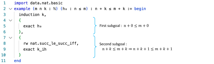
Figure 1: A simple proof of the statement $\mathbf{n\leq m\Rightarrow n+k\leq m+k}$ in Lean. The induction tactic reduces the initial statement to two subgoals, that can be solved independently.

In this paper, we aim at creating a prover that can automatically solve input theorems by generating a sequence of suitable tactics without human interaction. Such a prover could significantly reduce the effort required to formalize existing mathematics. The backward procedure naturally suggests a simple approach where a machine learning model trained to map goals to tactics interacts with an ITP to build the proof of an input goal in a backward fashion. The automated prover builds a hypergraph with the theorem to be proved as the root node, tactics as edges and subgoals as nodes. The prover recursively expands leaves by generating tactics with our model until we find a proof of the initial theorem. A proof in this setup is a hypertree rooted in the initial theorem whose leaves are empty sets. As many different tactics can be applied to a goal, and each tactic application can result in multiple subgoals, the number of goals in the graph grows exponentially and it is critical to reduce the search to the most promising branches. This can be done through techniques like alpha-beta pruning [5] or Monte Carlo Tree Search (MCTS) [6], known for its recent successes in difficult two player games [7]. However, challenges arise in search algorithms for theorem proving that do not occur in two player games. For instance:

• The action space, i.e. the amount of possible “moves” in a given state, is infinite (there is an unlimited number of tactics that can be applied to a given theorem). This requires sampling possible actions from a language model for which training data is scarce. Moreover, if all tactics sampled at a goal fail, we have no information on what region of the probability space to sample next.

• In the context of theorem proving, we need to provide a proof of all subgoals created by a tactic, whereas AlphaZero for two player games is allowed to focus on the most likely adversary moves.

• In Chess or Go, playing a sub-optimal move does not necessarily lead to losing the game, thus exploring these branches can provide information. In theorem proving, it is frequent to generate tactics that result in subgoals that can no longer be proved and on which the model will waste significant search budget.

This paper presents an in-depth study of our approach to overcome these difficulties and the resulting model, Evariste. In particular, we make the following contributions:

• A new MCTS-inspired search algorithm for finding proofs in unbalanced hypergraphs.

• A new environment (Equations) to easily prototype and understand the behavior of the models we train and our proof search.

• A detailed ablation study and analysis of the different components used in our approach on three different theorem proving environments. We study how data is selected for training the policy model after a successful or failed proof-search, what target should be used to train the critic model, and the impact of online training vs. expert iteration.

• State-of-the-art performance on all analyzed environments. In particular, our model manages to prove over $82.6\%$ of proofs in a held-out set of theorems from set.mm in Metamath, as well as $58.6\%$ on miniF2F-valid [8] in Lean.

We begin by introducing related work in Section 2 and present the three theorem proving environments that we study in Section 3. Then, we present our proof-search algorithm in Section 4, our online training pipeline in Section 5, and all experimental details in Section 6. Finally, we describe our main results and ablation studies in Section 7 before concluding in Section 8.

2 Related work

Automated theorem proving has been a long-standing goal of artificial intelligence, with the earliest work dating from the 1950s [9, 10]. Early approaches focused on simpler logics, culminating in extremely efficient first-order provers such as E [11] or Vampire [12]. However, these approaches are insufficient when it comes to theorems written in modern proof assistants such as Isabelle [13], Coq [14], or Lean [4]. Recently, the rising success of deep language models [15] and model-guided search methods [7] has spurred a renewed interest in the problem of automated theorem proving.

Neural theorem provers.

Recent work applying deep learning methods to theorem proving [16, 17, 18] are the closest to this work and obtained impressive results on difficult held-out sets for Metamath and Lean. The main differences between their approach and ours are the proof-search algorithm we propose, the training data we extract from proof-searches and our use of online training compared to their expert iterations. We validate experimentally that these differences lead to improved performances as well as faster training times. Another similar approach is Holophrasm [19], which is based on a different tree exploration technique which expands paths in an AND/OR tree, while we expand entire proof subtrees in a proof hypergraph. Their model is only trained once from supervised data and does not benefit from online training or expert iteration, which we found to be critical. DeepHOL [20] focuses on the HOL-Light environment [21]. Their model relies on a classifier that can select among a restricted set of tactics and arguments, while we rely on a seq2seq model that can generate arbitrary tactics. The suggested tactics are then used in a breadth-first search. TacticToe [22] uses an MCTS without learned components, using ranking on predefined features to guide the search. Machine learning has also been used to improve classical provers by re-ranking clauses [23]. Overall, previous studies always focus on a single proving environment (e.g. Metamath, Lean, or HOL-Light).

Reasoning abilities of language models.

Impressive performance of large language models in one or few shot learning [15], machine translation [24] or more recently code generation [25] spurred interest into the reasoning capabilities of large transformers. These model perform quite well on formal tasks such as expression simplification [26], solving differential equations [27], symbolic regression [28, 29], or predicting complex properties of mathematical objects [30]. These studies suggest that deep neural networks are well adapted to complex tasks, especially when coupled with a formal system for verification.

MCTS and two player games.

Recently, AlphaZero [7] demonstrated good performances on two player games, replacing the Monte-Carlo evaluations of MCTS [6] with evaluations from a deep neural network and guiding the search with an additional deep policy. This recent success follows extensive literature into search methods for two player games, notably alpha-beta search [5]. Theorem proving can be thought of as computing game-theoretic value for positions in a min/max tree: for a goal to be proven, we need one move (max) that leads to subgoals that are all proven (min). Noticing heterogeneity in the arities of min or max nodes, we propose a search method that goes down simultaneously in all children of min nodes, such that every simulation could potentially result in a full proof-tree.

3 Proving environments

In this paper, we develop and test our methods on three theorem proving environments: a) Metamath, b) Lean and c) Equations. Metamath [31] comes with a database of $30k$ human-written theorems called set.mm. We also evaluate our methods on the Lean proving environment, which provides a level of automation that is helpful to solve more complex theorems. Lean comes with a human-written library of $27k$ theorems called Mathlib [32]. Finally, since Metamath proofs can be quite difficult to understand and Lean requires more computing resources, we developed our own environment called Equations, restricted to proofs of mathematical identities. Its simplicity makes it ideal for prototyping and debugging. We briefly introduce these environments below.

3.1 Metamath

Metamath’s only rule is string substitution. Starting from a theorem to be proven, variables are substituted until we reach axioms. In our setup, we consider a tactic to be the label of a theorem in set.mm, along with the necessary substitutions. As shown in Figure 2, to show that $2+2=4$, the first step uses eqtr4i which states that $A=B\wedge C=B\Rightarrow A=C$ with substitutions: $A=(2+2)$, $B=(2+(1+1))$, and $C=4$. We are then left with two subgoals to prove: $(2+2)=(2+(1+1))$ and $4=(2+(1+1))$.

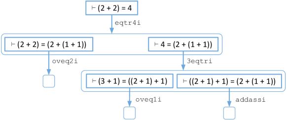
Figure 2: A visualization of the proof-tree for $\mathbf{2+2=4}$ in Metamath.

The simplicity of Metamath makes it a great test bed for our algorithms. However, its lack of automation leads to larger proof sizes and its syntax and naming conventions make each step difficult to interpret for neophytes. Similar to GPT-f, we implement a parser for Metamath in order to automatically prove the syntactic correctness of statements. Moreover, we use this parser to allow generating only substitutions that cannot be inferred from the goal.

3.2 Lean

Lean is a full-fledged programming language and benefits from more powerful automation than Metamath, with tactics such as ring (able to prove goals using manipulations in semirings), norm_num (able to prove numerical goals) or linarith (able to find contradictions in a set of inequalities). An example of a Lean proof-tree is shown in Figure 3.

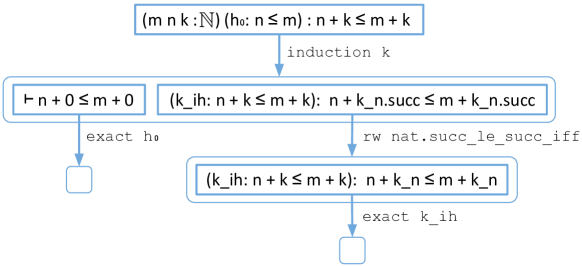
Figure 3: A visualization of the proof-tree for the proof discussed in the introduction in Lean.

States are more complex in Lean than in Metamath: metavariables can appear which are holes in the proof to be filled later. Subgoals sharing a metavariable cannot be solved in isolation. This is addressed in Polu and Sutskever [16] by using as input the entire tactic state. Instead, we inspect tactic states to detect dependencies between subgoals, and split the tactic state into different subgoals where possible in order to maximize state re-use and parallelization in the proof search algorithm.

Finally, Lean’s kernel type checker has to be called after each tactic application as tactics sometimes generate incorrect proofs and rely on the kernel for correctness. For every goal in the previous tactic state, we type check the proof term inserted by the tactic. Since the kernel does not support metavariables, we replace every metavariable by a lambda abstraction.

3.3 Equations

We developed the Equations environment as a simpler analogue to existing proving environments. Its expressivity is restricted to manipulating mathematical expressions (e.g. equalities or inequalities) with simple rules (e.g. $A+B=B+A$, or $A<B\Rightarrow-B<-A$). This reduced expressivity makes goals and tactics easy to understand, helping with interpretability and debugging: plotting the set of goals explored during a Metamath proof search does not give a lot of insights on whether it is on track to find a proof. In Section B of the appendix, we give an in-depth presentation of this environment, of how we represent goals (Section B.1), tactics (Section B.2) and how we prove statements (Section B.3).

Unlike in Metamath or Lean, we do not have access to a training set of human annotated proofs for this environment. Instead, we create a training set composed of randomly generated synthetic theorems and their proofs (see Sections B.6 and B.6 for details), and manually create an out-of-domain set of non-trivial mathematical identities for which we do not provide proofs, e.g. $\cosh(3x)=4\cosh(x)^{3}-3\cosh(x)$ or $\sin(4x)=(4\sin(x)-8\sin(x)^{3})\cos(x)$. We refer to this evaluation split as Identities, a set of 160 mathematical expressions.

As synthetic theorems randomly generated are much simpler and significantly differ from statements in the Identities split, we can evaluate the ability of our model to generalize to complex and out of domains data. An example proof-tree in Equations is shown in Figure 4.

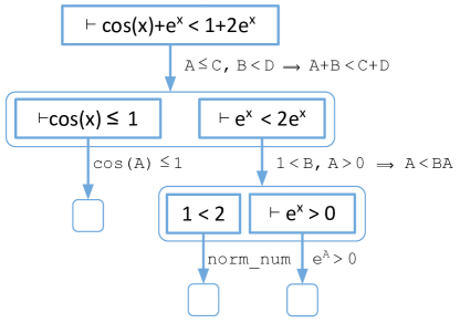
Figure 4: A visualization of the proof-tree for $\mathbf{\cos(x)+e^{x}<1+2e^{x}}$ in Equations.

4 HyperTree Proof Search

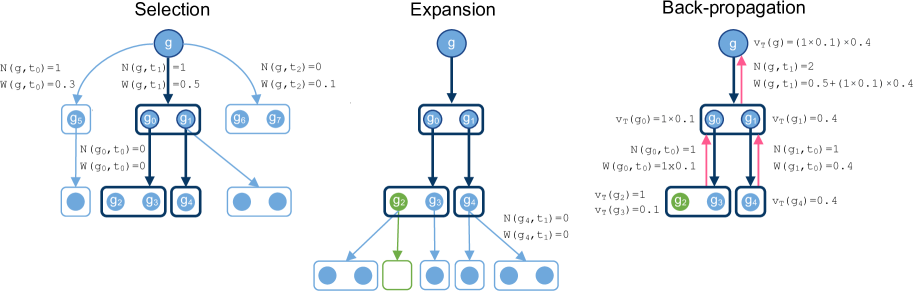
Figure 5: HyperTree Proof Search. We aim at finding a proof of the root theorem $g$ with HTPS. Proving either $\{g_{5}\}$, $\{g_{0},g_{1}\}$, or $\{g_{6},g_{7}\}$ would lead to a proof of $g$ by tactic $t_{0},t_{1}$, or $t_{2}$. The figure represents the three steps of HTPS that are repeated until a proof is found. Guided by the search policy, we select a hypertree whose leaves are unexpanded nodes. The selected nodes are then expanded, adding new tactics and nodes to the hypergraph. Finally, during back-propagation we evaluate the node values of the hypertree, starting from the leaves back to the root, and update the visit counts and total action values.

Given a main goal $g$ to automatically prove, proof search is the algorithm that interacts with our learned model and the theorem proving environment to find a proof hypertree for $g$. Proof search progressively grows a hypergraph starting from $g$. A proof is found when there exists a hypertree from the root to leaves that are empty sets.

In this section, we assume a policy model $P_{\theta}$ and critic model $c_{\theta}$. Conditioned on a goal, the policy model allows the sampling of tactics, whereas the critic model estimates our ability to find a proof for this goal. Our proof search algorithm will be guided by these two models. Additionally, and similar to MCTS, we store the visit count $N(g,t)$ (the number of times the tactic $t$ has been selected at node $g$) and the total action value $W(g,t)$ for each tactic $t$ of a goal $g$. These statistics will be used in the selection phase and accumulated during the back-propagation phase of the proof search described in Section 4.1 and Section 4.3.

The algorithm iteratively repeats the three steps described below to grow the hypergraph until either a proof is found or we exceed our expansion budget. We show an example of these three steps of proof search in Figure 5. We refer to this algorithm as HyperTree Proof Search (HTPS) throughout this work. A more detailed comparison between HTPS, MCTS, and the best-first search algorithm of Polu and Sutskever [16] can be found in Appendix A.4.

4.1 Selection

The number of nodes in the proof hypergraph grows exponentially with the distance to the root. Thus, naive breadth-first search is infeasible to find deep proofs and some prioritization criteria is required to balance depth and breadth. This is the family of best-first search algorithms, of which A* and MCTS are instances. Similar to MCTS, we balance the policy model’s prior with current estimates from the critic. In particular, we experiment with two different search policies: PUCT [33] and Regularized Policy (RP) [34], detailed in Appendix A.2. These search policies use the tactic prior from the policy model, the visit count $N$, and the estimated value of the tactic given by $Q=W/N$. A higher visit count will lead to a higher confidence in the estimated value than in the prior policy model, and vice-versa for low visit counts.

The key difference between previous work and ours is that our proof search operates on a hypergraph. Thus, whereas an algorithm like MCTS will go down a path from the root to an unexpanded node during its selection phase, our algorithm will instead create a partial proof hypertree, leading to a set of either solved or unexpanded nodes. The selection phase algorithm, described in more details in Appendix A.3, consists in recursively following the search policy from the root until we find leaves of the current hypergraph.

In Figure 5, we illustrate the selection step. We start at the root node $g$, which has three tactics $t_{0},t_{1},t_{2}$. The search policy selects $t_{2}$, leading to the set of subgoals $\{g_{0},g_{1}\}$. Then, for both $g_{0}$ and $g_{1}$, we again select the best tactic according to the search policy and finally reach the sets of unexpanded subgoals $\{g_{2},g_{3}\}$ and $\{g_{4}\}$. The final selected proof hypertree $T$ is composed of $g,\{g_{0},g_{1}\},\{g_{2},g_{3}\},\{g_{4}\}$ and is colored in dark blue in Figure 5.

In order to batch calls to the policy and critic models over more nodes to expand, we run several selections sequentially, using a virtual loss [35, 7] to produce different partial proof-trees. Note that solving all unexpanded leaves of any of these trees would immediately lead to a full proof of the root. In the next section, we describe how nodes are expanded.

4.2 Expansion

To expand a node $g$, we use the policy model to suggest tactics that would make progress on the goal, then evaluate these tactic suggestions in the theorem proving environment. Each valid tactic will lead to a set of new subgoals to solve, or to an empty set if the tactic solves the goal. Finally, we add a hyperedge for each valid tactic $t_{i}$ from the expanded node $g$ to its (potentially empty) set of children for this tactic $\{g_{i}^{0},...,g_{i}^{k}\}$. Note that these children might already be part of the hypergraph. For new nodes, visit counts $N(g,t)$ and total action values $W(g,t)$ are initialized to zero. There are three types of nodes in the hypergraph:

• Solved: at least one tactic leads to an empty set, or has all its children solved.

• Invalid: all tactics sampled from the policy model were rejected by the environment, or lead to invalid nodes.

• Unsolved: neither solved nor invalid, some tactics have unexpanded descendants.

Note that the definitions for Solved or Invalid are recursive. These status are updated throughout the hypergraph anytime a hyperedge is added. Tactics leading to invalid nodes are removed to prevent simulations from reaching infeasible nodes. Once this is done, we back-propagate values from the expanded nodes up to the root, as described in the next section.

In Figure 5, we show an example of expansion. After selecting a hypertree $T$ during the selection step, for each unexpanded leaf goal of $T$, we generate $B=2$ tactics with our policy model and keep only the valid ones. This results in two tactics for $g_{2}$ and $g_{4}$ and one for $g_{3}$. We apply these tactics in our formal environment and obtain new sets of subgoals and add them to the hypergraph. One tactic of $g_{2}$ solves $g_{2}$, resulting in an empty set of subgoals. Note that because $g_{3}$ is not solved yet, $g_{0}$ remains unsolved.

4.3 Back-propagation

For each expanded goal $g$ in a simulated proof tree $T$, its value is set to $v_{T}(g)=1$ if it is solved, and $v_{T}(g)=0$ if it is invalid. Otherwise, its value is estimated by the critic model: $v_{T}(g)=c_{\theta}(g)$. This provides $v_{T}$ for all leaves of $T$ and we can then back-propagate in topographic order (children before parents) through all nodes of $T$. Interpreting the value of a node as the probability that it can be solved, since solving a goal requires solving all of its children subgoals, the value of a parent is the product of values of its children (we assume that the solvability of subgoals is independent, for simplicity):

$$v_{T}(g)=\prod_{c\in\textrm{children}(g,t)}v_{T}(c)$$

In particular, the value of a goal $g$ is the product of the values of all leaves in $T$ that remain to be solved to obtain a proof of $g$. Once all values in $T$ are computed, we increment the corresponding visit count $N(g,t)$ in the hypergraph as well as the total action values: $W(g,t)\mathrel{+}=v_{T}(g)$. For a goal $g$, the estimated value for tactic $t$ is then the mean of the total action value:

$$Q(g,t)=\frac{W(g,t)}{N(g,t)}$$

We give an example of back-propagation in Figure 5. First, we evaluate the values of the leaf nodes of $T$. Because $g_{2}$ is solved, we set $v_{T}(g_{2})=1$. The values of $g_{3}$ and $g_{4}$ are estimated with the critic model, e.g. $v_{T}(g_{3})=c_{\theta}(g_{3})=0.1$. The values of the internal nodes are obtained by computing the product of their children values. Thus, we first compute $v_{T}(g_{0})=v_{T}(g_{2})\times v_{T}(g_{3})$ and $v_{T}(g_{1})=v_{T}(g_{4})$, then $v_{T}(g)=v_{T}(g_{0})\times v_{T}(g_{1})=(v_{T}(g_{2})\times v_{T}(g_{3}))\times(v_{T}(g_{4}))$. Then, for every (goal, tactic) pair $(g,t)$ in $T$, we increment the visit count, $N(g,t)\mathrel{+}=1$ and update the total action value: $W(g,t)\mathrel{+}=v_{T}(g)$.

5 Online training from proof searches

In the previous section, we considered the policy and critic models as given. In this section, we explain how proof search is used to create training data for these two models. Provers are asynchronously running proof searches using a version of the models synchronized with the trainers, coupling training and data extraction in an online procedure that leads to continuous performance improvements.

5.1 Training objectives

Both the policy model $P_{\theta}$ and the critic model $c_{\theta}$ are encoder-decoder transformers [36] with shared weights $\theta$, which are trained with a tactic objective and a critic objective respectively.

Tactic objective.

The policy model $P_{\theta}$ takes as input a tokenized goal and generates tactics. It is trained with a standard seq2seq objective [24], where we minimize the cross-entropy loss of predicted tactic tokens conditioned on an input goal.

Critic objective.

In order to decode a floating point value with our seq2seq critic model $c_{\theta}$, we start decoding with a special token, restrict the output vocabulary to the two tokens PROVABLE and UNPROVABLE, and evaluate the critic with $c_{\theta}(g)=P(\texttt{PROVABLE}|g,\texttt{CRITIC})$. The critic objective is identical to a seq2seq objective where the cross-entropy is minimized over the two special tokens.

5.2 Online training

We use a distributed learning architecture reminiscent of AlphaZero [33] or distributed reinforcement learning setups [37, 7]. A distributed data parallel trainer receives training data from a set of asynchronous provers that run proof searches on tasks chosen by a controller that also centralizes statistics. Provers, in turn, continuously retrieve the latest model versions produced by the trainers in order to improve the quality of their proof search. This set-up is represented in Figure 6. Once a prover finishes a proof-search, we extract two types of training samples from its hypergraph:

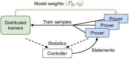
Figure 6: An overview of our online training architecture. The controller sends statements to asynchronous HTPS provers and gathers training and proving statistics. The provers send training samples to the distributed trainers and periodically synchronize their copy of the models.

Tactic samples.

At the end of a successful proof search, we extract (goal, tactic) pairs of a minimal proof hypertree of the root node as training samples for the policy model. This selection has a large impact on performances, other options such as selecting all solved nodes are investigated in Section 7.2.1. We use a different minimality criteria depending on the environment: total number of proof steps for Metamath and Equations, and total tactic CPU time for Lean (see Appendix E for details).

Critic samples.

In the proof search hypergraph, we select all nodes that are either solved, invalid, or with a visit count higher than a threshold. Then, we use $c(g)=1$ as the training target for solved nodes. For internal nodes, we use the final estimated action value $c(g)=W(g,t^{*})/N(g,t^{*})$ where $t^{*}$ is the tactic that maximizes the search policy at $g$. Finally, for invalid nodes, we use $c(g)=0$.

The trainers receive training samples that are stored into two separate finite-size queues, one for each objective. When a queue is full, appending a new sample discards the oldest one. In order to create a batch for a task, we uniformly select samples in the corresponding queue. The two training objectives are weighted equally. Additionally, during online training, we continue sampling from the supervised tasks which provide high-quality data.

Our proof-search depends on many hyper-parameters, and the optimal settings might not be the same for all statements, making tuning impractical. Thus, the controller samples these hyper-parameters from pre-defined ranges (see Appendix C for details) for each different proof-search attempt.

5.3 Full training pipeline

In order to bootstrap our online learning procedure we require a policy model $P_{\theta}$ that outputs coherent tactics. While the critic is left untrained, the policy model is fine-tuned on a pretrained transformer using a supervised dataset specific to the target environment. Overall, the full training pipeline can be summarized as follows:

• Pretraining of the encoder-decoder model on a large unsupervised corpus (c.f. Section 6.2).

• Fine-tuning of the policy model on supervised datasets detailed in (c.f. Section 6.1).

• Online training of both the policy and critic models on data extracted from proof search.

6 Experiments

In this section, we provide details about our experimental training and evaluation protocols. We first describe the supervised datasets used to fine-tune our policy models, as well as the tokenization used. We then give practical details on pretraining and the model architecture. Finally, we discuss the evaluation datasets and methodology.

6.1 Model fine-tuning and supervised datasets

Starting the HTPS procedure described in Section 5 from a randomly initialized model would be sub-optimal, as no valid tactic would ever be sampled from the policy model. Thus, starting the online training from a non-trivial model is critical. To this end, we first fine-tune our policy model $P_{\theta}$ on a supervised dataset of theorems specific to each environment.

Metamath

In Metamath, we extract all proofs from the set.mm library, composed of 37091 theorems (c.f. Section D for the version of set.mm). We first derive a graph of dependencies between statements, and generate a random train-valid-test split of theorems, with 1000 valid and test theorems. We use the DAG to ensure that each theorem in the valid or test set is not used to prove another theorem. Moreover, this DAG is used to build a table of forbidden tokens: if the proof of $A$ depends on $B$, we set to zero the probability of generating the token $A$ during a proof-search of $B$. We use a seq2seq training objective, where the model is conditioned on a goal to prove, and is trained to output a sequence of the following format:

LABEL MANDATORY_SUBSTS <EOU> LABEL_STATEMENT PREDICTABLE_SUBSTS <EOS>

LABEL is the label of the rule to apply, MANDATORY_SUBSTS is a serialized version of the substitutions in the rule that cannot be inferred from syntactic parsing of the input goal and the theorem statement. During proof-search, decoding is stopped at the <EOU> (End Of Useful) token and we do not generate predictable substitutions, as this would unnecessarily increase decoding time and the probability that our model generates invalid substitutions. Training the model to output predictable substitutions and the rule statement serves as a co-training task and helps reduce overfitting. The training set is composed of around 1M goal-tactic pairs; more statistics about the training data are provided in Table 1. Tokenization in Metamath is trivial, as statements are composed of space-separated tokens.

	# train theorems	# train proof steps	Avg. goal length
Equations	$\infty$	$\infty$	33.7
Metamath	35k	1M	120.1
Lean	24k	144k	169.3

Table 1: Dataset statistics for supervised training.

Lean

Following [18], we extract a supervised dataset from the Mathlib library. The training set is composed of 24k theorems and 144k goal-tactic pairs. In addition, we co-train with the dataset of proof-artifacts of Han et al. [17] to reduce overfitting. To facilitate experimentation and reproducibility, we use fixed versions of Lean, Mathlib, and miniF2F (c.f. Appendix D). Finally, we add another supervised co-training task by converting to Lean a synthetic dataset of theorems generated by the Equations environment (c.f. Appendix B.7). In order to avoid hooking into the Lean parser, we tokenize goals and tactics using byte-pair encoding (BPE [38]) following previous work [16, 18]. Statistics about the training set are available in Table 1.

Equations

Unlike Metamath or Lean, the Equations environment does not come with with a dataset of manually annotated proofs of theorems. Instead, we generate supervised data on the fly using the random graph generator described in Appendix B.6. As the model quickly reaches a 100% proving accuracy on these synthetic theorems, there would be no benefit in using them during online training. Thus, we fine-tune on the synthetic dataset, and only leverage statements from the Identities split during online training. As in Metamath, tokenization of statements for this environment is natural, as each statement can be tokenized using the list of symbols from its prefix decomposition [27].

6.2 Model pretraining

Model pretraining can be critical in low-resource scenarios where the amount of supervised data is limited [39, 40]. Thus, we do not immediately fine-tune our model but first pretrain it on a large dataset to reduce overfitting and improve generalization. In particular, we pretrain our model with a masked seq2seq objective (MASS [41]) on the LaTeX source code of papers from the mathematical section of arXiv. After tokenization, our filtered arXiv dataset contains around 6 billion tokens for 40GB of data. Similar to Polu and Sutskever [16], we observed large performance gains using pretraining. However, we found that arXiv alone provides a better pretraining than when it is combined with other sources of data (e.g. GitHub, Math StackExchange, or CommonCrawl).

6.3 Model Architecture and Training

Model architecture.

Our transformer architecture uses a 12-layer encoder and a 6-layer decoder in all experiments. We use an embedding dimension of 1600 in the encoder and 1024 in the decoder for both Metamath and Lean. For Equations, where we expect the model to require less decoding capacity, the decoding dimension is lowered to 512. We found that reducing the decoder capacity increases the decoding speed without impacting the performance, as previously observed by Kasai et al. [42] in the context of machine translation. Our models are composed of 440M parameters for Equations and 600M parameters for Metamath and Lean (for comparison, GPT-f uses a 770M parameter, 36-layer model).

Supervised fine-tuning.

During fine-tuning, we train our models with the Adam optimizer [43] and an inverse square-root learning rate scheduler [36]. We use a dropout of 0.2 [44] to reduce the overfitting of our models. We also apply layer-dropout [45] with a dropout rate of 0.1 to further reduce overfitting and stabilize training. We implement our models in PyTorch [46] and use float16 operations to speed up training and to reduce the memory usage of our models.

Online training.

During online training, we alternate between the goal-tactic objective, used during fine-tuning on the supervised dataset, and the goal-tactic and goal-critic objectives on data generated by the provers. As the model and the data generated by the provers are constantly evolving, we do not want the learning rate to decrease to 0, and we fix it to $3\times 10^{-5}$ after the warm-up phase. Unless mentioned otherwise (e.g. for large experiments), we run all Metamath and Equations experiments with 16 trainers and 32 provers for a total of 48 V100 GPUs.

6.4 Evaluation settings and protocol

In Polu et al. [18], the model is fine-tuned on theorems from the training set and expert iteration is done on theorems from different sources: train theorems, synthetic statements, and an extra curriculum of statements without proofs (miniF2F-curriculum). The produced model is then evaluated on unseen statements, namely the validation and test splits of the miniF2F dataset [8].

In this work, we also consider the transductive setup: on a corpus of unproved statements available at train time, how many proofs can our method learn to generate? This protocol is also sensible, as allowing the model to learn from a failed proof-search can lead to more focused exploration on the next attempt, proving more statements overall than a model that would not be trained online.

Following [16], we also evaluate the pass@k by running $k$ proof searches on the evaluated statements with the policy and critic obtained by online training. In the transductive setup, we also report the cumulative pass rate, i.e. the proportion of theorems solved at least once during online training.

7 Results

In this section, we present our results and study the moving parts of our pipeline through ablations. Each experiment is run on a single environment (e.g. Lean, Metamath, or Equations). We compare our model with GPT-f[16, 17, 18] which represents the state of the art on Metamath and Lean.

7.1 Main Results

	Supervised	GPT-f	Evariste-1d	Evariste-7d	Evariste
Online training statements	-	miniF2F-curriculum			miniF2F-valid
miniF2F-valid	38.5	47.3	46.7	47.5	58.6†
miniF2F-test	35.3	36.6	38.9	40.6	41.0
miniF2F-curriculum	20.8	30.6	33.6†	42.5†	32.1
Train time (A100 days)	50	2000	230	1620	1360

Table 2: Pass rate on Lean environment using 64 trials (pass@64). Numbers with a ^† exponent correspond to the cumulative pass-rate since the evaluated statements are part of the online training. Evariste refers to the method described in this paper.

7.1.1 Lean

In Lean, we run our experiments on A100 GPUs with 32 trainers and 200 provers. Each prover runs our Lean API on 48 CPU cores. Unlike Polu et al. [18], we sample statements equally from mathlib-train and miniF2F-curriculum, to avoid giving too much importance to statements from a different domain than the target. After 1 day of training (i.e. $(200+32)$ A100 days of compute), each statement from miniF2F-curriculum has been sampled on average $250$ times, and $110$ out of the $327$ statements have been solved. Our model outperforms GPT-f on miniF2F-test, with an approximately $10\times$ training time speed-up. After $7$ days, we solve $139$ statements of miniF2F-curriculum ($100$ for GPT-f), and observe further improvements on miniF2F-valid or miniF2F-test.

For other evaluations, we depart from the set-up of Polu et al. [18], directly using the statements from the miniF2F-valid split in our online training, obtaining 58.6% cumulative pass rate. We then evaluate the final model on miniF2F-test, reaching 41% pass@64, against 36.6% for GPT-f.

Without the synthetic data co-training task, the performance drops to $54.9\%$ cumulative pass rate on the miniF2F-valid split, and $38.5\%$ pass@64 on the miniF2F-test split. Examples of proofs found by our model can be found in Appendix F.

7.1.2 Metamath

On Metamath, we train our model on V100 GPUs, with 128 trainers and 256 provers, whereas ablations are run on 16 trainers and 32 provers. We report our results in Table 3 for the supervised model and for a model trained with online training. During online training, we sample equally statements from the training and from the validation splits of set.mm.

Online training dramatically improves performances on valid statements, going from a $61\%$ pass@8 to a cumulative pass rate of $82.6\%$ on this split. This improvement cannot solely be explained by the high number of attempts on validation theorems during training. Indeed, the ablation in Figure 7 (right) shows that Evariste significantly outperforms a supervised model with the same number of attempts. The supervised model plateaus at $66\%$ while Evariste keeps improving beyond $74\%$ after 7 days of training, showing that the model is able to learn from previous proof searches through online training.

On test theorems, for which statements were not provided during online training, the pass@32 accuracy increased by $10\%$ compared to the supervised model, from $55.8\%$ to $65.6\%$. Note that the supervised model already obtains an accuracy of $65.4\%$ (resp. $61.2\%$) on the validation (resp. test) split, compared to GPT-f’s $56.5\%$ (resp. $56.2\%$) after expert iteration, showing the benefits of HTPS.

	Valid			Test
	cumulative	pass@8	pass@32	pass@8	pass@32
Supervised	N/A	61.0%	65.4%	55.8%	61.2%
Evariste	82.6%	81.0%	81.2%	65.6%	72.4%

Table 3: Results on Metamath for a supervised model and Evariste. We report the pass@8 and pass@32 scores on the validation and test splits. Additionally, for Evariste we also report the cumulative score on the validation set, i.e. the fraction of theorems proved at least one time during online training. Note that for Evariste on Valid, the cumulative and pass@k performances are close since these statements were seen during training.

7.1.3 Equations

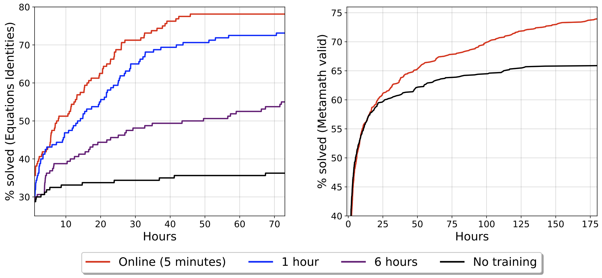
Figure 7: Comparison between online setup, expert iteration, and fixed model. We report the cumulative pass rate on the Identities (resp. valid) split for the Equations (resp. Metamath) environment. Reloading the model more frequently converges faster and to a better performance. When “No training” is done (i.e. the model is the supervised one), the final performance is much lower despite using as many attempts. This shows that online training is able to learn from previous proof searches.

In Equations, we run our main experiment with 32 trainers and 64 provers, whereas ablations are run on 16 trainers and 32 provers. In this environment, the model easily learns the training distribution of our random generator, and solves all synthetically generated problems. Thus, online training is run on the Identities statements only. Our main experiment reaches a cumulative pass rate of $91.3\%$ on the Identities split, while a supervised model never exceeds $36\%$ even after a similar number of proof attempts. In Appendix 9, we give examples of Identities statements proved during online training, as well as the size and depth of proofs found by the model.

In particular, Evariste managed to find the proof of complex mathematical statements, such as $\sinh(x/2)=\sinh(x)/\sqrt{2(1+\cosh(x))}$ and $\tan(3x)(1-3(\tan(x))^{2})=3\tan(x)-(\tan(x))^{2}\tan(x)$ that required 82 and 117 proof steps respectively, showing the abilities of HTPS to prioritize subgoals and guide the search in very large proof graphs. This shows that online training is able to adapt our policy and critic models to a completely new domain, going from automatically generated statements to identities found in math books. Examples to understand the gap between these two domains can be found in Appendix B.

7.2 Ablation study

In this section, we present an ablation study on several components of our system. Since Lean experiments are CPU intensive, we run most of our ablations on the Equations and Metamath environments. On Lean, we ran experiments on a smaller subset of hyper-parameters that consistently performed well on the other environments.

7.2.1 Online training data for tactic objective

Proof Of	All Solved		Root		All Nodes
Type of Proof	All	Min	All	Min	-
Metamath (valid)	61.2	65	57.4	68.6	51.6
Metamath (test)	57.2	58.8	54.8	57.4	54.4
Equations (Identities)	40.6	78.1	37.5	71.3	37.5

Table 4: Performance of our model for different online training data for tactic objective We report the pass@8 score for Metamath and cumulative pass rate for Equations. We try to keep all nodes and sample the tactics of these nodes according to the policy. We also try to extract proofs or minimal proofs of solved nodes, or the proofs or minimal proofs of the root theorem only. Selecting minimal proofs always improves performances and gives the best results in both environments.

The way we filter tactics sent to the trainers has a large impact on final performances. We investigated several filtering methods and report the results in Table 4. The first method is similar to the one used in AlphaZero and exposed in [33]: we select all nodes of the proof search hypergraph where the visit count is above a certain threshold and we filter tactics above a given search policy score. At training time, tactics are sampled according to the filtered search policy. With this method the model reaches 51.6% pass@8 on the valid set of Metamath and 37.5% cumulative pass rate on Equations.

We then experimented with other filtering criteria, selecting only goal-tactic pairs that are part of proofs: either a proof of the root node, or of any solved node in the hypergraph. Then, we learn from all possible proofs, or only from proofs that are minimal according to a criteria (number of proof steps for Equations and Metamath, cumulative CPU time for Lean).

Learning only from the minimal proofs always leads to improved performance, regardless of the selected roots. Learning from the minimal proofs of all solved nodes, we reach a cumulative pass rate of 78.1% on Equations, compared to 40.6% when learning from all proofs. On Metamath, only learning from the root’s minimal proof gives the best result on the validation set, reaching a pass@8 of 68.6%.

7.2.2 Critic

	Evariste	No critic	Hard critic	Fixed search params
Metamath (valid)	68.6	64.8	67.6	69.8
Metamath (test)	57.4	52.2	57.4	56.2
Equations (Identities)	78.1	65.6	63.1	73.8

Table 5: Ablation study on the critic and search hyper-parameters in HTPS. We report the pass@8 score for Metamath, and the cumulative pass rate for Equations. Evariste, trained with a soft critic and stochastic hyper-parameters, obtains the best performance in both environments. Removing the critic, or using a hard critic (e.g. when the critic is trained to predict 1 on solved nodes and 0 on others) leads to reduced performances. In Equations, adding stochasticity in the proof search hyper-parameters increases the performance by $4.3\%$ in Equations, and slightly improves performance in Metamath.

To measure the impact of our critic model, we run an experiment where the proof search is only guided by the policy model. During the back-propagation phase, we set $v_{T}(g)$ to $0.5$ for the leaves of $T$. In that context, our model is no longer trained with a critic objective. We run this experiment for both Equations and Metamath, and report the results in Table 5. In both environments, using a critic model improved the performance significantly, by $5.2\%$ and $12.5\%$ on Metamath and Equations respectively.

As mentioned in Section 5, to train the critic objective, we set the training targets as $c(g)=1$ for solved nodes, $c(g)=0$ for invalid nodes and $c(g)=W(g,t^{*})/N(g,t^{*})$ where $t^{*}$ is the tactic that maximizes the search policy at $g$., for internal nodes. We also tested a hard critic estimation of the target values, following Polu and Sutskever [16], where $c(g)=1$ for solved nodes and $c(g)=0$ for both invalid and internal nodes. We report results in Table 5. For both Metamath and Equations, estimating the critic target of internal nodes with the HTPS action value estimate allows Evariste to reach its best performance. In Equations, the model reaches a cumulative pass rate of 78.1%, compared to 63.1% with hard critic estimates. In Equations, using hard critic targets gives worse performances than having no critic model at all, showing that these targets are a bad estimation: setting all internal nodes to zero is too pessimistic.

7.2.3 Fixed proof search parameters

We study the impact of sampling HTPS hyper-parameters for each attempt during online training. We run experiments with fixed, chosen search parameters for Equations and Metamath to compare with random sampling, and report results in Table 5. Evariste achieves better performances than the model trained with fixed search parameters on Metamath test set and Equations Identities, reaching 78.1% pass rate compared to 73.8% in Equations Identities.

7.2.4 Model update frequency during online training

In our online training procedure, the policy and critic models are updated every five minutes on the provers. We measure the impact of the frequency of these updates by trying different refresh rates: 5 minutes, 1 hour, 6 hours for Equations, and no updates at all for both Equations and Metamath. We report the cumulative pass rate over training hours in Figure 7. The higher the refresh rate, the better the cumulative pass rate over time, confirming the benefits of online training over expert iteration.

8 Conclusion

In this work, we introduce HTPS, an AlphaZero-inspired proof search algorithm for automated theorem proving, along with an online training procedure. We run an extensive study of our pipeline, and present state-of-the-art results on multiple proving environments. We show that online training provides large speed-ups over expert iteration, and allows generalization of the policy and critic models to completely new domains. Despite large number of attempts per theorem, proving the entirety of datasets like miniF2F remains elusive, and generating data from proof-search on the currently available corpora will likely be insufficient in the long term. As manually annotated formal datasets are limited, another way of providing exploration and additional training data (in the spirit of self-play for two player games) is required. Automated generation of new theorems is likely to be one of the future milestones.

Acknowledgments

We thank the Meta AI and FLARE teams for useful comments and discussions throughout this work, notably, Faisal Azhar, Antoine Bordes, Quentin Carbonneaux, Maxime Darrin, Alexander Miller, Vincent Siles, Joe Spisak and Pierre-Yves Strub. We also thank the members of the Lean community for their help, notably Fabian Glöckle for valuable feedback on this project.

Appendix A Proof search in more details

A.1 Hypergraph and definitions

We begin with some useful notations and concepts for our hypergraphs.

Formally, let $\mathcal{G}$ be a set of nodes, and $\mathcal{T}$ a set of tactics. A hypergraph is a tuple $H=(G,r,T,U)$ with $G\subset\mathcal{G}$ the nodes, $r\in G$ the root, and $T\subset G\times\mathcal{T}\times\mathcal{P}(G)$ the admissible tactics. An element of $T$ is written $(g,t,c)$ where $g$ is the start goal, $t$ is the applied tactic and $c$ is the potentially empty set of children that the tactic creates when applied to $g$ in the proving environment.

A hypertree is a hypergraph without cycles, i.e, such that we cannot find a path $g_{0},\dots,g_{\ell}=g_{0}$ with $\ell>0$ and with $g_{i+1}$ in the children of $g_{i}$ for all $i$’s.

Let $S\subset G$ be the set of solved nodes. A node $g\in G\setminus U$ is solved if one of its tactic leads to no subgoals, or one of its tactics leads to only solved nodes. Formally: $\exists(g,t,\emptyset)\in T$ or $\exists(g,t,c)\in T$ such that $c\subset S$. We say that a tactic $t$ is solving for $g$ if all the children it leads to are solved. Conversely, let $U\subset G$ be the set of invalid nodes. A node $g\in G\setminus U$ is invalid if it has been expanded but has no tactics in the hypergraph, or all of its tactics have an invalid child. Formally: $\{(g,t,c)\in T\}=\emptyset$ or $\forall(g,t,c)\in T$, $c\cap I\neq\emptyset$.

These recursive definitions naturally lead to algorithms MaintainSolved and MaintainStatus to maintain sets $S$ and $I$ when elements are added to $H$.

A sub-hypertree $H_{T}$ of $H$ is a connected hypertree rooted at some goal of $H$. Its leaves $\textrm{leaves}(H_{T})$ are its subgoals without children (either elements of $U$ or $S$). The set of proofs of $g$ in $H$, $\textrm{Proofs}(g,H)$ are all the hypertrees rooted at $g$ that have all their leaves in $S$. Similarly, the expandable subtrees of $H$ rooted in $g$, $\textrm{Expandable}(g,H)$ are the subtrees with at least one leaf in $U$. A tactic is said to be expandable if it is part of an expandable subtree, this can be computed with a graph-search ComputeExpandable.

We can now reformulate the process of proof-search. Starting from a hypergraph that contains only the root theorem $r$, we produce a sequence of expandable subtrees. The unexpanded leaves of these subtrees are expanded in the hypergraph, then the new value estimates are backed-up. The hypergraph grows until we use all our expansion budget, or we find a proof of $r$.

A.2 Policies

When a goal $g$ is added to the hypergraph, its visit count $N(g,t)$ and total action value $W(g,t)$ are initialized to zero. Its virtual visit count $VC(g,t)$ are updated during proof search. Let $C(g,t)=N(g,t)+VC(g,t)$ be the total counts. These values are used to define the value estimate with a constant first play urgency [47]:

$$Q(g,t)=\left\{\begin{array}[]{ll}\frac{\max(1,N(g,t))}{\max(1,C(g,t))}&\mbox{if $t$ is solving for $g$}\\ \frac{0.5}{\max(1,C(g,t))}&\mbox{if }N(g,t)=0\\ \frac{W(g,t)}{C(g,t)}&\mbox{otherwise.}\end{array}\right.$$

Notice that the value of solving tactics decreases with virtual counts, allowing exploration of already solved subtrees.

Given the visit count $N$, the total counts $C$, value estimates $Q$, the model prior $P_{\theta}$ and an exploration constant $c$. The policy used in Alpha-Zero is PUCT:

$$\textrm{PUCT}(g)=\textrm{arg}\max_{t\in\mathcal{A}}\left[Q(g,t)+c\cdot P_{\theta}(t|g)\cdot\frac{\sqrt{\sum N(g,\cdot)}}{1+C(g,t)}\right]$$

Notice that more weight is given to the value estimate $Q$ as $N$ grows which decreases the second term. Another work [34] obtains good performances using as search policy the greedy policy regularized by the prior policy.

$$\pi_{RP}(g)=\textrm{arg}\max_{y\in\mathcal{S}}\left[Q(g)^{T}y-c\cdot\frac{\sqrt{\sum C(g,\cdot)}}{\sum(C(g,\cdot)+1)}KL(\pi_{\theta},y)\right]\quad{\textrm{with $\mathcal{S}$ the policy simplex at $g$}}$$

Again, note that this policy balances the prior with the value estimates as the count grows, but does not account for individual disparities of visits of each tactics. In our experiments, we obtained better performances with $\pi_{RP}$ on Equations, and better performances with $PUCT$ on Metamath and Lean.

A.3 Algorithms

Simulation

During simulation, we only consider subtrees that could become proofs once expanded. This means we cannot consider any invalid nodes or consider subgraphs containing cycles. If we encounter a tactic that creates a cycle during a simulation, this tactic is removed from the hypergraph, virtual counts from this simulation are removed and we restart the search from the root. This may remove some valid proofs, but does not require a backup through the entire partial subtree which would lead to underestimating the value of all ancestors. Removing tactics from the hypergraph also invalidates computations of expandable tactics. This is dealt with by periodically calling MaintainExpandable if no valid simulation can be found. A full description of the algorithm that finds one expandable subtree is available in Algorithm 1. Selection of nodes to expand requires finding expandable subtrees until a maximum number of simulations is reached, or no expandable tactic exists at the root.

Algorithm 1 Finding an expandable subtree

  Input: A hypergraph $H$ and its $root$

  Output: A partial proof tree with unexpanded leaves

  :start

  T: hypertree($root$)

  to_explore: list = [$root$]

  while to_explore do

     g = to_explore.pop()

     if g is internal then

        if $\textrm{expandable}(g)\neq\emptyset$ then

           tactic = $\textrm{arg}\max_{t}{\left.\kern-1.2pt\pi\vphantom{\big{|}}\right|_{\textrm{expandable}(g)}}\pi(g,t)$

        else

           continue { expandable nodes are in a sibling branch }

        end if

        if tactic leads to cycle then

           kill tactic

           remove virtual counts for elements of T

           goto start

        end if

        $VC(g,tactic)\mathrel{+}=1$

        T.add(g, tactic, children(g, tactic))

        to_explore += [children(g, tactic)]

     end if

  end while

Expansion

The policy model produces tactics for an unexpanded node $g$. These tactics are evaluated in the proving environments. Valid tactics are filtered to keep a unique tactic (e.g. the fastest in Lean) among those leading to the same set of children. Finally, we add the filtered tactics and their children to the hypergraph. If no tactics are valid, the node is marked as invalid and we call MaintainInvalid. If a tactic solves $g$, the node is marked as solved and we call MaintainSolved.

Backup

The backup follows topological order from the leaves of a simulated partial proof-tree $T$, updates $W$ and $N$, and removes the added virtual count. The algorithm is described in Algorithm 2

Algorithm 2 Back-propagation of total action value $W$

  Input: Partial proof-tree $T$ and value estimates $c_{\theta}(g)$ of its leaves.

  to_backup = []

  for $g$ in leaves of T do

     $v_{T}(g)=c_{\theta}(g)$

     to_backup.append($\textrm{parent}_{T}(g)$)

  end for

  while to_backup do

     $g$ = to_backup.pop()

     to_update = $\prod_{c\in\textrm{children}_{T}(g)}$ $v_{T}(c)$

     $W(g,t)\mathrel{+}=$ to_update

     $N(g,t)\mathrel{+}=1$

     $VC(g,t)\mathrel{-}=1$

     $v(g,t)=$ to_update

     $g$.is_prop = true

     if all $c$.is_prop for $c$ in $\textrm{siblings}_{T}(g)$ then

        to_backup.append($\textrm{parent}_{T}(g)$)

     end if

  end while

A.4 Comparison with other search algorithms

Best First Search [16].

This best-first search expands goals one at a time according to a priority-queue of either a value model or the cumulative log-prior from the language model. Since the priority is equal among siblings but strictly decreasing with depth, this means siblings will always be expanded together. However, nothing prevents the algorithm from jumping from one potential proof-tree to another, and potentially favoring breadth over depth. In comparison, depth does not appear in the value estimate we compute, but rather the remaining number of nodes to solve a particular proof-tree. Moreover, our algorithm leads to value estimates that can be used to train our critic, which performs better than 0-1 estimates provided by best-first search (c.f. Section 7.2.2).

Monte Carlo Tree Search [6].

MCTS has been famously used as part of AlphaZero [33] to obtain great performances on two player games. This two player set-up can be mapped to theorem-proving by assigning one player to choosing the best tactics while the other player picks the most difficult goal to solve (a method explored in Holophrasm [19]). However, since we need to provide a proof of the root theorem, we need to ensure that we can solve all goals that a tactic leads to. This set-up has been studied for two player games when attempting to compute the game-theoretical value of positions. Using MCTS in this set-up is suboptimal [48], ignoring unlikely but critical moves from the opponent (in our case, a subgoal that looks easy but is impossible to solve). We decided to exploit the highly asymmetrical arities of our two players (most tactics lead to one or two goals) which makes simulating partial proof-trees computationally feasible. Thus, the values we back-propagate always take into account all possible moves from the opponent, while only requiring a few expansions per simulation.

Appendix B Equations environment

In this section, we give additional details about the environment Equations. First, we described its main elements, theorems (resp. tactics) in Section B.1 (resp. B.2). Then, we describe a proof in this environment in Section B.3, how numerical expressions are evaluated in Section B.4 and what vulnerabilities this can lead to in Section B.5. Finally, we describe our random theorem generator in Section B.6 and how theorems and their proofs can be translated to Lean in Section B.7.

B.1 Theorems

Each theorem in Equations consists in proving mathematical expressions composed of functions of real numbers, by manipulating and rewriting expressions. A theorem to prove can be an inequality or an equality, conditioned to a set (potentially empty) of initial assumptions. For instance:

$$x^{2}+1\geq 2x\;\;\;\;\textrm{or}\;\;\;\;x>y\implies e^{y-x}-1<0$$

In the first example, the goal does not have any hypothesis and consists in proving that for every $x\in\mathbb{R}$, $x^{2}+1\geq 2x$. In the second example, the goal consists in proving that $e^{y-x}-1<0$ for every $x,y\in\mathbb{R}$ that satisfy the hypothesis $x>y$.

Equalities and inequalities are represented as trees with the three following elements:

• Leaves: represent a variable, an integer, or a constant (e.g. $\pi$).

• Internal nodes: represent unary or binary operators, e.g. $+$, $-$, $/$, $\times$, $\exp$, $\ln$, $\cos$, $\sin$, $\sinh$, $\cosh$, etc. More advanced operators such as $\gcd$, $\mathrm{lcm}$, $\mathrm{mod}$ (the rest of an euclidean division) are possible when dealing with integers.

• A root node: represents a comparison operator, e.g. $=$, $\leq$, $<$, $\geq$, $>$, $\neq$. More advanced comparison operators such as $|$ (divides) are possible when dealing with integers.

B.2 Tactics

Equations allows to deduce equalities and inequalities from simpler subgoals, using elementary rules (i.e. tactics). The environment contains two types of rules: transformations, which consist in matching a pattern in an expression and replacing it by an equivalent expression; and assertions, which consist in asserting that an expression is true. Both types of rules can have assumptions.

Transformation rules

A transformation rule (TRule) consists in a set of two expressions, $L$ and $R$, equivalent under a set of assumptions $S$. For instance $\texttt{TRule}(A+B,B+A)$ is the transformation rule stating the commutativity of the addition, namely that $A+B=B+A$ for any expressions $A$ and $B$. Note that in this case, the set of assumption $S$ is empty as the equality always holds. Another example is $\texttt{TRule}(\sqrt{A^{2}},A,[A\geq 0])$ that states that $\sqrt{A^{2}}=A$ provided that $A\geq 0$.

Applying such a rule to an existing equation works as follows:

• matching a term $T$ in the expression that has the pattern of $L$

• identifying the matching variables and substituting them in $R$

• replacing $T$ by R in the input equation

• return the resulting equation with the set of hypotheses required for the transformation

For instance, if the input goal is:

$$\sqrt{({e^{x}})^{2}}=e^{x}$$

Applying $\texttt{TRule}(\sqrt{A^{2}},A,[A\geq 0])$ on this expression will result in two subgoals:

• The same expression, where $\sqrt{A^{2}}$ has been replaced by $A$: $e^{x}=e^{x}$

• The hypothesis required for the assumption to hold: $e^{x}\geq 0$

More generally, a transformation rule will result in $N+1$ subgoals, where $N$ is the number of hypotheses required by the rule.

Assertion rules

An assertion rule (ARule) expresses the fact that an expression is true, provided some hypotheses. It is represented by a main expression, and a set of assumptions sufficient for the main expression to hold. For instance, the rule $\texttt{ARule}(A\leq C,[A\leq B,B\leq C])$ states the transitivity of the partial order $\leq$, i.e. $A\leq C$ provided that there exists an expression $B$ such that $A\leq B$ and $B\leq C$.

Assertion rules do not always have hypotheses, for instance the reflexivity rule $\texttt{ARule}(A=A)$, or the rule $\texttt{ARule}(e^{A}>0)$ stating that $e^{A}$ is positive, for any real value $A$. Note that the two subgoals generated in the previous paragraph ($e^{x}=e^{x}$ and $e^{x}>0$) can be respectively solved by these two assertion rules (i.e. by matching $A=e^{x}$ and $A=x$).

Unlike transformation rules that always result in at least one subgoal (the initial expression on which we applied the transformation), assertion rules will only generate $N$ subgoals, where $N$ is the number of hypotheses. As a result, being able to apply an assertion rule without hypotheses to an expression is enough to close (e.g. solve) the goal. Assertion rules are in fact very similar to rules in Metamath.

In Table 6, we provide the number of Equations rules in different categories. Some examples of transformation and assertion rules are given in Table 7.

Rule type	Basic	Exponential	Trigonometry	Hyperbolic	All
Transformation	74	18	9	8	109
Assertion	90	11	9	0	110
Total	171	29	18	11	219

Table 6: Number of Equations rules in each category.

Transformation rules	Assertion rules
$\sin(0)=0$	$|\cos(A)|\leq 1$
$\cos(0)=1$	$|\sin(A)|\leq 1$
$\sin(\frac{\pi}{2})=1$	$|\sin(A)|\leq|A|$
$\cos(\frac{\pi}{2})=0$	$A=B\implies\sin(A)=\sin(B)$
$\sin(-A)=-\sin(A)$	$A=B\implies\cos(A)=\cos(B)$
$\cos(-A)=\cos(A)$	$\sin(A)\neq\sin(B)\implies A\neq B$
$\cos(A)\neq 0\implies\tan(A)=\frac{\sin(A)}{\cos(A)}$	$\cos(A)\neq\cos(B)\implies A\neq B$
$\sin(A+B)=\sin(B)\cos(A)+\sin(A)\cos(B)$	$A=B,\cos(A)\neq 0\implies\tan(A)=\tan(B)$
$\cos(A+B)=\cos(A)\cos(B)-\sin(A)\sin(B)$	$\tan(A)\neq\tan(B),\cos(A)\cos(B)\neq 0\implies A\neq B$

Table 7: Trigonometric rules accessible by the model. The model only has access to these elementary rules when proving statements from Identities. In particular, it cannot use more involved theorems such as $\cos^{2}(x)+\sin^{2}(x)=1$ or $\sin(\pi)=0$.

B.3 Proving a statement with Equations

In order to prove a theorem with Equations, the user (or automated prover) has to apply tactics on the current expression. A tactic can correspond either to a transformation rule, or to an assertion rule.

For transformation rules, the model needs to provide:

• the rule (using a token identifier)

• the direction in which the rule is applied (a Boolean symbol, for forward or backward)

• an integer that represents the position where the rule is applied

• an optional list of variables to specify (c.f. paragraph below)

The direction of the rule indicates whether we want to transform $L$ by $R$ or $R$ by $L$ (e.g. replace $A$ by $\sqrt{A^{2}}$, or the opposite). The position where the rule is applied is given by the prefix decomposition of the input expression. For instance, the prefix notation of $(x+y)+1$ is given by + + x y 1. Applying the commutativity rule $A+B=B+A$ to the expression in position 0 will result in $1+(x+y)$. Applying it in position 1 will result in $(y+x)+1$, since the rule was applied to $(x+y)$. Note that for the commutativity rule, the direction in which we apply the rule does not matter. The list of variables to specify is required when variables in the target patterns are absent from the source pattern. For instance, applying the transformation rule TRule(A,A+B-B) in the forward direction will require to provide the value of $B$.

For assertion rules, the format is simpler. We no longer need to specify a direction or a position (the position is always 0 as the assertion statement must match the expression to prove), but only:

• the rule (using a token identifier)

• an optional list of variables to specify

In this case, the list of variables to specify corresponds to variables that appear in hypotheses and that cannot be inferred from the main expression. For instance, to apply the assertion rule $A\leq B\wedge B\leq C\implies A\leq C$, we need to specify the value of $B$. We will then be left with two subgoals: $A\leq B$ and $B\leq C$.

Proving a statement in Equations requires to recursively apply tactics to unproved subgoals, until we are left with no subgoals to prove. An example of proof-tree in Equations is shown in Figure 4. Figure 8 shows an example of proof of the statement $\mathbf{(x-y)-(x+y)+2y=0}$ using rules from the environment. Although simple, this statement already requires 22 proof steps and highlights the difficulty proving complex mathematical identities when using elementary proof steps. In the rest of this appendix, we give more details about how we represent expressions in Equations, how we generate random theorems to provide initial training data, the list of rules we provided to the environment, and the set of expressions we use to evaluate the model.

Statement to prove Rule used

$$(x-y)-(x+y)+2y =0\quad\quad A-B=A+(-B)$$

$$(x-y)+(-(x+y))+2y =0\quad\quad-(A+B)=(-A)+(-B)$$

$$(x-y)+((-x)+(-y))+2y =0\quad\quad A+(B+C)=A+B+C$$

$$(x-y)+(-x)+(-y)+2y =0\quad\quad A+(-B)=A-B$$

$$(x-y)+(-x)-y+2y =0\quad\quad A+(-B)=A-B$$

$$(x-y)-x-y+2y =0\quad\quad\text{int}(a+b)=\text{int}(a)+\text{int}(b)$$

$$(x-y)-x-y+(1+1)\times y =0\quad\quad A\times B=B\times A$$

$$(x-y)-x-y+y\times(1+1) =0\quad\quad A\times(B+C)=A\times B+A\times C$$

$$(x-y)-x-y+y\times 1+y\times 1 =0\quad\quad A\times 1=A$$

$$(x-y)-x-y+y+y\times 1 =0\quad\quad A-B=A+(-B)$$

$$(x-y)-x+(-y)+y+y\times 1 =0\quad\quad A+B=B+A$$

$$(x-y)-x+y+(-y)+y\times 1 =0\quad\quad A+(-B)=A-B$$

$$(x-y)-x+y-y+y\times 1 =0\quad\quad A-A=0$$

$$(x-y)-x+0+y\times 1 =0\quad\quad A+0=A$$

$$(x-y)-x+y\times 1 =0\quad\quad A-B=A+(-B)$$

$$x+(-y)-x+y\times 1 =0\quad\quad A+B=B+A$$

$$(-y)+x-x+y\times 1 =0\quad\quad A-A=0$$

$$(-y)+0+y\times 1 =0\quad\quad A+0=A$$

$$(-y)+y\times 1 =0\quad\quad A+B=B+A$$

$$y\times 1+(-y) =0\quad\quad A+(-B)=A-B$$

$$y\times 1-y =0\quad\quad A\times 1=A$$

$$y-y =0\quad\quad A-A=0$$

$$0 =0$$

Figure 8: Proof of the identity $\mathbf{(x-y)-(x+y)+2y=0}$ with elementary rules. In this example, we provide at each step the current goal and the rule that is used to obtain the next goal. This example shows how difficult it can be to prove even simple statements in Equations as they may require a significant number of proof steps (22 in that case). This explains that proving more involved statements from Identities such as $\cosh(3x)=4\cosh(x)^{3}-3\cosh(x)$ or even $\sin(2\pi+x)=\sin(x)$ can require to generate very large proof trees.

B.4 True expressions and numerical evaluation

Some theorems are trivial, either because their statements match the pattern of an assertion rule that has no assumptions (e.g. $x^{2}\geq 0$ or $e^{y-x}\neq 0$), or because they do not contain any variable and an exact numerical evaluation can attest that they are true (e.g $(-1)/2<6$ or $1-7/4=-6/8$).

To prevent the model from wasting budget in “uninteresting” branches, we automatically discard generated subgoals that can be trivially verified. However, we only perform numerical verification of expressions without variables when they exclusively involve rational numbers. For instance, we will automatically close subgoals such as $5<(-3)^{2}$ or $\frac{1}{2}>\frac{1}{4}$, but not $e^{1}<e^{2}$ or $\cos(3)\neq 0$. To prove that $e^{1}<e^{2}$ the model will need to use, for instance, an assertion rule such as $A<B\implies e^{A}<e^{B}$ ($1<2$ will then be closed automatically).

B.5 Environment vulnerabilities due to initial numerical approximations

In early implementations of the Equations environment, we found that the model was able to leverage vulnerabilities in the environment to reach a 100% accuracy and to prove any statement. These issues where coming from numerical approximations that were initially allowed during the numerical verification of constant expressions (c.f. Section B.4). To prevent these vulnerabilities, we restricted the numerical verification to rational expressions, in order to have an exact numerical evaluation and to avoid errors due to approximations. We give two examples of vulnerabilities found by the model when expressions were verified with an approximate numerical evaluation.

In Figure 9, the model manages to prove that $2=3$ by using the injectivity of the exponential function, and the fact that for NumPy, $\exp(-\exp(\exp(2)))=\exp(-\exp(\exp(3)))$. Evaluating the left and the right-hand side both numerically evaluate to $0.0$, and the environment incorrectly considered the expression to be valid.

In Figure 10, the model manages to prove that $0\neq 0$ by first proving that $\cos(\pi/2)\neq 0$, and combining this result with the fact that $\cos(\pi/2)=0$. The imprecision came from the NumPy approximation of $\cos(\pi/2)$ in $6.123\times 10^{-17}$, and in particular the fact that $(((\cos(\pi/2)^{0.5})^{0.5})^{0.5})\approx 9.4\times 10^{-3}$, which was considered large enough by our threshold to be considered non-zero. By using this approximation, and the assertion rule $\sqrt{A}\neq 0\implies A\neq 0$, the model was able to conclude that $(((\cos(\pi/2)^{0.5})^{0.5})^{0.5})\neq 0\implies\cos(\pi/2)\neq 0\implies 0\neq 0$.

$$2 =3\;\;$$ Statement to prove

$$\iff \;e^{2} =e^{3}\;\; \text{Rule: }A=B\iff e^{A}=e^{B},$$

$$\iff \;e^{e^{2}} =e^{e^{3}}\;\; \text{Rule: }A=B\iff e^{A}=e^{B},$$

$$\iff \;-e^{e^{2}} =-e^{e^{3}}\;\; \text{Rule: }A=B\iff-A=-B,$$

$$\iff \;e^{-e^{e^{2}}} =e^{-e^{e^{3}}}\;\; \text{Rule: }A=B\iff e^{A}=e^{B},$$

$$\iff \;0 =0\;\;$$ Numerical evaluation

Figure 9: False “proof” of $\mathbf{2=3}$ found by the model when allowing numerical approximation to verify constant expressions. The model noticed that $\exp(-e^{e^{2}})$ = $\exp(-e^{e^{3}})$ is considered true by NumPy (as the left and the right hand side are both approximated to $0.0$) to conclude that $2=3$ using the injectivity of the exponential function.

$$0\neq 0 \iff\cos{\frac{\pi}{2}}\neq 0 \iff\left(\cos{\frac{\pi}{2}}\right)^{0.5}\neq 0$$

$$\iff\left(\left(\cos{\frac{\pi}{2}}\right)^{0.5}\right)^{0.5}\neq 0 \iff\quad~{}\dots \iff\left(\left(\left(\cos{\frac{\pi}{2}}\right)^{0.5}\right)^{\dots}\right)^{0.5}\neq 0$$

Figure 10: False “proof” that $\mathbf{0\neq 0}$ found by the model when allowing numerical approximation to verify constant expressions. Since $\cos(\frac{\pi}{2})$ evaluates to $6.123\times 10^{-17}$ in NumPy (and not exactly to $0$), the model found that for any tolerance threshold applying the assertion rule $\sqrt{A}\neq 0\implies A\neq 0$ enough times lead to an expression where the left-hand side evaluates numerically to a strictly positive value. In particular, $(((\cos(\frac{\pi}{2})^{2^{-3}})\approx 9.4\times 10^{-3}$, which was considered large enough by our threshold to be considered non-zero. After that, any expressions $A$ and $B$ can be shown to be equal using the assertion rule $(A\times C=B\times C\;\wedge\;C\neq 0)\implies A=B$ where $C$ is chosen to be $0$ since $0\neq 0$.

B.6 Random theorem generator

While Metamath and Lean come with a collection of annotated theorems that can be used for training, Equations does not have an equivalent of manually proved statements. Instead, we generate a supervised training set of theorems to pretrain the model before we start the online training. We propose two simple generation procedures: a random walk, and a graph generation approach.

Random walk generation

The random walk is the simplest way to generate a theorem. We start from an initial expression $A_{0}$ and a set of initial hypotheses, both randomly generated following the method of Lample and Charton [27]. Then, we randomly apply an admissible transformation rule on $A_{0}$ to get an equivalent expression $A_{1}$. The process is repeated, to get a sequence $A_{0},A_{1},\dots,A_{N}$ of equivalent expressions. The final theorem consists in proving that $A_{0}=A_{N}$, and the proof corresponds to the sequence of rules sequentially applied. To increase the diversity of generations, and to avoid sampling only rules without or with simple assumptions, we add a bias in the random sampling of rules to over-sample the underrepresented ones.

Graph generation

Because of the simplicity of the random walk approach, the generated theorems usually tend to be very easy to prove, and the model quickly reaches a perfect accuracy on the generated theorems. Moreover, proofs generated by the random walk are only composed of transformation rules. To generate a more diverse set of theorems, we also use a graph generation procedure, that creates a large acyclic graph of theorems, where each node is connected to its children by a rule in the environment. To create such a graph, we proceed as follows. We first generate a set of initial hypotheses, and initialize the graph with a node for each hypothesis. We then randomly apply a transformation or assertion rule on nodes already in the graph.

For instance, if $A\leq B$ and $B\leq C$ are two nodes in the graph, then we can add the node $A\leq C$ using the assertion rule $A\leq B\wedge B\leq C\implies A\leq C$. If $x=y\times(z-1)$ is a node in the graph, we can use the transformation rule $B\neq 0\implies A/B=C\iff A=B\times C$ to add the node $x/y=z-1$, provided that the node $y\neq 0$ is also in the graph. Required hypotheses that are trivially verifiable (e.g. $2>0$ or $e^{-x}>0$) are automatically added to the graph.

B.7 Translating Equations theorems to Lean

Exporting theorems to Lean.

To enrich the existing Lean supervised dataset with synthetic data, we built a translator from Equations to Lean. Although Equations statements are easy to translate, proofs can only be translated if they involve rules that also exist in Lean. Since Equations is a modular environment where rules can be specified by the user, we created a collection of Equations rules from existing Mathlib statements. Synthetic theorems can then be generated using the random walk or random graph approaches described in Section B.6, and converted into Lean to augment the existing supervised dataset. Examples of randomly generated Lean proofs are provided in Figure 11.

⬇

1theorem SYNTHETIC_0

2 (x1 x3 x4 : ℝ) :

3 ((0:ℝ) ≤ ((real.cos (real.cos ((-6:ℝ) / ((x1 - x4) / x3)))) / (2:ℝ))) :=

4begin

5 apply norm_num.nonneg_pos,

6 apply half_pos,

7 apply real.cos_pos_of_le_one,

8 apply real.abs_cos_le_one,

9end

10

11theorem SYNTHETIC_1

12 (x2 : ℝ)

13 (h₀ : ((abs (5:ℝ)) < x2)) :

14 ((1:ℝ) < (real.exp ((5:ℝ) + x2))) :=

15begin

16 rw real.one_lt_exp_iff,

17 rw ← neg_lt_iff_pos_add,

18 apply neg_lt_of_abs_lt h₀,

19end

20

21theorem SYNTHETIC_2

22 (x1 x4 : ℝ)

23 (h₀ : ((x4 * (real.exp x1)) < 10)) :

24 ((-((abs ((x4 * (real.exp x1)) - 10)) / 2)) < ((abs (10 - (x4 * (real.exp x1)))) / 2)) :=

25begin

26 have h₁ : ((0:ℝ) < ((abs ((x4 * (real.exp x1)) - 10)) / 2)),

27 apply half_pos,

28 apply abs_pos_of_neg,

29 apply sub_neg_of_lt h₀,

30 apply norm_num.lt_neg_pos _ _ h₁,

31 rw ← abs_sub_comm,

32 apply half_pos,

33 apply abs_pos_of_neg,

34 apply sub_neg_of_lt h₀,

35end

Figure 11: Example of a randomly generated theorems in Lean. The theorems were initially generated in the Equations environment using rules from the Mathlib library, and converted to Lean.

Importing rules from Mathlib.

To allow interfacing Equations and Lean, we automatically parsed Mathlib statements from the Lean library, and extracted theorems with a statement compatible with the Equations environment. Compatible theorems are converted into Equations transformation or assertion rules. Overall, we converted 1702 theorems from the Lean Library into our Equations environment. Details about the number of converted theorems are provided in Table 8.

Rule type	Natural numbers	Integers	Real numbers
Transformation	304	452	799
Assertion	314	292	407
Total	618	744	1206

Table 8: Number of Equations rules converted from Lean. The converted Lean theorems can be used to generate synthetic theorems within the Equations environment. The generated theorems can then in turn be converted back to Lean, along with their proofs. Some theorems are generic and can be applied to different types of variables (e.g. add_comm), and will appear in different categories. Overall, we automatically converted 1702 different Lean rules in our Equations environment.

B.8 Examples of identities solved by the model on Equations

In this section, we give some examples of identities solved by the model. For each statement, we indicate the proof size and the proof depth, for the first proof found by the model, and for the optimal proof. We observe that the first proofs are sometimes very large, with more than 100 nodes, and that the model later manages to find shorter proofs as it improves.

	Proof size		Proof depth
Identity	First	Best	First	Best
$\exp(-x)\exp(x-y)=\exp(-y)$	6	6	6	6
$\cosh(-x)=\cosh(x)$	4	4	4	4
$\sin(\pi/2+x)=\cos(x)$	8	8	8	7
$0<x\implies 2\ln(\sqrt{x})=\ln(x)$	16	3	7	3
$\cos(\pi/2-x)=\sin(x)$	19	11	19	10
$\sin(\pi/2-x)=\cos(x)$	14	10	14	10
$\cos(x)^{2}+\sin(x)^{2}=1$	13	11	13	10
$\cos(x)=\cos(x/2)^{2}-\sin(x/2)^{2}$	16	11	16	7
$\sin(x+y)-\sin(x-y)=2\sin(y)\cos(x)$	24	14	23	14
$0<x\implies 2x\cosh(\ln(x))=x^{2}+1$	20	14	18	12
$\tanh(x)=(\exp(x)-\exp(-x))/(\exp(x)+\exp(-x))$	46	23	30	11
$\cos(x-y)+\cos(x+y)=2\cos(x)\cos(y)$	33	19	33	13
$\cosh(x)-\sinh(x)=\exp(-x)$	27	20	27	19
$\cosh(x)-\sinh(x)=\frac{1}{\sinh(x)+\cosh(x)}$	55	38	40	20
$\sin(2x)=2\sin(x)\cos(x)$	27	15	19	8
$\cos(2x)=1-2\sin(x)^{2}$	130	27	118	21
$\cosh(x-y)+\cosh(x+y)=2\cosh(x)\cosh(y)$	84	31	84	29
$\tanh(x)=(\exp(2x)-1)/(\exp(2x)+1)$	205	65	176	39
$\sin(x)=2\sin(x/2)\cos(x/2)$	29	17	21	8
$\cos(2x)=2\cos(x)^{2}-1$	72	26	68	19
$\cos(x)^{2}=1+\cos(2x)/2$	71	30	61	16
$\sinh(x)=2\sinh(x/2)\cosh(x/2)$	64	37	51	25
$\sinh(2x)=2\sinh(x)\cosh(x)$	71	34	61	24
$\sinh(x+y)=\sinh(x)\cosh(y)+\cosh(x)\sinh(y)$	130	77	121	63
$\cosh(x-y)=\cosh(x)\cosh(y)-\sinh(x)\sinh(y)$	90	66	75	56
$\cos(x+y)\cos(x-y)=\cos(x)^{2}-\sin(y)^{2}$	117	64	117	64
$\sin(x+y)\sin(y-x)=\cos(x)^{2}-\cos(y)^{2}$	118	64	118	63
$\lvert\sinh(x/2)\rvert=\sqrt{(\cosh(x)-1)/2}$	86	53	61	36
$\sin(x+y)\sin(x-y)=\sin(x)^{2}-\sin(y)^{2}$	183	66	183	65
$\cosh(x)^{2}=1+\cosh(2x)/2$	87	40	71	32
$\cosh(2x)=2\cosh(x)^{2}-1$	78	42	62	33
$\cosh(2x)=\cosh(x)^{2}+\sinh(x)^{2}$	97	72	80	64
$\tanh(x)-\tanh(y)=\sinh(x-y)/(\cosh(x)\cosh(y))$	154	135	85	81
$\tanh(x)+\tanh(y)=\sinh(x+y)/(\cosh(x)\cosh(y))$	162	144	95	91
$\sqrt{1+\sinh(x)^{2}}=\cosh(x)$	82	70	76	62
$\sin(x)^{3}=(3\sin(x)-\sin(3x))/4$	72	58	63	49
$\sin(3x)=3\sin(x)-4\sin(x)^{3}$	80	56	71	47
$\cosh(3x)=4\cosh(x)^{3}-3\cosh(x)$	204	105	176	79
$\cosh(x)^{3}=(3\cosh(x)+\cosh(3x))/4$	162	106	137	79
$\sin(4x)=\cos(x)(4\sin(x)-8\sin(x)^{3})$	73	73	60	60
$\cos(\pi+x)=-\cos(x)$	148	28	118	9
$\sin(\pi-x)=\sin(x)$	73	28	45	11
$\cos(\pi/3)=\sin(\pi/6)$	26	17	26	17
$\cos(\pi/4)=\sin(\pi/4)$	24	17	24	17
$\cos(\pi/6)=\sin(\pi/3)$	22	17	22	17
$\cos(2\pi+x)=\cos(x)$	125	70	37	18
$\sin(2\pi+x)=\sin(x)$	353	69	62	16

Table 9: Examples of identities solved. Some of the 144 identities found by our model, in the order they were first solved. For each identity, we provide the size and the depth, both the for first proof, and for the minimal proof (i.e. the proof with the smaller number of steps) found during online training. The model found proofs with over 350 steps, some exceeding a depth of 100. After additional proof search, the model is often able to find shorter proofs. The proof of $\sin(2\pi+x)=\sin(x)$ requires a large number of steps, as the model can only use simple rules (e.g. the trigonometric rules provided in Table 7), and it does not have access to the value of $\sin(2\pi)$ or $\sin(\pi)$.

Appendix C Proof Search Hyper-Parameters

HTPS depends on many hyper-parameters: the decoding hyper-parameters of the policy model and the search hyper-parameters. Selecting their optimal values would be difficult in practice, if not impractical, for several reasons. First, the model is constantly evolving over time, and the optimal parameters may evolve as well. For instance, if the model becomes too confident about its predictions, we may want to increase the decoding temperature to ensure a large diversity of tactics. Second, even for a fixed model, the ideal parameters may be goal-specific. If an input statement can only be proved with very deep proofs, we will favor depth over breadth, and a small number of tactics per node. If the proof is expected to be shallow and to use rare tactics, we will want to penalize the exploration in depth and increase the number of tactics sampled per node. Finally, there are simply too many parameters to tune and running each experiment is expensive. Thus, we do not set HTPS hyper-parameters to a fixed value, but sample them from pre-defined ranges at the beginning of each proof.

The decoding parameters and the chosen distribution are the following:

• Number of samples: the number of tactics sampled from the policy model when a node is expanded. Distribution: uniform on discrete values $[8,16,32,48]$.

• Temperature: temperature used for decoding. Distribution: uniform on range $[0.8,2.0]$.

• Length penalty: length penalty used for decoding. Distribution: uniform on range $[0,1.2]$.

Also, for the search parameters we have:

• Number of expansions: the search budget, i.e. the maximum number or nodes in the proof graph before we stop the search. Distribution: log-uniform with range $[1000,10000]$.

• Depth penalty: an exponential value decay during the backup-phase, decaying with depth to favor breadth or depth. Distribution: uniform on discrete values $[0.8,0.9,0.95,1]$.

• Exploration: the exploration constant $c$ in the policy (PUCT or RT). Distribution: log-uniform with range $[0.01,100]$.

When sampling proof search parameters during evaluation, we use the same distributions than at training time, with two differences: we fix the number of expansions to 5k in Lean and 10k in Metamath.

Appendix D Metamath Lean versions

To compare our models in the same setup while working on this project, we ran all our experiments with a fixed version of Metamath and Lean. In particular, all experiments were run with the following GitHub commits of set.mm, Lean, miniF2F, and Mathlib:

• https://github.com/metamath/set.mm: 861bd3552636dcdb9cbc8df59d01b14520c72f82

• https://github.com/leanprover/lean/: tag/v3.3.0

• https://github.com/openai/miniF2F: 21723db70bbd030e034ed374db74cea4be1bf681

• https://github.com/openai/miniF2F/tree/statement_curriculum_learning: c9d827c871aff2ab0f5ec64a0d72e61111a7f072

• https://github.com/leanprover-community/mathlib: 9a8dcb9be408e7ae8af9f6832c08c021007f40ec

Appendix E Time vs Depth minimization

In Lean, powerful tactics like ring, linarith, or simp are helpful when it comes to proving theorems, but the model might become over-reliant on these automations and never learn what the underlying arguments of the proofs were. Since these tactics are usually slower than rewrite or apply, we experimented with minimizing the total Lean CPU time of the proof. After 3 days of training, the cumulative pass-rate is higher when minimizing this objective, with $50.4\%$ problems solved on miniF2F-valid, compared to $47.5\%$ with the depth objective. Besides, we found that a model trained to minimize the execution time will reduce the fraction of tactics that timeout by $40\%$. In Table 10 we provide a comparison of the tactic usage for two models trained with different minimization objectives, and we show the average Lean proof execution time in Figure 12.

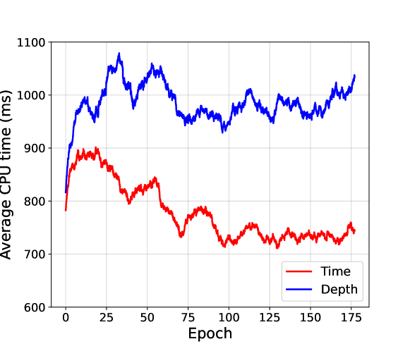
Figure 12: Average CPU time of proofs found by our model using different minimization objectives. When the model is trained to generate proofs that minimize the running time in Lean (red), the average proof time is significantly lower.

	Depth	Time
ring	21	20
norm_num	58	55
linarith	66	66
simp	62	38
refl	3	7
exact	4	17
apply	11	35
rewrite	20	65

Table 10: Qualitative comparison of the frequency of specific Lean tactics when using different minimization objective. Tactics in the upper half are slow automated tactics, while tactics in the bottom half are faster and simpler.

Appendix F Example Lean proofs

In this section, we show examples of proofs found by our model.

⬇

1theorem imo_1964_p1_2 (n : $\mathbb{N}$) : $\neg 7|2^{n}+1$ :=

2begin

3 rw nat.dvd_iff_mod_eq_zero,

4 rewrite [nat.add_mod, nat.mod_eq_of_lt],

5 obviously,

6 apply nat.strong_induction_on n,

7 induction n,

8 {

9 intros n IH,

10 cases n,

11 norm_num,

12 cases n,

13 norm_num,

14 rw [nat.succ_eq_add_one, pow_succ],

15 rw [nat.succ_eq_add_one, pow_succ],

16 induction n,

17 norm_num,

18 rw [nat.succ_eq_add_one, pow_succ],

19 norm_num [nat.mul_mod, ←mul_assoc],

20 contrapose! IH,

21 refine $\langle$n_n, nat.lt_succ_iff.mpr _, IH$\rangle$,

22 exact nat.le_succ_of_le (nat.le_succ _),

23 },

24 exact n_ih,

25end

Figure 13: A proof of the imo_1964_p1_2 problem found by our model. The model shows that for any value of $n\in\mathbb{N}$, $2^{n}+1$ is not divisible by $7$, by showing that $2^{n}\bmod 7+1\neq 0$, and $2^{n}\bmod 7+1<7$. The second part of the proof uses strong induction and the fact that $2^{n}\equiv 2^{n+3}\mod 7$. We provide a version of the proof that was automatically cleaned by removing unnecessary tactics and tactic arguments.

⬇

1theorem imo_2001_p6

2 (a b c d : ℕ)

3 (h₀ : 0 < a ∧ 0 < b ∧ 0 < c ∧ 0 < d)

4 (h₁ : d < c)

5 (h₂ : c < b)

6 (h₃ : b < a)

7 (h₄ : a * c + b * d = (b + d + a - c) * (b + d - a + c)) :

8 ¬ nat.prime (a * b + c * d) :=

9begin

10 contrapose h₄,

11 rw mul_comm,

12 simp [nat.prime, not_le_of_gt h₀.1, not_forall, not_le_of_gt h₃,

13 nat.mul_sub_right_distrib, nat.add_comm],

14 contrapose! h₄,

15 contrapose! h₄,

16 apply has_lt.lt.ne,

17 apply nat.lt_sub_right_of_add_lt,

18 nlinarith,

19end

Figure 14: A proof found by our model of another IMO problem in miniF2F. Although the proof is valid, the statement is erroneous. The hypothesis $h_{4}$ : $b+d-a+c$ actually represents $\max(b+d-a,0)+c$. This is due to Lean’s nat type behaviour where $(a:\mathbb{N})-(b:\mathbb{N})=(0:\mathbb{N})$ if $b\geq a$. This makes the exercise easier than it should be, and the proof is no longer valid on the fixed statement.

References

- Kempe [1879] Alfred B Kempe. On the geographical problem of the four colours. American journal of mathematics, 2(3):193–200, 1879.
- Voevodsky [2011] Vladimir Voevodsky. Univalent foundations of mathematics. In International Workshop on Logic, Language, Information, and Computation, pages 4–4. Springer, 2011.
- Hales et al. [2017] Thomas Hales, Mark Adams, Gertrud Bauer, Dat Dang, John Harrison, Truong Hoang, Cezary Kaliszyk, Victor Magron, Sean McLaughlin, Thang Nguyen, Truong Nguyen, Tobias Nipkow, Steven Obua, Joseph Pleso, Jason Rute, Alexey Solovyev, An Ta, Trân Trung, Diep Trieu, and Roland Zumkeller. A formal proof of the kepler conjecture. Forum of Mathematics, Pi, 5, 01 2017. doi: 10.1017/fmp.2017.1.
- Moura et al. [2015] Leonardo de Moura, Soonho Kong, Jeremy Avigad, Floris van Doorn, and Jakob von Raumer. The lean theorem prover (system description). In International Conference on Automated Deduction, pages 378–388. Springer, 2015.
- Knuth and Moore [1975] Donald E Knuth and Ronald W Moore. An analysis of alpha-beta pruning. Artificial intelligence, 6(4):293–326, 1975.
- Abramson and Korf [1987] Bruce Abramson and Richard E Korf. A model of two-player evaluation functions. In AAAI, pages 90–94, 1987.
- Silver et al. [2018] David Silver, Thomas Hubert, Julian Schrittwieser, Ioannis Antonoglou, Matthew Lai, Arthur Guez, Marc Lanctot, Laurent Sifre, Dharshan Kumaran, Thore Graepel, et al. A general reinforcement learning algorithm that masters chess, shogi, and go through self-play. Science, 362(6419):1140–1144, 2018.
- Zheng et al. [2021] Kunhao Zheng, Jesse Michael Han, and Stanislas Polu. Minif2f: a cross-system benchmark for formal olympiad-level mathematics. arXiv preprint arXiv:2109.00110, 2021.
- Gilmore [1960] P. C. Gilmore. A proof method for quantification theory: Its justification and realization. IBM J. Res. Dev., 4(1):28–35, jan 1960. ISSN 0018-8646. doi: 10.1147/rd.41.0028. URL https://doi.org/10.1147/rd.41.0028.
- Davis and Putnam [1960] Martin Davis and Hilary Putnam. A computing procedure for quantification theory. J. ACM, 7(3):201–215, jul 1960. ISSN 0004-5411. doi: 10.1145/321033.321034. URL https://doi.org/10.1145/321033.321034.
- Schulz [2002] Stephan Schulz. E—a brainiac theorem prover. AI Commun., 15(2–3):111–126, 2002.
- Riazanov and Voronkov [2001] Alexandre Riazanov and Andrei Voronkov. Vampire 1.1 (system description). In IJCAR, 2001.
- Nipkow et al. [2002] Tobias Nipkow, Lawrence C. Paulson, and Markus Wenzel. Isabelle/HOL: A Proof Assistant for Higher-Order Logic, volume 2283 of LNCS. Springer, 2002.
- Bertot and Castéran [2013] Yves Bertot and Pierre Castéran. Interactive theorem proving and program development: Coq’Art: the calculus of inductive constructions. Springer Science & Business Media, 2013.
- Radford et al. [2019] Alec Radford, Jeffrey Wu, Rewon Child, David Luan, Dario Amodei, Ilya Sutskever, et al. Language models are unsupervised multitask learners. OpenAI blog, 1(8):9, 2019.
- Polu and Sutskever [2020] Stanislas Polu and Ilya Sutskever. Generative language modeling for automated theorem proving. arXiv preprint arXiv:2009.03393, 2020.
- Han et al. [2021] Jesse Michael Han, Jason Rute, Yuhuai Wu, Edward W Ayers, and Stanislas Polu. Proof artifact co-training for theorem proving with language models. arXiv preprint arXiv:2102.06203, 2021.
- Polu et al. [2022] Stanislas Polu, Jesse Michael Han, Kunhao Zheng, Mantas Baksys, Igor Babuschkin, and Ilya Sutskever. Formal mathematics statement curriculum learning. arXiv preprint arXiv:2202.01344, 2022.
- Whalen [2016] Daniel Whalen. Holophrasm: a neural automated theorem prover for higher-order logic. arXiv preprint arXiv:1608.02644, 2016.
- Bansal et al. [2019] Kshitij Bansal, Sarah Loos, Markus Rabe, Christian Szegedy, and Stewart Wilcox. Holist: An environment for machine learning of higher order logic theorem proving. In International Conference on Machine Learning, pages 454–463. PMLR, 2019.
- Harrison [1996] John Harrison. Hol light: A tutorial introduction. In International Conference on Formal Methods in Computer-Aided Design, pages 265–269. Springer, 1996.
- Gauthier et al. [2021] Thibault Gauthier, Cezary Kaliszyk, Josef Urban, Ramana Kumar, and Michael Norrish. Tactictoe: learning to prove with tactics. Journal of Automated Reasoning, 65(2):257–286, 2021.
- Chvalovskỳ et al. [2021] Karel Chvalovskỳ, Jan Jakubův, Miroslav Olšák, and Josef Urban. Learning theorem proving components. In International Conference on Automated Reasoning with Analytic Tableaux and Related Methods, pages 266–278. Springer, 2021.
- Sutskever et al. [2014] Ilya Sutskever, Oriol Vinyals, and Quoc V Le. Sequence to sequence learning with neural networks. Advances in neural information processing systems, 27, 2014.
- Lachaux et al. [2020] Marie-Anne Lachaux, Baptiste Roziere, Lowik Chanussot, and Guillaume Lample. Unsupervised translation of programming languages. arXiv preprint arXiv:2006.03511, 2020.
- Saxton et al. [2019] David Saxton, Edward Grefenstette, Felix Hill, and Pushmeet Kohli. Analysing mathematical reasoning abilities of neural models. In International Conference on Learning Representations, 2019. URL https://openreview.net/forum?id=H1gR5iR5FX.
- Lample and Charton [2020] Guillaume Lample and François Charton. Deep learning for symbolic mathematics. In International Conference on Learning Representations, 2020. URL https://openreview.net/forum?id=S1eZYeHFDS.
- d’Ascoli et al. [2022] Stéphane d’Ascoli, Pierre-Alexandre Kamienny, Guillaume Lample, and François Charton. Deep symbolic regression for recurrent sequences. arXiv preprint arXiv:2201.04600, 2022.
- Petersen et al. [2021] Brenden K Petersen, Mikel Landajuela Larma, Terrell N. Mundhenk, Claudio Prata Santiago, Soo Kyung Kim, and Joanne Taery Kim. Deep symbolic regression: Recovering mathematical expressions from data via risk-seeking policy gradients. In International Conference on Learning Representations, 2021. URL https://openreview.net/forum?id=m5Qsh0kBQG.
- Charton et al. [2020] François Charton, Amaury Hayat, and Guillaume Lample. Learning advanced mathematical computations from examples. arXiv preprint arXiv:2006.06462, 2020.
- Megill and Wheeler [2019] Norman D. Megill and David A. Wheeler. Metamath: A Computer Language for Mathematical Proofs. Lulu Press, Morrisville, North Carolina, 2019. http://us.metamath.org/downloads/metamath.pdf.
- mathlib Community [2020] The mathlib Community. The lean mathematical library. In Proceedings of the 9th ACM SIGPLAN International Conference on Certified Programs and Proofs. ACM, jan 2020. doi: 10.1145/3372885.3373824. URL https://doi.org/10.1145%2F3372885.3373824.
- Silver et al. [2017] David Silver, Thomas Hubert, Julian Schrittwieser, Ioannis Antonoglou, Matthew Lai, Arthur Guez, Marc Lanctot, Laurent Sifre, Dharshan Kumaran, Thore Graepel, et al. Mastering chess and shogi by self-play with a general reinforcement learning algorithm. arXiv preprint arXiv:1712.01815, 2017.
- Grill et al. [2020] Jean-Bastien Grill, Florent Altché, Yunhao Tang, Thomas Hubert, Michal Valko, Ioannis Antonoglou, and Rémi Munos. Monte-carlo tree search as regularized policy optimization. In International Conference on Machine Learning, pages 3769–3778. PMLR, 2020.
- Chaslot et al. [2008] Guillaume MJ-B Chaslot, Mark HM Winands, and HJVD Herik. Parallel monte-carlo tree search. In International Conference on Computers and Games, pages 60–71. Springer, 2008.
- Vaswani et al. [2017] Ashish Vaswani, Noam Shazeer, Niki Parmar, Jakob Uszkoreit, Llion Jones, Aidan N Gomez, Łukasz Kaiser, and Illia Polosukhin. Attention is all you need. In Advances in neural information processing systems, pages 5998–6008, 2017.
- Nair et al. [2015] Arun Nair, Praveen Srinivasan, Sam Blackwell, Cagdas Alcicek, Rory Fearon, Alessandro De Maria, Vedavyas Panneershelvam, Mustafa Suleyman, Charles Beattie, Stig Petersen, et al. Massively parallel methods for deep reinforcement learning. arXiv preprint arXiv:1507.04296, 2015.
- Sennrich et al. [2015] Rico Sennrich, Barry Haddow, and Alexandra Birch. Neural machine translation of rare words with subword units. In Proceedings of the 54th Annual Meeting of the Association for Computational Linguistics, pages 1715–1725, 2015.
- Devlin et al. [2018] Jacob Devlin, Ming-Wei Chang, Kenton Lee, and Kristina Toutanova. Bert: Pre-training of deep bidirectional transformers for language understanding. CoRR, abs/1810.04805, 2018.
- Lample and Conneau [2019] Guillaume Lample and Alexis Conneau. Cross-lingual language model pretraining. arXiv preprint arXiv:1901.07291, 2019.
- Song et al. [2019] Kaitao Song, Xu Tan, Tao Qin, Jianfeng Lu, and Tie-Yan Liu. Mass: Masked sequence to sequence pre-training for language generation. arXiv preprint arXiv:1905.02450, 2019.
- Kasai et al. [2020] Jungo Kasai, Nikolaos Pappas, Hao Peng, James Cross, and Noah A Smith. Deep encoder, shallow decoder: Reevaluating non-autoregressive machine translation. arXiv preprint arXiv:2006.10369, 2020.
- Kingma and Ba [2014] Diederik Kingma and Jimmy Ba. Adam: A method for stochastic optimization. arXiv preprint arXiv:1412.6980, 2014.
- Srivastava et al. [2014] Nitish Srivastava, Geoffrey Hinton, Alex Krizhevsky, Ilya Sutskever, and Ruslan Salakhutdinov. Dropout: a simple way to prevent neural networks from overfitting. The journal of machine learning research, 15(1):1929–1958, 2014.
- Fan et al. [2020] Angela Fan, Edouard Grave, and Armand Joulin. Reducing transformer depth on demand with structured dropout. In International Conference on Learning Representations, 2020. URL https://openreview.net/forum?id=SylO2yStDr.
- Paszke et al. [2017] Adam Paszke, Sam Gross, Soumith Chintala, Gregory Chanan, Edward Yang, Zachary DeVito, Zeming Lin, Alban Desmaison, Luca Antiga, and Adam Lerer. Automatic differentiation in pytorch. NIPS 2017 Autodiff Workshop, 2017.
- Wang and Gelly [2007] Yizao Wang and Sylvain Gelly. Modifications of uct and sequence-like simulations for monte-carlo go. In 2007 IEEE Symposium on Computational Intelligence and Games, pages 175–182. IEEE, 2007.
- Winands et al. [2008] Mark HM Winands, Yngvi Björnsson, and Jahn-Takeshi Saito. Monte-carlo tree search solver. In International Conference on Computers and Games, pages 25–36. Springer, 2008.