Logical Reasoning with Span-Level Predictions for
Interpretable and Robust NLI Models

Abstract

Current Natural Language Inference (NLI) models achieve impressive results, sometimes outperforming humans when evaluating on in-distribution test sets. However, as these models are known to learn from annotation artefacts and dataset biases, it is unclear to what extent the models are learning the task of NLI instead of learning from shallow heuristics in their training data. We address this issue by introducing a logical reasoning framework for NLI, creating highly transparent model decisions that are based on logical rules. Unlike prior work, we show that improved interpretability can be achieved without decreasing the predictive accuracy. We almost fully retain performance on SNLI, while also identifying the exact hypothesis spans that are responsible for each model prediction. Using the e-SNLI human explanations, we verify that our model makes sensible decisions at a span level, despite not using any span labels during training. We can further improve model performance and span-level decisions by using the e-SNLI explanations during training. Finally, our model is more robust in a reduced data setting. When training with only 1,000 examples, out-of-distribution performance improves on the MNLI matched and mismatched validation sets by 13% and 16% relative to the baseline. Training with fewer observations yields further improvements, both in-distribution and out-of-distribution.

1 Introduction

The task of Natural Language Inference (NLI) involves reasoning across a premise and hypothesis, determining the relationship between the two sentences. Either the hypothesis is implied by the premise (entailment), the hypothesis contradicts the premise (contradiction), or the hypothesis is neutral to the premise (neutral). NLI can be a highly challenging task, requiring lexical, syntactic and logical reasoning, in addition to sometimes requiring real-world knowledge Dagan et al. (2005). While neural NLI models perform well on in-distribution test sets, this does not necessarily mean they have a strong understanding of the underlying task. Instead, NLI models are known to learn from annotation artefacts (or biases) in their training data Gururangan et al. (2018); Poliak et al. (2018). Models can therefore be right for the wrong reasons McCoy et al. (2019), with no guarantees about the reasons for each prediction, or whether the predictions are based on a genuine understanding of the task. We address this issue with our logical reasoning framework, creating more interpretable NLI models that definitively show the specific logical atoms responsible for each model prediction.

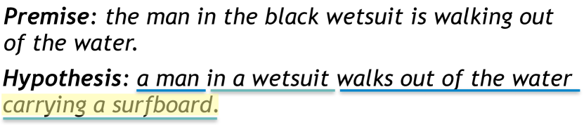
Figure 1: Example of a hypothesis segmented into spans, with the four different hypothesis spans underlined. The model predicts the neutral class only for ‘carrying a surfboard.’, as this is not implied by the premise.

One challenge when applying a logical approach to NLI is determining the choice of logical atoms. When constructing examples from knowledge bases, the relationships between entities in the knowledge base can be used as logical atoms Rocktäschel and Riedel (2017); in synthetic fact-based datasets, each fact can become a logical atom Clark et al. (2020); Talmor et al. (2020). Neither approach would be suitable for SNLI Bowman et al. (2015), which requires reasoning over gaps in explicitly stated knowledge Clark et al. (2020), with observations covering a range of topics and using different forms of reasoning. Instead, our novel logical reasoning framework considers spans of the hypothesis as logical atoms. We determine the class of each premise-hypothesis pair based entirely on span-level decisions, identifying exactly which parts of a hypothesis are responsible for each model decision. By providing a level of assurance about the cause of each prediction, we can better understand the reasons for the correct predictions and highlight any mistakes or misconceptions being made. Using the e-SNLI dataset Camburu et al. (2018), we assess the performance of our span-level predictions, ensuring that the decisions about each hypothesis span align with human explanations.

To summarise our findings: 1) Our Span Logical Reasoning framework (SLR-NLI) produces highly interpretable models, identifying exactly which parts of the hypothesis are responsible for each model prediction. 2) SLR-NLI almost fully retains performance on SNLI, while also performing well on the SICK dataset Marelli et al. (2014). This contrasts with previous work, where the inclusion of logical frameworks result in substantially worse performance. 3) Evaluating the SLR-NLI predictions at a span level shows that the span-level decisions are consistent with human explanations, with further improvements if e-SNLI explanations are used during training. 4) SLR-NLI improves model robustness when training in a reduced data setting, improving performance on unseen, out-of-distribution NLI datasets.

2 Span Logical Reasoning

Inspired by previous work on error detection Rei and Søgaard (2018, 2019); Pislar and Rei (2020); Bujel et al. (2021), we construct models for detecting spans of the hypothesis that either contradict the premise (contradiction spans) or are not implied by the premise (neutral spans). We train the model with sentence-level labels while also using auxiliary losses that guide the model behaviour at the span level. As no span labels are provided in the SNLI training data, we supervise our SLR-NLI model at a span level using logical rules, for example requiring a contradiction example to include at least one contradiction span. The model is evaluated based on the span-level decisions for each logical atom.

2.1 Span-level Approach

We consider each hypothesis as a set of spans ${s_{1},s_{2},s_{3},...,s_{m}}$ where each span is a consecutive sequence of words in the hypothesis. For example, in Figure 1 the hypothesis ‘a man in a wetsuit walks out of the water carrying a surfboard.’ contains the following spans: ‘a man’, ‘in a wetsuit’, ‘walks out of the water’, ‘carrying a surfboard.’. Each span $s_{i}$ has a label of either entailment, contradiction or the neutral class. In practice, there are no predefined spans in NLI datasets, nor are there labels for any chosen spans. As a result, we propose a method of dividing hypotheses into spans, introducing a semi-supervised method to identify entailment relationships at this span level. In the example provided in Figure 1, $s_{4}$=‘carrying a surfboard.’ has a neutral label, while the other spans have an entailment label.

We observe that a hypothesis has a contradiction label if any span present in that hypothesis has a label of contradiction. Similarly, if a hypothesis contains a span with a neutral label and no span with a contradiction label, then the hypothesis belongs to the neutral class. Therefore, a hypothesis only has an entailment class if there are no spans present with span labels of either contradiction or neutral.

When evaluating a hypothesis-premise pair in the test data, our model makes discrete entailment decisions about each span in the hypothesis. The sentence-level label is then assigned based on the presence of any neutral or contradiction spans. This method highlights the exact parts of a hypothesis responsible for each entailment decision.

2.2 Span Selection

We identify spans based on the presence of noun phrases in the hypothesis. Initially, the hypothesis is segmented into spans, with a span provided for each noun phrase which includes both the noun phrase and any preceding text since the last noun phrase. The first span includes any text up to and including the first noun phrase, while the last span includes any text after the last noun phrase. Noun phrases are identified using spaCy.

However, the most appropriate segmentation of a hypothesis may depend on the corresponding premise, and in some cases, we may need to consider long-range dependencies across the sentence. As a result, we also provide additional spans that are constructed from combinations of consecutive spans. For the example in Figure 1, this means also including spans such as ‘a man in a wetsuit’ and ‘walks out of the water carrying a surfboard.’. We set the number of consecutive spans that are included as a hyper-parameter. We also experiment with a dropout mechanism that randomly masks these additional, consecutive spans for a proportion of the training examples (10%). This ensures that the model still makes sensible decisions at the most granular span level, while also being able to learn from long-range dependencies across the sentences.

2.3 Modelling Approach

A BERT model Devlin et al. (2019) is used for encoding the NLI premise together with each specific hypothesis span, masking the parts of the hypothesis that are not included in the given span. The BERT model provides a [CLS] representation $h_{i}$ for each span $i$. A linear layer is applied to these representations to provide logits $L_{n,i}$ and $L_{c,i}$ for each span, representing the neutral and contradiction classes respectively.

A separate attention layer is created for both the neutral and contradiction classes that attend to each span-level output. The neutral attention layer attends more to neutral spans, while the contradiction attention layer attends more to contradiction spans. Both the neutral and contradiction attention layers consider the same [CLS] representation $h_{i}$.

The two attention layers use the same architecture, with details provided below for the neutral (n) attention layer. Our span-level predictions will be based on the unnormalized attention weights $\widetilde{a}_{n,i}$, which are calculated as:

$$\widetilde{a}_{n,i}=\sigma{(W_{n,2}(\tanh{(W_{n,1}h_{i}+b_{n,1})})+b_{n,2})}$$ (1)

where $W_{n,1}$, $W_{n,2}$, $b_{n,1}$, and $b_{n,2}$ are trainable parameters. Equation 1 uses a sigmoid so that the output is in the range between 0 and 1 for binary classification. Upon normalisation, the attention weights ${a}_{n,i}$ define an attention distribution:

$$a_{n,i}=\frac{\widetilde{a}_{n,i}}{\sum_{k=1}^{m}\widetilde{a}_{n,k}}$$ (2)

These weights are used to create a logit, $L_{n}$:

$$L_{n}=\sum_{i=1}^{m}a_{n,i}L_{n,i}$$ (3)

Using a binary label $y_{n}$, indicating if the example is neutral or not, we create a sentence-level loss to optimise using the sentence labels:

$$\mathcal{L}_{n}^{\text{Sent}}=(\sigma(W_{n,3}\times L_{n}+b_{n,3})-y_{n})^{2}$$ (4)

We combine this with an auxiliary span loss on the model attention weights, $\mathcal{L}_{n}^{\text{Span}}$:

$$\mathcal{L}_{n}^{\text{Span}}=(\max_{i}(\widetilde{a}_{n,i})-y_{n})^{2}$$ (5)

The auxiliary span attention loss has the effect of encouraging the span-level unnormalized attention weights to be closer to zero for entailment examples. This supports our logical framework, which states that all entailment examples must only consist of entailment spans (i.e. with no contradiction or neutral spans). As neutral predictions require at least one neutral span, by supervising the maximum unnormalized attention weight we encourage one of the spans to be predicted as neutral if the sentence label is also neutral. The contradiction-detection attention layer behaves in a similar way, detecting the presence of contradiction spans.

We then combine together the auxiliary span attention loss with the sentence-level loss:

$$\mathcal{L}_{n}^{\text{Total}}=\mathcal{L}_{n}^{\text{Sent}}+\mathcal{L}_{n}^{\text{Span}}.$$ (6)

While our model evaluation exclusively makes predictions from the unnormalized attention weights for each span, we find in practice that including a sentence-level objective improves the span-level decisions. In particular, the sentence supervision influences the attention values directly in Equation 3, in addition to supervising the representations $h_{i}$. The sentence-level supervision does not have access to the full hypothesis, separately considering each span representation $h_{i}$. See Figure 2 for a model architecture diagram.

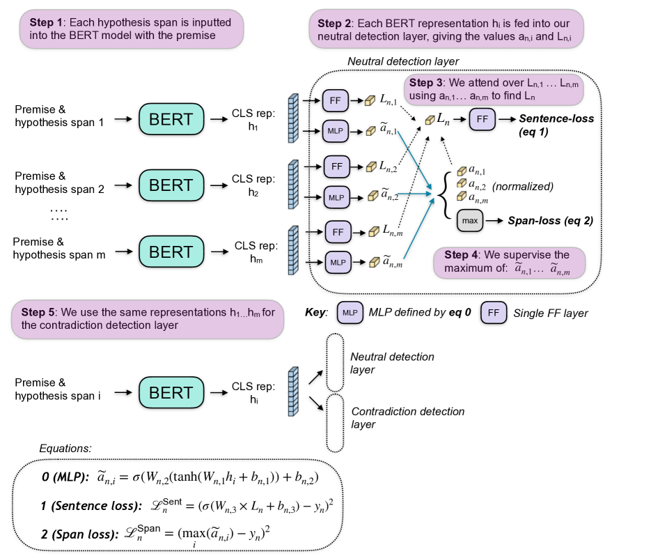
Figure 2: Model diagram describing the training process for SLR-NLI

2.4 Span-level Supervision with Human Explanations

To provide our model with more information about individual spans, we can use the e-SNLI Camburu et al. (2018) human explanations, with rationales highlighting the most important words in each hypothesis. Training models with the e-SNLI explanations can improve both model performance and robustness Stacey et al. (2022); Zhao and Vydiswaran (2021), although not all prior work has found these improvements Kumar and Talukdar (2020); Camburu et al. (2018); Carton et al. (2022). We assess whether the human explanations can help our model make better decisions at the span level, and also whether the explanations further improve the performance of SLR-NLI.

To incorporate the human explanations during training, we consider the highlighted word rationales for each hypothesis. If any of our SLR-NLI hypothesis spans contain all of the e-SNLI rationale, we assign the overall sentence label as the individual span label. If the hypothesis rationale is not a single consecutive span then we do not provide any supervision with the explanation, as we observe that only single-span rationales consistently align with the desired span-level labels.

Let $p_{i}$ be the value of 1 where the hypothesis rationale is fully contained within the $i$-th span, and 0 otherwise. Our neutral auxiliary e-SNLI loss $\mathcal{L}_{n}^{\text{e-SNLI}}$ is defined as:

$$\mathcal{L}_{n}^{\text{e-SNLI}}=\lambda^{\text{e-SNLI}}\sum_{i}{p_{i}(\widetilde{a}_{n,i}-y_{n})^{2}},$$

while $\mathcal{L}_{c}^{\text{e-SNLI}}$ is defined in a similar way, using $\widetilde{a}_{c,i}$ and $y_{c}$.

2.5 Training Process

Our neutral and contradiction attention models have two class labels, with $y_{n}$ and $y_{c}$ taking values of 0 or 1. ${y}_{n}=0$ when there are no neutral spans present, while ${y}_{n}=1$ when there is at least one neutral span. ${y}_{c}$ follows the same approach for the contradiction detection label.

For neutral NLI examples, we train our neutral-detection model using a sentence-level label of $y_{n}=1$. Using our logical framework, we also know that a neutral example cannot contain a contradiction span, as any example with a contradiction span would have a contradiction label. Therefore, we train our contradiction-detection model using a sentence-level label of $y_{c}=0$ for these examples. For contradiction examples, we do not train our neutral-detection attention model, as there may or may not be neutral spans present in addition to the contradiction spans. For entailment examples, we train both neutral and contradiction detection models using the labels $y_{n}=0$ and $y_{c}=0$.

Therefore, for neutral or entailment examples we consider the total of both $\mathcal{L}_{n}^{\text{Total}}$ and $\mathcal{L}_{c}^{\text{Total}}$, whereas for the contradiction class we only consider $\mathcal{L}_{c}^{\text{Total}}$.

2.6 Evaluation

We evaluate each NLI sentence based exclusively on our span-level decisions. Specifically, an NLI hypothesis is classified as the contradiction class if any of the unnormalized attention weights are predicted as contradiction ($\widetilde{a}_{c,i}>0.5$). If there are no contradiction spans present, an NLI example is classified as neutral if there exists at least one neutral span ($\widetilde{a}_{n,i}>0.5)$. Otherwise, the NLI example is classified as entailment.

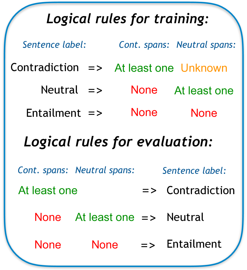
Figure 3: Our logical rules for training and evaluation. The logical rules for training: 1) for contradiction sentences we use a label of $y_{c}$ = 1, but do not supervise with a value of $y_{n}$, 2) for neutral sentences, we supervise with $y_{c}$ = 0 and $y_{n}$ = 1, and 3) for entailment sentences we supervise with $y_{c}$ = 0 and $y_{n}$ = 0. The logical rules for evaluation: 1) the presence of any contradiction span implies the sentence prediction is contradiction, 2) if no contradiction span is present, the presence of a neutral span implies a neutral sentence prediction, and 3) otherwise we have an entailment prediction.

The sentence-level logits $L_{n}$ or $L_{c}$ are only used during training and discarded for evaluation – they consider information across all the spans and therefore do not allow for a deterministic evaluation of which spans are responsible for the model predictions. The logical rules used in both training and evaluation follow from the inherent nature of NLI (these rules are summarised in Figure 3).

3 Related Work

3.1 NLI with Neural Theorem Provers

Neural theorem provers can effectively solve a range of natural language tasks Rocktäschel and Riedel (2017); Weber et al. (2019); Minervini et al. (2020b, a), many of which could be recast in a similar form to NLI. These datasets are often built from knowledge graphs Sinha et al. (2019); Bouchard et al. (2015); Kok and Domingos (2007), for example identifying relationships between characters in short stories Sinha et al. (2019). Non-neural theorem provers have also shown promising results on the SICK dataset (Martínez-Gómez et al., 2017; Abzianidze, 2020, 2017; Yanaka et al., 2018), although these methods cannot be easily translated to SNLI, which covers a wide range of topics and uses various forms of reasoning.

3.2 Monotonic Reasoning with NLI

Using monotonic reasoning involves matching components of the hypothesis and premise, and using external knowledge from resources including WordNet Miller (1995) to determine the entailment relationships between corresponding parts of both sentences Kalouli et al. (2020); Hu et al. (2020); Chen et al. (2021). To improve performance, this logical approach can be combined with traditional neural models, learning which examples would benefit from a neural approach rather than using logical rules Kalouli et al. (2020), or using neural models to decide the class of examples where entailment and contradiction classes have not been detected Hu et al. (2020). A hybrid approach can improve performance, but at the expense of the interpretability benefits. Logic models using monotonic reasoning are mostly evaluated on SICK and other datasets with a small number of differences between the premise and hypothesis. While our logical framework is not specifically designed for these datasets, we show our performance on SICK still remains competitive with this prior work.

3.3 Logical Reasoning with SNLI

Previous work has applied logical reasoning techniques to SNLI, but with performance substantially below baseline levels. Feng et al. (2022) segment a hypothesis into spans, choosing one of seven logical relations for each hypothesis span. A logical relation is predicted for each span using a GPT-2 model Radford et al. (2019) which considers the premise, the given span and all prior hypothesis spans, with reinforcement learning training this span-level behaviour (Feng et al., 2022). Previous work also predicts the seven logical relations for individual words rather than for hypothesis spans Feng et al. (2020).

Closest to our work, Wu et al. (2021) label spans as entailment, neutral or contradiction, evaluating at a sentence level based on the presence of neutral or contradiction spans. Our substantial performance improvements compared to Wu et al. (2021) reflect our different approaches to supervising at a span level. Wu et al. (2021) provide each span model with information about the entire premise and hypothesis, in addition to a hypothesis span and a corresponding premise span. The span label is then predicted using a three-class classifier. In comparison, we create separate additional attention layers for neutral and contradiction span detection, combining together multiple different losses to supervise at both the sentence and span level. As we consider neutral and contradiction span detection as separate binary tasks, we also introduce logical rules during training which include not supervising our neutral detection model for contradiction examples, and how a neutral label means there are no contradiction spans present.

We directly compare our results to Feng et al. (2020), Wu et al. (2021) and Feng et al. (2022).

4 Experiments

We train the SLR-NLI model either using SNLI Bowman et al. (2015) or SICK Marelli et al. (2014). SNLI is a large corpus of 570k observations, with a diverse range of reasoning strategies required to understand the relationship between the premise and hypothesis. Image captions are used for premises, with annotators asked to create a hypothesis for each class for each given premise. In contrast, SICK has 10k observations and initially uses sentence pairs from image captions and video descriptions, with additional sentence pairs generated by applying a series of rules, including replacing nouns with pronouns and simplifying verb phrases. As a result, entailment and contradiction examples in SICK are often the same except with one or two small changes. Previous work exploits this similarity, using logical reasoning to identify the contradiction and entailment examples Chen et al. (2021); Hu et al. (2020). Compared to this setting, SNLI provides a more challenging dataset for applying logical reasoning.

We further experiment with training our model in a reduced data setting, motivated by the hypothesis that forcing our model to learn at a span-level will make better use of a smaller number of examples. We expect SLR-NLI to be more robust in a reduced data setting, with existing models known to rely on dataset biases when overfitting to small datasets Utama et al. (2020b). For the reduced data experiments, we train SLR-NLI with 100 and 1,000 examples from SICK or SNLI, evaluating out-of-distribution performance on other unseen NLI datasets including SNLI-hard Gururangan et al. (2018), MNLI Williams et al. (2018) and HANS McCoy et al. (2019). As no explanations are provided for SICK, we only use explanations when training on SNLI (reported as SLR-NLI-eSNLI).

For SICK, when we consider out-of-distribution performance we evaluate on the corrected SICK dataset Hu et al. (2020), with labels manually corrected by Hu et al. (2020) and Kalouli et al. (2017). However, for a fair comparison to previous work, we use the original SICK dataset when evaluating in-distribution performance from SICK.

To validate that the model is making sensible decisions at a span level, we compare the span-level predictions to the e-SNLI human explanations. For each single-span hypothesis rationale in e-SNLI, we consider each model span containing this entire rationale. Each span that does contain the rationale is evaluated, with its span predictions compared to the sentence-level label.

In summary, we consider the following research questions: 1) Does our interpretable SLR-NLI model retain performance on SNLI? 2) Is SLR-NLI a flexible approach that can also work on SICK? 3) Does SLR-NLI improve performance in a reduced data setting? 4) In the reduced data setting, does SLR-NLI also improve robustness? 5) Does SLR-NLI make sensible decisions at a span level?

5 Results

Accuracy	SNLI	$\Delta$
BERT (baseline)	90.77
Feng et al. (2020)	81.2	-9.57
Wu et al. (2021)	84.53	-6.24
Feng et al. (2022)	87.8	-2.97
SLR-NLI	90.33	-0.44
SLR-NLI+esnli	90.49	-0.28

Table 1: Performance (accuracy) on the SNLI test-set from SLR-NLI, with and without the additional e-SNLI supervision during training. Each condition is tested across 5 random seeds, including the baseline.

Accuracy	SICK	$\Delta$
BERT (baseline)	85.52
Hybrid systems
Hu et al. (2020)+BERT	85.4	-0.1
Kalouli et al. (2020)	86.5	+1.0
Logic-based systems
Hu et al. (2020)	77.2	-8.3
Abzianidze (2017)	81.4	-4.1
Martínez-Gómez et al. (2017)	83.1	-2.4
Yanaka et al. (2018)	84.3	-1.2
Abzianidze (2020)	84.4	-1.1
Chen et al. (2021)	90.3	+4.8
SLR-NLI	85.43	-0.09

Table 2: Performance (accuracy) of SLR-NLI on the SICK dataset compared to previous work. Results for SLR-NLI-eSNLI are not provided, as the e-SNLI explanations are specific to SNLI. Results are an average from across 5 random seeds.

Dataset	Baseline	SLR-NLI
SICK	81.11	81.33
SNLI-dev	38.50	46.96$\ddagger$
SNLI-test	38.17	46.88$\ddagger$
SNLI-hard	38.34	44.58$\ddagger$
MNLI-mismatch.	40.90	47.85$\dagger$
MNLI-match.	39.72	46.51$\dagger$
HANS	53.22	50.61

Table 3: Accuracy of SLR-NLI compared to a BERT baseline when training with 1,000 SICK examples. The best results are in bold. All results are an average across 5 random seeds. Statistically significant results with $p<0.05$ are denoted with $\dagger$, while results with $p<0.01$ are denoted with $\ddagger$, using a two-tailed bootstrapping hypothesis test Efron and Tibshirani (1993).

Model	In-Distribution		Out-of-Distribution
	SNLI-dev	SNLI-test	SNLI-hard	MNLI-mis.	MNLI-mat.	SICK	HANS
Baseline	73.98	73.90	59.25	49.17	48.46	52.19	50.27
PoE	60.79	61.26	54.44	41.74	42.03	45.92	50.26
Reweight.	70.69	70.86	59.83	46.99	47.12	48.65	50.03
Conf Reg.	57.32	57.51	49.61	38.05	38.54	38.93	50.84
SLR-NLI-eSNLI	74.22	74.05	59.51	57.05$\dagger$	54.76$\dagger$	52.23	50.00

Table 4: Accuracy of SLR-NLI-eSNLI compared to a BERT baseline when training with 1,000 SNLI examples. The best results for each dataset are in bold. We compare to a Product of Experts (Clark et al., 2019), Example Reweighting Clark et al. (2019) and Confidence Regularization Utama et al. (2020a). All results are an average across 5 random seeds. For SLR-NLI-eSNLI compared to the baseline, statistically significant results with $p<0.05$ are denoted with $\dagger$, while results with $p<0.01$ are denoted with $\ddagger$, using a two-tailed bootstrapping hypothesis test Efron and Tibshirani (1993).

Model	Sent. acc.	Span acc.	F-macro	F-ent	F-neut	F-cont
SLR-NLI (Zero-shot)	90.33	84.75	84.61	81.74	84.80	87.27
SLR-NLI + dropout (Zero-shot)	90.33	87.91	87.81	85.96	86.52	90.94
SLR-NLI-eSNLI (Supervised)	90.49	88.29	88.17	86.24	86.99	91.28

Table 5: Span-level performance of SLR-NLI-eSNLI compared to SLR-NLI. Span performance is evaluated on the three e-SNLI explanations available for each test observation after training on SNLI. A version of SLR-NLI with a dropout mechanism applied is also included. All results are an average across 5 random seeds.

5.1 Performance on SNLI and SICK

SLR-NLI achieves in-distribution results very close to the standard BERT model on the SNLI test set, with 90.33% accuracy compared to the baseline of 90.77% (Table 1). This result outperforms prior work on logical reasoning for SNLI, as the inclusion of logical frameworks has previously resulted in large drops in performance Feng et al. (2022); Wu et al. (2021); Feng et al. (2020). We achieve this level of performance without training or evaluating on the full premise and hypothesis pairs. When training with the e-SNLI explanations, we see an additional improvement in accuracy (90.49%).

SLR-NLI compares favourably to prior logical reasoning work on SICK, despite these baselines being specifically designed for this dataset (Table 2). For example, Chen et al. (2021) aims to bridge the differences between a hypothesis and premise, an approach not possible with SNLI. The strong performance of SLR-NLI on both SNLI and SICK shows the flexibility of this approach across different NLI datasets. As SLR-NLI is a model agnostic framework, we also combine SLR-NLI-eSNLI with a better performing DEBERTa model He et al. (2021). The DeBERTa-base model accuracy is 91.65%, compared to 91.48% for SLR-NLI-eSNLI (-0.17%). This difference in performance is smaller than for BERT (-0.28%).

5.2 Reduced Data Setting

In a reduced data setting, training SLR-NLI-eSNLI with 1,000 SNLI observations, there are significant out-of-distribution improvements on MNLI matched and mismatched with no loss of performance in-distribution (see Table 4). We show that this improved robustness contrasts with common debiasing methods, including Product of Experts Clark et al. (2019); Mahabadi et al. (2020), Example Reweighting Clark et al. (2019), and Confidence Regularization Utama et al. (2020a), each trained with a hypothesis-only shallow classifier. When training on SICK, we see out-of-distribution improvements on MNLI-matched, MNLI-mismatched, SNLI-dev, SNLI-test and SNLI-hard (see Table 3). As there is no clear hypothesis-only bias for SICK Belinkov et al. (2019), we do not perform the same comparison to previous robustness work. In-distribution improvements are also observed when training with only 100 SNLI observations, where performance is 18% higher relative to the baseline, with similar results observed when training on SICK. Out-of-distribution improvements also increase when training with fewer observations (complete results are available in the Appendix).

The only dataset where SLR-NLI performed worse than the baseline was HANS, where each hypothesis consists of words that are also in the premise. For example, the premise of ‘the doctor was paid by the actor’ is accompanied by the hypothesis ‘the doctor paid the actor’ McCoy et al. (2019). In these examples, evaluating on the smaller spans provides no additional benefit.

6 Analysis

6.1 Span-Level Evaluation

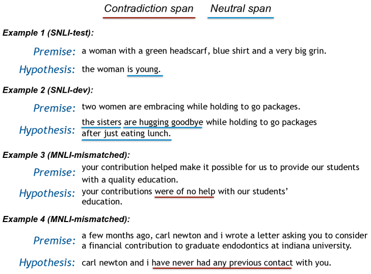
Figure 4: Span and sentence level predictions for SNLI-test, SNLI-dev and MNLI-mismatched (out-of-distribution). Each of the four examples above are correctly predicted by SLR-NLI-eSNLI.

Even without additional supervision from e-SNLI, SLR-NLI performs well at a span level, with 84.75% accuracy in a zero-shot setting (Table 5). This shows that human explanations are not required for the model to make sensible decisions at a span level. With the additional e-SNLI supervision, SLR-NLI-eSNLI reaches a span-level accuracy of 88.29%. We observe that without the additional e-SNLI supervision, the model tends to rely more on the longer spans that consist of consecutive smaller spans. To mitigate this issue, we experiment with a dropout mechanism during training which randomly masks large spans consisting of consecutive smaller spans, encouraging the model to also make sensible decisions at the most granular span level. In 10% of observations, all such large spans are masked, leaving only smaller spans as the model input. This dropout mechanism improves span performance to 87.91%, although the sentence-level performance does not improve in tandem (Table 5).

6.2 Model Interpretability

The main advantage of our span-level approach is the interpretability of the model predictions, allowing us to understand which specific parts of the hypothesis are responsible for each predicted label. We define explanation spans as the set of the smallest neutral and contradiction spans such that any longer span that is predicted as neutral or contradiction contains one of these spans. As a result, we only choose longer, multi-segment spans when there are no smaller spans that explain the model decisions. For contradiction predictions, we only include contradiction spans in our explanations.

As shown in Figure 4, Example 1, SLR-NLI-eSNLI consistently makes sensible span-level predictions for easier, shorter hypotheses. We therefore show the results of a longer example (Example 2), along with two out-of-distribution examples from the MNLI-mismatched set (Examples 3 and 4). In each case, the model is making correct decisions in line with our human expectations. To provide an unbiased sample of the span-level explanations, we show the first eight neutral and contradiction examples from SNLI-test in the Appendix.

A qualitative analysis shows that some incorrect predictions are a result of subjective labels in the dataset, for example, the model does not find that people walking behind a car implies that the people are necessarily on a street, whereas this example is entailed in SNLI. We also find that the model does not always perform well when evaluating the gender of the people mentioned in the premise. For example, when the premise refers to a girl and ‘another person’, a span of ‘a man’ in the hypothesis can be predicted as contradiction. The model can also predict a span of ‘a man’ to be entailed when a gender is not specified in the premise, for example assuming that a tattooed basketball player mentioned in the premise is a man. This may reveal specific gender biases that are being learnt in the model that would otherwise remain hidden. Finally, the model excels at identifying when multiple different neutral spans are responsible for a neutral classification. This is demonstrated in Example 2 where the three different reasons for neutrality are identified by the model.

7 Conclusion

We introduce SLR-NLI as a logical framework that predicts the class of an NLI sentence pair based on span-level predictions. SLR-NLI almost fully retains performance on SNLI, outperforming previous logical methods, whilst also performing well on the SICK dataset. The model also outperforms the baseline in a reduced data setting, with substantially improved model robustness. Finally, we create a highly interpretable model whose decisions can easily be understood, highlighting why these predictions are made and the reasons for any misclassifications.

8 Limitations

SLR-NLI creates interpretable sentence-level predictions that are based on span-level decisions, however each individual span-level decision is no more interpretable than a standard neural network. We find that this approach provides a balance between maintaining the high performance of neural networks, while also providing explainable NLI decisions.

While SLR-NLI provides a guarantee about which hypothesis spans are responsible for each model prediction, this does not mean that the span-level decisions cannot still be influenced by shallow heuristics. Our approach may help to mitigate some dataset biases, for example the length of the hypothesis Gururangan et al. (2018) or the proportion of words that overlap between the two sentences Naik et al. (2018). However, other biases, including how specific words correlate with individual labels Gururangan et al. (2018); Poliak et al. (2018), may still be influencing the model.

Finally, our framework is designed for hypotheses that are mostly a single sentence. Without further modifications, this approach is unlikely to generalise well to more challenging NLI datasets with longer hypotheses, for example with the ANLI dataset Nie et al. (2020).

Appendix A Training in a Reduced Data Setting

Further experimentation was conducted in a smaller reduced data setting, considering only 100 training examples in SNLI. In this setting we find significant in-distribution improvements for SNLI, with further out-of-distribution improvements on SNLI-hard, MNLI-mismatched, MNLI-matched and SICK (see Table 7). With the exception of the SICK dataset, SLR-NLI-eSNLI consistently outperforms the baseline and the three de-biasing methods displayed. Statistical testing was conducted using a two-tailed bootstrapping hypothesis test Efron and Tibshirani (1993).

We find similar improvements when testing SLR-NLI on a reduced SICK dataset with only 100 examples. In this case we see better performance for SLR-NLI compared to the baseline for each dataset, with statistically significant improvements in-distribution, in addition to significant improvements on SNLI-dev, SNLI-test and SNLI-hard (see Table 6).

	Baseline	SLR-NLI
SICK	65.31	71.13$\ddagger$
SNLI-dev	33.58	39.86$\ddagger$
SNLI-test	33.41	39.69$\ddagger$
SNLI-hard	34.07	39.35$\ddagger$
MNLI-mismatch.	35.84	39.99
MNLI-match.	35.35	39.31
HANS	49.95	50.73

Table 6: Accuracy of SLR-NLI compared to a BERT baseline in a reduced data setting, training with 100 examples from SICK. The best results are in bold. All results are an average across 5 random seeds. Statistically significant results with $p<0.05$ are denoted with $\dagger$, while results with $p<0.01$ are denoted with $\ddagger$. This uses a two-tailed bootstrapping hypothesis test Efron and Tibshirani (1993).

Appendix B Examples of Model Interpretability

We provide the first eight neutral and contradiction examples within the SNLI test set to show an unbiased sample of the model’s span-level explanations (see Figure 5). Entailment examples have not been displayed, as unless these examples have been misclassified, no neutral or contradiction spans would be displayed. With the exception of examples 1 and 8, which are misclassified by the model, the other examples are correct and show span-level decisions in line with our human expectations.

	In-Distribution		Out-of-Distribution
	SNLI-dev	SNLI-test	SNLI-hard	MNLI-mis.	MNLI-mat.	SICK	HANS
Baseline	51.50	51.75	45.34	34.64	34.80	37.72	50.31
PoE	49.11	49.39	45.72	35.99	36.11	35.80	50.07
Reweight.	48.66	49.01	45.56	34.95	35.28	38.44	50.04
Conf Reg.	47.54	47.67	44.82	35.14	35.53	37.99	50.42
SLR-NLI-eSNLI	61.45$\ddagger$	60.95$\ddagger$	50.46$\ddagger$	43.70$\ddagger$	42.50$\dagger$	45.77$\dagger$	49.99

Table 7: Accuracy of SLR-NLI-eSNLI compared to a BERT baseline in a reduced data setting, training with 100 examples. The best results for each dataset are in bold. We compare to a Product of Experts (Clark et al., 2019), Example Reweighting Clark et al. (2019) and Confidence Regularization Utama et al. (2020a). All results are an average across 5 random seeds. For SLR-NLI-eSNLI compared to the baseline, statistically significant results with $p<0.05$ are denoted with $\dagger$, while results with $p<0.01$ are denoted with $\ddagger$. This uses a two-tailed bootstrapping hypothesis test Efron and Tibshirani (1993).

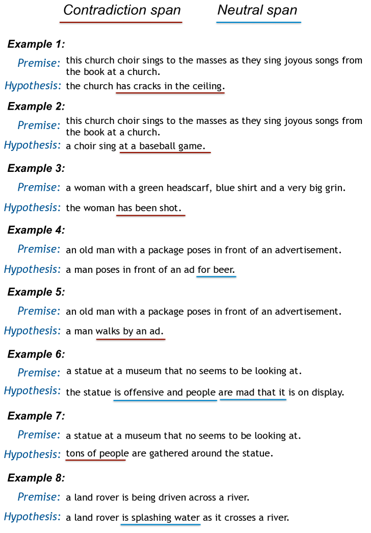
Figure 5: Span and sentence level predictions for the first eight neutral and contradiction examples in SNLI-test. The first example is incorrectly predicted as being contradiction (instead of neutral), while the eighth example is incorrectly predicted as being neutral (instead of entailment). The other predictions are correct and show that the model is making sensible span-level decisions. As the fourth SNLI-test observation is displayed in the main paper we do not repeat this example, and instead we show the ninth example.

Appendix C Hyper-Parameter Choices

We use a BERT-base Devlin et al. (2019) model, providing a direct comparison to previous work. We choose the best learning rate for the baseline, SLR-NLI and SLR-NLI-eSNLI from $\{10^{-6},2.5\times 10^{-6},5\times 10^{-6},7.5\times 10^{-6},10^{-5}\}$. Each SNLI model is trained over 2 epochs, using a linear learning schedule with a warmup and warmdown period of a single epoch. For the SICK dataset, we train with 3 warmup and 3 warmdown epochs with a learning rate of $10^{-5}$ to reach a baseline comparable with previous work. $\lambda^{\text{e-SNLI}}$ is set as 0.1. We also consider spans that consist of up to 3 smaller, consecutive spans. A separate hyper-parameter search is conducted for the reduced data setting, with models evaluated with early stopping across 10 epochs. We also perform an additional hyper-parameter search for the DeBERTa-base model He et al. (2021) and for our SLR-NLI-eSNLI model using this baseline. Each hyper-parameter is tested across 5 random seeds, comparing the mean results.

For the baseline BERT model, we find the best performance using a learning rate of $10^{-5}$, whereas SLR-NLI uses a learning rate of $7.5\times 10^{-6}$ and SLR-NLI-eSNLI uses a learning rate of $5\times 10^{-6}$. For the DeBERTa-baseline, we find the best performance with a learning rate of $7.5\times 10^{-6}$, compared to $2.5\times 10^{-6}$ for SLR-NLI-eSNLI when using DeBERTa.

For each of our experiments in a reduced data setting, the best performance uses a learning rate of $10^{-5}$ for both SLR-NLI-eSNLI and the baseline. We use the same learning rates when training our model on SICK.

References

- Abzianidze (2017) Lasha Abzianidze. 2017. LangPro: Natural language theorem prover. In Proceedings of the 2017 Conference on Empirical Methods in Natural Language Processing: System Demonstrations, pages 115–120, Copenhagen, Denmark. Association for Computational Linguistics.
- Abzianidze (2020) Lasha Abzianidze. 2020. Learning as abduction: Trainable natural logic theorem prover for natural language inference. In Proceedings of the Ninth Joint Conference on Lexical and Computational Semantics, *SEM@COLING 2020, Barcelona, Spain (Online), December 12-13, 2020, pages 20–31. Association for Computational Linguistics.
- Belinkov et al. (2019) Yonatan Belinkov, Adam Poliak, Stuart Shieber, Benjamin Van Durme, and Alexander Rush. 2019. Don’t take the premise for granted: Mitigating artifacts in natural language inference. In Proceedings of the 57th Annual Meeting of the Association for Computational Linguistics, pages 877–891, Florence, Italy. Association for Computational Linguistics.
- Bouchard et al. (2015) Guillaume Bouchard, Sameer Singh, and Théo Trouillon. 2015. On approximate reasoning capabilities of low-rank vector spaces. In AAAI Spring Symposia.
- Bowman et al. (2015) Samuel R. Bowman, Gabor Angeli, Christopher Potts, and Christopher D. Manning. 2015. A large annotated corpus for learning natural language inference. In Proceedings of the 2015 Conference on Empirical Methods in Natural Language Processing, pages 632–642, Lisbon, Portugal. Association for Computational Linguistics.
- Bujel et al. (2021) Kamil Bujel, Helen Yannakoudakis, and Marek Rei. 2021. Zero-shot sequence labeling for transformer-based sentence classifiers. In Proceedings of the 6th Workshop on Representation Learning for NLP (RepL4NLP-2021), pages 195–205, Online. Association for Computational Linguistics.
- Camburu et al. (2018) Oana-Maria Camburu, Tim Rocktäschel, Thomas Lukasiewicz, and Phil Blunsom. 2018. e-snli: Natural language inference with natural language explanations. In Advances in Neural Information Processing Systems, volume 31. Curran Associates, Inc.
- Carton et al. (2022) Samuel Carton, Surya Kanoria, and Chenhao Tan. 2022. What to learn, and how: Toward effective learning from rationales. In Findings of the Association for Computational Linguistics: ACL 2022, pages 1075–1088, Dublin, Ireland. Association for Computational Linguistics.
- Chen et al. (2021) Zeming Chen, Qiyue Gao, and Lawrence S. Moss. 2021. Neurallog: Natural language inference with joint neural and logical reasoning. In Proceedings of *SEM 2021: The Tenth Joint Conference on Lexical and Computational Semantics, *SEM 2021, Online, August 5-6, 2021, pages 78–88. Association for Computational Linguistics.
- Clark et al. (2019) Christopher Clark, Mark Yatskar, and Luke Zettlemoyer. 2019. Don’t take the easy way out: Ensemble based methods for avoiding known dataset biases. In Proceedings of the 2019 Conference on Empirical Methods in Natural Language Processing and the 9th International Joint Conference on Natural Language Processing (EMNLP-IJCNLP), pages 4069–4082, Hong Kong, China. Association for Computational Linguistics.
- Clark et al. (2020) Peter Clark, Oyvind Tafjord, and Kyle Richardson. 2020. Transformers as soft reasoners over language. In Proceedings of the Twenty-Ninth International Joint Conference on Artificial Intelligence, IJCAI 2020, pages 3882–3890. ijcai.org.
- Dagan et al. (2005) Ido Dagan, Oren Glickman, and Bernardo Magnini. 2005. The PASCAL recognising textual entailment challenge. In Machine Learning Challenges, Evaluating Predictive Uncertainty, Visual Object Classification and Recognizing Textual Entailment, First PASCAL Machine Learning Challenges Workshop, MLCW 2005, Southampton, UK, April 11-13, 2005, Revised Selected Papers, volume 3944 of Lecture Notes in Computer Science, pages 177–190. Springer.
- Devlin et al. (2019) Jacob Devlin, Ming-Wei Chang, Kenton Lee, and Kristina Toutanova. 2019. BERT: Pre-training of deep bidirectional transformers for language understanding. In Proceedings of the 2019 Conference of the North American Chapter of the Association for Computational Linguistics: Human Language Technologies, Volume 1 (Long and Short Papers), pages 4171–4186, Minneapolis, Minnesota. Association for Computational Linguistics.
- Efron and Tibshirani (1993) Bradley Efron and R Tibshirani. 1993. An introduction to the bootstrap.
- Feng et al. (2022) Yufei Feng, Xiaoyu Yang, Xiaodan Zhu, and Michael Greenspan. 2022. Neuro-symbolic natural logic with introspective revision for natural language inference. Transactions of the Association for Computational Linguistics, 10:240–256.
- Feng et al. (2020) Yufei Feng, Zi’ou Zheng, Quan Liu, Michael A. Greenspan, and Xiaodan Zhu. 2020. Exploring end-to-end differentiable natural logic modeling. In Proceedings of the 28th International Conference on Computational Linguistics, COLING 2020, Barcelona, Spain (Online), December 8-13, 2020, pages 1172–1185. International Committee on Computational Linguistics.
- Gururangan et al. (2018) Suchin Gururangan, Swabha Swayamdipta, Omer Levy, Roy Schwartz, Samuel Bowman, and Noah A. Smith. 2018. Annotation artifacts in natural language inference data. In Proceedings of the 2018 Conference of the North American Chapter of the Association for Computational Linguistics: Human Language Technologies, Volume 2 (Short Papers), pages 107–112, New Orleans, Louisiana. Association for Computational Linguistics.
- He et al. (2021) Pengcheng He, Xiaodong Liu, Jianfeng Gao, and Weizhu Chen. 2021. Deberta: decoding-enhanced bert with disentangled attention. In 9th International Conference on Learning Representations, ICLR 2021, Virtual Event, Austria, May 3-7, 2021. OpenReview.net.
- Hu et al. (2020) Hai Hu, Qi Chen, Kyle Richardson, Atreyee Mukherjee, Lawrence S. Moss, and Sandra Kuebler. 2020. MonaLog: a lightweight system for natural language inference based on monotonicity. In Proceedings of the Society for Computation in Linguistics 2020, pages 334–344, New York, New York. Association for Computational Linguistics.
- Kalouli et al. (2020) Aikaterini-Lida Kalouli, Richard S. Crouch, and Valeria de Paiva. 2020. Hy-nli: a hybrid system for natural language inference. In Proceedings of the 28th International Conference on Computational Linguistics, COLING 2020, Barcelona, Spain (Online), December 8-13, 2020, pages 5235–5249. International Committee on Computational Linguistics.
- Kalouli et al. (2017) Aikaterini-Lida Kalouli, Livy Real, and Valeria de Paiva. 2017. Textual inference: getting logic from humans. In IWCS 2017—12th International Conference on Computational Semantics—Short papers.
- Kok and Domingos (2007) Stanley Kok and Pedro M. Domingos. 2007. Statistical predicate invention. In ICML ’07.
- Kumar and Talukdar (2020) Sawan Kumar and Partha Talukdar. 2020. NILE : Natural language inference with faithful natural language explanations. In Proceedings of the 58th Annual Meeting of the Association for Computational Linguistics, pages 8730–8742, Online. Association for Computational Linguistics.
- Mahabadi et al. (2020) Rabeeh Karimi Mahabadi, Yonatan Belinkov, and James Henderson. 2020. End-to-end bias mitigation by modelling biases in corpora. In Proceedings of the 58th Annual Meeting of the Association for Computational Linguistics, pages 8706–8716, Online. Association for Computational Linguistics.
- Marelli et al. (2014) Marco Marelli, Stefano Menini, Marco Baroni, Luisa Bentivogli, Raffaella Bernardi, and Roberto Zamparelli. 2014. A SICK cure for the evaluation of compositional distributional semantic models. In Proceedings of the Ninth International Conference on Language Resources and Evaluation (LREC’14), pages 216–223, Reykjavik, Iceland. European Language Resources Association (ELRA).