Transference for loose Hamilton cycles in random -uniform hypergraphs
Abstract
A loose Hamilton cycle in a hypergraph is a cyclic sequence of edges covering all vertices in which only every two consecutive edges intersect and do so in exactly one vertex. With Dirac’s theorem in mind, it is natural to ask what minimum -degree condition guarantees the existence of a loose Hamilton cycle in a -uniform hypergraph. For and each , the necessary and sufficient such condition is known precisely. We show that these results adhere to a ‘transference principle’ to their sparse random analogues. The proof combines several ideas from the graph setting and relies on the absorbing method. In particular, we employ a novel approach of Kwan and Ferber for finding rooted absorbers in subgraphs of sparse hypergraphs via a contraction procedure. In the case of , our findings are asymptotically optimal.
1 Introduction
The question of deciding when a given graph is Hamiltonian is in general notoriously difficult and was included in Karp’s original list of 21 NP-complete problems [34]. Being a fundamental problem in graph theory (and computer science), Hamiltonicity has inspired a long line of work exploring sufficient conditions for it. Perhaps the best known among those is the classical theorem of Dirac [14]: every graph on vertices with minimum degree at least contains a Hamilton cycle. Another regime in which the problem is understood better than in the general case is that of random graphs (also, more broadly, quasi-random graphs and expanders). In that regard, Pósa [59] and independently Korshunov [43] proved that if , for some constant , then the Erdős-Rényi binomial random graph 111 stands for a graph on vertices in which each edge exists with probability independently. is with high probability222With high probability (or w.h.p. for brevity) means with probability going to as tends to infinity. Hamiltonian. The more precise value for which the former holds was later determined by Komlós and Szemerédi [42], and an even stronger, so-called hitting-time result, was shown by Ajtai, Komlós, and Szemerédi [1] and independently by Bollobás [7].
Inquiring further into properties of random graphs, Sudakov and Vu [63] asked how resilient is with respect to having a Hamilton cycle. A graph is -resilient with respect to a property if after the removal of at most an -fraction of edges incident to every vertex of , the resulting graph (still) contains . Observe that Dirac’s theorem states exactly that: the complete graph on vertices is -resilient with respect to Hamiltonicity (with being optimal as witnessed by two disjoint cliques of size ). The work of Sudakov and Vu initiated a systematic study of minimum degree requirements in the flavour of Dirac’s theorem for random graphs as they showed that for , w.h.p. is -resilient with respect to Hamiltonicity. A full analogue of Dirac’s theorem for random graphs was later established by Lee and Sudakov [51]: if then w.h.p. is -resilient with respect to Hamiltonicity. Even more, the absolutely best-possible hitting-time results were recently obtained by Montgomery [52] and independently Nenadov, Steger, and the second author [56].
There are, however, certain deficiencies of the basic notion of resilience in the usual binomial random graph—for example, it is unable to capture the behaviour of with respect to containment of large structures riddled with triangles. Namely, as soon as , one can easily prevent as many as vertices from being in a triangle while removing only edges incident to each vertex (see [3, 31]). This makes the study of resilience for, e.g., a triangle-factor or any power of a Hamilton cycle futile. Recently, Fischer, Steger, Škorić, and the second author extended the notion of resilience to -resilience in order to study robustness of with respect to the containment of the square of a Hamilton cycle [21]. Roughly speaking, they determined the smallest such that, for , w.h.p. every in which every vertex belongs to at least triangles contains the square of a Hamilton cycle.
Such a concept naturally corresponds to resilience in hypergraphs, with the added advantage that edges in a random hypergraph are independent, unlike copies of in . Thus, the hypergraph counterpart to the questions above can be a solid test case for developing new ideas and techniques. Of course, studying resilience of Hamiltonicity in hypergraphs is also of independent interest as a natural ‘high-dimensional’ generalisation of one of the most important questions in graph theory to a radically more challenging setting.
In this paper, we are concerned with Dirac-type conditions, hence resilience, for Hamiltonicity in random -uniform333A hypergraph is -uniform, also called -graph for short, if every edge consists of exactly vertices. hypergraphs. The notions of cycles and degrees do not generalise unambiguously to the hypergraph setting, so in what follows we make them more specific. For some , an -cycle in a -graph is a cyclic sequence of edges such that each two consecutive edges overlap in exactly vertices, and no pair of non-consecutive edges have vertices in common. The most studied special cases are and , which are referred to as a loose and a tight cycle, respectively. Note that the number of vertices in any -cycle is necessarily divisible444From now on, we always assume that the hypergraph we are dealing with has its number of vertices divisible by the appropriate integer needed for a loose Hamilton cycle to exist. by . In a -graph , for some , the -degree of a -element set of vertices is the number of edges such that . The -degree of a vertex is referred to simply as its degree, and the -degree of a -set as its codegree. The minimum -degree of is the minimum value among the -degrees over all -sets .
As is the case with graphs, there is a large body of research studying various Dirac-type conditions in hypergraphs, that is smallest -degree which implies existence of Hamilton -cycles (e.g. [60, 61, 46], surveys [49, 64] and the references within). Most closely related to the present work, for , Keevash, Kühn, Mycroft, and Osthus [36] and independently Hán and Schacht [28] showed that every (sufficiently large) -vertex -graph with contains a loose Hamilton cycle, which is asymptotically optimal (up to the term). In case of -graphs, it was previously known that implies (loose) Hamiltonicity, with for or for (see [10, 47] and their strengthening [29, 13]). Neither of the values can be improved upon.
When it comes to (sparse) random structures, Dudek, Frieze, Loh, and Speiss [15] showed that 555 stands for the (random) graph on vertices in which each set of vertices is chosen as an edge independently with probability . w.h.p. contains a loose Hamilton cycle, provided that (this generalises a previous result of Frieze [22]; see also [17] for a short proof and [58] for a much more general framework from which this follows directly). This result is asymptotically optimal, since for of lower order of magnitude, w.h.p. has isolated vertices.
Our main contribution is a resilience variant of this result for -graphs, thus transferring the formerly mentioned Dirac-type statements to the sparse random setting.
Theorem 1.1.
Let . For every there is a such that the following holds. Suppose and is even. Then w.h.p. has the property that every spanning subgraph with contains a loose Hamilton cycle.
The constants and are optimal—in other words, w.h.p. there exists a subgraph of with minimum -degree which does not have a loose Hamilton cycle. One can see this by, e.g., considering analogues of dense extremal constructions from [10] (in case ) and [47] (in case ).
The more interesting part are the limitations for the density . Observe that one can more concisely summarise the density requirements as , however we chose to present them separately to underline their distinct origins. In case , if for some small , then w.h.p. contains pairs of vertices with -degree equal to zero, and thus Theorem 1.1 is optimal (up to the multiplicative constant). However, the bound for is ‘artificial’ but crucial for our proof technique. It is highly likely, but probably quite challenging to prove, that the result should remain true all the way down to —the threshold for appearance of a loose Hamilton cycle in . It seems that one would need to explore completely different techniques in order to establish this.
Note that this provides a resilience result for with respect to containment of a loose Hamilton cycle—it shows that is -resilient for this property (similarly one can think of ‘codegree resilience’ in terms of ). This partially answers a question raised by Frieze [23, Problem 56] in his survey on Hamilton cycles in random graphs. Being only the beginning of the story, a natural next step would be an extension to hypergraphs of larger uniformities. One obstacle on the way is that the corresponding dense Dirac condition with is not known for -graphs with (a ‘transference’ result could be obtained even without knowing this value, see [20]). In addition, our methods do not seem to straightforwardly generalise to regardless of the type of degree considered.
Usually, establishing properties of hypergraphs is substantially more difficult than in the case of their graph counterparts, hence it is not surprising that not much is known about resilience of random hypergraphs. Prior to this, Clemens, Ehrenmüller, and Person [11] studied resilience of with respect to the containment of a Hamilton Berge cycle, and, very recently, Allen, Parczyk, and Pfenninger [2] proved that is resilient for containment of tight Hamilton cycles. On a related note, Ferber and Kwan [20] proved a very general ‘transference principle’ concerning perfect matchings in random -graphs (see also [18] for a specific result when ).
On the whole, our proof follows a standard strategy for embedding relying on the absorbing method. In a nutshell, this method allows one to reduce the problem of finding a spanning structure to the usually significantly easier one of finding an almost-spanning one. For the latter we combine several ideas originating from their graph counterparts such as the DFS technique for finding long paths (Section 4), path connection techniques (Section 5), and the sparse regularity method (Section 3). As always, the most difficult, involved, and creative part comes in designing and finding the absorber (see Definition 6.1 below). The ‘finding’ part is partially done through a contraction procedure of Ferber and Kwan which helps with finding absorbers inside a regular partition of . We discuss this, as well as the absorbing method in general, in much greater detail in Section 6. All these ingredients are mixed together following a usual recipe to give a proof of Theorem 1.1 (Section 7).
2 Preliminaries
Our graph theoretic notation mostly follows standard textbooks in the area, e.g. [8]. More specifically, for a (hyper)graph we let and denote the number of its vertices and edges, respectively. Given a set of vertices , stands for the induced graph . For sets we let denote the number of triples for which . Instead of , we write for brevity. Similarly, if is a set of pairs of vertices, then counts the number of (ordered) pairs for which with and . For a set , we use , respectively , for the number of distinct pairs with , respectively the number of vertices , for which . The neighbourhood of a vertex in a set refers to the set of vertices such that for some , and we denote as for brevity. Similarly, the neighbourhood of a pair of vertices in a set denotes the set of vertices with , and we abbreviate to .
A loose path of length is an ordered sequence of distinct vertices and edges: for all . Note that a loose path always consists of an odd number of vertices. Throughout, whenever we say path we mean loose path and we write -path for a path whose start- and end-points are and . A (loose) cycle is defined similarly.
All logarithms are in base . For , stands for the set of first integers, that is . We use standard asymptotic notation , and . For a set and an integer , denotes the collection of all -element subsets, -sets for brevity, of , and denotes the collection of all distinct -tuples with and for each . When using set-theoretic notation, we treat tuples as corresponding sets, e.g. stands for and two tuples are disjoint if they do not share an element.
2.1 Distribution of edges
In this subsection we list some lemmas that give upper bounds on the number of edges between various vertex sets in .
Lemma 2.1.
For every and there exists such that w.h.p. satisfies the following, provided that . There are no two disjoint sets of sizes and such that , , and .
Proof.
Set . Fix , , and two disjoint sets and of sizes and , respectively. The probability that is at most
This is at most provided is chosen small enough with respect to and . Then the union bound over at most choices for the sets and completes the proof. ∎
Lemma 2.2.
For every , w.h.p. satisfies the following. Let be sets of size and .
-
(i)
If then .
-
(ii)
If then .
Proof.
Let . The probability that there exist , of sizes for which is at most
If , from Chernoff’s inequality (see, e.g. [32, Corollary 2.3])
Then by the union bound, the probability that the property of the lemma fails is at most
once again. ∎
Proving the next two lemmas follows similar steps as for the one above, using a straightforward application of Chernoff’s inequality and the union bound. Thus, we omit the proofs.
Lemma 2.3.
For every , w.h.p. satisfies the following. Let and .
-
(i)
If then .
-
(ii)
If then .
Lemma 2.4.
For every , w.h.p. satisfies the following. Let be (not necessarily disjoint) sets of size , , , such that . Then
In particular, if , then .
2.2 Expansion
The following lemma captures the fact that expansion of vertices behaves as expected in a not too sparse subgraph of the random graph . Namely, if a vertex has the property that for some the minimum degree of is at least , then there are at least vertices and vertices for which there is a -path of length in . It plays an important role both for proving the Connecting Lemma and finding absorbers.
Lemma 2.5.
For every there exist such that w.h.p. satisfies the following, provided that . Let and with . For every for which , there exist and , all pairwise disjoint, of size , , and such that
-
(A1)
, for every , and
-
(A2)
for every there is some for which .
Proof.
Suppose has the properties of Lemma 2.2 and Lemma 2.4 for, say, . Let be a maximal set of disjoint pairs which close an edge together with , and suppose . Let be a superset of all the vertices that belong to these pairs of size precisely . Then, in particular, there are no edges with . Note that by our choice of for large enough. From the minimum degree assumption on the one hand, and the property of Lemma 2.2 on the other, we have
This is a contradiction for large enough.
Similarly, after fixing and , let be a maximal set of disjoint -tuples which satisfy the second property of the lemma, and suppose . Let be the vertices that belong to these -tuples. We first show there is a set of size such that for every there exist distinct (also from other such vertices) which close an edge in with . Let be the largest such set and let denote the union of and all such (the ones that closes an edge with). Then, with denoting the vertices in , we have
On the other hand, by the property of Lemma 2.2, assuming and as (taking a superset if necessary), we have
leading to a contradiction for small enough. We just need to show that there is and which comprise an edge in with . Indeed, exactly the same computation as above establishes this, which completes the proof. ∎
2.3 Degree inheritance properties
We first state a slightly strengthened version of [20, Lemma 5.5]. The strengthening comes in the bound on , which is stated to match the one from Theorem 1.1 (and in fact, most of the statements in this paper). For the case we require , in contrast to , and here the desired property is in fact easily obtained through Chernoff’s inequality and the union bound due to independence. In case the former requirement of is actually necessary for this particular proof.
Lemma 2.6.
For every , there is a such that w.h.p. satisfies the following, provided that . Let and let be a uniformly random set of size at least . Then w.h.p. every -set that satisfies also satisfies .
Proof.
For , the codegree of a pair of vertices into follows a hypergeometric distribution with mean , for which Chernoff’s inequality applies (see, e.g. [32, Theorem 2.10]). The statement thus follows directly from it and the union bound over all pairs of vertices. In case the assertion holds by [20, Lemma 5.5], since . ∎
The next lemma allows us to start with a graph in which almost all -sets have at least some degree and pick a random subgraph of it such that in it, with positive probability, all -sets have at least some (slightly smaller) degree.
Lemma 2.7 ([20, Lemma 3.4]).
There is a such that the following holds. Let and . Let be an -vertex -graph in which all but of the -sets have degree at least . Let be a uniformly random subset of vertices of . Then with probability at least , the random induced subgraph has minimum -degree at least .
The last two lemmas establish that in a subgraph of the random hypergraph with sufficiently large minimum degree, after an adversary removes vertices, for some tiny , almost all -sets still keep a significant portion of their original degree in the resulting graph.
Lemma 2.8.
For every there exist such that w.h.p. satisfies the following, provided that . Let with and let be of size . Then there exists a set of size at most such that for , the graph is of minimum degree at least . Furthermore, if for some we have , then can be chosen to avoid .
Proof.
Initially, let . As long as there exists and with
add such a vertex to . Stop this process at the first point in time when , for some small enough . Note that by the assumption on , it also holds that . We then have
On the other hand, as w.h.p. satisfies the conclusion of Lemma 2.2,
which is a contradiction with the former, for small enough.
Consider now and its degree into . If it does not satisfy the bound promised by the lemma, this means
On the other hand, again by the property of Lemma 2.2,
This is a contradiction with the former for large enough as by the assumption on . ∎
Lemma 2.9.
For every , there exist such that for every w.h.p. satisfies the following. Let with . Then, for every with , all but at most pairs of vertices have .
Proof.
Let
As w.h.p. has the property of Lemma 2.3 for , assuming we have
This leads to a contradiction for sufficiently small and large enough, as and . ∎
2.4 (Hyper)graph theory
The following Dirac-type conditions for the existence of a loose Hamilton cycle were mentioned in the introduction but we state them here explicitly in the form in which we use them later. Recall, and .
Theorem 2.10 ([10, 47]).
Let and . Every sufficiently large -uniform hypergraph on an even number of vertices with contains a loose Hamilton cycle.
The next lemma gives a minimum degree condition for a 3-graph that ensures that any pair of vertices is contained in some loose cycle of length 3. We make use of it later for finding absorbers.
Lemma 2.11.
Let be a sufficiently large -vertex -uniform hypergraph which satisfies . Then for every pair of vertices , there exist distinct vertices such that .
Proof.
Suppose is a sufficiently large -vertex -graph with , for some . A simple counting argument (see, e.g., [10, Claim 9]) shows that for every two , there is a set of size , such that either:
-
•
and for all , or
-
•
and for all .
Since for , by the discussion above there is a such that, without loss of generality, and for all . Pick an arbitrary and an arbitrary such that . Note that and due to the minimum degree condition for . Therefore, since , we have (with plenty of room to spare). Pick and pick . ∎
We lastly need a Hall-type matching condition for ‘bipartite’ hypergraphs due to Haxell, which has been used frequently for embedding problems in random graph theory.
Theorem 2.12 (Haxell’s condition [30]).
Let be an -hypergraph, where the vertex set can be partitioned into sets and such that , and . Suppose that and such that , there exists an edge with but . Then has an -saturating matching (i.e. a collection of disjoint edges whose union contains ).
3 The sparse regularity method for hypergraphs
Following [20, 19] in a natural generalisation of the analogous concept for graphs, we say that, given and , a -partite -graph on sets is -regular if for every , , we have
where stands for the density of edges of a given triple.
A partition of the vertex set of a -graph is said to be -regular if it is an equipartition and for all but at most triples , the graph induced by them is -regular. For the (hyper)graph regularity lemma to be of any use, it usually needs to prevent too many edges lying within some partition class . A common way to restrict this is the notion of upper-uniformity. We say that a -graph is -upper-uniform, for some and , if for all disjoint sets with .
With all these concepts at hand, we state a so-called weak666‘Weak’ comes from the fact that in this variant, the corresponding counting and embedding lemmas are not necessarily true in general—one would require a stronger concept of regularity. hypergraph regularity lemma, which acts as a natural generalisation from the graph setting, can be proven in the same way (see, e.g. [38, 41, 25] for the sparse regularity lemma and [40] for the regularity lemma in dense hypergraphs), and appears in the same form in [20, 19].
Theorem 3.1.
For every and there exist and such that for every , every -upper-uniform -graph with at least vertices admits an -regular partition , where .
The upper-uniformity property can be seen as a ‘true property of random graphs’ and indeed is exhibited by with high probability (e.g. established by a straightforward application of Chernoff’s inequality and the union bound).
Lemma 3.2.
For every and the random -graph is -upper-uniform with probability at least , provided that .
Given an equipartition of the vertex set of a -graph , we define the reduced graph on vertex set corresponding to the sets , whose edges are all -element sets of indices such that and is -regular.
In fact, in the regularity lemma, one can even roughly define where the clusters lie in the graph . Namely, given a partition , the -regular partition resulting from Theorem 3.1 can be made such that all but at most clusters each completely belong to one (may be distinct for different ). This comes in handy when it comes to finding absorbers.
The property that we use most frequently is that the reduced graph in a way inherits degree properties from its underlying graph . This is nothing fancy and should come as no surprise to anyone familiar with the (graph) regularity method. Again, very conveniently, one can make it such that degrees are ‘controlled’ within certain predetermined sets, and not only globally in the whole graph . The following statement is almost a one-to-one copy of [20, Lemma 4.7] (slightly paraphrased for convenience).
Lemma 3.3 ([20, Lemma 4.7]).
For all and , there exist such that the following holds. Let and let be a sufficiently large -vertex -upper-uniform -graph. Let and be a partition of with . Then there exists an -regular partition of , for some and a corresponding reduced -vertex -graph with the following property. Let be the set of clusters contained entirely in and let . Then:
-
(i)
for every .
-
(ii)
Let . Suppose that for some all but at most of the -sets satisfy
Then all but at most of the -sets satisfy
We remark that, if one wants to only inherit minimum degree (that is, ), then standard double counting methods (see e.g. [57]) show that this can be done without having the error term. Namely, actually all vertices satisfy the corresponding degree assumption. For , the ‘almost all’ is necessary.
Lastly, we use a hypergraph version of the infamous KŁR conjecture777still known by this name, but has since its introduction [39] been proven [4, 62]; for a very recent, short, and self-contained proof see [55]. whose proof for linear hypergraphs was explicitly spelled out in [19] but already observed to hold in the work of Conlon, Gowers, Samotij, and Schacht [12]. For a -graph on vertex set we denote by the class of graphs obtained in the following way. The vertex set of is a disjoint union of sets of size . For each edge we add to an -regular -graph with edges between the triple (and these are the only edges of ). A canonical copy of in is a -tuple with for every and for every . We write for the number of canonical copies of in . Lastly, we need the notion of -density of a -graph , which is defined as
Theorem 3.4.
For every linear -graph and every , there exist with the following property. For every , there is a such that if , then with probability the following holds in . For every , , and every subgraph of in , we have .
Strictly speaking, the subgraph that we later apply Theorem 3.4 to is not a member of , in particular not all -regular 3-graphs have exactly edges—the number of edges across these are within a constant factor of each other. However, subsampling (see, e.g. [25, Lemma 4.3]) circumvents this. For clarity of presentation, we prefer to not explicitly spell out this argument.
4 Covering random hypergraphs by loose paths
In this section we show a vital part of every strategy relying on the absorbing method which in our specific problem reads as: the majority of vertices of can be covered by a few (loose) paths. For the purposes of this lemma, we consider single vertices to be loose paths of length zero.
Lemma 4.1.
Let . For every , there exists a such that w.h.p. has the following property, provided that . Let in which all but -sets satisfy . Then there exist at most vertex-disjoint loose paths that cover the vertex set of .
To a reader familiar with the topic, there is no magic that happens here. We apply the sparse regularity lemma to , find a desirable structure in the obtained reduced graph, and then use it as a guide to construct loose paths in itself. Perhaps the most innovative thing comes in the part where, in an -regular triple , we find a long loose path covering all but vertices in each . This itself relies on a widely-used Depth-First Search (DFS) technique employed explicitly in the context of graphs in [5, 6]. (For an extremely neat application of the method and more in-depth discussion see [45].)
Lemma 4.2.
Let be a -partite -graph with and such that for every choice of size , there exists an edge in . Then there is a loose -path of length in with , and whose every other degree-one vertex lies in .
Proof.
We explore the graph by using a variant of the Depth-First Search (DFS) procedure as follows. To start with, set , , and . For as long as , do:
-
•
if , pick an arbitrary vertex from and add it to ;
-
•
if and there is an edge such that is the last added vertex to , and and , move from to in that order;
-
•
otherwise, for being the last three vertices added to , move from to (if there is no such edge just move the only vertex in to ).
Observe that the vertices in at all times span a loose path as wanted in the lemma, but maybe not of the required length, and, crucially, there is never a time when some edge is such that , , and , for . We aim to show that at some point we have which is sufficient for the lemma to hold.
In every step of the procedure either one (if , say) or two vertices get moved from to or from to . Consider the first moment in time when , for some ; we may safely assume this happens for . So, , and moreover by the description of the procedure above, at this point we necessarily have .
As , it cannot be that , by the property of the lemma that such three sets must contain an edge. Assuming , we have as desired.
Otherwise, suppose and . From the fact that we conclude that the intersections of and with are the same (up to ). This further implies (recall, ). Putting things together, we have , and hence again as desired. ∎
As a reminder, the exact values of are known for -uniform hypergraphs to be and .
Proof of Lemma 4.1.
Take sufficiently large and sufficiently small, in particular so that and is small enough, namely . Pick large enough so that . Let , , and .
Since , by Lemma 3.2 is w.h.p. -upper-uniform, and so is then. Therefore, we can apply Lemma 3.3 to with (as ), to obtain an -regular partition for some and a corresponding reduced graph . In particular, we get that for all but at most -sets , it holds that . Let us remove from each at most two vertices to get that they are all of even size (with slight abuse of notation we still refer to them as ).
Let be a partition of into disjoint subsets of size , chosen uniformly at random. Recall that . By Lemma 2.7, with positive probability all but a -fraction of the subgraphs have minimum -degree at least . As we have picked to be even and large, each with this minimum degree has a loose Hamilton cycle by Theorem 2.10. The vertices not covered by loose cycles in are then at most . We next show how to cover each loose cycle in with not too many loose paths in .
Consider a (loose) Hamilton cycle in some and suppose without loss of generality that the clusters corresponding to the vertices of are in the order in which they appear on the cycle. Then we know that is -regular with density at least , for every , odd ( is identified with ). Split every , for odd, arbitrarily into , each of size . By the definition of a regular triple, for all , , and , each of size , we have
and in particular . Lemma 4.2 implies there is a loose -path in with , which is of length and thus uses all but at most vertices in .
Repeating this for every odd , we get loose paths covering all but at most vertices in . The whole thing can independently be repeated for every as well. In total, and counting vertices as paths of length zero, we found at most
loose paths that cover the vertex set of . ∎
5 Connecting Lemma
In this section we prove a vital ingredient both for constructing absorbers and independently as a part of the proof of Theorem 1.1. Roughly speaking, we show that one can connect prescribed pairs of vertices with short paths through a set of vertices under some degree assumptions. Given a set in a graph , an integer , and a set of pairs from , a -matching is a collection of internally vertex-disjoint paths , where each is of length at most , has as endpoints, and its remaining vertices belong to .
Lemma 5.1 (Connecting Lemma).
Let . For every there exist such that w.h.p. satisfies the following, provided . Let and be disjoint subsets such that
-
•
,
-
•
all -sets , have .
Then, for every family of distinct pairs in such that and every appears in at most two pairs, there exists a -matching in .
Proof.
Given and , let be sufficiently small and sufficiently large for the arguments below to go through. Condition on having the properties of Lemma 2.2, Lemma 2.3, Lemma 2.4, Lemma 2.5 for (as ), and Lemma 2.6, which happens with high probability.
Consider an auxiliary -graph with vertex set in which, for , , an edge exists if and only if there is a -path whose all internal vertices belong to . Hence, a -saturating matching in corresponds to a -matching in . Our plan is to use Haxell’s matching theorem (Theorem 2.12) to show this graph indeed contains a -saturating matching. We treat the cases and separately, starting with .
Codegree, .
Recall, . It is sufficient to show that for every and of size , there is an and an edge with . Let be a maximal set of pairs with and all vertices distinct and assume towards a contradiction there are no such edges. By the assumption of the lemma we have . If , using on the one hand the minimum codegree assumption and on the other the property of Lemma 2.3 we obtain
which is a contradiction for large enough, as . Otherwise, if , then again by the property of Lemma 2.3
by taking a superset of of size , leading to a contradiction as .
Degree, .
Recall, . Let be an equipartition of in which each , for , satisfies
| (1) |
for all . From the assumptions of the lemma, it is straightforward to show that such a partition exists by making use of the property of Lemma 2.6 and the union bound.
Consider any and of size . Assume that contains indices so that the collection consists of distinct vertices (a maximal subset of such comprises at least a third of the original which has no influence on the proof). We aim to find an and a -path whose all internal vertices belong to . In particular, the path we find is going to be such that it intersects each in exactly two vertices, and in exactly three vertices. So, fix and as above and set . It is sufficient to show that there is an index for which:
-
(B1)
There exist and , both of size ;
-
(B2)
Let and be auxiliary graphs on the same vertex set and if form an edge in with a vertex from , . Then for each
Before proving these statements, let us show how to complete the proof. If we were to find three vertices so that and , this would close a -path as desired. A path of length two in with one edge in each of corresponds exactly to a triple as above. By (B2) and the pigeonhole principle, there must be a with . This implies we can choose as one of ’s neighbours in and as one of ’s neighbours in such that .
We first show there is an for which (B1) holds. For this, it is sufficient to show that more than half indices are such that . The existence of and the corresponding sets and as in (B1) follows from the pigeonhole principle and the property of Lemma 2.5.
Let be a set of vertices , , with and suppose . Owing to the assumption on the minimum degree (1) this means
| (2) |
If , then the property of Lemma 2.2 implies
Otherwise, if then by the property of Lemma 2.2 again
where we take a superset of or of size exactly if necessary. This again leads to a contradiction with (2) since and by our choice of (with room to spare).
For (B2), let
Assume for contradiction . Note that, by the property of Lemma 2.4 and taking a superset of of size if necessary,
| (3) |
By (1) and for sufficiently small, we thus get
| (4) |
On the other hand, noting that , by the property of Lemma 2.3 and taking supersets of and if necessary,
and so by the property of Lemma 2.4 again
which is smaller than by our choice of , thereby contradicting (4). ∎
6 The absorbing method in sparse hypergraphs
The absorbing method was initially explicitly introduced by Rödl, Ruciński, and Szemerédi [61] even though the implicit idea has its roots in the works of Krivelevich [44] and Erdős, Gyárfás, and Pyber [16]. Recently it has seen a surge of interest and has been used in a variety of settings: combinatorial designs [27, 35], decompositions [26, 48], Steiner systems [50, 19], Ramsey theory [9, 37], colouring (hyper)graphs [54, 33], embeddings [53, 24], and many, many more.
In principle, the idea behind it is simple. It relies on reducing the problem of finding a spanning subgraph in some graph to the one of finding an almost spanning subgraph , say, one of size . Often times, the latter is significantly easier to solve, if nothing else, just for the fact that we have quite a bit of room for error. In practice, the implementation of this idea typically depends on first embedding a highly structured graph into , which is capable of extending any partial embedding to a complete one. The task of designing the graph with this magical property is where the whole art of absorption lies in. Usually, it specific to the embedding problem at hand and is where the main difficulties arise—it can be, first, quite surprising that such a graph should even exist and, second, challenging to find it in the host graph in a convenient way (or in any way for that matter).
When dealing with paths, the ‘design’ of the graph is not too complex. We make this more rigorous.
Definition 6.1 (-absorber).
An -absorber is a graph with , , with the property that for every with such that has odd cardinality, there is a loose -path in with vertex set .
The next lemma handles the second step of the method: actually finding the graph in the subgraph of the random graph .
Lemma 6.2 (Absorbing Lemma).
Let . For every there exist such that w.h.p. has the following property, provided that . Let with . Then, for a uniform random set of size , w.h.p. there exists an -absorber in of order at most .
It may seem awkward that there are two probabilistic statements in the lemma. Indeed, the first w.h.p. establishes some typical properties a random -uniform hypergraph has (such as, e.g., distribution of the edges), whereas the second w.h.p. is over the choice of . Namely, once we condition on having these ‘nice’ properties, then for a randomly chosen set there is an absorber with high probability. In fact, the lemma could be written in a quantitative form, saying how w.h.p. in there are at least, say, a -fraction of choices for which yield an absorber. We found this a bit more cumbersome to deal with and decided to go with the former.
As per usual, the ‘construction’ of such a graph consists of carefully patching up many small structures.
Definition 6.3 (-absorber).
An -absorber rooted at two vertices is a graph that consists of:
-
•
a path , which we refer to as the covering path, and
-
•
a path , which we refer to as the non-covering path, with and whose endpoints are identical with those of .
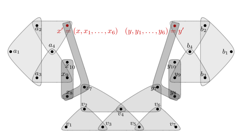
We now define the -absorber we use, depending on (in doing this we draw inspiration from [10]). Both of these, however, have a much more natural visual representation depicted in Figure 2 and Figure 1.
Definition 6.4.
The -absorber rooted at a pair of vertices is defined as:
-
()
consists of nine vertices , and the edges , , , , .
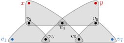
Figure 1: The -absorber rooted at . -
()
consists of:
-
•
a cycle , where is an -path of length ;
-
•
a cycle , where is a -path of length ;
-
•
a copy of rooted at ;
-
•
edges , , and , , ;
-
•
an -path and a -path, both of length .
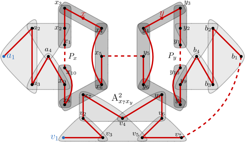
(a) The covering -path 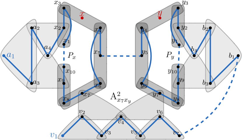
(b) The non-covering -path Figure 2: The -absorber rooted at . The dashed lines represent paths of length four. -
•
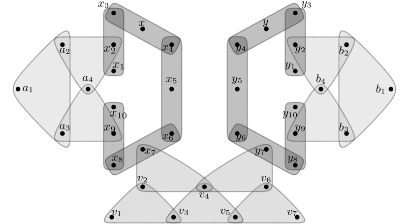
For future reference, the graph obtained by removing , , the -path, and the -path is called a backbone of the -absorber (see Figure 3(a) below).
To build an -absorber, we plan to string together a number of copies of . Clearly, we cannot just build disjoint -absorbers for every pair of vertices for the simple reason of there not being enough space for that as . A way of dealing with this originated in the work of Montgomery [53], who used an idea of looking at an auxiliary bounded degree graph, which serves as a template for which pairs of vertices of to use. Roughly speaking, there is a graph on the vertex set and with , so that if for every we find disjoint -absorbers, then the obtained graph is an -absorber, for some .
The following lemma is very similar to [20, Lemma 7.3], but it has the additional property that the template graph it describes has bounded maximum degree. The proof, being almost identical to that of the mentioned lemma, is for completeness spelled out in the appendix.
Lemma 6.5.
There is an such that the following holds. For any sufficiently large , there exists a graph with , maximum degree at most , and a set of vertices, such that for every with and even, the graph has a perfect matching.
At this point, we essentially reduced our goal to finding a single -absorber rooted at a prescribed pair of vertices . This is the key lemma of this section.
Lemma 6.6.
Let . For any there exist , such that w.h.p. satisfies the following, provided that . Let with and let with . For any two , which if necessarily satisfy , there exists a copy of in .
We remark that the degree assumption for is not needed in the case. The proof of this lemma is the most intricate part of the argument so we defer it to Section 6.1. With all these ingredients we can now prove the absorbing lemma.
Proof of Lemma 6.2.
Let denote the number of vertices in and further set
Having chosen these, let be sufficiently small with respect to all constants (in particular, small with respect to the given ) and sufficiently large. Write and let be the auxiliary graph given by Lemma 6.5 for . Assume is such that it satisfies the conclusion of Lemma 2.1 with (as ) and (as ), Lemma 2.6, Lemma 5.1, and Lemma 6.6 with (as ).
Choose a uniform random set of size and let be a partition of such that:
-
(C1)
, , and ;
-
(C2)
, for every -set and .
Note that, in particular, . By the property of Lemma 2.6 almost any choice of such a partition will do.
Let be a bijection which maps the vertices belonging to the set in to . For each edge , we plan to first find an -absorber whose internal vertices belong to in such a way that all these absorbers are pairwise internally vertex-disjoint. Subsequently, we string all the -absorbers together by an application of the Connecting Lemma (Lemma 5.1) over the set .
The first part of this is to be completed using Haxell’s condition and Lemma 6.6. Let be a -uniform hypergraph with vertex set , where . For and with , we add the edge to if and only if there is a copy of in . Then what we are looking for is precisely a -saturating matching in . Comparing to Haxell’s condition (Lemma 2.12), it is sufficient to show that for every and with , there is some and a copy of in whose internal vertices are fully contained in .
As , we can greedily find a set of pairwise vertex-disjoint edges for which and which is of size at least . For simplicity, we assume already consists only of such disjoint edges—this changes nothing in the proof. In case , straightforwardly applying Lemma 6.6 with any for which (as ), (as ), and (as ), we are done. Note that we can indeed do so since
In the other case, , the only thing remaining is to check that there are with that satisfy the degree requirement . Towards contradiction, suppose there is no such . Let be the union of all that violate the prior requirement and such that for some , , and assume . On the one hand, this means
while on the other, by the property of Lemma 2.1 since and ,
which is a contradiction. So, and by the pigeonhole principle, there has to exist a pair with the desired degree value into .
Finally, we use Lemma 5.1 to connect all -absorbers into one loose path. Denote the absorbers we have found as , for , each a copy of . We want to, for every , connect and if (see Figure 2) and and if (see Figure 1). Let be the set of (the images of) all these vertices we would like to connect. We use the property of Lemma 5.1 with , (as ) which we can do by (C2) and since and the total number of pairs we want to connect with paths is
Lastly, observe that the total number of vertices used by this whole procedure is
as desired.
It remains to establish that the graph we obtain comprises an -absorber, where and are (the images of) and if and (the images of) and if . Namely, let of size be such that has odd cardinality. Note that must also be of odd cardinality as it can be covered by a loose path (by taking the non-covering paths of all individual -absorbers) and hence, crucially, is of even cardinality. In particular, this means there is a perfect matching for in . Consider the set of -absorbers corresponding to the edges in this matching. Then, as a witness for the absorbing property of , we can use the covering path for all these absorbers and the non-covering path for all other -absorbers. ∎
6.1 Finding an -absorber robustly
In this section we prove Lemma 6.6. The case is much simpler, so we deal with it first.
Proof of Lemma 6.6 for .
We use the property of Lemma 2.9 to get a set of size (by choosing sufficiently large) such that all pairs satisfy , for . Recall, our goal is to find a copy of rooted at in (see Figure 1).
Since is relatively small, there must be some such that neither nor belong to . Having chosen , take distinct such that are edges in . Let
and
and note that and . It is enough to show that there is an edge in such that and , because imply that we can choose and as desired for .
Suppose for contradiction such an edge does not exist in . Then, from the codegree assumption and the property of Lemma 2.4, we have
which is a contradiction. Thus, an edge exists as desired. ∎
In what follows we provide a proof of Lemma 6.6 for . This is the most involved part of the whole proof and we, for convenience of reading, first give a brief outline. The main idea relies on an intricate combination of the sparse regularity method and the connecting lemma. It consists of two almost independent steps: (1) find a backbone of an absorber rooted at ; (2) use the Connecting Lemma (Lemma 5.1) to find the remaining loose paths which comprise an absorber (see Figure 2). Most of the difficulty lies in the first part. To do this, we use the ‘contraction technique’ of Ferber and Kwan [20] and the regularity method. In order for the next steps to make more sense, we first introduce a definition.
Definition 6.7.
A contracted absorber backbone rooted at a pair of vertices , is a graph that consists of:
-
•
edges , and , , ;
-
•
edges , and , , ;
-
•
a copy of rooted at ;
A contracted absorber backbone can be thought of as starting with and contracting the edges into a single vertex , and keeping only the edges ‘to the outside’ (that is, ones containing or ). The same is done to obtain . For a more natural visual representation we depict this contraction operation below.
The contraction operation on , almost analogous to the one of Ferber and Kwan, is defined as follows. For a -graph , a collection of disjoint sets , and a family of disjoint -tuples we let be a -graph on vertex set and whose edge set is given as follows: add first all edges from and next, for every , we add an edge to if and only if and or and .
We can now continue with the outline. Namely, imagine for a moment that we can find a collection of distinct -tuples such that, , for some . Let us, for every such tuple, contract these vertices (and edges) into a single vertex and keep only edges to the outside that contain or (as in the contracted graph above). Denote the set of these new vertices as . Now, do the same for while keeping all these disjoint to obtain . If we were to find a copy of the contracted absorber backbone with mapped into some vertices of and respectively, we would be done by just undoing the contraction operation.
To do this last part, we rely on the sparse regularity lemma (Lemma 3.3) and Theorem 3.4. If all the previous steps have been done carefully, what remains of the graph still satisfies all the necessary conditions (in particular, the minimum degree will be sufficiently large) to do this. First, we show that in the reduced graph obtained from the application of Lemma 3.3 we can find a copy of the contracted absorber backbone with the vertices and being mapped to their corresponding ‘clusters’ belonging to and . Subsequently we use Theorem 3.4 to transfer it into a canonical copy of the same graph in 888Strictly speaking, this copy is found in a contracted version of and then unfolded into a copy of in itself.. As we prove in the appendix (not to interrupt the flow of the main argument), the contracted absorber backbone is just sparse enough to exist in the regular partition.
Claim 6.8.
The density of a contracted absorber backbone is .
There is one crucial difference in what we do compared to the method used in [20], reflected in the fact that we work with , in comparison to . Namely, the neighbourhood of a vertex in our setting is roughly of size , which is much below the point at which we can rely on regularity properties. Hence, we first need to show using ad-hoc density techniques that and expand to vertices in two hops, and from then on start implementing the strategy outlined above. This all also affects the design of our -absorbers.
As a final preparation step, we need a statement for dense hypergraphs that enables us to find a copy of the contracted absorber backbone in the reduced graph.
Lemma 6.9 (Proposition 8 in [10]).
For every the following holds for every sufficiently large . Suppose is a -uniform hypergraph on vertices which satisfies . Then for every pair of vertices the number of -tuples that form a copy of is at least .
Proof of Lemma 6.6, case .
Recall, . Given , let be a large constant, in particular such that . Next, let , , choose sufficiently small, and let and be as given by Lemma 3.3 for (as ) and other respective parameters. Pick sufficiently small with respect to , , and . Let . We condition on satisfying the conclusion of Lemma 2.5, Lemma 2.6, Lemma 2.8, and Lemma 5.1. Furthermore,
Let us establish (D1) and (D2). Observe that has vertices and that it can be coupled with a random graph on its vertex set with edge probability . Namely, there is a bijection from edges of to -sets in such that the existence of as an edge in is determined by being an edge in or not.
So, for a fixed choice of , , and , the graph satisfies both (D1) and (D2) with probability at least . As there are at most choices for these sets, recalling that , a simple union bound shows that w.h.p. both (D1) and (D2) hold in . Thus, from now on we also condition on (D1)–(D2).
By the property of Lemma 2.8 there is a set with such that the graph has minimum degree at least . Hence, for simplicity of notation, we assume that already satisfies this.
Let be an equipartition of such that for every and . Observe that . A vast number of partitions is such by the property of Lemma 2.6, so we fix one of them. In order to complete the proof it is sufficient to show that
-
(i)
there exists a backbone of in rooted at ;
-
(ii)
for a copy of a backbone of as above, there is an -path, a -path, a -path, and a -path, each of length four, and whose internal vertices all belong to .
Throughout the proof and for ease of reference, it might help to have Figure 2 and especially Figure 3 in mind. Assuming we have found the backbone of , step (ii) follows by applying the Connecting Lemma with and (the images of) as the family of pairs to be connected by paths. For the rest of the proof, we focus on showing (i).
Note that, for ,
By the property of Lemma 2.5 for (as ), for every there exist a family of -tuples and a set of pairs , all pairwise disjoint, of size , , and such that
-
•
, for every , and
-
•
for every there is some with .
Let now . Recall, is then obtained from by ‘contracting’ each -tuple in into a single vertex and keeping only specifically selected edges. Let . To reiterate, contains all edges in and for every and , an edge exists in if and only if and or and . As every vertex satisfies , it follows that every has its degree into bounded by the same quantity.
If we were to find a contracted absorber backbone (see Figure 3(b)) in with (as image of ) and (as image of ), we would be done. Indeed, let . By the choice of and , there is a pair for which . Analogously, there are for which and . This, using the fact that edges of (the backbone in) are actually also edges in , constructs a copy of the backbone of in rooted at (once again, see Figure 3(a)).
With this in mind, it remains to show that contains a copy of the contracted absorber backbone for some and as and , respectively. Recall, by (D2), is -upper-uniform. Thus, we can apply Lemma 3.3 (the sparse regularity lemma) to it with , (as ), (as ), and , to get an -regular partition of and a corresponding reduced graph .
Let be the sets of vertices in whose corresponding clusters fully lie in , respectively. Note then that, for small enough , each contains at least vertices (clusters). Additionally, all but at most vertices satisfy (here we used that and are both extremely small with respect to ). In fact, as and by choosing much smaller than , by removing these at most vertices from each of , we obtain a subgraph which satisfies the above minimum degree condition with a negligible reduction. All in all, we have a graph with the following properties:
-
(E1)
there are at least vertices in each , and
-
(E2)
every satisfies , for .
We now constructively find a contracted backbone of in the cluster graph , after which we use (D1) to finally complete the proof by finding a corresponding canonical copy of it in . Let and .
Claim 6.10.
There exists a contracted absorber backbone in rooted at .
Proof.
As the -density of the contracted absorber backbone is at most by Claim 6.8, we can use (D1) in the subgraph of induced by the clusters corresponding to the found contracted absorber backbone in . This gives us a canonical copy of the contracted absorber backbone in with vertices and mapped into and as desired, and this finally completes the proof. ∎
7 Putting everything together: Proof of Theorem 1.1
With all the preparatory lemmas at hand, the proof of our main theorem follows the usual steps: (i) find an appropriate set and a not-too-large -absorber in ; (ii) cover almost everything else by loose paths; (iii) use the Connecting Lemma to patch those paths together over the set ; (iv) absorb the unused vertices of into a loose Hamilton cycle.
Proof of Theorem 1.1.
Choose sufficiently small with respect to so that the argument below works out; in particular, . Next, , , and small enough with respect to and . Condition on having the properties of Lemma 2.6, Lemma 2.8, Lemma 2.9. Lemma 4.1, Lemma 5.1, and Lemma 6.2.
Pick a random set of vertices of size . By the Absorbing Lemma (Lemma 6.2) we get, w.h.p. over the choice of , an -absorber , for some , of size at most . Furthermore, by Lemma 2.6, w.h.p. we have that every -set satisfies . In particular, as has the property of the Connecting Lemma (Lemma 5.1), the set can be used as the ‘reservoir’ (set in the lemma) to find paths through it.
For step (ii) of the strategy, we aim to cover almost all of with a few loose paths, using Lemma 4.1. If then by Lemma 2.8 for (as ) there exists a set of size such that satisfies . Otherwise, if , set , and by Lemma 2.9 again for (as ), in , all but at most pairs of vertices have . Thus, in both cases the graph satisfies the requirements of Lemma 4.1 and, therefore, there are disjoint loose paths that cover its vertices. Denote the -th such path by and let be its endpoints (note, for some we may have ).
Step (iii) is to use the Connecting Lemma (Lemma 5.1) to connect everything into a large loose cycle. Let (note, if ). We want to apply it with pairs:
Recall, set is chosen so that and each -set has . Furthermore, the total number of pairs to connect is at most . Therefore, by Lemma 5.1 all these pairs can be connected via disjoint loose paths, each of length at most , whose internal vertices belong to . These paths use a subset with . The union of these paths with makes up a loose -path with vertex set . Notice that this implies is odd, and since is even, must be odd as well. Lastly, we use the absorbing property of to find a loose -path with . The union of and gives us a loose Hamilton cycle in as desired. ∎
References
- [1] M. Ajtai, J. Komlós, and E. Szemerédi. First occurrence of Hamilton cycles in random graphs. In Annals of Discrete Mathematics (27): Cycles in Graphs, volume 115 of North-Holland Math. Stud., pages 173–178. North-Holland, Amsterdam, 1985.
- [2] P. Allen, O. Parczyk, and V. Pfenninger. Resilience for tight Hamiltonicity. arXiv preprint arXiv:2105.04513, 2021.
- [3] J. Balogh, C. Lee, and W. Samotij. Corrádi and Hajnal’s theorem for sparse random graphs. Comb. Probab. Comput., 21(1-2):23–55, 2012.
- [4] J. Balogh, R. Morris, and W. Samotij. Independent sets in hypergraphs. J. Amer. Math. Soc., 28(3):669–709, 2015.
- [5] I. Ben-Eliezer, M. Krivelevich, and B. Sudakov. Long cycles in subgraphs of (pseudo)random directed graphs. J. Graph Theory, 70(3):284–296, 2012.
- [6] I. Ben-Eliezer, M. Krivelevich, and B. Sudakov. The size Ramsey number of a directed path. J. Comb. Theory, Ser. B, 102(3):743–755, 2012.
- [7] B. Bollobás. The evolution of random graphs. Trans. Am. Math. Soc., 286:257–274, 1984.
- [8] J. A. Bondy and U. S. R. Murty. Graph theory, volume 244 of Graduate Texts in Mathematics. Springer, New York, 2008.
- [9] M. Bucic and B. Sudakov. Tight Ramsey bounds for multiple copies of a graph. arXiv preprint arXiv:2108.11946, 2021.
- [10] E. Buß, H. Hàn, and M. Schacht. Minimum vertex degree conditions for loose Hamilton cycles in 3-uniform hypergraphs. J. Comb. Theory, Ser. B, 103(6):658–678, 2013.
- [11] D. Clemens, J. Ehrenmüller, and Y. Person. A Dirac-type theorem for Berge cycles in random hypergraphs. Electron. J. Comb., 27(3):research paper p3.39, 23, 2020.
- [12] D. Conlon, W. T. Gowers, W. Samotij, and M. Schacht. On the KŁR conjecture in random graphs. Isr. J. Math., 203(1):535–580, 2014.
- [13] A. Czygrinow and T. Molla. Tight codegree condition for the existence of loose Hamilton cycles in 3-graphs. SIAM J. Discrete Math., 28(1):67–76, 2014.
- [14] G. A. Dirac. Some theorems on abstract graphs. Proc. Lond. Math. Soc. (3), 2:69–81, 1952.
- [15] A. Dudek, A. Frieze, P.-S. Loh, and S. Speiss. Optimal divisibility conditions for loose Hamilton cycles in random hypergraphs. Electron. J. Comb., pages P44–P44, 2012.
- [16] P. Erdős, A. Gyárfás, and L. Pyber. Vertex coverings by monochromatic cycles and trees. J. Comb. Theory, Ser. B, 51(1):90–95, 1991.
- [17] A. Ferber. Closing gaps in problems related to Hamilton cycles in random graphs and hypergraphs. Electron. J. Comb., 22(1):research paper p1.61, 7, 2015.
- [18] A. Ferber and L. Hirschfeld. Co-degrees resilience for perfect matchings in random hypergraphs. Electron. J. Comb., 27(1):research paper p1.40, 13, 2020.
- [19] A. Ferber and M. Kwan. Almost all Steiner triple systems are almost resolvable. Forum Math. Sigma, 8:24, 2020. Id/No e39.
- [20] A. Ferber and M. Kwan. Dirac-type theorems in random hypergraphs. Journal of Combinatorial Theory, Series B, 155:318–357, 2022.
- [21] M. Fischer, N. Škorić, A. Steger, and M. Trujić. Triangle resilience of the square of a Hamilton cycle in random graphs. J. Comb. Theory, Ser. B, 152:171–220, 2022.
- [22] A. Frieze. Loose Hamilton cycles in random 3-uniform hypergraphs. Electron. J. Comb., 17(1):research paper n28, 4, 2010.
- [23] A. Frieze. Hamilton cycles in random graphs: a bibliography. arXiv preprint arXiv:1901.07139v21, 2021.
- [24] A. Georgakopoulos, J. Haslegrave, R. Montgomery, and B. Narayanan. Spanning surfaces in -graphs. J. Eur. Math. Soc. (JEMS), 24(1):303–339, 2022.
- [25] S. Gerke and A. Steger. The sparse regularity lemma and its applications. In Surveys in Combinatorics 2005, volume 327 of London Math. Soc. Lecture Note Ser., pages 227–258. Cambridge University Press, Cambridge, 2005.
- [26] S. Glock, F. Joos, J. Kim, D. Kühn, and D. Osthus. Resolution of the Oberwolfach problem. J. Eur. Math. Soc. (JEMS), 23(8):2511–2547, 2021.
- [27] S. Glock, D. Kühn, A. Lo, and D. Osthus. The existence of designs via iterative absorption: hypergraph -designs for arbitrary . arXiv preprint arXiv:1611.06827, 2016.
- [28] H. Hàn and M. Schacht. Dirac-type results for loose Hamilton cycles in uniform hypergraphs. J. Comb. Theory, Ser. B, 100(3):332–346, 2010.
- [29] J. Han and Y. Zhao. Minimum vertex degree threshold for loose Hamilton cycles in 3-uniform hypergraphs. J. Comb. Theory, Ser. B, 114:70–96, 2015.
- [30] P. E. Haxell. A condition for matchability in hypergraphs. Graphs and Combinatorics, 11(3):245–248, 1995.
- [31] H. Huang, C. Lee, and B. Sudakov. Bandwidth theorem for random graphs. J. Comb. Theory, Ser. B, 102(1):14–37, 2012.
- [32] S. Janson, T. Łuczak, and A. Ruciński. Random graphs. Wiley, New York, 2000.
- [33] D. Y. Kang, T. Kelly, D. Kühn, A. Methuku, and D. Osthus. A proof of the Erdös-Faber-Lovász conjecture: Algorithmic aspects. In 2021 IEEE 62nd Annual Symposium on Foundations of Computer Science (FOCS), pages 1080–1089. IEEE, 2022.
- [34] R. M. Karp. Reducibility among combinatorial problems. In Complexity of computer computations, pages 85–103. New York-London: Plenum Press, 1972.
- [35] P. Keevash. The existence of designs. arXiv preprint arXiv:1401.3665, 2014.
- [36] P. Keevash, D. Kühn, R. Mycroft, and D. Osthus. Loose Hamilton cycles in hypergraphs. Discrete Math., 311(7):544–559, 2011.
- [37] P. Keevash, E. Long, and J. Skokan. Cycle-complete Ramsey numbers. Int. Math. Res. Not., 2021(1):277–302, 2021.
- [38] Y. Kohayakawa. Szemerédi’s regularity lemma for sparse graphs. In Foundations of computational mathematics. (Rio de Janeiro, 1997), pages 216–230. Springer, Berlin, 1997.
- [39] Y. Kohayakawa, T. Łuczak, and V. Rödl. On -free subgraphs of random graphs. Combinatorica, 17(2):173–213, 1997.
- [40] Y. Kohayakawa, B. Nagle, V. Rödl, and M. Schacht. Weak hypergraph regularity and linear hypergraphs. J. Comb. Theory, Ser. B, 100(2):151–160, 2010.
- [41] Y. Kohayakawa and V. Rödl. Szemerédi’s regularity lemma and quasi-randomness. In Recent advances in algorithms and combinatorics, pages 289–351. Springer, New York, 2003.
- [42] J. Komlós and E. Szemerédi. Limit distribution for the existence of Hamiltonian cycles in a random graph. Discrete Math., 43:55–63, 1983.
- [43] A. D. Korshunov. Solution of a problem of Erdős and Rényi on Hamiltonian cycles in non-oriented graphs. Dokl. Akad. Nauk SSSR, 228(3):529–532, 1976.
- [44] M. Krivelevich. Triangle factors in random graphs. Comb. Probab. Comput., 6(3):337–347, 1997.
- [45] M. Krivelevich. Long paths and Hamiltonicity in random graphs. In Random graphs, geometry and asymptotic structure, pages 4–27. Cambridge: Cambridge University Press, 2016.
- [46] D. Kühn, R. Mycroft, and D. Osthus. Hamilton -cycles in uniform hypergraphs. J. Comb. Theory, Ser. A, 117(7):910–927, 2010.
- [47] D. Kühn and D. Osthus. Loose Hamilton cycles in 3-uniform hypergraphs of high minimum degree. J. Comb. Theory, Ser. B, 96(6):767–821, 2006.
- [48] D. Kühn and D. Osthus. Hamilton decompositions of regular expanders: A proof of Kelly’s conjecture for large tournaments. Adv. Math., 237:62–146, 2013.
- [49] D. Kühn and D. Osthus. Hamilton cycles in graphs and hypergraphs: an extremal perspective. In Proceedings of the International Congress of Mathematicians—Seoul 2014. Vol. IV, pages 381–406. Seoul: KM Kyung Moon Sa, 2014.
- [50] M. Kwan, A. Sah, M. Sawhney, and M. Simkin. High-girth Steiner triple systems. arXiv preprint arXiv:2201.04554, 2022.
- [51] C. Lee and B. Sudakov. Dirac’s theorem for random graphs. Random Struct. Algorithms, 41(3):293–305, 2012.
- [52] R. Montgomery. Hamiltonicity in random graphs is born resilient. J. Comb. Theory, Ser. B, 139:316–341, 2019.
- [53] R. Montgomery. Spanning trees in random graphs. Adv. Math., 356:92, 2019.
- [54] R. Montgomery, A. Pokrovskiy, and B. Sudakov. A proof of Ringel’s conjecture. Geom. Funct. Anal., 31(3):663–720, 2021.
- [55] R. Nenadov. A new proof of the KŁR conjecture. arXiv preprint arXiv:2108.05687, 2021.
- [56] R. Nenadov, A. Steger, and M. Trujić. Resilience of perfect matchings and Hamiltonicity in random graph processes. Random Struct. Algorithms, 54(4):797–819, 2019.
- [57] A. Noever and A. Steger. Local resilience for squares of almost spanning cycles in sparse random graphs. Electron. J. Comb., 24(4):Research paper p4.8, 15, 2017.
- [58] J. Park and H. T. Pham. A Proof of the Kahn-Kalai Conjecture. arXiv preprint arXiv:2203.17207, 2022.
- [59] L. Pósa. Hamiltonian circuits in random graphs. Discrete Math., 14:359–364, 1976.
- [60] C. Reiher, V. Rödl, A. Ruciński, M. Schacht, and E. Szemerédi. Minimum vertex degree condition for tight Hamiltonian cycles in 3-uniform hypergraphs. Proc. Lond. Math. Soc. (3), 119(2):409–439, 2019.
- [61] V. Rödl, A. Ruciński, and E. Szemerédi. A Dirac-type theorem for -uniform hypergraphs. Comb. Probab. Comput., 15(1-2):229–251, 2006.
- [62] D. Saxton and A. Thomason. Hypergraph containers. Invent. Math., 201(3):925–992, 2015.
- [63] B. Sudakov and V. H. Vu. Local resilience of graphs. Random Struct. Algorithms, 33(4):409–433, 2008.
- [64] Y. Zhao. Recent advances on Dirac-type problems for hypergraphs. In Recent Trends in Combinatorics, pages 145–165. Cham: Springer, 2016.
Appendix A Complementary proofs
Proof of Claim 6.8.
We first prove a claim that allows us to split the contracted absorber backbone into three subgraphs and consider each of them separately.
Claim A.1.
Let be a -graph consisting of two linear -graphs and intersecting in a single vertex. Then if and for , we have .
Proof.
Let with and let . Note that and . It suffices to consider only cases where intersects both and in at least one edge (and thus each has at least three vertices). If this is not the case for some , we have . If , by it follows that . If , then , and holds as well. Therefore,
where the last inequality follows from . ∎
Consider the components of the contracted absorber backbone obtained after removing the edges of (see Figure 3(b)). Denote the component which contains , respectively , by , respectively . By Claim A.1, it is enough to show that the -density of and of are each at most .
To do this, consider a -graph that is a subgraph of either or . It suffices to consider only subgraphs with no isolated vertices and with . If , we have since and are both linear hypergraphs, so . If , then since the union of any two edges contains at least vertices, and an extra edge requires an extra vertex (otherwise it must have at least two vertices in common with at least one of the first two edges). Thus, in this case as well. If , we have since and each have vertices and edges, and in each of them there is no edge with two vertices of degree . Thus, again. Finally, implies is either or and so and . ∎
Proof of Lemma 6.5.
The proof is almost identical to the proof of [20, Lemma 7.3] with . We also make use of the following result from [53].
Lemma A.2 ([53, Lemma 10.7]).
For any sufficiently large , there exists a bipartite graph with vertex parts and , where and are disjoint, with and , and maximum degree 100, such that if we remove any vertices from , the resulting bipartite graph has a perfect matching.
We construct by starting with the bipartite graph from Lemma A.2 with and potentially deleting one vertex from to ensure it has size . Let be an -vertex graph with maximum degree and no independent set of size (e.g. take the square of a cycle on vertices) and add to the edges of , placed on the vertex set . Thus, has at most vertices, and its maximum degree is at most .
Consider a set with such that has even cardinality. Since has no independent set of size , we can construct a matching in by repeatedly taking away edges one by one until precisely vertices are left. These remaining vertices of along with and induce a subgraph in which contains a perfect matching by Lemma A.2. Therefore, is a perfect matching of . ∎