The Importance of Being Parameters:
An Intra-Distillation Method for Serious Gains

Abstract

Recent model pruning methods have demonstrated the ability to remove redundant parameters without sacrificing model performance. Common methods remove redundant parameters according to the parameter sensitivity, a gradient-based measure reflecting the contribution of the parameters. In this paper, however, we argue that redundant parameters can be trained to make beneficial contributions. We first highlight the large sensitivity (contribution) gap among high-sensitivity and low-sensitivity parameters and show that the model generalization performance can be significantly improved after balancing the contribution of all parameters. Our goal is to balance the sensitivity of all parameters and encourage all of them to contribute equally. We propose a general task-agnostic method, namely intra-distillation, appended to the regular training loss to balance parameter sensitivity. Moreover, we also design a novel adaptive learning method to control the strength of intra-distillation loss for faster convergence. Our experiments show the strong effectiveness of our methods on machine translation, natural language understanding, and zero-shot cross-lingual transfer across up to 48 languages, e.g., a gain of 3.54 BLEU on average across 8 language pairs from the IWSLT’14 dataset.

1 Introduction

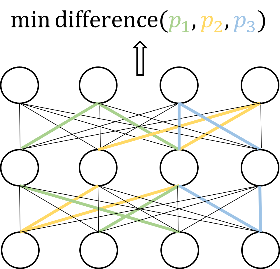
Figure 1: Illustration of the intra-distillation process. We pass the model $K$ ($K=3$) times and obtain three outputs $p_{1},p_{2},p_{3}$. Each time we disable different subsets of parameters (illustrated by different colors). Minimizing the difference of the $K$ outputs approximates minimizing the contribution difference of these disabled subsets of parameters, which can significantly improve model generalization performance.

Exploring efficient parameter use in neural networks is critical for improving computational quality and decreasing storage requirements (Han et al., 2015; Li et al., 2016). The lottery ticket hypothesis (Frankle and Carbin, 2018) suggests that a small subset of parameters, namely ‘winning tickets’, can reach similar performance compared to a dense model through iterative retraining. Recent techniques for pruning models (Lubana and Dick, 2021; Sanh et al., 2020; Xiao et al., 2019; Molchanov et al., 2016) have shown to be successful in reducing redundant parameters of trained networks by over 80% without obvious loss of the model quality. Despite the success of winning tickets, it usually does not offer better performance and is actually computationally expensive to obtain (needing iterative pruning and retraining). Moreover, unstructured pruning barely accelerates inference computation because the device still computes the dense tensors, with the only difference being that they are filled with zeros.

The main motivation behind pruning is the existence of redundant parameters which basically have no contribution to the model. Taking an opposite approach from pruning redundant parameters, we encourage all parameters to contribute. Qiao et al. (2019); Liang et al. (2022) recently showed that redundant parameters are insufficiently trained, and can actually contribute more when they are trained properly. Following this line, we also argue that there is a large room for improving model generalization by making redundant parameters contribute instead of discarding them. However, our approach differs in that we change the training objective, as opposed to learning rates.

In this paper, we show significant improvement after balancing the contribution of all parameters on various tasks. Our goal is to balance the sensitivity of parameters to encourage the equal contribution of each parameter, where sensitivity is a gradient-based measure reflecting the degree of parameter contribution. Usually, lower-sensitivity parameters are considered redundant. However, in an extreme case of our goal, no parameter is redundant. Thus, we propose intra-distillation, a task-agnostic method aiming to minimize the sensitivity difference among each subset of parameters. Specifically, we obtain $K$ outputs by forward passing the model $K$ times, where we randomly disable a different subset of parameters for each pass (Figure 1). We deduce that minimizing the difference of these $K$ outputs approximates minimizing the sensitivity of the disabled parameters. Therefore, in each step of training, we can minimize the sensitivity of $K$ random groups of parameters. We list our main contributions are summarized as follows:

• We introduce a new concept, i.e., the degree of contribution balance, describing how balanced the contribution of all parameters is. This allows us to formally define and measure how parameters can improve task performance. Moreover, we use balanced contribution of parameters to explain the successful ‘dark knowledge’ transfer in knowledge distillation (Hinton et al., 2015) between students and teachers who use the same architecture (termed self-distillation (Furlanello et al., 2018)) (Section 2).

• We propose the intra-distillation method with its adaptive strength control, which highly balances the sensitivity (contribution) of model parameters and leads to significantly better generalization performance (Section 3).

• We conduct wide-ranging experiments on machine translation, natural language understanding, and zero-shot cross-lingual transfer that show intra-distillation outperforms multiple strong baselines by a large margin, e.g., 3.54 BLEU point gains over the transformer model on average across 8 language pairs from the IWSLT’14 translation task (Section 4).

2 Why Balance the Contribution?

We investigate the contribution difference among parameters based on an important metric, parameter sensitivity, which has been widely used in pruning under the name “importance scores” (Ding et al., 2019; Molchanov et al., 2019; Lubana and Dick, 2021). Then, we highlight that model performance benefits from balanced parameter contribution in a case study of knowledge distillation.

2.1 Sensitivity Definition

The sensitivity (also named importance scores) of a set of parameters represents the impact on the loss magnitude when the parameters are zeroed-out. It suggests that higher-sensitivity parameters contribute more to the loss. Consider a model paramterized as $\bm{\Theta}$. We denote the model loss as $\mathcal{L}(\bm{\Theta})$, gradient of the loss with respect to the model parameters as $\nabla_{\bm{\Theta}}\mathcal{L}(\bm{\Theta})$, the sensitivity of a set of parameters $\bm{\Theta}_{s}$ as $\mathcal{I}(\bm{\Theta}_{s})$, model parameters with zeroed $\bm{\Theta}_{s}$ as $\bm{\Theta}_{-s}$. We evaluate sensitivity of $\bm{\Theta}_{s}$ by how much loss is preserved after zeroing $\bm{\Theta}_{s}$.

$$\mathcal{I}(\bm{\Theta}_{s})=|\mathcal{L}(\bm{\Theta})-\mathcal{L}(\bm{\Theta}_{-s})|$$ (1)

The equation above implies that the larger the absolute loss change, the more sensitive $\bm{\Theta}_{s}$ is and the more contribution to the loss it makes. However, it is not practical to forward pass the model every time to compute the sensitivity of an arbitrary set of parameters. Thus, we utilize a first-order Taylor expansion of $\mathcal{L(\cdot)}$ with respect to $\bm{\Theta}_{s}$ at $\bm{\Theta}$ to approximate $\mathcal{I}(\bm{\Theta}_{s})$.

$$\mathcal{I}(\bm{\Theta}_{s})\approx|\bm{\Theta}_{s}^{T}\nabla_{\bm{\Theta}}\mathcal{L}(\bm{\Theta})|$$ (2)

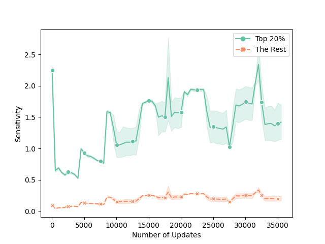
Figure 2: The mean sensitivity along with the number of training updates of top 20% most sensitive parameters and the rest of 80% parameters. Though the top 20% of parameters have significant variance in sensitivity at various stages of training, the bottom 80% consistently have very little sensitivity.

2.2 Contribution Gap Among Parameters

Previous model pruning studies (Sanh et al., 2020; Xiao et al., 2019) have shown that a small subset of parameters (e.g., 20%) are extraordinarily effective for training, and the model performance is not significantly sacrificed after pruning. We attribute the success of pruning to the much larger contribution of high-sensitivity parameters over low-sensitivity parameters. We take machine translation on the IWSLT’14 German$\rightarrow$English (De$\rightarrow$En) dataset as our study object. We focus on the transformer${}_{\texttt{small}}$ architecture (Vaswani et al., 2017). We use Equation 2 to track the sensitivity of each individual parameter and visualize the mean sensitivity of the current top 20% most sensitive parameters and the rest of 80% parameters with the increasing of training updates in Figure 2. The sensitivity of the remaining 80% of parameters are small and close to zero, but much larger for the top 20% parameters.

2.3 Benefits of Balanced Contribution

We highlight the large contribution gap between parameters, and argue that the success of pruning is due to the modest contribution of low-sensitivity parameters. However, we take an alternative argument and pose the questions: Do we overlook possible contributions of the low-sensitivity parameters when focusing on high sensitivity parameters? Will model performance improve when all parameters in a model contribute equally? Here, we first define the degree of contribution balance and investigate a case study on knowledge distillation to show the benefits of more balanced contribution.

Degree of Contribution Balance

We define the degree of contribution balance to be simply evaluating the standard deviation of all parameter sensitivity. A lower standard deviation means that there is a more balanced contribution.

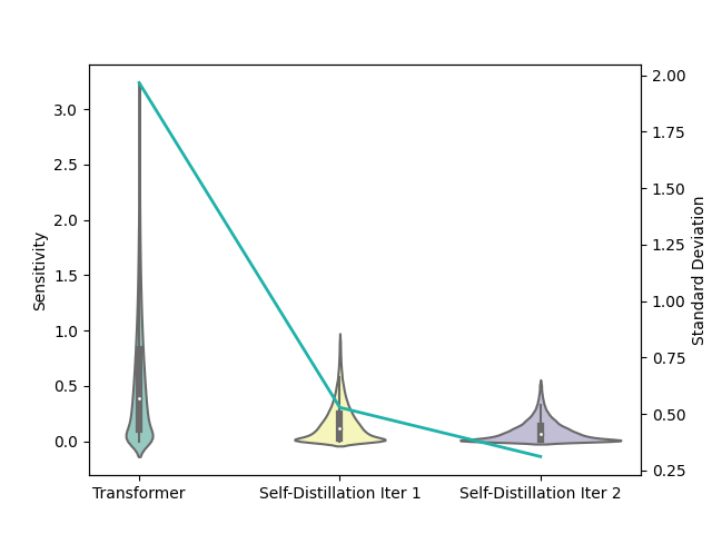
Figure 3: Sensitivity distribution (violin plots aligned with left y-axis) along with their standard deviation (green curve aligned with right y-axis) in each iteration of self-distillation (the student and teacher use the same architecture).

Method	De$\rightarrow$En
Transformer	33.07
Self-Distillation Round 1	34.87
Self-Distillation Round 2	35.03

Table 1: SacreBLEU of iterative self-distillation on IWSLT’14 De$\rightarrow$En task.

A Case Study on Knowledge Distillation

We here take naive knowledge distillation (KD) (Hinton et al., 2015) as a case study. We tie the success of KD to the more balanced contribution among parameters. KD aims to transfer knowledge from a teacher model to a student model. Specifically, the student model tries to minimize the Kullback–Leibler (KL) divergence between its output $p_{s}$ and the gold label $y$, and between $p_{s}$ and output of the teacher $p_{t}$. We here formulate a naive KD objective.

$$\min\mathbbm{KL}(y\parallel p_{s})+\mathbbm{KL}(p_{t}\parallel p_{s})$$ (3)

Commonly, the teacher is a high-capacity model and student is more compact. However, recent studies (Furlanello et al., 2018; Zhang et al., 2019; Fang et al., 2020) show that the student model can significantly outperform the teacher when the student use the same architecture (and consequently, number of parameters) as the teacher, termed self-distillation. Using the previously described machine translation task in Section 2.2, we conduct self-distillation experiments and iterate self-distillation twice, i.e., the student taught by the regular transformer model becomes a new teacher for the next student. In Table 1, we report sacreBLEU (Post, 2018). Similar to the previous literature, model performance substantially increase after each round of self-distillation. This surprising result is referred to in the literature as ’dark knowledge’ (Gotmare et al., 2018; Zhang et al., 2019). Some studies try to understand the ‘dark knowledge’, e.g., in the view of regularization (Yuan et al., 2020) or ensemble (Allen-Zhu and Li, 2020), but they only explain how it leads to performance improvements instead of how the model itself changes. Here, we argue that the ‘dark knowledge’ transferred from teachers to such students is actually due to the more balanced contribution among parameters. We visualize the sensitivity distribution of all models via violin plots with their standard deviation in Figure 3. Importantly, the parameter sensitivity becomes more balanced after each round of self-distillation. We therefore argue that the effectiveness of self-distillation is caused by more balanced parameter contribution.

Even though we hypothesize that balanced contributions explain why models improve under self-distilation, balanced contribution is not a sufficient condition for model improvement. For instance, in an extreme case, all parameter values are 0, indicating that all parameters have equal contribution, but the model performance is nonsense. However, we hypothesize that the model generalization performance benefits from the constraints of contribution balance during training. Hence, this motivates us to propose a constraint term during training to improve the model generalization performance.

3 Proposed Method

In the previous section, we showed two important findings; the large contribution gap between high- and low-sensitivity parameters, and that there is little understanding of the correlation between the better performance and more balanced contribution in self-distillation. In this section, we propose a general method to balance the parameter sensitivity (contribution) to improve the model performance.

3.1 Intra-Distillation

The sensitivity of parameters implies the degree of their contribution. We define our problem into minimizing the sensitivity difference among parameter groups. We randomly sample $K$ small groups of parameters $\{\bm{\Theta}_{s^{1}},\cdots,\bm{\Theta}_{s^{i}},\cdots,\bm{\Theta}_{s^{K}}\}$. Balancing sensitivity among all groups can be formulated as the following problem:

$$\min\sum_{i=1}^{K}\sum_{j=1}^{K}|\mathcal{I}(\bm{\Theta}_{s^{i}})-\mathcal{I}(\bm{\Theta}_{s^{j}})|.$$ (4)

Based on Equation 1, it is equivalent to

$$\min\sum_{i=1}^{K}\sum_{j=1}^{K}\bigl{|}|\mathcal{L}(\bm{\Theta})-\mathcal{L}(\bm{\Theta}_{-s^{i}})|-\\ |\mathcal{L}(\bm{\Theta})-\mathcal{L}(\bm{\Theta}_{-s^{j}})|\bigr{|}.$$ (5)

Recall that $\bm{\Theta_{-s^{i}}}$ refers to the all parameters but zeroing out $\bm{\Theta_{s^{i}}}$. To facilitate training by not calculating $\mathcal{L}(\bm{\Theta})$ , we instead minimize the upper bound of the above objective.

$$\min\sum_{i=1}^{K}\sum_{j=1}^{K}|\mathcal{L}(\bm{\Theta}_{-s^{i}})-\mathcal{L}(\bm{\Theta}_{-s^{j}})|$$ (6)

We denote the outputs of the model with $\bm{\Theta}_{-s^{i}}$ and $\bm{\Theta}_{-s^{j}}$ as $p_{i}$ and $p_{j}$, respectively. When we dissect Equation 6 deeper, it actually tries to minimize the difference between $\mathcal{D}(y,p_{i};\bm{\Theta}_{-s^{i}})$, the distance of the gold labels $y$ and $p_{i}$, and $\mathcal{D}(y,p_{j};\bm{\Theta}_{-s^{j}})$, the distance of $y$ and $p_{j}$

$$\min\sum_{i=1}^{K}\sum_{j=1}^{K}|\mathcal{D}(y,p_{i};\bm{\Theta}_{-s^{i}})-\mathcal{D}(y,p_{j};\bm{\Theta}_{-s^{j}})|,$$ (7)

where $\mathcal{D}$ can be any similarity metrics, e.g., mean squared error (MSE) for regression tasks and Kullback–Leibler (KL) divergence for classification tasks. Instead of considering the loss difference between each pair of $p_{i}$ and $p_{j}$, we straightforwardly minimize the outputs $\{p_{1},\cdots,p_{i},\cdots,p_{K}\}$ without using $y$ as an intermediary. Most deep learning tasks can be categorized into classification and regression tasks. The outputs of classification tasks are probabilities while outputs of regression tasks could be any values. For classification tasks to which most NLP problems are boiled down, we propose a novel method, X-divergence, to measure the similarity among multiple distribution based on Jensen–Shannon (JS) divergence. We finalize our loss function to balance the parameter sensitivity as follows:

$$\begin{gathered}\mathcal{L}_{id}=\frac{1}{K}\sum_{i=1}^{K}\mathbbm{KL}(p_{i}\parallel\bar{p})+\mathbbm{KL}(\bar{p}\parallel p_{i})\\ \text{where }\bar{p}=\frac{1}{K}\sum_{i=1}^{K}p_{i}.\end{gathered}$$ (8)

Here, we reduce the computation complexity from $\mathcal{O}(K^{2})$ to $\mathcal{O}(K)$ compared to Equation 7. Different from the JS divergence that only calculates the KL divergence between $p_{i}$ and the ‘center’ of all distributions $\bar{p}$, X-divergence also considers the KL divergence between $\bar{p}$ and $p_{i}$. We show that our X-divergence substantially outperforms JS divergence in Section 4.2.

For regression tasks, we simply replace X-divergence with MSE to measure their similarity.

$$\mathcal{L}_{id}=\frac{1}{K}\sum_{i=1}^{K}(p_{i}-\bar{p})^{2}$$ (9)

3.2 Task-Agnostic Implementation

Intra-Distillation is easily implemented into any deep learning task, without any model architecture modification. As presented in the previous Section 3.1, our final intra-distillation objective is to minimize the ‘distance’ of $K$ outputs generated by sub-models which have $K$ different groups of disabled parameters. In the practical implementation, we run a forward-pass of the model $K$ times. For each pass, we use dropout to simulate disabling a small subset of parameters, and obtain the output. Thus, the final loss objective we want to optimize is composed of the regular training loss from each pass $\mathcal{L}(\bm{\Theta}_{-s^{i}})$ and intra-distillation loss $\mathcal{L}_{id}$.

$$\min\frac{1}{K}\sum_{i=1}^{K}\mathcal{L}(\bm{\Theta}_{-s^{i}})+\alpha\mathcal{L}_{id}$$ (10)

$\alpha$ is a hyper-parameter to control the strength of intra-distillation. The composition of the final loss is similar to the knowledge distillation loss in Equation 3. However, our second term minimizes the difference of outputs from the same model while knowledge distillation minimizes the difference between the student and teacher (an external model).

3.3 Adaptive Intra-Distillation

We notice that the intra-distillation term could slow down the convergence speed at the beginning of training, especially when it comes to a large $\alpha$ such as 5 or 10. More details will be discussed in Section 5.2. Hence, we design an adaptive $\alpha$ algorithm that makes $\alpha$ small at the beginning of training and then becomes large afterwards to accelerate the convergence speed. Ideally, $\alpha$ grows slowly at first and gets large quickly in the middle of training. We denote $N$ as the total number of training steps and $x$ as current step. Our adaptive $\alpha^{\prime}$ is formulated as follows.

$$\alpha^{\prime}=\begin{cases}\frac{p^{\gamma}\alpha}{N^{\gamma}}x^{\gamma}&x<\frac{N}{p}\\ \alpha&x\geq\frac{N}{p}\end{cases}$$ (11)

$$\text{where }\gamma=\log_{\frac{p}{q}}\frac{1}{\alpha}$$ (12)

An illustration of the growth of $\alpha^{\prime}$ is shown in Figure 4. Here, $p$ and $q$ are two sentinels ($q$ > $p$ > 0) to control the growth speed of $\alpha^{\prime}$. Before the number of updates hits $\frac{N}{q}$, $\alpha^{\prime}$ increase slowly from 0 to 1, because we want the model to pay less attention to intra-distillation. When training achieves $\frac{N}{q}$, $\alpha^{\prime}$ is 1. $\mathcal{L}_{sd}$ now has the same weight as ordinary training loss. Then, the weight of intra-distillation should be raised substantially. $\alpha^{\prime}$ increase quickly from 1 to $\alpha$ before update step achieves $\frac{N}{p}$. At the end, $\alpha^{\prime}$ will be $\alpha$ constantly in the rest of the training steps. Note that we only apply adaptive intra-distillation in the case of $\alpha>1$. Otherwise, it is unnecessary to use adaptive learning.

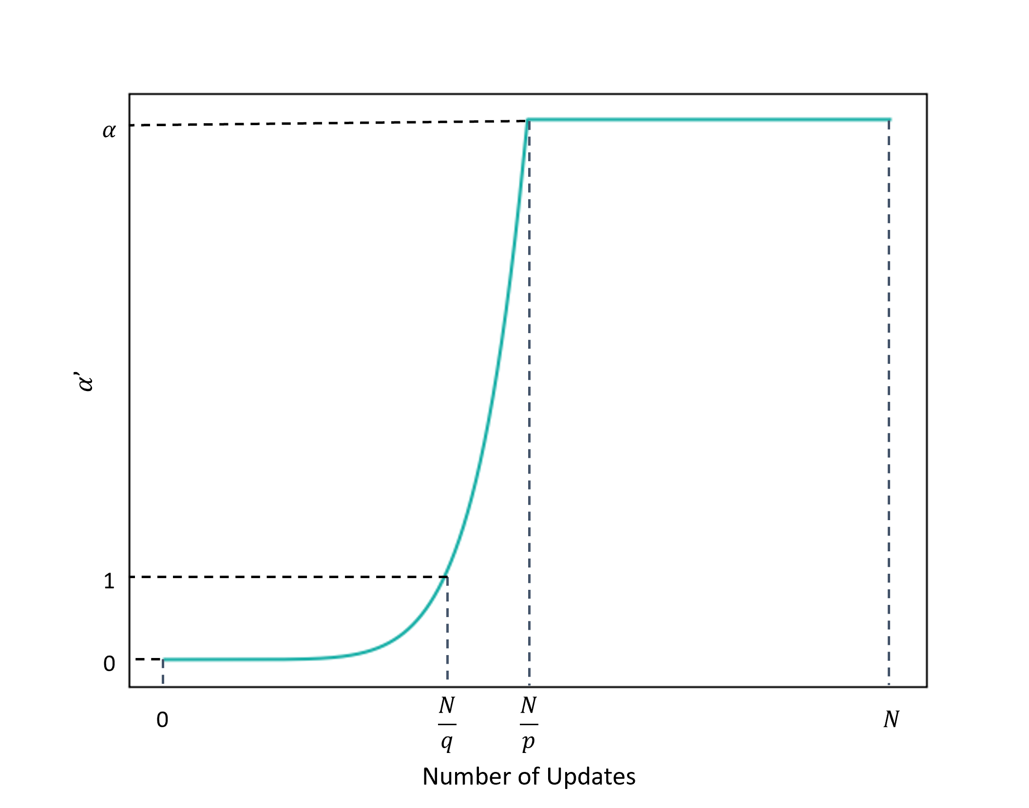
Figure 4: An example of how $\alpha^{\prime}$ increase with the control of $p$ and $q$. The relationship between $\frac{p}{q}$ and $\alpha$ determine shape (power) of the function. In a special case, adaptive learning is a linear increase if $q=\alpha p$.

$p$ and $q$ are two flexible hyper-parameters to control the weighting assigned to the intra-distillation during training. Note that a linear increase is a special case when $q=\alpha p$.

Methods	Ar	De	Es	Fa	He	It	Nl	Pl	Avg.	# parameters
Transformer (Vaswani et al., 2017)	28.62	33.07	38.89	19.64	35.13	32.76	35.90	19.69	30.46	49.98M
SAGE (Liang et al., 2022)	29.76	33.51	39.22	20.01	36.19	32.77	36.12	20.45	31.00	49.98M
R-Drop (Wu et al., 2021)	32.58	35.43	41.00	22.80	38.63	34.96	38.01	23.24	33.33	49.98M
Switch Transformer (Fedus et al., 2021)	28.24	33.11	38.43	19.50	34.42	31.93	34.59	19.82	30.00	87.81M
Intra-Distillation (JS Divergence, Ours)	32.68	35.19	41.44	22.78	38.66	34.89	38.16	23.12	33.37	49.98M
Intra-Distillation (X-Divergence, Ours)	33.42	36.10	41.82	23.78	39.31	35.43	38.53	23.61	34.00	49.98M

Table 2: Results of 8 language pairs (Xx$\rightarrow$En) on the IWSLT’14 dataset.

Methods	En$\rightarrow$De	# parameters
Transformer (Vaswani et al., 2017)	27.56	275M
SAGE (Liang et al., 2022)	27.76	275M
R-Drop (Wu et al., 2021)	28.10	275M
Switch Transformer (Fedus et al., 2021)	27.80	577M
Intra-Distillation (Ours)	28.62	275M

Table 3: Results of the WMT’17 En$\rightarrow$De task.

Methods	QNLI	MNLI-m/mm	CoLA	QQP	STS-B	RTE	SST-2	MRPC	Avg.
	Acc.	Acc.	Mcc.	F1	P/S Corr.	Acc.	Acc.	F1	Score
$\text{BERT}_{\text{base}}$ (Devlin et al., 2019)	90.6	84.7/83.6	54.0	71.1	86.6	66.8	93.4	88.6	79.93
SAGE (Liang et al., 2022)	90.8	84.9/83.8	54.5	71.3	87.1	69.8	94.1	89.7	80.67
R-Drop (Wu et al., 2021)	91.2	85.0/84.3	54.0	72.3	87.1	66.6	93.8	88.1	80.27
Intra-Distillation (Ours)	91.7	85.2/84.2	55.1	72.4	87.5	67.5	94.1	89.0	80.74

Table 4: Results of the GLUE benchmark.

4 Experiments

We evaluate our method on widely used benchmarks for machine translation, natural language understanding and zero-shot cross-lingual transfer. We pass the model $K=3$ times for all experiments. We explain the influence of $K$ in Section 5.3. Note that we briefly describe key training settings for each task but leave details in Appendix A.

4.1 Baselines

We consider three baselines in our experiments. All baseline results are from our implementation and followed by the settings from the original papers.

SAGE

SAGE (Liang et al., 2022) is a sensitivity-guided adaptive learning rate method, which encourages all parameters to be trained sufficiently by assigning higher learning rates to low-sensitivity parameters, and vice versa. SAGE is on the same study line of salience of redundant parameters as ours but using different methods.

R-Drop

R-drop (Wu et al., 2021) is a recently proposed state-of-the-art method that focuses on minimizing the inconsistency between training and inference, rather than focusing on parameter sensitivity. However though motivated differently, this method derives a similar loss objective to our proposed intra-distillation. They pass the model twice and minimize the difference of two outputs by using the Jeffrey divergence (the term for the symmetric KL). However, the advantage of X-divergence is that it is bounded while Jeffrey divergence is not, which makes training more stable. We show that our proposed X-divergence for multi-pass learning with adaptive $\alpha^{\prime}$ can achieve superior performance. Interestingly, we theoretically prove that Jeffrey divergence is the upper bound of X-divergence in Appendix C.

Switch Transformer

Scaling up the number of parameters has been usually used for improving model performance. To show the parameter efficiency of our method, We also compare our method to a well-known sparsely activated model, switch transformer (Fedus et al., 2021), in machine translation tasks. Considering the huge memory expense, we here only consider 4-expert switch transformer.

4.2 Machine Translation

Data and Settings

We consider both low- and high- resource data conditions. For the low-resource scenario, we collect 8 English-centric language pairs from IWSLT’14 (Xx$\rightarrow$En), including Arabic (Ar), German (De), Spanish (Es), Farsi (Fa), Hebrew (He), Italian (It), Dutch (Nl), Polish (Pl). The training pairs ranges from 89K to 160K. We use the transformer${}_{\texttt{small}}$ architecture (Vaswani et al., 2017). We set $\alpha=5,p=5,q=10,N=50\text{K}$ for adaptive intra-distillation. For the high-resource scenario, we consider WMT 17 En$\rightarrow$De translation task, whose corpus size is 4.5M. Following Ott et al. (2019), we separate 40K training pairs as the validation set and newstest2014 as the test set. We use the transformer${}_{\texttt{big}}$ model and set $\alpha=5,p=6.25,q=10,N=50\text{K}$. For both scenarios, the dropout rate is 0.1 for attention layers and 0.3 for FFN layers. We tokenize all sentences by sentencepiece (Kudo and Richardson, 2018). We report sacreBLEU points (Post, 2018).

Results

Results for IWSLT’14 are show in Table 2. SAGE outperforms the transformer baseline by 0.54 BLEU points on average, which matches the similar improvement in Liang et al. (2022). Interestingly, the switch transformer is not parameter-efficient when we double the parameters. At best, it only provides modest improvements in some experiments and even degenerates the performance in others. R-drop is the most competitive method. However, we still achieve the best performance by boosting the transformer model 3.54 BLEU points on average. Moreover, Our X-divergence outperform JS divergence by 0.63 on average. In Table 3, similar observations also holds for the WMT’17 task, where we achieve the highest improvement (1.06 BLEU).

4.3 Natural Language Understanding

Data and Settings

We evaluate our methods and baselines on the General Language Understanding Evaluation (GLUE) benchmark (Wang et al., 2018). We fine-tune pre-trained BERT (Devlin et al., 2019) base model on each task of GLUE. We follow the hyperparameter settings suggested by Liu et al. (2020). To have a fair comparison to SAGE, we adopt Adamax (Kingma and Ba, 2014) optimizer. The dropout rate is 0.1. $\alpha$ for each task is in the range of {0.5, 1.0, 1.5}. Recall that we do not apply adaptive $\alpha$ to intra-distillation if $\alpha\leq 1$.

Results

We report the result of GLUE test set in Table 4. Scores are calculated by GLUE online evaluation server. SAGE and our method achieve similar gains (0.74 vs. 0.79) over the BERT baseline on average. However, our method performs much better on large datasets, e.g., QNLI (105K) with a gain of 1.1, QQP (364K) with a gain of 1.3, while SAGE achieves modest improvements on these tasks. On the other hand, interestingly, SAGE is more effective on small datasets, e.g., RTE (2.4K) with a gain of 3.0 and MRPC (3.7K) with a gain of 1.1. Our method also outperform R-Drop by 0.47 on average.

Method	NER	TyDiQA
XLM-R	64.6	55.8
XLM-R + Intra-Distillation	66.0	58.0

Table 5: Zero-shot cross-lingual transfer results (F1 score) on NER and TyDiQA. The scores are averaged by all languages and 5 trials with different random seeds.

4.4 Cross-Lingual Transfer

Data and Settings

We consider a low-level and a high-level task for zero-shot cross-lingual transfer, i.e., Wikiann Named-Entity Recognition (NER) task (Pan et al., 2017) and Typologically Diverse Question Answering-Gold Passage (TyDiQA) (Artetxe et al., 2020). We download datasets from the XTREME-R benchmark (Ruder et al., 2021). NER and TyDiQA cover 48 and 9 languages, respectively. Following Xu and Murray (2022), the model architecture of NER is based on pre-trained XLM-R${}_{\text{large}}$ attached with a feed-forward token-level classifier. For TydiQA, the representations of all subwords in XLM-R${}_{\texttt{base}}$ are input to a span classification head –– a linear layer computing the start and the end of the answer. The models are only trained on English and then evaluated on all languages. We set dropout rate as 0.1 and run 10 and 15 epochs for NER and TyDiQA, both with $\alpha=1$.

Results

Averaged results (F1 scores) among all languages are shown in Table 5. We run the model 5 times with 5 different random seeds and report the averaged F1 score. The models have better overall performance after applying intra-distillation. NER achieves 1.4 F1 improvement on average. The high-lever task, TyDiQA, benefits more from intra-distillation, and obtain 2.2 F1 improvement. Please find full results on all languages in Appendix D.

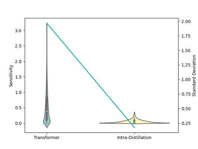
Figure 5: Sensitivity distribution comparison along with their standard deviation between the models with and without using intra-distillation on the IWSLT’14 De$\rightarrow$En MT task.

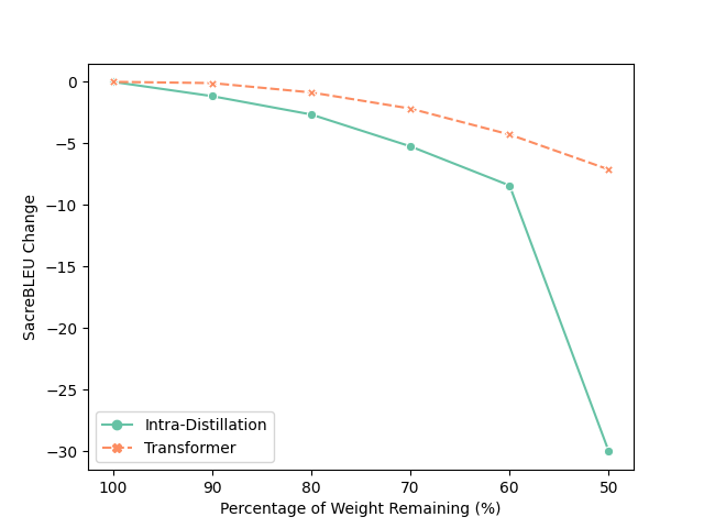
(a) Change in BLEU scores

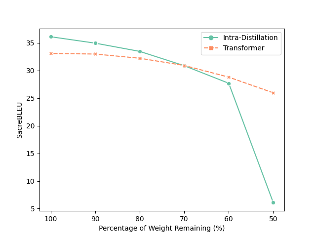
(b) BLEU scores

Figure 6: Model performance with different pruning ratio for the translation task.

5 Analysis

5.1 More Balanced Contribution

We here focus on analyzing IWSLT’14 De$\rightarrow$En translation task, but we also show the similar findings on the QQP task in Appendix E. We show the sensitivity distribution comparison with and without intra-distillation in Figure 5. The sensitivity is computed on the model which performs best on the valid set. After intra-distillation, sensitivity distribution is more concentrated, implying parameter contribution is more balanced as our goal.

We are also interested in the contribution of parameters with respect to the downstream metric. We compare a typically trained transformer model to one trained with intra-disillation, pruning up to 50% of the parameters. We prune parameters in order of sensitivity, starting with the least sensitive parameters. As shown in Figure 6, BLEU drops significantly faster for the intra-distillation model, as more parameters are pruned. This suggests that the low-sensitivity parameters of the intra-distilled model contribute much more (to task performance) than in the regular transformer model, so the model generalization degenerates faster without them. Particularly, we observe that intra-distillation significantly improves the contribution of the parameters within the lowest 40%-50% parameter range. After removing them, BLEU further drops around 20 points (yielding a BLEU score near 5, which is basically an unintelligible translation), but the regular transformer only drops less than 3 points and still scores over 25 BLEU in total. Thus, intra-distillation shows the importance of these lower-sensitivity parameters and the significant performance degeneration after pruning them.

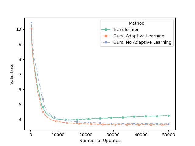
Figure 7: Valid loss curves comparison between intra-distillation with and without adaptive learning. We also add the loss curve of regular transformer as a reference.

5.2 Adaptive Learning for Intra-Distillation

We here show how the adaptive learning method helps convergence. We conduct an apples-to-apples comparison in IWSLT’14 De$\rightarrow$En translation task between intra-distillation with and without dynamic $\alpha^{\prime}$. Our $\alpha$ is 5 as set above. As shown in Figure 7, without adaptive learning, the valid loss is substantially higher than the loss of the regular transformer at the beginning of training. However, adaptive learning eliminates this issue and the loss even drops faster than the baseline model. Moreover, the valid loss with adaptive learning is always lower than the one without adaptive learning at the same training step.

5.3 Number of Model Passes

We examine the impact of the number of model passes $K$. We conduct experiments for IWSLT’14 De$\rightarrow$En with various $K$ ranging from 2 to 6. Figure 8 shows that multi-pass training is crucial to the model performance. The resultant gain obtained is 0.4 when we increase from 2 passes to 3 passes. However, the performance is similar if the number of passes is larger than 3. Although the 4-pass model works slightly better than 3-pass model, we still pass the model 3 times for all tasks considering the computational cost and slight improvement.

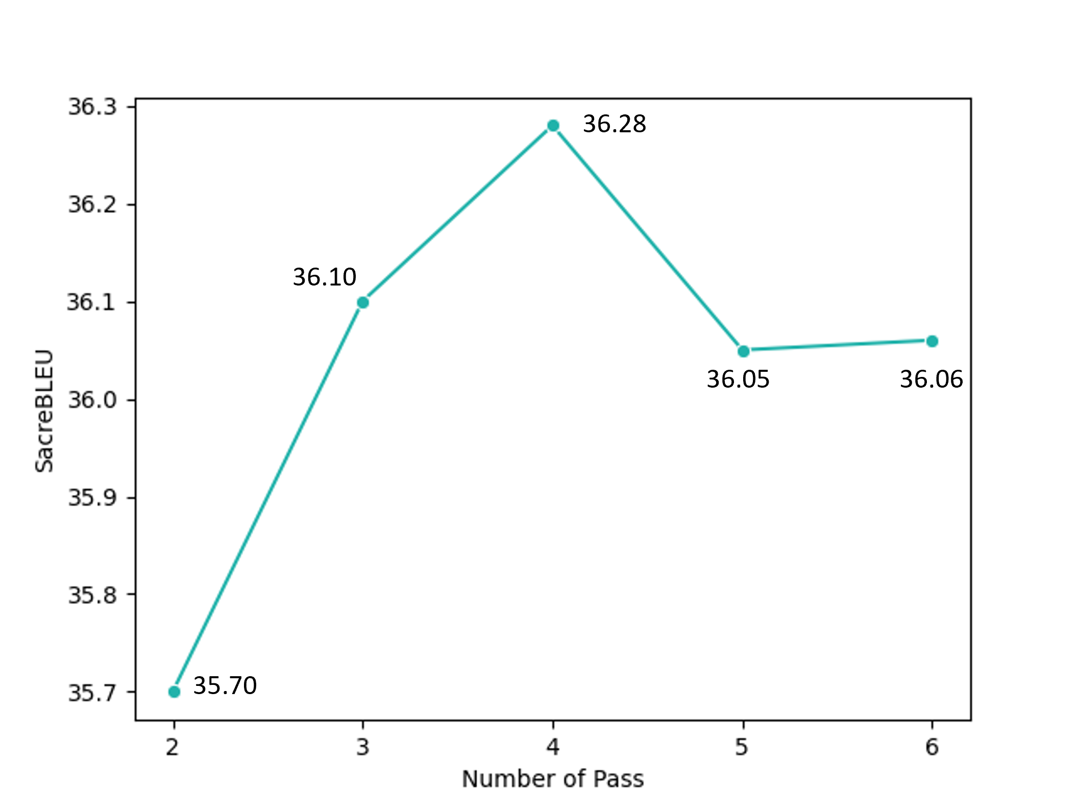
Figure 8: IWSLT’14 De$\rightarrow$En BLEU vs. number of model passes $K$.

6 Conclusions

Taking an opposite view from pruning redundant parameters, we questioned whether we overlook the potential of these redundant parameters and encouraged all parameters to contribute equally to improve the model generalization performance. We first introduced the concept of degree of contribution balance to describe how balanced of all parameters is. Then, we used balanced parameter contribution to explain the ‘dark knowledge’ that successfully transfers in knowledge distillation, by analyzing the contribution gap among parameters within a model. With the goal of adding a constraint term to balance the parameter contribution, we proposed intra-distillation with a strength-adaptive learning method. With wide-ranging experiments and analysis on machine translation, natural language understanding and zero-shot cross-lingual transfer tasks, we demonstrated that intra-distillation are capable of improving the model performance significantly and balance the parameter contribution effectively.

Limitations

This method modifies the training objective and is not specific to data. As such, any standard limitation of a neural training method will apply here, such as biases in data, hyperparameter choices, etc. However, being data agnostic also implies that the method should in theory be language and task agnostic. We’ve shown improvements on multiple languages from diverse language families on multiple tasks, yet naturally, this list is non-exhaustive and limited to the NLP domain. We expect the method generalizes to tasks outside of language, but have not explored these. Furthermore, since we need to pass the model $K$ times, the method incurs a higher time cost (or more memory cost if we concatenate the same $K$ inputs for one pass computation). However, though this cost is a limitation, we argue that it is acceptable given a user is cognizant of this and compares it to the improved performance.

Appendix A Training Details

A.1 IWSLT’14 Translation

We use the same training configuration for all 8 language pairs. We filter out the training pairs whose length ratio is larger than 1.5 or one of length is longer than 175 tokens. We use small transformer architecture (Vaswani et al., 2017), with FFN dimension size 1024, attention dimension size 512 and 4 attention heads. The batch size is 4096 tokens. We jointly train a 12K bilingual vocabulary by using sentencepiece (Kudo and Richardson, 2018) for each language pair. The maximum learning rate is 0.0005. The optimizer is Adam (Kingma and Ba, 2014) with inverse_sqrt learning rate scheduler and weight decay of 0.0001. The maximum training update is 50K with 8K warm-up steps. At inference time, we use beam search with width 5 and use a length penalty of 1.

A.2 WMT’17 Translation

We filter out the training pairs whose length ratio is larger than 1.5 or one of length is longer than 256 tokens. We use large transformer architecture (Vaswani et al., 2017), with FFN dimension size 4096, attention dimension size 1024 and 16 attention heads. The batch size is 4096 tokens but we accumulate gradients for 16 times. We jointly train a 32K bilingual vocabulary by using sentencepiece (Kudo and Richardson, 2018). The maximum learning rate is 0.0005. The optimizer is Adam (Kingma and Ba, 2014) with inverse_sqrt learning rate scheduler and weight decay of 0.0001. The maximum training update is 50K with 4K warm-up steps. At inference time, we use beam search with width 4 and use a length penalty of 0.6.

A.3 GLUE benchmark

We use pre-trained BERT${}_{\texttt{base}}$ model (Devlin et al., 2019) and fine-tune it on each GLUE task. We set the maximum sentence length as 128. Batch size is 32 sentences. The optimizer is Adamax (Kingma and Ba, 2014) with 2e-4 learning rate. We run 20 epochs for each task. The result for STS-B is the Pearson correlation. Matthew’s correlation is used for CoLA. F1 is used for QQP and MRPC. Other tasks are measured by Accuracy. We leave the detailed settings of $\alpha$, $p$ and $q$ of every GLUE task in Table 6.

	QNLI	MNLI	CoLA	QQP	STS-B	RTE	SST-2	MRPC
$\alpha$	0.5	0.5	0.5	0.5	1	1	0.5	1.5
$p$	-	-	-	-	-	-	-	6.67
$q$	-	-	-	-	-	-	-	10

Table 6: Settings of $\alpha$, $p$ and $q$ of every task at GLUE benchmark.

A.4 Xtreme-R Benchmark

We consider NER and TyDiQA tasks to evaluate the effectiveness of intra-distillation in zero-shot cross-lingual transfer learning. NER and TyDiQA respectively contains 48 and 9 languages. For NER, we use XLM-R${}_{\texttt{large}}$ model architecture (Conneau et al., 2020). The max length is 128. We train the model for 10 epochs with learning rate 2e-5, batch size 8 and gradient accumulation 4. For TyDiQA, we use XLM-R${}_{\texttt{base}}$ model architecture. The max length is 384. We train the model for 15 epochs with learning rate 3e-5, batch size 8 and gradient accumulation 4.

Appendix B Sensitivity Distribution Visualization Details

Sensitivity of each parameter approximates to the absolute multiplication of its value and gradient. We randomly pick 100 batches and feed to the model to retrieve the gradients. Note that We also remove the top 1% highest-sensitive parameters to ease the illustration. We store the sensitivity of each parameter and randomly sample 10% of them to visualize them via violin plots.

Appendix C The Bound of X-Divergence

Here, we show that our X-divergence is upper bounded by the Jeffrey divergence. Usually, Jeffrey divergence only serves for two distributions:

$$J(p_{1},p_{2})=\mathbbm{KL}(p_{1}\parallel p_{2})+\mathbbm{KL}(p_{2}\parallel p_{1})$$ (13)

We generalize it to measure multiple (say, $K$) distributions:

$$J(p_{1},\cdots,p_{K})=\sum_{i=1}^{K}\sum_{j=1}^{K}\mathbbm{KL}(p_{i}\parallel p_{j})\\ +\mathbbm{KL}(p_{j}\parallel p_{i})$$ (14)

Our proposed X-divergence is formulated as follows:

$$X(p_{1},\cdots,p_{K})=\frac{1}{K}\sum_{i=1}^{K}\mathbbm{KL}(p_{i}\parallel\bar{p})\\ +\mathbbm{KL}(\bar{p}\parallel p_{i})$$ (15)

Theorem C.1.

X-divergence is upper bounded by the Jeffrey Divergence:

$$X(p_{1},\cdots,p_{K})\leq\frac{1}{K^{2}}J(p_{1},\cdots,p_{K})$$ (16)

Proof.

We separate the proof in two parts. We prove that the first and second term of $J$ divergence are the upper bound of the first and second term of X-divergence, respectively, i.e.,

$$\frac{1}{K}\sum_{i=1}^{K}\mathbbm{KL}(p_{i}\parallel\bar{p})\leq\frac{1}{K^{2}}\sum_{i=1}^{K}\sum_{j=1}^{K}\mathbbm{KL}(p_{i}\parallel p_{j})$$ (17)

and

$$\frac{1}{K}\sum_{i=1}^{K}\mathbbm{KL}(\bar{p}\parallel p_{i})\leq\frac{1}{K^{2}}\sum_{i=1}^{K}\sum_{j=1}^{K}\mathbbm{KL}(p_{j}\parallel p_{i}).$$ (18)

We first prove the Equation 17. Since each $p_{i}\geq 0$, by the inequality of the arithmetic and geometric means, we have

$$\frac{\sum_{i=1}^{K}p_{i}}{K}\geq\sqrt[K]{\prod_{i=1}^{K}p_{i}}.\$$

Thus, it follows

$$\begin{split}&\frac{1}{K}\sum_{i=1}^{K}\mathbbm{KL}(p_{i}\parallel\bar{p})\\ &=\frac{1}{K}\sum_{i=1}^{K}p_{i}\log(\frac{p_{i}}{\frac{\sum_{j=1}^{K}p_{j}}{K}})\\ &\leq\frac{1}{K}\sum_{i=1}^{K}p_{i}\log(\frac{p_{i}}{\sqrt[K]{\prod_{j=1}^{K}p_{j}}})\\ &=\frac{1}{K}\sum_{i=1}^{K}p_{i}(\log p_{i}-\frac{\sum_{j=1}^{K}\log p_{j}}{K})\\ &=\frac{1}{K}\sum_{i=1}^{K}p_{i}\frac{\sum_{j=1}^{K}\log p_{i}-\log p_{j}}{K}\\ &=\frac{1}{K^{2}}\sum_{i=1}^{K}\sum_{j=1}^{K}p_{i}log\frac{p_{i}}{p_{j}}\\ &=\frac{1}{K^{2}}\sum_{i=1}^{K}\sum_{j=1}^{K}\mathbbm{KL}(p_{i}\parallel p_{j}).\end{split}$$

Now, we have proved the Equation 17, and move to the proof of Equation 18. Consider that the function $f(x)=x\log x$ is a convex function. Based on the Jensen’s inequality, we have

$$\frac{\sum_{i=1}^{K}p_{i}}{K}\log(\frac{\sum_{i=1}^{K}p_{i}}{K})\leq\frac{1}{K}(\sum_{i=1}^{K}p_{i}\log p_{i}).$$

Thus, it follows

$$\begin{split}&\frac{1}{K}\sum_{i=1}^{K}\mathbbm{KL}(\bar{p}\parallel p_{i})\\ &=\frac{1}{K}\sum_{i=1}^{K}\frac{\sum_{j=1}^{K}p_{j}}{K}(\log\frac{\sum_{j=1}^{K}p_{j}}{K}-\log p_{i})\\ &\leq\frac{1}{K}\sum_{i=1}^{K}\frac{\sum_{j=1}^{K}p_{j}\log p_{j}}{K}-\frac{\sum_{j=1}^{K}p_{j}\log p_{i}}{K}\\ &=\frac{1}{K^{2}}\sum_{i=1}^{K}\sum_{j=1}^{K}p_{j}\log\frac{p_{j}}{p_{i}}\\ &=\frac{1}{K^{2}}\sum_{i=1}^{K}\sum_{j=1}^{K}\mathbbm{KL}(p_{j}\parallel p_{i}).\end{split}$$

We also have proved the Equation 18. Thus, the proof of Equation 16 is done.

∎

Appendix D Full Results of Zero-Shot Cross-Lingual Transfer

We leave the full results of zero-shot cross-lingual transfer learning on the NER, TyDiQA task in Table 7 and Table 8, respectively.

Methods	ar	he	vi	id	jv	ms	tl	eu	ml	ta	te	af	nl	en	de	el	bn	hi	mr	ur	fa	fr	it	pt	es
XLM-R	45.75	55.35	78.67	52.47	61.35	69.65	71.95	56.37	65.79	55.82	52.85	78.34	83.76	84.50	78.78	78.38	74.39	69.71	61.87	54.85	56.82	79.78	81.39	81.91	76.64
XLM-R + Intra-Distillation	49.26	53.31	77.65	53.15	63.89	71.13	75.70	62.91	62.97	59.66	51.53	79.30	84.39	85.40	78.59	80.97	76.82	71.54	63.46	56.05	51.28	80.68	81.78	82.46	76.61
	bg	ru	ja	ka	ko	th	sw	yo	my	zh	kk	tr	et	fi	hu	qu	pl	uk	az	lt	pa	gu	ro	Avg.
XLM-R	81.32	70.60	18.31	66.37	57.28	1.02	69.86	32.90	51.97	27.06	50.46	79.30	77.79	79.65	80.13	54.62	80.89	74.48	67.61	76.87	48.62	61.59	82.98	64.56
XLM-R + Intra-Distillation	82.46	70.87	21.67	67.46	56.04	1.76	70.09	39.77	57.62	29.19	53.84	78.48	78.65	80.87	81.33	56.93	82.38	80.65	70.47	78.90	51.43	64.49	90.90	65.97

Table 7: Full results (F1) of the zero-shot cross-lingual NER task.

Methods	ar	bn	fi	id	ko	ru	sw	te	en	Avg.
XLM-R	62.53	42.24	61.82	70.62	42.99	57.75	56.40	43.23	65.51	55.80
XLM-R + Intra-Distillation	67.03	41.24	62.54	74.91	44.50	59.46	57.07	47.29	68.20	58.03

Table 8: Full results (F1) of the zero-shot cross-lingual TyDiQA task.

Appendix E More Balanced Contribution in The QQP Task

Similar to the findings in Section 5.1, sensitivity of all parameters becomes more balanced after using intra-distillation (Figure 9). Moreover, in the one-shot unstructured pruning, performance of the model which is trained with intra-distillation drops faster than the regular model (Figure 10). This also implies that lower-sensitivity parameters contribute more than the regular ones.

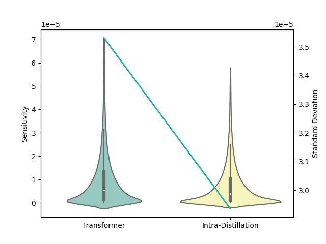
Figure 9: Sensitivity distribution comparison along with their standard deviation between the models with and without using intra-distillation on the QQP task.

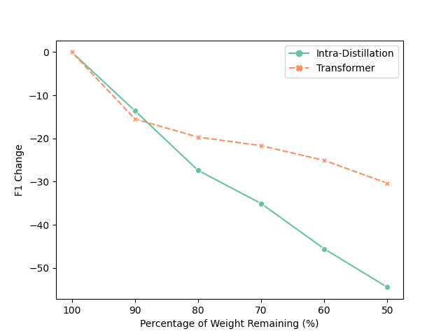
(a) Change in F1 scores

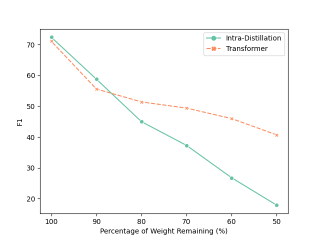
(b) F1 scores

Figure 10: Model performance with different pruning ratio for the QQP task.

References

- Allen-Zhu and Li (2020) Zeyuan Allen-Zhu and Yuanzhi Li. 2020. Towards understanding ensemble, knowledge distillation and self-distillation in deep learning. arXiv preprint arXiv:2012.09816.
- Artetxe et al. (2020) Mikel Artetxe, Sebastian Ruder, and Dani Yogatama. 2020. On the Cross-lingual Transferability of Monolingual Representations. In Proceedings of ACL 2020.
- Conneau et al. (2020) Alexis Conneau, Kartikay Khandelwal, Naman Goyal, Vishrav Chaudhary, Guillaume Wenzek, Francisco Guzmán, Édouard Grave, Myle Ott, Luke Zettlemoyer, and Veselin Stoyanov. 2020. Unsupervised cross-lingual representation learning at scale. In Proceedings of the 58th Annual Meeting of the Association for Computational Linguistics, pages 8440–8451.
- Devlin et al. (2019) Jacob Devlin, Ming-Wei Chang, Kenton Lee, and Kristina Toutanova. 2019. Bert: Pre-training of deep bidirectional transformers for language understanding. In Proceedings of the 2019 Conference of the North American Chapter of the Association for Computational Linguistics: Human Language Technologies, Volume 1 (Long and Short Papers), pages 4171–4186.
- Ding et al. (2019) Xiaohan Ding, Xiangxin Zhou, Yuchen Guo, Jungong Han, Ji Liu, et al. 2019. Global sparse momentum sgd for pruning very deep neural networks. Advances in Neural Information Processing Systems, 32.
- Fang et al. (2020) Zhiyuan Fang, Jianfeng Wang, Lijuan Wang, Lei Zhang, Yezhou Yang, and Zicheng Liu. 2020. Seed: Self-supervised distillation for visual representation. In International Conference on Learning Representations.
- Fedus et al. (2021) William Fedus, Barret Zoph, and Noam Shazeer. 2021. Switch transformers: Scaling to trillion parameter models with simple and efficient sparsity. arXiv preprint arXiv:2101.03961.
- Frankle and Carbin (2018) Jonathan Frankle and Michael Carbin. 2018. The lottery ticket hypothesis: Finding sparse, trainable neural networks. In International Conference on Learning Representations.
- Furlanello et al. (2018) Tommaso Furlanello, Zachary Lipton, Michael Tschannen, Laurent Itti, and Anima Anandkumar. 2018. Born again neural networks. In International Conference on Machine Learning, pages 1607–1616. PMLR.
- Gotmare et al. (2018) Akhilesh Gotmare, Nitish Shirish Keskar, Caiming Xiong, and Richard Socher. 2018. A closer look at deep learning heuristics: Learning rate restarts, warmup and distillation. In International Conference on Learning Representations.
- Han et al. (2015) Song Han, Jeff Pool, John Tran, and William Dally. 2015. Learning both weights and connections for efficient neural network. Advances in neural information processing systems, 28.
- Hinton et al. (2015) Geoffrey Hinton, Oriol Vinyals, Jeff Dean, et al. 2015. Distilling the knowledge in a neural network. arXiv preprint arXiv:1503.02531, 2(7).
- Kingma and Ba (2014) Diederik P Kingma and Jimmy Ba. 2014. Adam: A method for stochastic optimization. arXiv preprint arXiv:1412.6980.
- Kudo and Richardson (2018) Taku Kudo and John Richardson. 2018. SentencePiece: A simple and language independent subword tokenizer and detokenizer for neural text processing. In Proceedings of the 2018 Conference on Empirical Methods in Natural Language Processing: System Demonstrations, pages 66–71, Brussels, Belgium. Association for Computational Linguistics.
- Li et al. (2016) Hao Li, Asim Kadav, Igor Durdanovic, Hanan Samet, and Hans Peter Graf. 2016. Pruning filters for efficient convnets. arXiv preprint arXiv:1608.08710.
- Liang et al. (2022) Chen Liang, Haoming Jiang, Simiao Zuo, Pengcheng He, Xiaodong Liu, Jianfeng Gao, Weizhu Chen, and Tuo Zhao. 2022. No parameters left behind: Sensitivity guided adaptive learning rate for training large transformer models. In International Conference on Learning Representations.
- Liu et al. (2020) Xiaodong Liu, Yu Wang, Jianshu Ji, Hao Cheng, Xueyun Zhu, Emmanuel Awa, Pengcheng He, Weizhu Chen, Hoifung Poon, Guihong Cao, et al. 2020. The microsoft toolkit of multi-task deep neural networks for natural language understanding. In Proceedings of the 58th Annual Meeting of the Association for Computational Linguistics: System Demonstrations, pages 118–126.
- Lubana and Dick (2021) Ekdeep Singh Lubana and Robert Dick. 2021. A gradient flow framework for analyzing network pruning. In International Conference on Learning Representations.
- Molchanov et al. (2019) Pavlo Molchanov, Arun Mallya, Stephen Tyree, Iuri Frosio, and Jan Kautz. 2019. Importance estimation for neural network pruning. In Proceedings of the IEEE/CVF Conference on Computer Vision and Pattern Recognition, pages 11264–11272.
- Molchanov et al. (2016) Pavlo Molchanov, Stephen Tyree, Tero Karras, Timo Aila, and Jan Kautz. 2016. Pruning convolutional neural networks for resource efficient inference. arXiv preprint arXiv:1611.06440.
- Ott et al. (2019) Myle Ott, Sergey Edunov, Alexei Baevski, Angela Fan, Sam Gross, Nathan Ng, David Grangier, and Michael Auli. 2019. fairseq: A fast, extensible toolkit for sequence modeling. In Proceedings of the 2019 Conference of the North American Chapter of the Association for Computational Linguistics (Demonstrations), pages 48–53, Minneapolis, Minnesota. Association for Computational Linguistics.
- Pan et al. (2017) Xiaoman Pan, Boliang Zhang, Jonathan May, Joel Nothman, Kevin Knight, and Heng Ji. 2017. Cross-lingual name tagging and linking for 282 languages. In Proceedings of ACL 2017, pages 1946–1958.
- Post (2018) Matt Post. 2018. A call for clarity in reporting BLEU scores. In Proceedings of the Third Conference on Machine Translation: Research Papers, pages 186–191, Brussels, Belgium. Association for Computational Linguistics.
- Qiao et al. (2019) Siyuan Qiao, Zhe Lin, Jianming Zhang, and Alan L. Yuille. 2019. Neural rejuvenation: Improving deep network training by enhancing computational resource utilization. In Proceedings of the IEEE/CVF Conference on Computer Vision and Pattern Recognition (CVPR).
- Ruder et al. (2021) Sebastian Ruder, Noah Constant, Jan Botha, Aditya Siddhant, Orhan Firat, Jinlan Fu, Pengfei Liu, Junjie Hu, Dan Garrette, Graham Neubig, and Melvin Johnson. 2021. XTREME-R: Towards more challenging and nuanced multilingual evaluation. In Proceedings of the 2021 Conference on Empirical Methods in Natural Language Processing, pages 10215–10245, Online and Punta Cana, Dominican Republic. Association for Computational Linguistics.
- Sanh et al. (2020) Victor Sanh, Thomas Wolf, and Alexander Rush. 2020. Movement pruning: Adaptive sparsity by fine-tuning. Advances in Neural Information Processing Systems, 33:20378–20389.
- Vaswani et al. (2017) Ashish Vaswani, Noam Shazeer, Niki Parmar, Jakob Uszkoreit, Llion Jones, Aidan N Gomez, Łukasz Kaiser, and Illia Polosukhin. 2017. Attention is all you need. Advances in neural information processing systems, 30.
- Wang et al. (2018) Alex Wang, Amanpreet Singh, Julian Michael, Felix Hill, Omer Levy, and Samuel R Bowman. 2018. Glue: A multi-task benchmark and analysis platform for natural language understanding. In International Conference on Learning Representations.
- Wu et al. (2021) Lijun Wu, Juntao Li, Yue Wang, Qi Meng, Tao Qin, Wei Chen, Min Zhang, Tie-Yan Liu, et al. 2021. R-drop: regularized dropout for neural networks. Advances in Neural Information Processing Systems, 34.
- Xiao et al. (2019) Xia Xiao, Zigeng Wang, and Sanguthevar Rajasekaran. 2019. Autoprune: Automatic network pruning by regularizing auxiliary parameters. Advances in neural information processing systems, 32.
- Xu and Murray (2022) Haoran Xu and Kenton Murray. 2022. Por qué não utiliser alla språk? mixed training with gradient optimization in few-shot cross-lingual transfer. In Findings of the Association for Computational Linguistics: NAACL 2022, pages 2043–2059, Seattle, United States. Association for Computational Linguistics.
- Yuan et al. (2020) Li Yuan, Francis EH Tay, Guilin Li, Tao Wang, and Jiashi Feng. 2020. Revisiting knowledge distillation via label smoothing regularization. In Proceedings of the IEEE/CVF Conference on Computer Vision and Pattern Recognition, pages 3903–3911.
- Zhang et al. (2019) Linfeng Zhang, Jiebo Song, Anni Gao, Jingwei Chen, Chenglong Bao, and Kaisheng Ma. 2019. Be your own teacher: Improve the performance of convolutional neural networks via self distillation. In Proceedings of the IEEE/CVF International Conference on Computer Vision, pages 3713–3722.