Instance-Based Uncertainty Estimation for Gradient-Boosted Regression Trees

Abstract

Gradient-boosted regression trees (GBRTs) are hugely popular for solving tabular regression problems, but provide no estimate of uncertainty. We propose Instance-Based Uncertainty estimation for Gradient-boosted regression trees (IBUG), a simple method for extending any GBRT point predictor to produce probabilistic predictions. IBUG computes a non-parametric distribution around a prediction using the $k$-nearest training instances, where distance is measured with a tree-ensemble kernel. The runtime of IBUG depends on the number of training examples at each leaf in the ensemble, and can be improved by sampling trees or training instances. Empirically, we find that IBUG achieves similar or better performance than the previous state-of-the-art across 22 benchmark regression datasets. We also find that IBUG can achieve improved probabilistic performance by using different base GBRT models, and can more flexibly model the posterior distribution of a prediction than competing methods. We also find that previous methods suffer from poor probabilistic calibration on some datasets, which can be mitigated using a scalar factor tuned on the validation data. Source code is available at https://github.com/jjbrophy47/ibug.

1 Introduction

Despite the impressive success of deep learning models on unstructured data (e.g., images, audio, text), gradient-boosted trees [26] remain the preferred choice for tabular or structured data [52]. In fact, Kaggle CEO Anthony Goldbloom recently described gradient-boosted trees as the most “glaring difference” between what is used on Kaggle and what is “fashionable in academia” [34].

Our focus is on tabular data for regression tasks, which vary widely from financial [1] and retail-product forecasting [43] to weather [29, 28] and clinic-mortality prediction [6]. Gradient-boosted regression trees (GBRTs) are known to make accurate point predictions [42] but provide no estimate of the prediction uncertainty, which is desirable for both forecasting practitioners [9, 68] and the explainable AI (XAI) community [25, 69, 2] in general. Recently,  Duan et al. [22], Sprangers et al. [64], and Malinin et al. [44] introduced NGBoost, PGBM, and CBU (CatBoost [52] with uncertainty), respectively, new gradient boosting algorithms that provide state-of-the-art probabilistic predictions. However, NGBoost tends to underperform as a point-predictor, and PGBM and CBU are limited in the types of distributions they can use to model the output.

We introduce a simple yet effective method for enabling any GBRT point-prediction model to produce probabilistic predictions. Our proposed approach, Instance-Based Uncertainty estimation for Gradient-boosted regression trees (IBUG), has two key components: 1) We leverage the fact that GBRTs accurately model the conditional mean and use this point prediction as the mean in a probabilistic forecast; and 2) We identify the $k$ training examples with the greatest affinity to the target instance and use these examples to estimate the uncertainty of the target prediction. We define the affinity between two instances as the number of times both instances appear in the same leaf throughout the ensemble. Thus, our method acts as a wrapper around any given GBRT model.

In experiments on 21 regression benchmark datasets and one synthetic dataset, we demonstrate the effectiveness of IBUG to deliver on par or improved probabilistic performance as compared to existing state-of-the-art methods while maintaining state-of-the-art point-prediction performance. We also show that probabilistic predictions can be improved by applying IBUG to different GBRT models, something that NGBoost and PGBM cannot do. Additionally, IBUG can use the training instances closest to the target example to directly model the output distribution using any parametric or non-parametric distribution, something NGBoost, PGBM, and CBU cannot do. Finally, we show that sampling trees dramatically improves runtime efficiency for computing training-example affinities without having a significant detrimental impact on the resulting probabilistic predictions, allowing IBUG to scale to larger datasets.

2 Notation & Background

We assume an instance space $\mathcal{X}\subseteq\mathbb{R}^{p}$ and target space $\mathcal{Y}\subset\mathbb{R}$. Let $\mathcal{D}\coloneqq\{(x_{i},y_{i})\}_{i=1}^{n}$ be a training dataset in which each instance $x_{i}\in\mathcal{X}$ is a $p$-dimensional vector $(x_{i}^{j})_{j=1}^{p}$ and $y_{i}\in\mathcal{Y}$.

2.1 Gradient-Boosted Regression Trees

Gradient-boosting [26] is a powerful machine-learning algorithm that iteratively adds weak learners to construct a model $f:\mathcal{X}\rightarrow\mathbb{R}$ that minimizes some empirical risk $\mathcal{L}:\mathbb{R}\times\mathbb{R}\rightarrow\mathbb{R}$. The model is defined by a recursive relationship: $f_{0}(x)=\gamma$, $\dots$, $f_{t}(x)=f_{t-1}(x)+\eta\ m_{t}(x)$ in which $f_{0}$ is the base learner, $\gamma$ is an initial estimate, $f_{t}$ is the model at iteration $t$, $m_{t}$ is the weak learner added during iteration $t$ to improve the model, and $\eta$ is the learning rate.

Gradient-boosted regression trees (GBRTs) typically choose $\ell$ to be the mean squared error (MSE), $\gamma$ as $\frac{1}{n}\sum_{i=1}^{n}y_{i}$ (mean output of the training instances), and regression trees as weak learners. Each weak learner is typically chosen to approximate the negative gradient [44]: $m_{t}=\operatorname*{arg\,min}_{m}\ \frac{1}{n}\sum_{i=1}^{n}(-g_{t}^{i}-m(x_{i}))^{2}$ in which $g_{t}^{i}=\frac{\partial\ell(y_{i},\hat{y}_{i})}{\partial\hat{y}_{i}}$ is the functional gradient of the $i$th training instance at iteration $t$ with respect to $\hat{y}_{i}=f_{t-1}(x_{i})$.

The weak learner at iteration $t$ recursively partitions the instance space into $M_{t}$ disjoint regions $\{{r_{t}^{j}}\}_{j=1}^{M_{t}}$. Each region is called a leaf, and the parameter value for leaf $j$ at tree $t$ is typically determined (given a fixed structure) using a one-step Newton-estimation method [36]: $\theta_{t}^{j}=-\sum_{i\in I_{t}^{j}}g_{t}^{i}/(\sum_{i\in I_{t}^{j}}h_{t}^{i}+\lambda$) in which $I_{t}^{j}=\{{(x_{i},y_{i})\mid x_{i}\in r_{t}^{j}}\}_{i=1}^{n}$ is the instance set of leaf $j$ for tree $t$, $h_{t}^{i}$ is the second derivative of the $i$th training instance w.r.t. $\hat{y}_{i}$, and $\lambda$ is a regularization constant. Thus, the output of $m_{t}$ can be written as follows: $m_{t}(x)=\sum_{j=1}^{M_{t}}\theta_{t}^{j}\ \mathbbm{1}[x\in r_{t}^{j}]$ in which $\mathbbm{1}$ is the indicator function. The final GBRT model generates a prediction for a target example $x_{te}$ by summing the values of the leaves $x_{te}$ traverses to across all $T$ iterations: $\hat{y}_{te}=\sum_{t=1}^{T}m_{t}(x_{te})$.

2.2 Probabilistic Regression

Our focus is on probabilistic regression—estimating the conditional probability distribution $P(y|x)$ for some target variable $y$ given some input vector $x\in\mathcal{X}$. Unfortunately, traditional GBRT models only output scalar values. Under a squared-error loss function, these scalar values can be interpreted as the conditional mean in a Gaussian distribution with some (unknown) constant variance. However, homoscedasticity is a strong assumption and unknown constant variance has little value in a probabilistic prediction; thus, in order to allow heteroscedasticity, the predicted distribution needs at least two parameters to convey both the magnitude and uncertainty of the prediction [22].

Natural Gradient Boosting (NGBoost) is a recent method by Duan et al. [22] that tackles the aforementioned problems by estimating the parameters of a desired distribution using a multi-parameter boosting approach that trains a separate ensemble for each parameter of the distribution. NGBoost employs the natural gradient to be invariant to parameterization, but requires the inversion of many small matrices (each the size of the number of parameters) to do so. Empirically, NGBoost generates state-of-the-art probabilistic predictions, but tends to underperform as a point predictor.

More recently, Sprangers et al. [64] introduced Probabilistic Gradient Boosting Machines (PGBM), a single model that optimizes for point performance, but can also generate accurate probabilistic predictions. PGBM treats leaf values as stochastic random variables, using sample statistics to model the mean and variance of each leaf value. PGBM estimates the output mean and variance of a target example using the estimated parameters of each leaf it is assigned to. The predicted mean and variance are then used as parameters in a specified distribution to generate a probabilistic prediction. PGBM has been shown to produce state-of-the-art probabilistic predictions; however, computing the necessary leaf statistics during training can be computationally expensive, especially as the number of leaves in the ensemble increases (see §5.6). Also, since only the mean and variance are predicted for a given target example, PGBM is limited to distributions using only location and scale to model the output.

Finally, Malinin et al. [44] introduce CatBoost with uncertainty (CBU), a method that estimates uncertainty using ensembles of GBRT models. Similar to NGBoost, multiple ensembles are learned to output the mean and variance. However, CBU also constructs a virtual ensemble—a set of overlapping partitions of the learned GBRT trees—to estimate the uncertainty of a prediction by taking the mean of the variances output from the virtual ensemble. Their approach uses a recently proposed stochastic gradient Langevin boosting algorithm [72] to sample from the true posterior via the virtual ensmble (in the limit); however, their formulation of uncertainty is limited only to the first and second moments, similar to PGBM.

To address the shortcomings of existing approaches, we introduce a simple method that performs well on both point and probabilistic performance, and can more flexibly model the output than previous approaches. Our method can also be applied to any GBRT model, adding additional flexibility.

3 Instance-Based Uncertainty

Instance-based methods such as $k$-nearest neighbors have been around for decades and have been useful for many different machine learning tasks [50]. However, defining neighbors based on a fixed metric like Euclidean distance may lead to suboptimal performance, especially as the dimensionality of the dataset increases. More recently, it has been shown that random forests can be used as an adaptive nearest neighbors method [18, 40] which identifies the most similar examples to a given instance using the learned model structure. This supervised tree kernel can more effectively measure the similarity between examples, and has been used for clustering [46] and local linear modeling [8] as well as instance-[11] and feature-based attribution explanations [51], for example.

In this work, we apply the idea of a supervised tree kernel to help model the uncertainty of a given GBRT prediction. Our approach, Instance-Based Uncertainty estimation for Gradient-boosted regression trees (IBUG), identifies the neighborhood of similar training examples to a target example using the structure of the GBRT, and then uses those instances to generate a probabilistic prediction. IBUG works for any GBRT, and can more flexibly model the output than competing methods.

3.1 Identification of High-Affinity Neighbors

At its core, IBUG uses the $k$ training examples with the largest affinity to the target example to model the conditional output distribution. Given a GBRT model $f$, we define the affinity between two examples simply as the number of times each instance appears in the same leaf across all trees in $f$. Thus, the affinity of the $i$th training example $x_{i}$ to a target example $x_{te}$ can be written as:

$$A(x_{i},x_{te})=\sum_{i=1}^{T}\mathbbm{1}[R_{t}(x_{i})=R_{t}(x_{te})],$$ (1)

in which $R_{t}(x_{i})$ is the leaf $x_{i}$ is assigned to for tree $t$. Alg. 1 summarizes the procedure for computing affinity scores for all training examples. This metric clusters similar examples together based on the learned model representation (i.e., the tree structures). Intuitively, if two examples appear in the same leaf in every tree throughout the ensemble, then both examples are predicted in an identical manner. One may also view Eq. (1) as an indication of which training examples most often affect the leaf values $x_{te}$ is assigned to and thus implicitly which examples are likely to have a big effect on the prediction $\hat{y}_{te}$. This similarity metric is similar to the random forest kernel [18], however, unlike random forests, GBRTs are typically constructed to a shallower depth, resulting in more training examples assigned to the same leaf (see §C.5 for additional details about leaf density in GBRTs).

Algorithm 1 IBUG affinity computation.

1:Input instance $x\in\mathcal{X}$, GBRT model $f$.

2:procedure ComputeAffinities($x$, $f$)

3:    $A\leftarrow\vec{0}$ $\triangleright$ Init. train affinities

4:    for $t=1\ldots T$ do $\triangleright$ Visit each tree

5:        Get instance set $I_{t}^{l}$ for leaf $l=R_{t}(x)$

6:        for $i\in I_{t}^{l}$ do $\triangleright$ Increment affinities

7:           $A_{i}\leftarrow A_{i}+1$             

8:return $A$

Algorithm 2 IBUG probabilistic prediction.

1:Input $x\in\mathcal{X}$, GBRT model $f$, $k$ highest-affinity neighbors $A^{(k)}$, min. variance $\rho$, variance calibration parameters $\gamma$ and $\delta$, target distribution $D$.

2:procedure ProbPredict($x$, $f$, $A^{(k)}$, $\rho$, $\gamma$, $\delta$, $D$)

3:    $\mu_{\hat{y}}\leftarrow f(x)$ $\triangleright$ GBRT scalar output

4:    $\sigma^{2}_{\hat{y}}\leftarrow\max(\sigma^{2}($$A^{(k)}$$),\ \rho)$ $\triangleright$ Ensure $\sigma^{2}>0$

5:    $\sigma^{2}_{\hat{y}}\leftarrow\gamma\sigma^{2}_{\hat{y}}+\delta$ $\triangleright$ Var. calibration, Eq. (2)

6:return $D(A^{(k)}|\mu_{\hat{y}},\sigma^{2}_{\hat{y}})$ $\triangleright$ Eq. (3)

3.2 Modeling the Output Distribution

IBUG has a multitude of choices when modeling the conditional output distribution. The simplest and most common approach is to model the output assuming a Gaussian distribution [22, 64]. We use the scalar output of $f$: $\mu_{\hat{y}_{te}}=f(x_{te})$ to model the conditional mean since GBRTs already produce accurate point predictions. Then, we use the $k$ training instances with the largest affinity to $x_{te}$—we denote this set $A^{(k)}$—to compute the variance $\sigma^{2}_{\hat{y}_{te}}$.

Calibrating prediction variance.

The $k$-nearest neighbors generally do a good job of determining the relative uncertainty of different predictions, but on some datasets, the resulting variance is systematically too large or too small. To correct for this, we apply an additional affine transformation before making the prediction:

$$\sigma^{2}_{\hat{y}_{te}}\leftarrow\gamma\sigma^{2}_{\hat{y}_{te}}+\delta,$$ (2)

where $\gamma$ and $\delta$ are tuned on validation data after $k$ has been selected. Instead of exhaustively searching over all values of $\gamma$ or $\delta$, we use either the multiplicative factor (tuning $\gamma$ with $\delta=0$) or the additive factor (tuning $\delta$ with $\gamma=1$), and choose between them using their performance on validation data.

We find this simple calibration step consistently improves probabilistic performance for not only IBUG, but competing methods as well, and at a relatively small cost compared to training the model.

Flexible posterior modeling.

In general, we can generate a probabilistic prediction using $\mu_{\hat{y}_{te}}$ and $\sigma^{2}_{\hat{y}_{te}}$ for any distribution that uses location and scale (note PGBM and CBU can only model these types of distributions). However, IBUG can additionally use $A^{(k)}$ to directly fit any continuous distribution $D$, including those with high-order moments:

$$\hat{D}_{te}=D(A^{(k)}|\mu_{\hat{y}_{te}},\sigma^{2}_{\hat{y}_{te}}).$$ (3)

Eq. (3) is defined such that $D$ can be fit directly with $A^{(k)}$ using MLE (maximum likelihood estimation) [47], or may be fit using $\mu_{\hat{y}_{te}}$ or $\sigma^{2}_{\hat{y}_{te}}$ as fixed parameter values with $A^{(k)}$ fitting any other parameters of the distribution. Overall, directly fitting all or some additional parameters in $D$—for example, the shape parameter in a Weibull distribution—is a benefit over PGBM and CBU, which can only optimize for a global shape value using a gridsearch-like approach with extra validation data.

Note that NGBoost can model any parameterized distribution, but must specify this choice before training; in contrast, IBUG can optimize this choice after training. Additionally, IBUG may choose $D$ to be a non-parametric density estimator such as KDE (kernel density estimation) [62], which PGBM, CBU, and NGBoost cannot do.

3.3 Summary

In summary, Alg. 2 provides pseudocode for generating a probabilistic prediction with IBUG. Note Algs. 1 and 2 work for any GBRT model, allowing practitioners to employ IBUG to adapt multiple different point predictors into probabilistic estimators and select the model with the best performance. Empirically, we show using different base models for IBUG can result in improved probabilistic performance than using just one (§5.3).

IBUG is a nearest neighbors approach and thus seems well-suited to estimating aleatoric uncertainty—remaining uncertainty due to irreducible error or the inherent stochasticity in the system [33]—since it can quantify the range of outcomes to be expected given the observed features. However, we use predictions on held-out data to tune the number of nearest neighbors and the variance calibration hyperparameters; thus, we effectively optimize prediction uncertainty encompassing both aleatoric uncertainty and epistemic uncertainty—error due to the imperfections of the model and the training data [20, 44]. The evaluation measures in our experiments thus also focus on predictive uncertainty.

4 Computational Efficiency

Training efficiency.

Since IBUG works with standard GBRT models, it inherits the training efficiency of modern GBRT implementations such as XGBoost [12], LightGBM [36], and CatBoost [52].

Prediction efficiency.

If there are $T$ trees in the ensemble and each leaf has at most $n_{l}$ training instances assigned to it, then IBUG’s prediction time is $O(Tn_{l})$, since it considers each instance in each leaf. Note training instances that do not appear in a leaf with the target instance do not increase prediction time; what matters most is thus the number of instances at each leaf. We find LightGBM often induces regression trees with large leaves—in some cases, over half the dataset is assigned to a single leaf (see §C.5 for details). Thus, prediction time still grows with the size of the dataset, as is typical for instance-based methods. This higher prediction time is the price IBUG pays for greater flexibility.

Prediction efficiency can be increased at training time by using deeper GBRTs with fewer instances in each leaf, after training by subsampling the instances considered for predictions, or at prediction time by sampling the trees used to compute affinities. We explore this last option in the next subsection.

4.1 Sampling Trees

The most expensive operation when generating a probabilistic prediction with IBUG is computing the affinity vector (Eq. 1). In order to increase prediction efficiency, we can instead work with a subset of the trees $\tau<T$ in the ensemble. We can build this subset by sampling trees uniformly at random, taking the first trees learned (representing the largest gradient steps), or the last trees learned (representing the fine-tuning steps).

By sampling trees, the runtime complexity reduces to $O(\tau n_{l})$, which provides significant speedups when $\tau\ll T$. In our empirical evaluation, we find that taking a subset of the first trees learned generally works best, significantly increasing prediction efficiency while maintaining accurate probabilistic predictions (§5.6).

4.2 Accelerated $k$ Tuning

Choosing an appropriate value of $k$ is critical for generating accurate probabilistic predictions in IBUG. Thus, we aim to tune $k$ using a held-out validation dataset $\mathcal{D}_{val}\subset\mathcal{D}$ and an appropriate probabilistic scoring metric such as negative log likelihood (NLL). Unfortunately, typical tuning procedures would result in the same affinity vectors being computed—an expensive operation—for each candidate value of $k$. To mitigate this issue, we perform a custom tuning procedure that reuses computed affinity vectors for all values of $k$. More specifically, IBUG computes an affinity vector $A$ for a given validation example $x_{val}$, and then sorts $A$ in descending order (i.e., largest affinity first). Then, IBUG takes the top $k$ training instances, and generates and scores the resulting probabilistic prediction. For each subsequent value of $k$, the same sorted affinity list can be used, avoiding duplicate computation. We summarize this procedure in Alg. 3.

Once $k$ is chosen, we may encounter a new unseen target instance in which the variance of the $k$-highest affinity training examples for that target example is zero or extremely small. In this case, we set the predicted target variance to $\rho$, which is set during tuning to the minimum (nonzero) variance computed over all predictions in the validation set for the chosen $k$. In practice, we find instances of abnormally low variance to be rare with appropriately chosen values of $k$.

Algorithm 3 IBUG accelerated tuning of $k$.

1:Validation dataset $\mathcal{D}_{val}\subset\mathcal{D}$, GBRT model $f$, list of candidates $K$, target distribution $D$, probabilistic scoring metric $V$, minimum variance $\rho=1\mathrm{e}{-15}$.

2:procedure FastTuneK($\mathcal{D}_{val}$, $f$, $K$, $D$, $V$, $\rho$)

3:     for $(x_{j},y_{j})\in\mathcal{D}_{val}$ do

4:         $A\leftarrow$ ComputeAffinities($x_{j},f$) $\triangleright$ Algorithm 1

5:         $A\leftarrow$ Argsort $A$ in descending order

6:         for $k\in K$ do $\triangleright$ Use same ordering for each $k$

7:              $A^{(k)}\leftarrow$ Take first $k$ training instances($A,k$)

8:              $\hat{D}_{y_{j}}^{k}\leftarrow$ ProbPredict($x_{j},f,A^{(k)},\rho,1,0,D$) $\triangleright$ Algorithm 2

9:              $S_{j}^{k}\leftarrow V(y_{j},\hat{D}_{y_{j}}^{k})$ $\triangleright$ Save validation score               

10:     $k\leftarrow$ Select best $k$ from $S$

11:     $\rho\leftarrow$ Select minimum $\sigma^{2}$ from $\hat{D}^{k}$

12:return $k$, $\rho$

5 Experiments

In this section, we demonstrate IBUG’s ability to produce competitive probabilistic and point predictions as compared to current state-of-the-art methods on a large set of regression datasets (§5.1, §5.2). Then, we show that IBUG can use different base models to improve probabilistic performance (§5.3), flexibly model the posterior distribution (§5.4), and use approximations to speed up probabilistic predictions while maintaining competitive performance (§5.6).

Implementation and Reproducibility.

We implement IBUG in Python, using Cython—a Python package allowing the development of C extensions—to store a unified representation of the model structure. IBUG supports all modern gradient boosting frameworks including XGBoost [12], LightGBM [36], and CatBoost [52]. Experiments are run on publicly available datasets using an Intel(R) Xeon(R) CPU E5-2690 v4 @ 2.6GHz with 60GB of RAM @ 2.4GHz. Links to all data sources as well as the code for IBUG and all experiments is available at https://github.com/jjbrophy47/ibug.

5.1 Methodology

We now compare IBUG’s probabilistic and point predictions to NGBoost [22], PGBM [64], and CBU [44] on 21 benchmark regression datasets and one synthetic dataset. Additional dataset details are in §B.1.

Metrics.

We compute the average continuous ranked probability score (CRPS $\downarrow$) and negative log likelihood (NLL $\downarrow$) [29, 76] over the test set to evaluate probabilistic performance. To evaluate point performance, we use root mean squared error (RMSE $\downarrow$). For all metrics, lower is better. See §B for detailed descriptions.

Protocol.

We follow a similar protocol to Sprangers et al. [64] and Duan et al. [22]. We use 10-fold cross-validation to create 10 90/10 train/test folds for each dataset. For each fold, the 90% training set is randomly split into an 80/20 train/validation set to tune any hyperparameters. Once the hyperparameters are tuned, the model is retrained using the entire 90% training set. For probabilistic predictions, a normal distribution is used to model the output.

Significance Testing.

We report counts of the number of datasets in which a given method performed better (“Win”), worse (“Loss”), or not statistically different (“Tie”) relative to a comparator using a two-sided paired t-test over the 10 random folds with a significance level of 0.05.

Hyperparameters.

We tune NGBoost the same way as in Duan et al. [22]. Since PGBM, CBU, and IBUG optimize a point prediction metric, we tune their hyperparameters similarly. We also tune variance calibration parameters $\gamma$ and $\delta$ for each method (§3.2). Exact hyperparameter values evaluated and selected are in §B.2. Unless specified otherwise, we use CatBoost [52] as the base model for IBUG.

Table 1: Probabilistic (CRPS) performance for each method on each dataset. Lower is better. Normal distributions are used for all probabilistic predictions. Results are averaged over 10 folds, and standard errors are shown in subscripted parentheses. The best method for each dataset is bolded, as well as those with standard errors that overlap the best method. Bottom row: Head-to-head comparison between IBUG/IBUG+CBU and each method showing the number of wins, ties, and losses (W-T-L) across all datasets. On average, IBUG+CBU provides the most accurate probabilistic predictions.

Dataset	NGBoost	PGBM	CBU	IBUG	IBUG+CBU
Ames	38346(547)	10872(355)	11008(330)	10434(367)	10194(368)
Bike	12.4(0.955)	1.183(0.041)	0.833(0.036)	0.974(0.048)	0.766(0.032)
California	1e11(1e11)	0.222(0.001)	0.217(0.001)	0.213(0.001)	0.207(0.001)
Communities	0.068(0.002)	0.068(0.002)	0.067(0.002)	0.065(0.002)	0.065(0.002)
Concrete	3.410(0.182)	1.927(0.086)	1.788(0.077)	1.849(0.098)	1.741(0.082)
Energy	0.519(0.043)	0.147(0.006)	0.196(0.009)	0.143(0.009)	0.157(0.008)
Facebook	4.022(0.099)	3.554(0.095)	3.211(0.059)	3.073(0.066)	2.977(0.070)
Kin8nm	0.095(0.001)	0.061(0.001)	0.057(0.001)	0.051(0.001)	0.051(0.001)
Life	2.897(1.465)	0.815(0.027)	0.772(0.024)	0.794(0.023)	0.731(0.022)
MEPS	5.527(0.196)	6.448(0.092)	6.050(0.109)	6.150(0.114)	6.016(0.113)
MSD	4.524(0.005)	4.576(0.005)	4.363(0.004)	4.410(0.005)	4.347(0.004)
Naval	0.003(0.000)	0.000(0.000)	0.000(0.000)	0.000(0.000)	0.000(0.000)
News	2191(47.5)	2361(52.6)	2346(52.6)	2545(41.0)	2380(52.1)
Obesity	3.208(0.028)	1.860(0.022)	1.740(0.017)	1.866(0.021)	1.771(0.019)
Power	2.105(0.023)	1.531(0.019)	1.473(0.022)	1.542(0.020)	1.471(0.021)
Protein	5427(5409)	1.823(0.011)	1.788(0.009)	1.784(0.008)	1.742(0.009)
STAR	132(1.589)	131(1.380)	130(1.283)	130(1.214)	129(1.198)
Superconductor	2.405(0.028)	0.126(0.004)	0.150(0.004)	0.153(0.006)	0.128(0.004)
Synthetic	5.779(0.042)	5.737(0.039)	5.739(0.040)	5.731(0.040)	5.730(0.040)
Wave	571020(883)	3891(73.9)	2349(10.3)	2679(16.0)	2026(9.538)
Wine	0.385(0.005)	0.323(0.005)	0.337(0.006)	0.322(0.006)	0.321(0.006)
Yacht	1.177(0.158)	0.292(0.042)	0.281(0.048)	0.276(0.048)	0.255(0.046)
IBUG W-T-L	17-3-2	11-9-2	9-5-8	-	1-6-15
IBUG+CBU W-T-L	17-3-2	15-6-1	18-2-2	15-6-1	-

5.2 Probabilistic and Point Performance

We first compare IBUG’s probabilistic and point predictions to each baseline on each dataset. See Table 1 for detailed CRPS results; due to space constraints, results for additional probabilistic metrics (e.g., NLL) as well as point performance results are in §B.3. Our main findings are as follows:

• On probabilistic performance, IBUG performs equally well or better than NGBoost and PGBM, winning on 17 and 11 (out of 22) datasets respectively, while losing on only 2 and 2 (respectively). Since CBU and IBUG performance is similar, we combine the two approaches, averaging their outputs; we denote this simple ensemble IBUG+CBU. Surprisingly, IBUG+CBU works very well, losing on only a maximum of 2 datasets when faced head-to-head against any other method; these results suggest IBUG and CBU are complimentary approaches.

• On point performance, PGBM, CBU, and IBUG performed significantly better than NGBoost; this is consistent with previous work and is perhaps unsurprising since NGBoost is optimized for probabilistic performance, not point performance. However, IBUG generally performed better than PGBM, winning on 13 datasets and losing on only 1 dataset; and performed slightly better than CBU, winning on 6 datasets with no losses.

We also compare IBUG with two additional baselines—$k$NN and BART [13]—shown in §C.2–C.3 due to space constraints. We find IBUG generally outperforms these methods in both probabilistic and point performance. Overall, the results in this section suggest IBUG generates both competitive probabilistic and point predictions compared to existing methods.

5.3 Different Base Models

Table 2: Probabilistic (CRPS, NLL) performance on the test set for IBUG using different base models. Results are averaged over 10 folds, and standard errors are shown in subscripted parentheses; lower is better. On 6 and 5 datasets, respectively, either IBUG-LightGBM or IBUG-XGBoost significantly outperforms IBUG-CatBoost on the validation set and subsequently on the test set, demonstrating the potential for improved probabilistic performance by using IBUG with different base models.

	Test CRPS ($\downarrow$)
Dataset	CatBoost	LightGBM	XGBoost
Bike	0.974(0.048)	0.819(0.024)	0.849(0.012)
MSD	4.410(0.005)	4.372(0.005)	4.418(0.005)
News	2545(41.0)	2436(50.8)	2551(56.0)
Power	1.542(0.020)	1.536(0.022)	1.518(0.018)
Protein	1.784(0.008)	1.683(0.009)	1.788(0.008)
Supercon.	0.153(0.006)	0.090(0.005)	0.010(0.003)

	Test NLL ($\downarrow$)
Dataset	CatBoost	LightGBM	XGBoost
Bike	1.886(0.056)	1.292(0.048)	1.662(0.024)
MSD	3.415(0.002)	3.409(0.002)	3.402(0.002)
Naval	-6.208(0.010)	-6.281(0.007)	-5.853(0.014)
Obesity	2.646(0.009)	2.593(0.016)	2.624(0.010)
Supercon.	0.783(0.181)	-0.496(0.169)	20.4(23.2)

Here we experiment using different base models for IBUG besides CatBoost [52]; specifically, we use LightGBM [36] and XGBoost [12], two popular gradient boosting frameworks. Table 2 shows that using a different base model can result in improved probabilistic performance. This highlights IBUG’s agnosticism to GBRT type, enabling practitioners to apply IBUG to future models with improved point prediction performance.

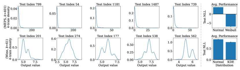
Figure 1: Left: Distribution of the $k$-nearest training examples for 5 randomly-selected test instances from the MEPS (top) and Wine (bottom) datasets. Right: Test NLL (with standard error) when modeling the posterior using two different distributions (lower is better). IBUG can model parametric and non-parametric distributions that better fit the underlying data than assuming normality.

5.4 Posterior Modeling

One of the unique benefits of IBUG is the ability to directly model the output using empirical samples (Figure 1), giving practitioners a better sense of the output distribution for specific predictions. IBUG can optimize a distribution after training, and has more flexibility in the types of distributions it can model—from distributions using just location and scale to those with high-order moments as well as non-parametric density estimators. To test this flexibility, we model each probabilistic prediction using the following distributions: normal, skewnormal, lognormal, Laplace, student t, logistic, Gumbel, Weibull, and KDE; we then select the distribution with the best average NLL on the validation set, and evaluate its probabilistic performance on the test set.

Figure 1 demonstrates that the selected distributions for the MEPS and Wine datasets achieve better probabilistic performance than assuming normality. Qualitatively, the empirical densities of $A^{(k)}$ for a randomly sampled set of test instances reaffirms the selected distributions. As an additional comparison, we report CBU achieves a test NLL of $3.699_{\pm 0.038}$ and $1.025_{\pm 0.028}$ for the MEPS and wine datasets (respectively) using a normal distribution, while IBUG achieves $-6.887_{\pm 0.260}$ and $0.785_{\pm 0.025}$ using Weibull and KDE estimation (respectively). For the MEPS dataset, the selected Weibull distribution takes a shape parameter, which IBUG estimates directly on a per prediction basis using $A^{(k)}$and MLE. In contrast, PGBM or CBU would need to optimize a global shape value using a validation set, which is likely to be suboptimal for individual predictions.

5.5 Variance Calibration

Table 3 shows probabilistic performance comparisons of each method against itself with and without variance calibration. In all cases, variance calibration (§3.2) either maintains or improves performance for all methods, especially CBU. Overall, these results suggest that variance calibration should be a standard procedure for probabilistic prediction, unless using a method that has particularly well-calibrated predictions to begin with. We therefore use variance calibration in all of our results.

Additionally, §C.1 shows performance results for all methods without variance calibration. Overall, we observe similar relative performance trends as when applying calibration (Table 1).

Table 3: Probabilistic performance comparison of each method with vs. without variance calibration. In all cases, calibration maintains or improves performance; it is especially helpful for CBU.

	CRPS			NLL
Method	Wins	ties	Losses	Wins	Ties	Losses
NGBoost	9	13	0	1	21	0
PGBM	13	9	0	11	11	0
CBU	17	5	0	11	11	0
IBUG	13	9	0	5	17	0

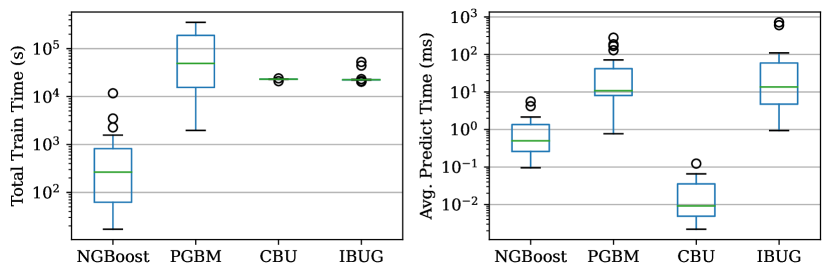
Figure 2: Runtime comparison. Left: Total train time (including tuning). Right: Average prediction time per test example. Results are shown for all datasets, averaged over 10 folds (exact values are in §B.4, Tables 12 and 13). On average, IBUG has comparable training times to PGBM and CBU, but is relatively slow for prediction.

Figure 3: Change in probabilistic (NLL) performance (top) and average prediction time (in seconds) per test example (bottom) as a function of $\tau$ for six datasets with trees sampled first-to-last; lower is better. NGBoost, PGBM, and CBU are added for additional context. The shaded regions represent the standard error. Overall, average prediction time decreases significantly as $\tau$ decreases while test NLL often remains relatively stable, enabling IBUG to generate probabilistic predictions with significant increased efficiency.

5.6 Sampling Trees

Figure 2 shows the runtime for each method broken down into total training time (including tuning) and prediction time per test example. On average, IBUG has similar training times to PGBM and CBU, but on some datasets, IBUG is roughly an order of magnitude faster than PGBM. For predictions, IBUG is similar to PGBM but relatively slow compared to NGBoost and CBU.

However, by sampling $\tau<T$ trees when computing the affinity vector, IBUG can significantly reduce prediction time. Figure 3 shows results when sampling trees first-to-last, which typically works best over all tree-sampling strategies (alternate sampling strategies are evaluated in §C.4). As $\tau$ decreases, we observe average prediction time decreases roughly 1-2 orders of magnitude while probabilistic performance remains relatively stable until $\tau/T$ reaches roughly 1–5%, at which point probabilistic performance sometimes starts to decrease more rapidly. Note for the Ames and Life datasets, IBUG can reach the same average prediction time as NGBoost while maintaining the same or better probabilistic performance than NGBoost, PGBM, and CBU. These results demonstrate that if speed is a concern, IBUG can approximate the affinity computation to speed up prediction times while maintaining competitive probabilistic performance.

6 Additonal Related Work

Traditional approaches to probabilistic regression include generalized additive models for location, scale, and shape (GAMLSS), which allow for a flexible choice of distribution for the target variable but are restricted to pre-specified model forms [56]. Prophet [68] also produces probabilistic estimates for generalized additive models, but has been shown to underperform as compared to more recent approaches [60, 3]. Bayesian methods [48, 30] naturally generate uncertainty estimates by integrating over the posterior; however, exact solutions are limited to simple models, and more complex models such as Bayesian Additive Regression Trees (BART) [13, 41] require computationally expensive sampling techniques (e.g., MCMC [4]) to provide approximate solutions.

Other approaches to probabilistic regression tasks include conformal predictions [61, 67, 5] which produce confidence intervals via empirical errors obtained in the past, and quantile regression [32, 37, 45, 57]. Similar to PGBM, distributional forests (DFs) [59] estimate distributional parameters in each leaf, and average these estimates over all trees in the forest. Deep learning approaches for probabilistic regression [54, 74, 3] have increased recently, with notable approaches such as DeepAR [58] and methods based on transformer architectures [38, 39].

7 Conclusion

IBUG uses ideas from instance-based learning to enable probabilistic predictions for any GBRT point predictor. IBUG generates probabilistic predictions by using the $k$-nearest training instances to the test instance found using the structure of the trees in the ensemble. Our results on 22 regression datasets demonstrate this simple wrapper produces competitive probabilistic and point predictions to current state-of-the-art methods, most notably NGBoost [22], PGBM [64], and CBU [44]. We also show that IBUG can more flexibly model the posterior distribution of a prediction using any parametric or non-parametric density estimator. IBUG’s one limitation is relatively slow prediction time. However, we show that approximations in the search for the $k$-nearest training instances can significantly speed up prediction time; predictions are also easily parallelizable in IBUG. For future work, we plan to investigate other approximations to the affinity vector such as subsampling or even reweighting training instances, which may lead to significant speed ups of IBUG.

Checklist

1. For all authors…

   1. Do the main claims made in the abstract and introduction accurately reflect the paper’s contributions and scope? [Yes]

   2. Did you describe the limitations of your work? [Yes] See §7.

   3. Did you discuss any potential negative societal impacts of your work? [Yes] See §A.1.

   4. Have you read the ethics review guidelines and ensured that your paper conforms to them? [Yes]

2. If you are including theoretical results…

   1. Did you state the full set of assumptions of all theoretical results? [N/A]

   2. Did you include complete proofs of all theoretical results? [N/A]

3. If you ran experiments…

   1. Did you include the code, data, and instructions needed to reproduce the main experimental results (either in the supplemental material or as a URL)? [Yes] See §5.

   2. Did you specify all the training details (e.g., data splits, hyperparameters, how they were chosen)? [Yes] See §5.1.

   3. Did you report error bars (e.g., with respect to the random seed after running experiments multiple times)? [Yes]

   4. Did you include the total amount of compute and the type of resources used (e.g., type of GPUs, internal cluster, or cloud provider)? [Yes] See §5.

4. If you are using existing assets (e.g., code, data, models) or curating/releasing new assets…

   1. If your work uses existing assets, did you cite the creators? [Yes] See §B.1.

   2. Did you mention the license of the assets? [No] The license of each asset can be found by following its corresponding citation.

   3. Did you include any new assets either in the supplemental material or as a URL? [Yes] See §5.

   4. Did you discuss whether and how consent was obtained from people whose data you’re using/curating? [N/A]

   5. Did you discuss whether the data you are using/curating contains personally identifiable information or offensive content? [N/A]

5. If you used crowdsourcing or conducted research with human subjects…

   1. Did you include the full text of instructions given to participants and screenshots, if applicable? [N/A]

   2. Did you describe any potential participant risks, with links to Institutional Review Board (IRB) approvals, if applicable? [N/A]

   3. Did you include the estimated hourly wage paid to participants and the total amount spent on participant compensation? [N/A]

Appendix A Algorithmic Details

Figure 4 summarizes how IBUG generates a probabilistic prediction for a given input instance.

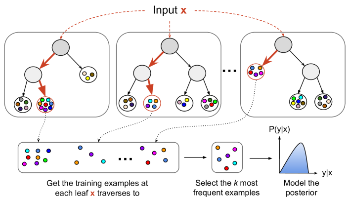
Figure 4: IBUG workflow. Given a GBRT model and an input instance $x$, IBUG collects the training examples at each leaf $x$ traverses to, keeps the $k$ most frequent examples, and then uses those examples to model the output distribution.

A.1 Ethical Statement

In general, this work has no foreseeable negative societal impacts; however, users should carefully validate their models as imprecise uncertainty estimates may adversely affect certain domains (e.g., healthcare, weather).

Appendix B Implementation and Experiment Details

We implement IBUG in Python, using Cython—a Python package allowing the development of C extensions—to store a unified representation of the model structure. IBUG currently supports all major modern gradient boosting frameworks including XGBoost [12], LightGBM [36], and CatBoost [52]. Experiments are run on an Intel(R) Xeon(R) CPU E5-2690 v4 @ 2.6GHz with 60GB of RAM @ 2.4GHz. We run our experiments on publicly available datasets. Links to all data sources as well as the code for IBUG and all experiments is currently available online at https://github.com/jjbrophy47/ibug.

Metrics.

We use the continuous ranked probability score (CRPS) and negative log likelihood (NLL) to measure probabilistic performance. CRPS is a quadratic measure of discrepancy between the cumulative distribution function (CDF) $F$ of forecast $\hat{y}$ and the empirical CDF of the scalar observation $y$: $\int(F(\hat{y})-\mathbbm{1}[\hat{y}\geq y])^{2}d\hat{y}$ in which $\mathbbm{1}$ is the indicator function [29, 76]. To evaluate point performance, we use root mean squared error (RMSE): $\sqrt{\frac{1}{n}\sum_{i=1}^{n}(y_{i}-\hat{y}_{i})^{2}}$.

B.1 Datasets

This section gives a detailed description for each dataset we use in our experiments.

• Ames [19] consists of 2,930 instances of housing prices in the Ames, Iowa area characterized by 80 attributes. The aim is to predict the sale price of a given house.

• Bike [23, 21] contains 17,379 measurements of the number of bikes rented per hour characterized by 16 attributes. The aim is to predict the number of bikes rented for a given hour.

• California [49] consists of 20,640 instances of median housing prices in various California districts characterized by 8 attributes. The aim is to predict the median housing price for the given district.

• Communities [55, 21] consists of 1,994 measurements of violent crime statistics based on crime, survey, and census data. The dataset is characterized by 100 attributes, and the aim is to predict the violent crime rate for a given population.

• Concrete [75, 21] consists of 1,030 instances of concrete characterized by 8 attributes. The aim is to predict the compressive strength of the concrete.

• Energy [70, 21] consists of 768 buildings in which each building is one of 12 different shapes and is characterized by 8 features. The aim is to predict the cooling load associated with the building.

• Facebook [63, 21] consists of 40,949 Facebook posts characterized by 53 attributes. The aim is to predict the number of comments for a given post.

• Kin8nm [73] consists of 8,192 instances of the forward kinematics of an 8 link robotic arm. The aim is to predict the forward kinematics of the robotic arm.

• Life [53] consists of 2,928 instances of life expectancy estimates for various countries during one year. Each instance is characterized by 20 attributes, and the aim is to predict the life expectancy of the country during a specific year.

• MEPS [15] consists of 16,656 instances of medical expenditure survey data. Each instance is characterized by 139 attributes, and the aim is to predict the insurance utilization for the given medical expenditure.

• MSD [7] consists of 515,345 songs characterized by 90 audio features constructed from each song. The aim is to predict what year the song was released based on the audio features.

• Naval [16, 21] consists of 11,934 instances extracted from a high-performing gas turbine simulation. Each instance is characterized by 16 features. The aim is to predict the gas turbine decay coefficient.

• News [21, 24] consists of 39,644 Mashable articles characterized by 60 features. The aim is to predict the number of shares for a given article.

• Obesity [66] contains 48,346 instances of obesity rates for different states and regions with differing socioeconomic backgrounds. Each instance is characterized by 32 attributes. The aim is to predict the obesity rate of the region.

• Power [21, 35, 71] contains 9,568 readings of a Combined Cycle Power Plant (CCPP) at full work load. Each reading is characterized by 4 features. The aim is to predict the net hourly electrical energy output.

• Protein [21] contains 45,730 tertiary-protein-structure instances characterized by 9 attributes. The aim is to predict the armstrong coefficient of the protein structure.

• STAR [21, 65] contains 2,161 student-teacher achievement scores characterized by 39 attributes. The aim is to predict the student-teacher achievement based on the given intervention.

• Superconductor [21, 31] contains 21,263 potential superconductors characterized by 81 attributes. The aim is to predict the critical temperature of the given superconductor.

• Synthetic [10, 27] is a non-linear synthetic regression dataset in which the inputs are independent and uniformly distributed on the interval $[0,1]$; the dataset contains 10,000 instances characterized by 100 attributes.

• Wave [21] consists of 287,999 positions and absorbed power outputs of wave energy converters (WECs) in four real wave scenarios off the southern coast of Australia (Sydney, Adelaide, Perth and Tasmania). The aim is to predict the total power output of a given WEC.

• Wine [17, 21] consists of 6,497 instances of Portuguese “Vinho Verde” red and white wine characterized by 11 features. The aim is to predict the quality of the wine from 0-10.

• Yacht [21] consists of 308 instances of yacht-sailing performance characterized by 6 attributes. The aim is to predict the residual resistance per unit weight of displacement.

For each dataset, we generate one-hot encodings for any categorical variable and leave all numeric and binary variables as is. Table 4 shows a summary of the datasets after preprocessing.

Table 4: Dataset summary after preprocessing.

Dataset	Source	$n$	$p$
Ames	[19]	2,930	358
Bike	[23, 21]	17,379	37
California	[49]	20,640	100
Communities	[21, 55]	1,994	100
Concrete	[75, 21]	1,030	8
Energy	[70, 21]	768	16
Facebook	[63, 21]	40,949	133
Kin8nm	[73]	8,192	8
Life	[53]	2,928	204
MEPS	[15]	15,656	139
MSD	[7]	515,345	90
Naval	[21, 16]	11,934	17
News	[21, 24]	39,644	58
Obesity	[66]	48,346	100
Power	[21, 35, 71]	9,568	4
Protein	[21]	45,730	9
STAR	[21, 65]	2,161	95
Superconductor	[21, 31]	21,263	82
Synthetic	[10, 27]	10,000	100
Wave	[21]	287,999	48
Wine	[17, 21]	6,497	11
Yacht	[21]	308	6

B.2 Hyperparameters

Tables 5 and 6 show hyperparameter values selected most often for each dataset when optimizing CRPS and NLL, respectively. We tune nearest-neighbor hyperparameter $k$ using values [3, 5, 7, 9, 11, 15, 31, 61, 91, 121, 151, 201, 301, 401, 501, 601, 701], $\gamma$ and $\delta$ using values [1e-8, 1e-7, 1e-6, 1e-5, 1e-4, 1e-3, 1e-2, 1e-1, 0, 1e0, 1e1, 1e2, 1e3] with multipliers [1.0, 2.5, 5.0], number of trees $T$ using values [10, 25, 50, 100, 250, 500, 1000, 2000] (since NGBoost has no hyperparameters to tune besides $T$, we tune $T$ on the validation set using early stopping [22]), learning rate $\eta$ using values [0.01, 0.1], maximum number of leaves $h$ using values [15, 31, 61, 91], minimum number of leaves $n_{\ell_{0}}$ using values [1, 20], maximum depth $d$ using values [2, 3, 5, 7, -1 (unlimited)], and $\rho$ which selects the minimum variance computed from the validation set predictions. For the MSD and Wave datasets, we use a bagging fraction of 0.1 [22, 64].

Table 5: Hyperparameters selected most often over 10 folds for each dataset when optimizing CRPS.

	NGBoost		PGBM					CBU
Dataset	$T$	$\gamma/\delta$	$T$	$\eta$	$h$	$n_{\ell_{0}}$	$\gamma/\delta$	$T$	$\eta$	$d$	$n_{\ell_{0}}$	$\gamma/\delta$
Ames	2000	$\gamma$:1e+00	2000	0.1	15	1	$\gamma$:2e+00	2000	0.1	7	1	$\delta$:5e+03
Bike	2000	$\gamma$:5e-01	2000	0.01	61	1	$\delta$:1e-08	2000	0.1	2	1	$\delta$:5e-02
California	2000	$\delta$:3e-02	1000	0.1	31	20	$\delta$:3e-02	2000	0.1	-1	1	$\delta$:1e-01
Communities	223	$\delta$:1e-02	500	0.01	15	20	$\gamma$:1e+01	2000	0.01	7	1	$\delta$:5e-02
Concrete	2000	$\delta$:1e+00	2000	0.1	15	20	$\delta$:1e-08	2000	0.1	5	1	$\delta$:2e+00
Energy	2000	$\gamma$:5e-01	2000	0.1	15	1	$\gamma$:5e-01	2000	0.1	3	1	$\delta$:1e-01
Facebook	2000	$\gamma$:1e+00	2000	0.01	15	1	$\gamma$:2e+00	2000	0.1	5	1	$\gamma$:1e+00
Kin8nm	581	$\delta$:3e-02	2000	0.1	61	20	$\delta$:5e-02	2000	0.1	7	1	$\delta$:5e-02
Life	2000	$\gamma$:1e+00	2000	0.1	15	1	$\delta$:2e-01	2000	0.1	5	1	$\delta$:1e+00
MEPS	583	$\delta$:1e-01	50	0.1	15	1	$\delta$:1e-08	100	0.01	-1	1	$\gamma$:1e+00
MSD	2000	$\delta$:1e-01	2000	0.01	91	20	$\gamma$:1e+01	2000	0.1	7	1	$\delta$:5e-01
Naval	2000	$\delta$:0e+00	2000	0.1	61	20	$\gamma$:3e-02	2000	0.1	7	1	$\delta$:3e-04
News	2000	$\gamma$:5e-01	100	0.01	15	20	$\delta$:2e+03	100	0.01	2	1	$\gamma$:5e-01
Obesity	2000	$\delta$:1e-01	500	0.1	91	20	$\delta$:1e-08	2000	0.1	7	1	$\delta$:5e-01
Power	2000	$\delta$:2e-01	500	0.1	91	1	$\delta$:5e-01	2000	0.1	7	1	$\delta$:1e+00
Protein	2000	$\delta$:1e-01	2000	0.1	91	20	$\gamma$:2e+00	2000	0.1	7	1	$\delta$:1e+00
STAR	187	$\delta$:2e+01	1000	0.01	15	1	$\gamma$:1e+01	2000	0.01	-1	1	$\delta$:5e+01
Superconductor	162	$\gamma$:5e-01	1000	0.01	15	20	$\delta$:5e-02	2000	0.1	-1	1	$\delta$:3e-02
Synthetic	208	$\delta$:5e-01	500	0.01	15	20	$\delta$:1e+01	2000	0.01	3	1	$\delta$:1e+00
Wave	2000	$\delta$:5e+03	2000	0.1	15	1	$\delta$:1e-08	2000	0.1	-1	1	$\delta$:2e+02
Wine	309	$\delta$:5e-02	2000	0.01	91	20	$\delta$:5e-01	2000	0.1	7	1	$\delta$:2e-01
Yacht	2000	$\gamma$:5e-01	2000	0.1	15	1	$\delta$:0e+00	2000	0.1	3	1	$\gamma$:2e+00

	CatBoost				IBUG
Dataset	$T$	$\eta$	$d$	$n_{\ell_{0}}$	$k$	$\rho$	$\gamma/\delta$
Ames	2000	0.1	-1	1	5	2206	$\delta$:3e-04
Bike	2000	0.1	2	1	3	0.471	$\gamma$:2e-01
California	2000	0.1	-1	1	7	2e-15	$\delta$:1e-08
Communities	2000	0.01	-1	1	15	0.017	$\delta$:0e+00
Concrete	2000	0.1	5	1	3	0.049	$\gamma$:5e-01
Energy	2000	0.1	5	1	3	0.035	$\gamma$:1e-01
Facebook	2000	0.1	-1	1	15	0.213	$\delta$:1e-01
Kin8nm	2000	0.1	7	1	3	0.003	$\gamma$:5e-01
Life	2000	0.1	5	1	3	0.047	$\gamma$:5e-01
MEPS	250	0.01	5	1	201	1.08	$\delta$:1e-07
MSD	2000	0.1	7	1	31	1.25	$\delta$:1e-07
Naval	2000	0.1	7	1	3	1e-15	$\gamma$:5e-01
News	1000	0.01	2	1	15	163	$\gamma$:5e-01
Obesity	2000	0.1	7	1	5	0.306	$\gamma$:5e-01
Power	2000	0.1	7	1	5	0.220	$\delta$:1e-01
Protein	2000	0.1	7	1	31	0.028	$\delta$:1e-01
STAR	250	0.01	5	1	121	192	$\delta$:1e-08
Superconductor	2000	0.1	5	1	3	5e-15	$\gamma$:1e-01
Synthetic	1000	0.01	7	1	401	9.34	$\delta$:1e-08
Wave	2000	0.1	-1	1	3	2e-10	$\gamma$:2e-01
Wine	2000	0.1	7	1	15	0.268	$\delta$:2e-08
Yacht	2000	0.1	2	1	3	0.196	$\gamma$:1e-01

Table 6: Hyperparameters selected most often over 10 folds for each dataset when optimizing NLL.

	NGBoost		PGBM					CBU
Dataset	$T$	$\gamma/\delta$	$T$	$\eta$	$h$	$n_{\ell_{0}}$	$\gamma/\delta$	$T$	$\eta$	$d$	$n_{\ell_{0}}$	$\gamma/\delta$
Ames	373	$\delta$:2e+03	2000	0.1	15	1	$\gamma$:2e+00	2000	0.1	7	1	$\gamma$:1e+01
Bike	926	$\delta$:0e+00	2000	0.01	61	1	$\delta$:1e-08	2000	0.1	2	1	$\delta$:0e+00
California	2000	$\delta$:5e-02	1000	0.1	31	20	$\delta$:1e-01	2000	0.1	-1	1	$\delta$:2e-01
Communities	156	$\delta$:1e-02	500	0.01	15	20	$\gamma$:1e+01	2000	0.01	7	1	$\delta$:1e-01
Concrete	383	$\delta$:1e+00	2000	0.1	15	20	$\delta$:1e+00	2000	0.1	5	1	$\delta$:2e+00
Energy	422	$\delta$:1e-02	2000	0.1	15	1	$\delta$:1e-08	2000	0.1	3	1	$\delta$:1e-01
Facebook	549	$\delta$:0e+00	2000	0.01	15	1	$\gamma$:5e+00	2000	0.1	5	1	$\gamma$:2e+00
Kin8nm	975	$\delta$:1e-02	2000	0.1	61	20	$\delta$:5e-02	2000	0.1	7	1	$\delta$:1e-01
Life	366	$\delta$:2e-01	2000	0.1	15	1	$\delta$:1e+00	2000	0.1	5	1	$\delta$:1e+00
MEPS	188	$\delta$:1e+00	50	0.1	15	1	$\delta$:1e-08	100	0.01	-1	1	$\delta$:1e+00
MSD	2000	$\delta$:3e-02	2000	0.01	91	20	$\gamma$:1e+01	2000	0.1	7	1	$\delta$:1e+00
Naval	2000	$\delta$:5e-05	2000	0.1	61	20	$\gamma$:5e-02	2000	0.1	7	1	$\delta$:3e-04
News	38	$\delta$:1e+03	100	0.01	15	20	$\gamma$:1e+01	100	0.01	2	1	$\delta$:2e+03
Obesity	2000	$\delta$:0e+00	500	0.1	91	20	$\delta$:1e-08	2000	0.1	7	1	$\delta$:5e-01
Power	275	$\delta$:2e-01	500	0.1	91	1	$\delta$:1e+00	2000	0.1	7	1	$\delta$:2e+00
Protein	2000	$\delta$:2e-01	2000	0.1	91	20	$\delta$:2e+00	2000	0.1	7	1	$\delta$:1e+00
STAR	176	$\delta$:1e+01	1000	0.01	15	1	$\delta$:2e+02	2000	0.01	-1	1	$\delta$:5e+01
Superconductor	378	$\gamma$:1e+00	1000	0.01	15	20	$\gamma$:2e+00	2000	0.1	-1	1	$\delta$:1e-01
Synthetic	284	$\delta$:5e-01	500	0.01	15	20	$\delta$:1e+01	2000	0.01	3	1	$\delta$:1e+00
Wave	2000	$\gamma$:1e+00	2000	0.1	15	1	$\delta$:5e+02	2000	0.1	-1	1	$\delta$:2e+02
Wine	390	$\delta$:5e-02	2000	0.01	91	20	$\gamma$:2e+01	2000	0.1	7	1	$\delta$:5e-01
Yacht	356	$\delta$:0e+00	2000	0.1	15	1	$\delta$:5e-02	2000	0.1	3	1	$\delta$:5e-01

	CatBoost				IBUG
Dataset	$T$	$\eta$	$d$	$n_{\ell_{0}}$	$k$	$\rho$	$\gamma/\delta$
Ames	2000	0.1	-1	1	11	4673	$\delta$:1e-08
Bike	2000	0.1	2	1	5	0.4	$\gamma$:2e-01
California	2000	0.1	-1	1	31	0.063	$\delta$:0e+00
Communities	2000	0.01	-1	1	61	0.026	$\delta$:0e+00
Concrete	2000	0.1	5	1	5	0.56	$\delta$:1e-08
Energy	2000	0.1	5	1	3	0.087	$\gamma$:2e-01
Facebook	2000	0.1	-1	1	301	0.175	$\delta$:1e-01
Kin8nm	2000	0.1	7	1	7	0.031	$\delta$:0e+00
Life	2000	0.1	5	1	7	0.22	$\delta$:2e-08
MEPS	250	0.01	5	1	301	1.76	$\delta$:1e+00
MSD	2000	0.1	7	1	61	1.75	$\delta$:1e-07
Naval	2000	0.1	7	1	5	4e-04	$\gamma$:5e-01
News	1000	0.01	2	1	301	994	$\delta$:2e+03
Obesity	2000	0.1	7	1	9	0.529	$\delta$:1e-07
Power	2000	0.1	7	1	15	0.861	$\delta$:1e-07
Protein	2000	0.1	7	1	121	0.218	$\delta$:5e-08
STAR	250	0.01	5	1	121	189	$\delta$:1e-05
Superconductor	2000	0.1	5	1	7	0.019	$\gamma$:2e-01
Synthetic	1000	0.01	7	1	401	9.39	$\delta$:1e-08
Wave	2000	0.1	-1	1	31	349	$\gamma$:2e-01
Wine	2000	0.1	7	1	61	0.297	$\delta$:2e-08
Yacht	2000	0.1	2	1	3	0.196	$\gamma$:2e-01

dummy

B.3 Additional Metrics

In this section, we show results for point performance and probabilistic performance with additional metrics. Each table shows average results over the 10 random folds for each dataset, with standard errors in subscripted parentheses. We use the Uncertainty Toolbox [14] to compute each metric. Lower is better for all metrics.

Point performance and negative-log likelihood.

Tables 7 and 8 show point (RMSE) and probabilistic (NLL) performance of each method.

Table 7: Point (RMSE $\downarrow$) performance for each method on each dataset.

Dataset	NGBoost	PGBM	CBU	IBUG	IBUG+CBU
Ames	24580(804)	23541(1225)	22576(924)	22942(1388)	22391(1119)
Bike	4.173(0.076)	3.812(0.225)	2.850(0.192)	2.826(0.200)	2.708(0.202)
California	0.503(0.003)	0.445(0.001)	0.449(0.002)	0.432(0.001)	0.434(0.002)
Communities	0.137(0.004)	0.135(0.004)	0.133(0.004)	0.133(0.004)	0.132(0.004)
Concrete	5.485(0.182)	3.840(0.209)	3.682(0.202)	3.629(0.183)	3.617(0.188)
Energy	0.461(0.030)	0.291(0.022)	0.381(0.023)	0.264(0.023)	0.303(0.023)
Facebook	20.8(1.102)	20.5(0.867)	20.1(0.913)	20.0(0.903)	19.9(0.929)
Kin8nm	0.176(0.001)	0.108(0.001)	0.103(0.001)	0.086(0.001)	0.091(0.001)
Life	2.280(0.032)	1.678(0.059)	1.637(0.058)	1.652(0.055)	1.610(0.056)
MEPS	23.7(0.955)	24.1(0.760)	23.5(0.950)	23.7(0.932)	23.6(0.945)
MSD	9.121(0.010)	8.804(0.008)	8.743(0.008)	8.747(0.008)	8.722(0.008)
Naval	0.002(0.000)	0.001(0.000)	0.001(0.000)	0.000(0.000)	0.000(0.000)
News	11162(1153)	11047(1106)	11036(1118)	11036(1116)	11032(1118)
Obesity	5.315(0.022)	3.658(0.033)	3.572(0.038)	3.576(0.037)	3.567(0.037)
Power	3.836(0.045)	3.017(0.056)	2.924(0.065)	2.941(0.059)	2.912(0.063)
Protein	4.525(0.040)	3.455(0.021)	3.520(0.019)	3.512(0.017)	3.493(0.018)
STAR	233(2.388)	229(2.076)	229(1.850)	228(1.985)	228(1.857)
Superconductor	0.170(0.101)	0.425(0.091)	0.463(0.087)	0.427(0.088)	0.419(0.089)
Synthetic	10.2(0.068)	10.1(0.072)	10.2(0.072)	10.1(0.073)	10.1(0.073)
Wave	13537(32.7)	7895(86.0)	4803(37.5)	4899(55.0)	4020(33.5)
Wine	0.693(0.010)	0.603(0.010)	0.626(0.010)	0.596(0.012)	0.598(0.011)
Yacht	0.761(0.106)	0.809(0.103)	0.677(0.124)	0.668(0.125)	0.645(0.124)
IBUG W-T-L	16-5-1	13-8-1	6-16-0	-	2-13-7
IBUG+CBU W-T-L	18-3-1	12-9-1	16-6-0	7-13-2	-

Table 8: Probabilistic (NLL $\downarrow$) performance for each method on each dataset.

Dataset	NGBoost	PGBM	CBU	IBUG	IBUG+CBU
Ames	11.3(0.018)	11.3(0.029)	11.9(0.140)	11.2(0.030)	11.5(0.092)
Bike	1.942(0.024)	1.929(0.078)	1.184(0.034)	1.886(0.056)	1.382(0.042)
California	0.545(0.007)	0.580(0.005)	0.524(0.004)	0.477(0.010)	0.437(0.016)
Communities	-0.697(0.045)	-0.666(0.034)	-0.614(0.109)	-0.639(0.135)	-0.665(0.116)
Concrete	3.043(0.030)	2.802(0.083)	2.766(0.086)	2.980(0.146)	2.695(0.060)
Energy	0.604(0.192)	0.322(0.182)	0.406(0.116)	1.644(0.514)	0.658(0.165)
Facebook	2.102(0.026)	3.116(0.077)	2.574(0.191)	2.175(0.067)	2.276(0.140)
Kin8nm	-0.414(0.007)	-0.774(0.034)	-0.772(0.008)	-0.841(0.008)	-0.847(0.010)
Life	2.163(0.029)	1.943(0.033)	1.932(0.079)	1.858(0.033)	1.783(0.041)
MEPS	3.722(0.050)	3.902(0.049)	3.699(0.038)	3.793(0.052)	3.675(0.041)
MSD	3.454(0.002)	3.571(0.002)	3.415(0.001)	3.415(0.002)	3.393(0.001)
Naval	-5.408(0.007)	-5.064(0.338)	-6.141(0.013)	-6.208(0.010)	-6.284(0.007)
News	10.9(0.268)	10.7(0.339)	10.6(0.205)	10.6(0.208)	10.6(0.192)
Obesity	2.940(0.003)	2.604(0.015)	2.439(0.009)	2.646(0.009)	2.515(0.010)
Power	2.752(0.032)	2.518(0.021)	2.538(0.019)	2.575(0.036)	2.514(0.017)
Protein	2.840(0.014)	2.661(0.005)	2.553(0.009)	2.653(0.054)	2.516(0.010)
STAR	6.869(0.013)	6.866(0.012)	6.866(0.014)	6.853(0.008)	6.852(0.009)
Superconductor	12.2(13.1)	0.035(0.095)	-0.014(0.078)	0.783(0.181)	0.108(0.036)
Synthetic	3.745(0.007)	3.742(0.006)	3.741(0.008)	3.738(0.007)	3.738(0.007)
Wave	10.7(0.002)	10.3(0.021)	9.675(0.003)	10.5(0.030)	9.760(0.046)
Wine	1.025(0.013)	0.952(0.020)	1.025(0.028)	0.910(0.016)	0.933(0.012)
Yacht	0.905(0.232)	0.357(0.162)	0.951(0.252)	1.799(1.307)	0.840(0.310)
IBUG W-T-L	12-10-0	7-11-4	5-11-6	-	2-8-12
IBUG+CBU W-T-L	15-6-1	10-10-2	13-6-3	12-8-2	-

Check and interval scores.

Tables 9 and 10 show results when measuring performance with two additional proper scoring rules [29], check score (a.k.a. “pinball loss”) and interval score (evaluation using a pair of quantiles with expected coverage). Under these additional metrics, IBUG+CBU still outperform all other approaches.

Table 9: Probabilistic (check score a.k.a. “pinball loss” $\downarrow$) performance.

Dataset	NGBoost	PGBM	CBU	IBUG	IBUG+CBU
Ames	19358(276)	5487(179)	5551(167)	5266(185)	5145(186)
Bike	6.264(0.482)	0.597(0.020)	0.420(0.018)	0.490(0.024)	0.386(0.016)
California	8e+10(8e+10)	0.112(4e-04)	0.110(4e-04)	0.107(5e-04)	0.104(4e-04)
Communities	0.034(0.001)	0.034(1e-03)	0.034(9e-04)	0.033(9e-04)	0.033(9e-04)
Concrete	1.722(0.092)	0.972(0.043)	0.902(0.039)	0.932(0.049)	0.878(0.041)
Energy	0.262(0.022)	0.074(0.003)	0.099(0.005)	0.072(0.005)	0.079(0.004)
Facebook	2.024(0.049)	1.788(0.047)	1.617(0.030)	1.551(0.033)	1.502(0.035)
Kin8nm	0.048(3e-04)	0.031(5e-04)	0.029(3e-04)	0.026(3e-04)	0.026(3e-04)
Life	1.462(0.739)	0.411(0.014)	0.389(0.012)	0.400(0.011)	0.368(0.011)
MEPS	2.779(0.098)	3.246(0.046)	3.050(0.055)	3.100(0.057)	3.033(0.056)
MSD	2.283(0.003)	2.310(0.002)	2.203(0.002)	2.226(0.002)	2.195(0.002)
Naval	0.002(3e-05)	2e-04(2e-05)	2e-04(2e-06)	1e-04(1e-06)	1e-04(8e-07)
News	1102(23.7)	1188(26.3)	1181(26.2)	1280(20.5)	1198(26.0)
Obesity	1.620(0.014)	0.939(0.011)	0.879(0.009)	0.941(0.010)	0.894(0.009)
Power	1.063(0.012)	0.773(0.010)	0.744(0.011)	0.778(0.010)	0.743(0.011)
Protein	2739(2730)	0.920(0.006)	0.902(0.005)	0.900(0.004)	0.880(0.004)
STAR	66.6(0.803)	65.9(0.697)	65.7(0.647)	65.4(0.613)	65.4(0.605)
Superconductor	1.215(0.014)	0.064(0.002)	0.076(0.002)	0.077(0.003)	0.064(0.002)
Synthetic	2.918(0.021)	2.897(0.020)	2.898(0.020)	2.894(0.020)	2.894(0.020)
Wave	2.9e+05(446)	1964(37.3)	1186(5.194)	1350(8.028)	1023(4.813)
Wine	0.194(0.002)	0.163(0.003)	0.170(0.003)	0.162(0.003)	0.162(0.003)
Yacht	0.594(0.080)	0.147(0.021)	0.142(0.024)	0.139(0.024)	0.128(0.023)
IBUG W-T-L	17-3-2	11-9-2	9-5-8	-	1-6-15
IBUG+CBU W-T-L	17-3-2	15-6-1	18-2-2	15-6-1	-

Table 10: Probabilistic (interval score $\downarrow$) performance.

Dataset	NGBoost	PGBM	CBU	IBUG	IBUG+CBU
Ames	2.0e+05(3492)	59165(1952)	66337(2499)	57219(1941)	55551(1994)
Bike	66.4(6.425)	7.048(0.411)	4.270(0.136)	6.775(0.324)	4.263(0.191)
California	1e+12(1e+12)	1.257(0.008)	1.168(0.008)	1.230(0.020)	1.119(0.006)
Communities	0.361(0.013)	0.366(0.012)	0.352(0.011)	0.343(0.013)	0.339(0.011)
Concrete	17.2(0.917)	11.1(0.698)	10.3(0.491)	12.1(0.800)	10.1(0.523)
Energy	2.711(0.198)	0.814(0.050)	0.998(0.067)	0.912(0.083)	0.819(0.064)
Facebook	28.4(0.909)	26.8(1.125)	21.6(0.692)	17.4(0.476)	17.1(0.509)
Kin8nm	0.458(0.003)	0.311(0.007)	0.292(0.005)	0.302(0.009)	0.262(0.005)
Life	17.5(9.900)	5.051(0.239)	4.617(0.198)	5.093(0.264)	4.332(0.207)
MEPS	42.2(1.973)	44.3(1.294)	37.7(1.223)	38.3(1.375)	37.2(1.254)
MSD	24.5(0.039)	24.8(0.035)	22.3(0.020)	22.4(0.029)	22.0(0.025)
Naval	0.014(3e-04)	0.003(3e-04)	0.002(2e-05)	0.001(3e-05)	0.001(1e-05)
News	16557(519)	16242(556)	16166(580)	18694(373)	16426(551)
Obesity	15.5(0.153)	9.731(0.125)	8.747(0.083)	10.7(0.139)	9.162(0.086)
Power	10.6(0.136)	8.146(0.122)	7.837(0.165)	8.512(0.152)	7.803(0.156)
Protein	36689(36570)	10.1(0.149)	9.277(0.062)	9.322(0.045)	8.853(0.052)
STAR	642(7.014)	637(6.564)	636(6.131)	630(4.545)	630(4.968)
Superconductor	12.0(0.133)	0.776(0.023)	0.755(0.030)	1.150(0.060)	0.692(0.033)
Synthetic	28.4(0.228)	28.1(0.188)	28.1(0.211)	28.0(0.197)	28.0(0.199)
Wave	3e+06(3727)	20256(323)	11748(55.8)	16669(117)	10569(47.4)
Wine	1.930(0.023)	1.723(0.032)	1.793(0.035)	1.716(0.030)	1.692(0.031)
Yacht	5.798(0.808)	1.621(0.248)	1.796(0.419)	1.955(0.433)	1.619(0.406)
IBUG W-T-L	18-3-1	8-9-5	4-8-10	-	0-6-16
IBUG+CBU W-T-L	18-4-0	16-6-0	16-4-2	16-6-0	-

Calibration error.

Table 11 shows the average MACE (mean absolute calibration error) and sharpness scores. Sharpness quantifies the average of the standard deviations and thus does not depend on the actual ground-truth label; therefore, MACE and sharpness are shown together, with better methods having both low calibration error and low sharpness scores.

We observe that NGBoost is particularly well-calibrated, but lacks sharpness, meaning the prediction intervals of NGBoost are generally too wide. PGBM tends to have very sharp prediction intervals, but high calibration error. In contrast, CBU tends to achieve both low calibration error and high sharpness in relation to the other methods. However, these results are with variance calibration (§3.2), which we note has a significant impact on the CBU approach. For example, the median improvement in MACE score (over datasets) for CBU when using variance calibration vs. without is greater than 3x.

Table 11: Probabilistic (MACE $\downarrow$ / sharpness $\downarrow$) performance. Standard errors are omitted for brevity.

Dataset	NGBoost	PGBM	CBU	IBUG	IBUG+CBU
Ames	0.082/74148	0.040/18432	0.073/18867	0.068/23186	0.063/19791
Bike	0.070/190	0.140/2.077	0.045/2.136	0.096/1.272	0.051/1.595
California	0.014/3e+13	0.053/0.344	0.021/0.367	0.089/0.382	0.037/0.364
Communities	0.039/0.129	0.067/0.120	0.051/0.136	0.035/0.133	0.048/0.133
Concrete	0.056/6.889	0.068/3.002	0.096/3.177	0.115/2.503	0.054/2.708
Energy	0.127/1.497	0.093/0.252	0.054/0.373	0.103/0.249	0.053/0.296
Facebook	0.094/9.171	0.206/4.309	0.072/7.332	0.061/18.9	0.091/12.5
Kin8nm	0.020/0.182	0.037/0.108	0.020/0.096	0.126/0.071	0.045/0.081
Life	0.039/111	0.069/1.103	0.079/1.189	0.115/1.401	0.069/1.216
MEPS	0.030/6.680	0.074/8.200	0.119/14.1	0.086/17.2	0.106/15.3
MSD	0.007/7.749	0.036/7.436	0.012/8.137	0.039/9.088	0.031/8.519
Naval	0.032/0.006	0.279/1e-03	0.048/6e-04	0.059/5e-04	0.086/5e-04
News	0.104/2170	0.085/3289	0.101/2975	0.202/4803	0.109/3498
Obesity	0.012/5.996	0.065/3.451	0.006/3.102	0.095/2.957	0.043/2.956
Power	0.020/3.761	0.026/2.558	0.018/2.299	0.030/3.328	0.019/2.729
Protein	0.029/2e+06	0.076/2.823	0.037/3.144	0.016/3.977	0.046/3.498
STAR	0.025/248	0.031/250	0.030/242	0.023/245	0.025/243
Superconductor	0.074/7.993	0.102/0.240	0.028/0.322	0.205/0.208	0.041/0.240
Synthetic	0.012/10.4	0.023/10.9	0.019/10.4	0.012/10.4	0.014/10.4
Wave	0.129/1e+06	0.018/6403	0.007/4310	0.089/6496	0.042/5127
Wine	0.017/0.694	0.070/0.540	0.027/0.575	0.091/0.643	0.061/0.600
Yacht	0.115/4.057	0.174/0.690	0.098/0.508	0.124/0.371	0.078/0.412

B.4 Runtime

Tables 12 and 13 provide detailed runtime results for each method. Results are averaged over 10 folds, and standard deviations are shown in subscripted parentheses; lower is better. The last row in each table shows the Geometric mean over all datasets.

Table 12: Total train (including tuning) time (in seconds).

Dataset	NGBoost	PGBM	CBU	IBUG
Ames	417(587)	1.4e+05(25170)	23181(258)	22264(796)
Bike	195(143)	58246(8207)	23207(239)	22417(794)
California	315(90.8)	16958(1173)	23141(253)	22530(649)
Communities	38.0(21.2)	24491(4246)	23023(260)	22429(483)
Concrete	57.1(22.9)	4130(3621)	22953(265)	22402(577)
Energy	35.3(33.0)	2706(601)	22783(278)	22423(602)
Facebook	731(659)	3.5e+05(58586)	23061(310)	23145(517)
Kin8nm	77.8(39.6)	10489(2181)	23142(296)	22694(529)
Life	105(87.4)	83814(25313)	23082(273)	20531(7050)
MEPS	351(477)	2.3e+05(41039)	23139(327)	20491(7004)
MSD	11720(1022)	2.2e+05(34478)	23972(258)	52760(16670)
Naval	847(1804)	38882(11481)	23133(210)	20607(7059)
News	2275(138)	2.4e+05(60642)	22960(258)	22492(448)
Obesity	1569(2208)	3.2e+05(64847)	23169(259)	21040(7086)
Power	107(53.0)	12556(1459)	23042(338)	22445(298)
Protein	1430(2298)	40132(5779)	23043(277)	22865(344)
STAR	17.0(5.788)	20797(3481)	22852(263)	22074(432)
Superconductor	215(29.3)	2.1e+05(42859)	23291(706)	22503(426)
Synthetic	439(351)	1.0e+05(15729)	23068(333)	22394(532)
Wave	3487(342)	1.0e+05(16204)	23394(173)	44282(16994)
Wine	33.1(19.2)	15067(2804)	20942(7191)	22269(451)
Yacht	51.3(41.8)	1965(87.7)	22915(239)	22184(433)
Geo. mean	265	43604	23017	23726

Table 13: Average prediction time per text example (in milliseconds).

Dataset	NGBoost	PGBM	CBU	IBUG
Ames	5.583(5.778)	9.505(2.426)	0.066(0.010)	4.851(2.766)
Bike	0.514(0.815)	7.705(8.198)	0.010(0.002)	61.6(21.1)
California	0.243(0.082)	5.659(9.562)	0.004(0.001)	23.4(5.265)
Communities	0.393(0.170)	11.5(0.941)	0.027(0.010)	1.803(1.118)
Concrete	2.154(0.884)	44.8(57.5)	0.043(0.019)	1.876(0.726)
Energy	1.830(1.369)	32.9(12.1)	0.053(0.027)	1.135(0.300)
Facebook	0.533(0.469)	5.148(7.166)	0.024(0.004)	105(62.4)
Kin8nm	0.194(0.107)	168(89.7)	0.008(0.002)	4.713(0.454)
Life	1.466(1.171)	31.5(28.1)	0.064(0.037)	6.376(1.275)
MEPS	0.465(0.121)	9.510(23.6)	0.005(0.002)	8.845(7.866)
MSD	1.712(0.347)	25.3(1.933)	0.003(7e-04)	603(97.4)
Naval	0.280(0.129)	187(253)	0.010(0.007)	41.9(22.3)
News	0.577(0.100)	0.771(0.403)	0.002(1e-03)	40.0(38.0)
Obesity	0.988(0.475)	10.1(6.503)	0.020(0.003)	110(9.535)
Power	0.252(0.115)	6.904(4.256)	0.007(0.002)	18.3(17.5)
Protein	0.154(0.080)	130(73.7)	0.004(7e-04)	90.8(25.7)
STAR	0.353(0.121)	10.0(1.191)	0.038(0.010)	0.937(0.369)
Superconductor	0.096(0.055)	27.1(79.5)	0.005(0.002)	52.6(25.8)
Synthetic	0.482(0.541)	2.461(0.524)	0.009(0.005)	7.595(10.1)
Wave	1.018(1.339)	9.116(17.0)	0.003(3e-04)	719(106)
Wine	0.135(0.061)	280(281)	0.009(0.002)	6.001(1.696)
Yacht	4.192(2.669)	71.5(12.1)	0.124(0.081)	1.237(0.334)
Geo. mean	0.585	18.5	0.013	15.9

Appendix C Additional Experiments

In this section, we present additional experimental results.

C.1 Probabilistic Performance Without Variance Calibration

Tables 14 and 15 show the probabilistic performance of each method without variance calibration. Even without variance calibration, IBUG+CBU generally outperforms competing methods. Standard errors are shown in subscripted parentheses.

Table 14: Probabilistic (CRPS $\downarrow$) performance without variance calibration.

Dataset	NGBoost	PGBM	CBU	IBUG	IBUG+CBU
Ames	38279(564)	12173(484)	11948(386)	10442(373)	10208(392)
Bike	13.9(1.856)	1.274(0.054)	0.835(0.035)	1.899(0.224)	1.219(0.105)
California	2e+11(2e+11)	0.227(0.004)	0.221(0.001)	0.213(1e-03)	0.207(9e-04)
Communities	0.068(0.002)	0.077(0.004)	0.070(0.002)	0.065(0.002)	0.065(0.002)
Concrete	3.395(0.181)	1.932(0.088)	1.994(0.095)	1.938(0.079)	1.780(0.085)
Energy	0.539(0.042)	0.151(0.007)	0.207(0.010)	0.481(0.041)	0.293(0.022)
Facebook	4.022(0.099)	3.860(0.149)	3.214(0.058)	3.072(0.066)	2.971(0.072)
Kin8nm	0.095(6e-04)	0.069(0.003)	0.063(8e-04)	0.052(4e-04)	0.052(6e-04)
Life	2.897(1.465)	0.836(0.035)	0.852(0.030)	0.794(0.022)	0.739(0.024)
MEPS	5.529(0.196)	6.725(0.126)	6.050(0.109)	6.146(0.113)	6.022(0.114)
MSD	4.525(0.005)	5.767(0.006)	4.364(0.004)	4.410(0.005)	4.342(0.004)
Naval	0.003(6e-05)	0.005(0.002)	3e-04(3e-06)	3e-04(2e-06)	3e-04(2e-06)
News	2476(38.9)	2628(94.9)	2712(59.7)	2669(43.9)	2593(49.7)
Obesity	3.208(0.028)	1.860(0.022)	1.754(0.017)	1.882(0.019)	1.772(0.018)
Power	2.104(0.024)	1.585(0.057)	1.572(0.024)	1.542(0.020)	1.488(0.022)
Protein	5427(5409)	1.932(0.014)	1.822(0.010)	1.785(0.008)	1.740(0.009)
STAR	132(1.697)	157(6.908)	132(1.540)	129(1.225)	130(1.327)
Superconductor	3.200(0.031)	0.134(0.005)	0.151(0.004)	0.303(0.025)	0.201(0.013)
Synthetic	5.778(0.043)	6.946(0.242)	5.769(0.049)	5.731(0.040)	5.735(0.042)
Wave	5.7e+05(886)	4152(247)	2350(10.3)	4905(12.3)	3112(8.952)
Wine	0.385(0.005)	0.383(0.015)	0.355(0.007)	0.322(0.006)	0.321(0.006)
Yacht	1.187(0.142)	0.310(0.056)	0.291(0.050)	0.644(0.068)	0.394(0.042)
IBUG W-T-L	16-4-2	12-4-6	10-4-8	-	0-5-17
IBUG+CBU W-T-L	17-3-2	15-4-3	14-2-6	17-5-0	-

Table 15: Probabilistic (NLL $\downarrow$) performance without variance calibration.

Dataset	NGBoost	PGBM	CBU	IBUG	IBUG+CBU
Ames	11.3(0.023)	23.7(6.813)	1676(1093)	11.2(0.031)	11.3(0.070)
Bike	1.942(0.024)	11.1(4.073)	1.264(0.080)	2.958(0.106)	2.386(0.091)
California	0.551(0.010)	7.821(7.026)	2.261(0.341)	0.484(0.009)	0.375(0.009)
Communities	-7e-01(0.056)	20.7(7.235)	2.438(1.168)	-6e-01(0.136)	-4e-01(0.269)
Concrete	3.062(0.031)	3.102(0.277)	684(358)	2.848(0.055)	2.822(0.093)
Energy	0.670(0.250)	0.481(0.341)	6.129(3.597)	1.461(0.113)	1.048(0.162)
Facebook	2.099(0.026)	14.7(5.523)	5.147(1.834)	2.195(0.070)	2.044(0.045)
Kin8nm	-4e-01(0.007)	35.0(23.1)	59.5(24.2)	-8e-01(0.009)	-9e-01(0.024)
Life	2.188(0.044)	23.5(20.6)	71.9(38.8)	1.889(0.038)	1.885(0.100)
MEPS	3.732(0.056)	11.3(3.246)	3.722(0.044)	3.820(0.064)	3.678(0.054)
MSD	3.454(0.002)	65.6(0.162)	3.450(0.004)	3.415(0.002)	3.383(0.002)
Naval	-5e+00(0.007)	-4e+00(0.357)	-5e+00(0.057)	-6e+00(0.007)	-6e+00(0.006)
News	10.9(0.335)	130(49.5)	10.8(0.368)	11.0(0.415)	10.7(0.307)
Obesity	2.940(0.003)	2.603(0.015)	2.488(0.009)	2.646(0.009)	2.493(0.009)
Power	2.769(0.042)	11.0(8.270)	5.304(0.672)	2.575(0.036)	2.569(0.057)
Protein	2.841(0.015)	5.299(0.268)	3.291(0.042)	2.747(0.123)	2.531(0.028)
STAR	6.872(0.015)	23.2(5.203)	6.989(0.040)	6.853(0.008)	6.857(0.012)
Superconductor	12.1(13.4)	10.5(4.631)	-6e-03(0.093)	1.151(0.111)	0.602(0.094)
Synthetic	3.746(0.008)	27.3(6.288)	3.782(0.032)	3.738(0.007)	3.744(0.010)
Wave	10.7(0.002)	22.2(7.985)	9.679(0.004)	10.9(0.004)	10.4(0.004)
Wine	1.029(0.014)	109(24.9)	578(428)	0.910(0.016)	0.968(0.030)
Yacht	0.904(0.232)	7.227(4.096)	4.770(2.330)	1.502(0.308)	1.204(0.519)
IBUG W-T-L	11-7-4	10-10-2	8-9-5	-	1-10-11
IBUG+CBU W-T-L	13-7-2	11-10-1	8-11-3	11-10-1	-

C.2 Comparison to $k$-Nearest Neighbors

In this section, we compare IBUG to $k$-nearest neighbors, in which similarity is defined by Euclidean distance. For the nearest-neighbors approach, we tune two different $k$ values, one for estimating the conditional mean, and one for estimating the variance. We also apply standard scaling to the data before training, and denote this method $k$NN in our results. Table 16 shows that IBUG is consistently better than $k$NN in terms of probabilistic performance. However, we note that point predictions from GBRTs is typically better than $k$NNs, thus we also compare IBUG to a variant of $k$NN that uses CatBoost as a base model to estimate the conditional mean.

Euclidean Distance vs. Affinity.

To test which similarity measure (Euclidean distance or affinity) is more effective, we use the output from CatBoost to model the conditional mean, we then use $k$NN or IBUG to find their respective $k$-nearest training examples to estimate the variance; we denote these methods $k$NN-CB and IBUG-CB. For $k$NN-CB, we also reduce the dimensionality of the data by only using the most important features identified by the CatBoost model; this helps $k$NN-CB combat the curse of dimensionality when computing similarity. Results of this comparison are in Table 16, in which we observe IBUG-CB is always statistically the same or better than $k$NN-CB. These results suggest affinity is a more effective similarity measure than Euclidean distance for uncertainty estimation in GBRTs.

Table 16: Probabilistic (CRPS) performance comparison of IBUG against two different nearest-neighbor models. $k$NN estimates the conditional mean and variance using two different $k$ values; and $k$NN-CB estimates the variance in the same way as $k$NN, but uses the scalar output from the CatBoost model to estimate the conditional mean. Overall, these results suggest affinity is a better measure of similarity than Euclidean distance for uncertainty estimation in GBRTs.

Dataset	$k$NN	$k$NN-CB	IBUG-CB
Bike	0.932(0.029)	0.978(0.049)	0.974(0.048)
California	0.579(0.001)	0.219(1e-03)	0.213(9e-04)
Communities	0.072(0.002)	0.065(0.002)	0.065(0.002)
Concrete	4.645(0.140)	1.872(0.085)	1.849(0.098)
Energy	0.875(0.016)	0.153(0.010)	0.143(0.009)
Facebook	5.613(0.065)	3.275(0.068)	3.073(0.066)
Kin8nm	0.067(7e-04)	0.051(5e-04)	0.051(6e-04)
Life	4.738(0.078)	0.785(0.024)	0.794(0.023)
MEPS	7.283(0.220)	6.181(0.107)	6.150(0.114)
MSD	5.312(0.006)	4.446(0.004)	4.410(0.005)
Naval	8e-04(2e-05)	3e-04(2e-06)	2e-04(2e-06)
News	2654(52.0)	2597(52.3)	2545(41.0)
Obesity	5.526(0.013)	1.900(0.043)	1.866(0.021)
Power	2.074(0.022)	1.553(0.020)	1.542(0.020)
Protein	3.241(0.010)	1.787(0.008)	1.784(0.008)
STAR	140(1.553)	129(1.204)	130(1.214)
Superconductor	3.445(0.041)	0.156(0.006)	0.153(0.006)
Synthetic	6.136(0.047)	5.735(0.039)	5.731(0.040)
Wave	11987(36.6)	2700(17.0)	2679(16.0)
Wine	0.445(0.004)	0.322(0.006)	0.322(0.006)
Yacht	3.354(0.408)	0.275(0.048)	0.276(0.048)
IBUG-CB W-T-L	21-1-0	10-12-0	-

C.3 Comparison to Bayesian Additive Regression Trees

BART (Bayesian Additive Regression Trees) takes a Bayesian approach to uncertainty estimation in trees [13]. Although well-grounded theoretically, BART requires expensive sampling techniques such as MCMC (Markov Chain Monte Carlo) to provide approximate solutions.

In this section, we compare IBUG to BART using a popular open-source implementation. However, due to BART’s computational complexity, we tune the number of trees for both IBUG and BART using values [10, 50, 100, 200], set the number of chains for BART to 5, and run our comparison using a subset of the datasets in our empirical evaluation consisting of 11 relatively small datasets.

Tables 17 and 18 show IBUG consistently outperforms BART in terms of both probabilistic and point performance.

Table 17: Probabilistic (CRPS $\downarrow$) performance comparison between IBUG and BART.

Dataset	BART	IBUG
Bike	4.521(0.119)	0.974(0.048)
California	0.285(0.001)	0.213(9e-04)
Communities	0.072(0.002)	0.065(0.002)
Concrete	3.067(0.073)	1.849(0.098)
Energy	0.402(0.023)	0.143(0.009)
Kin8nm	0.107(8e-04)	0.051(6e-04)
Naval	1e-03(1e-05)	2e-04(2e-06)
Power	2.225(0.018)	1.542(0.020)
STAR	134(1.493)	130(1.214)
Wine	0.394(0.005)	0.322(0.006)
Yacht	0.849(0.039)	0.276(0.048)
IBUG W-T-L	11-0-0	-

Table 18: Point (RMSE $\downarrow$) performance comparison between IBUG and BART.

Dataset	BART	IBUG
Bike	8.396(0.273)	2.826(0.200)
California	0.547(0.003)	0.432(0.001)
Communities	0.137(0.004)	0.133(0.004)
Concrete	5.507(0.161)	3.629(0.183)
Energy	0.685(0.039)	0.264(0.023)
Kin8nm	0.186(0.001)	0.086(8e-04)
Naval	0.002(2e-05)	5e-04(5e-06)
Power	4.057(0.049)	2.941(0.059)
STAR	234(2.479)	228(1.985)
Wine	0.708(0.008)	0.596(0.012)
Yacht	1.624(0.121)	0.668(0.125)
IBUG W-T-L	11-0-0	-

C.4 Different Tree-Sampling Strategies

Figure 5 shows the probabilistic (NLL) performance of IBUG as the number of trees sampled ($\tau$) increases using three different sampling strategies: uniformly at random, first-to-last, and last-to-first.

We observe that sampling trees last-to-first often requires sampling all trees in order to achieve the lowest NLL on the test set. When sampling uniformly at random, NLL tends to plateau starting around 10%. In contrast, sampling trees first-to-last on the Kin8nm, Naval, and Wine datasets requires 5% of the trees or less to result in the same or better NLL than when sampling all trees; these results provide some evidence that trees early in training contribute most, and suggest that sampling trees first-to-last may be most effective at obtaining the best probabilistic performance while sampling the fewest number of trees.

(a) Sampling trees uniformly at random.

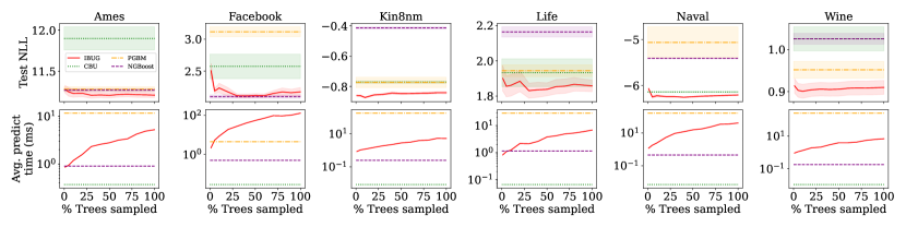
(b) Sampling trees first-to-last.

(c) Sampling trees last-to-first.

Figure 5: Probabilistic (NLL) performance (lower is better) and average prediction time (in milliseconds) per test example (lower is better) as a function of $\tau$ for different sampling techniques. Top: sample trees uniformly at random, middle: sample trees first-to-last (in terms of boosting iteration), bottom: sample trees last-to-first. All methods result in similar prediction times; however, first-to-last sampling typically provides the best NLL with the fewest number of trees sampled.

C.5 Leaf Density

Figure 6 shows the average percentage of train instances visited per tree as a function of the total number of training instances for each dataset. We note that for some datasets, CatBoost, LightGBM, and XGBoost induce regression trees with very dense leaves where over half the training instances belong to those leaves. Figure 7 shows average leaf density for each tree in the GBRT.

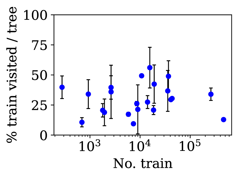
(a) CatBoost

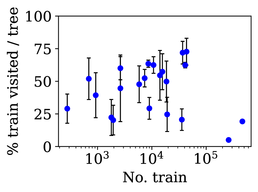
(b) LightGBM

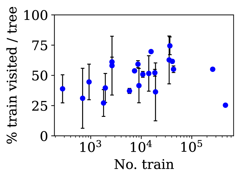
(c) XGBoost

Figure 6: Average percentage of training instances visited per tree while computing affinity vectors on the test set test for each dataset. Results are averaged over all test instances, and error bars represent standard deviation; lower is better. In general, the number of training instances visited per tree is highly dependent on the dataset; and for some datasets, is also highly dependent on the test example (points with large standard deviations).

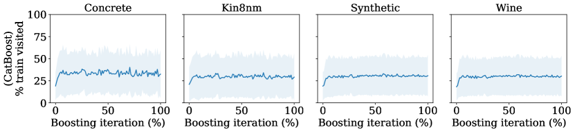
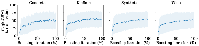
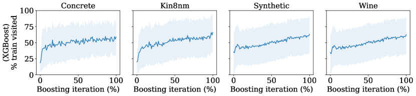
Figure 7: Average percentage of training instances visited at each iteration while computing affinity vectors on the test set for the Concrete, Kin8nm, Synthetic, and Wine datasets. Results are averaged over all test instances, and error bars represent standard deviation; lower is better. For LightGBM and XGBoost, weak learners later in training tend to pool a larger proportion of training instances into fewer leaves; in contrast, CatBoost has less dense leaves and training instances are more equally distributed among the leaves in each tree.

References

- Abu-Mostafa and Atiya [1996] Yaser S Abu-Mostafa and Amir F Atiya. Introduction to financial forecasting. Applied Intelligence, 6(3):205–213, 1996.
- Adadi and Berrada [2018] Amina Adadi and Mohammed Berrada. Peeking inside the black-box: A survey on explainable artificial intelligence (XAI). IEEE Access, 6:52138–52160, 2018.
- Alexandrov et al. [2020] Alexander Alexandrov, Konstantinos Benidis, Michael Bohlke-Schneider, Valentin Flunkert, Jan Gasthaus, Tim Januschowski, Danielle C Maddix, Syama Sundar Rangapuram, David Salinas, Jasper Schulz, et al. GluonTS: Probabilistic and neural time series modeling in python. Journal of Machine Learning Research, 21(116):1–6, 2020.
- Andrieu et al. [2003] Christophe Andrieu, Nando De Freitas, Arnaud Doucet, and Michael I Jordan. An introduction to MCMC for machine learning. Machine Learning, 50(1):5–43, 2003.
- Angelopoulos and Bates [2021] Anastasios N Angelopoulos and Stephen Bates. A gentle introduction to conformal prediction and distribution-free uncertainty quantification. arXiv preprint arXiv:2107.07511, 2021.
- Avati et al. [2018] Anand Avati, Kenneth Jung, Stephanie Harman, Lance Downing, Andrew Ng, and Nigam H Shah. Improving palliative care with deep learning. BMC Medical Informatics and Decision Making, 18(4):55–64, 2018.
- Bertin-Mahieux et al. [2011] Thierry Bertin-Mahieux, Daniel P.W. Ellis, Brian Whitman, and Paul Lamere. The million song dataset. In Proceedings of the 12th International Conference on Music Information Retrieval (ISMIR 2011), 2011.
- Bloniarz et al. [2016] Adam Bloniarz, Ameet Talwalkar, Bin Yu, and Christopher Wu. Supervised neighborhoods for distributed nonparametric regression. In Proceedings of the 18th International Conference on Artificial Intelligence and Statistics, pages 1450–1459, 2016.
- Böse et al. [2017] Joos-Hendrik Böse, Valentin Flunkert, Jan Gasthaus, Tim Januschowski, Dustin Lange, David Salinas, Sebastian Schelter, Matthias Seeger, and Yuyang Wang. Probabilistic demand forecasting at scale. In Proceedings of the VLDB Endowment, volume 10, pages 1694–1705. VLDB Endowment, 2017.
- Breiman [1996] Leo Breiman. Bagging predictors. Machine Learning, 24(2):123–140, 1996.
- Brophy and Lowd [2020] Jonathan Brophy and Daniel Lowd. Trex: Tree-ensemble representer-point explanations. In ICML Workshop on Extending Explainable AI, 2020.
- Chen and Guestrin [2016] Tianqi Chen and Carlos Guestrin. XGBoost: A scalable tree boosting system. In Proceedings of the 22nd ACM SIGKDD International Conference on Knowledge Discovery and Data Mining, 2016.
- Chipman et al. [2010] Hugh A Chipman, Edward I George, and Robert E McCulloch. BART: Bayesian additive regression trees. The Annals of Applied Statistics, 4(1):266–298, 2010.
- Chung et al. [2021] Youngseog Chung, Ian Char, Han Guo, Jeff Schneider, and Willie Neiswanger. Uncertainty toolbox: An open-source library for assessing, visualizing, and improving uncertainty quantification. arXiv preprint arXiv:2109.10254, 2021.
- Cohen et al. [2009] Joel W Cohen, Steven B Cohen, and Jessica S Banthin. The medical expenditure panel survey: A national information resource to support healthcare cost research and inform policy and practice. Medical Care, pages S44–S50, 2009.
- Coraddu et al. [2016] Andrea Coraddu, Luca Oneto, Aessandro Ghio, Stefano Savio, Davide Anguita, and Massimo Figari. Machine learning approaches for improving condition-based maintenance of naval propulsion plants. Journal of Engineering for the Maritime Environment, Part M, 230(1):136–153, 2016.
- Cortez et al. [2009] Paulo Cortez, António Cerdeira, Fernando Almeida, Telmo Matos, and José Reis. Modeling wine preferences by data mining from physicochemical properties. Decision Support Systems, 47(4):547–553, 2009.
- Davies and Ghahramani [2014] Alex Davies and Zoubin Ghahramani. The random forest kernel and other kernels for big data from random partitions. arXiv preprint arXiv:1402.4293, 2014.
- De Cock [2011] Dean De Cock. Ames, Iowa: Alternative to the Boston housing data as an end of semester regression project. Journal of Statistics Education, 19(3), 2011.
- D’souza et al. [2021] Daniel D’souza, Zach Nussbaum, Chirag Agarwal, and Sara Hooker. A tale of two long tails. arXiv preprint arXiv:2107.13098, 2021.
- Dua and Graff [2019] Dheeru Dua and Casey Graff. UCI machine learning repository. http://archive.ics.uci.edu/ml, 2019. [Online; accessed 12-September-2021].
- Duan et al. [2020] Tony Duan, Avati Anand, Daisy Yi Ding, Khanh K Thai, Sanjay Basu, Andrew Ng, and Alejandro Schuler. Ngboost: Natural gradient boosting for probabilistic prediction. In Proceedings of the 37th International Conference on Machine Learning, pages 2690–2700. PMLR, 2020.
- Fanaee-T and Gama [2013] Hadi Fanaee-T and Joao Gama. Event labeling combining ensemble detectors and background knowledge. Progress in Artificial Intelligence, pages 1–15, 2013.
- Fernandes et al. [2015] Kelwin Fernandes, Pedro Vinagre, and Paulo Cortez. A proactive intelligent decision support system for predicting the popularity of online news. In Proceedings of the 17th Portuguese Conference on Artificial Intelligence, pages 535–546. Springer, 2015.
- Ferreira and Monteiro [2020] Juliana J Ferreira and Mateus S Monteiro. What are people doing about XAI user experience? A survey on AI explainability research and practice. In Proceedings of the 22nd International Conference on Human-Computer Interaction, pages 56–73. Springer, 2020.
- Friedman et al. [2000] Jerome Friedman, Trevor Hastie, and Robert Tibshirani. Additive logistic regression: A statistical view of boosting. The Annals of Statistics, 28(2):337–407, 2000.
- Friedman [1991] Jerome H Friedman. Multivariate adaptive regression splines. The Annals of Statistics, pages 1–67, 1991.
- Gneiting and Katzfuss [2014] Tilmann Gneiting and Matthias Katzfuss. Probabilistic forecasting. Annual Review of Statistics and Its Application, 1:125–151, 2014.
- Gneiting and Raftery [2007] Tilmann Gneiting and Adrian E Raftery. Strictly proper scoring rules, prediction, and estimation. Journal of the American Statistical Association, 102(477):359–378, 2007.
- Graves [2011] Alex Graves. Practical variational inference for neural networks. In Proceedings of the 25th International Conference on Neural Information Processing Systems, volume 24, 2011.
- Hamidieh [2018] Kam Hamidieh. A data-driven statistical model for predicting the critical temperature of a superconductor. Computational Materials Science, 154:346–354, 2018.
- Hasson et al. [2021] Hilaf Hasson, Bernie Wang, Tim Januschowski, and Jan Gasthaus. Probabilistic forecasting: A level-set approach. In Proceedings of the 35th International Conference on Neural Information Processing Systems, volume 34, 2021.
- Hüllermeier and Waegeman [2021] Eyke Hüllermeier and Willem Waegeman. Aleatoric and epistemic uncertainty in machine learning: An introduction to concepts and methods. Machine Learning, 110(3):457–506, 2021.
- Januschowski et al. [2021] Tim Januschowski, Yuyang Wang, Kari Torkkola, Timo Erkkilä, Hilaf Hasson, and Jan Gasthaus. Forecasting with trees. International Journal of Forecasting, 2021.
- Kaya et al. [2012] Heysem Kaya, Pmar Tüfekci, and Fikret S Gürgen. Local and global learning methods for predicting power of a combined gas & steam turbine. In Proceedings of the 2nd International Conference on Emerging Trends in Computer and Electronics Engineering (ICETCEE), pages 13–18, 2012.
- Ke et al. [2017] Guolin Ke, Qi Meng, et al. LightGBM: A highly efficient gradient boosting decision tree. In Proceedings of the 31st International Conference on Neural Information Processing Systems, 2017.
- Koenker and Hallock [2001] Roger Koenker and Kevin F Hallock. Quantile regression. Journal of Economic Perspectives, 15(4):143–156, 2001.
- Li et al. [2019] Shiyang Li, Xiaoyong Jin, Yao Xuan, Xiyou Zhou, Wenhu Chen, Yu-Xiang Wang, and Xifeng Yan. Enhancing the locality and breaking the memory bottleneck of transformer on time series forecasting. In Proceedings of the 33rd International Conference on Neural Information Processing Systems, volume 32, pages 5243–5253, 2019.
- Lim et al. [2021] Bryan Lim, Sercan Ö Arık, Nicolas Loeff, and Tomas Pfister. Temporal fusion transformers for interpretable multi-horizon time series forecasting. International Journal of Forecasting, 2021.
- Lin and Jeon [2006] Yi Lin and Yongho Jeon. Random forests and adaptive nearest neighbors. Journal of the American Statistical Association, 101(474):578–590, 2006.
- Luo et al. [2021] Zhao Tang Luo, Huiyan Sang, and Bani Mallick. BAST: Bayesian additive regression spanning trees for complex constrained domain. In Proceedings of the 35th International Conference on Neural Information Processing Systems, volume 34, 2021.
- Makridakis et al. [2021] Spyros Makridakis, Evangelos Spiliotis, Vassilios Assimakopoulos, Zhi Chen, Anil Gaba, Ilia Tsetlin, and Robert L Winkler. The M5 uncertainty competition: Results, findings and conclusions. International Journal of Forecasting, 2021.
- Makridakis et al. [2022] Spyros Makridakis, Evangelos Spiliotis, and Vassilios Assimakopoulos. M5 accuracy competition: Results, findings, and conclusions. International Journal of Forecasting, 2022.
- Malinin et al. [2021] Andrey Malinin, Liudmila Prokhorenkova, and Aleksei Ustimenko. Uncertainty in gradient boosting via ensembles. In Proceedings of the 9th International Conference on Learning Representations, 2021.
- Meinshausen and Ridgeway [2006] Nicolai Meinshausen and Greg Ridgeway. Quantile regression forests. Journal of Machine Learning Research, 7(6), 2006.
- Moosmann et al. [2006] Frank Moosmann, Bill Triggs, and Frederic Jurie. Fast discriminative visual codebooks using randomized clustering forests. In Proceedings of the 20th International Conference on Neural Information Processing Systems, pages 985–992, 2006.
- Myung [2003] In Jae Myung. Tutorial on maximum likelihood estimation. Journal of Mathematical Psychology, 47(1):90–100, 2003.
- Neal [1996] Radford M Neal. Bayesian Learning for Neural Networks. Springer-Verlag, 1996.
- Pace and Barry [1997] R Kelley Pace and Ronald Barry. Sparse spatial autoregressions. Statistics & Probability Letters, 33(3):291–297, 1997.
- Peterson [2009] Leif E Peterson. K-nearest neighbor. Scholarpedia, 4(2):1883, 2009.
- Plumb et al. [2018] Gregory Plumb, Denali Molitor, and Ameet S Talwalkar. Model agnostic supervised local explanations. In Proceedings of the 32nd International Conference on Neural Information Processing Systems, pages 2515–2524, 2018.
- Prokhorenkova et al. [2018] Liudmila Prokhorenkova, Gleb Gusev, et al. CatBoost: Unbiased boosting with categorical features. In Proceedings of the 32nd International Conference on Neural Information Processing Systems, 2018.
- Rajarshi [2017] Kumar Rajarshi. Life expectancy (WHO). https://www.kaggle.com/kumarajarshi/life-expectancy-who?ref=hackernoon.com&select=Life+Expectancy+Data.csv, 2017. [Online; accessed 12-September-2021].
- Rangapuram et al. [2018] Syama Sundar Rangapuram, Matthias W Seeger, Jan Gasthaus, Lorenzo Stella, Yuyang Wang, and Tim Januschowski. Deep state space models for time series forecasting. In Proceedings of the 32nd International Conference on Neural Information Processing Systems, volume 31, pages 7785–7794, 2018.
- Redmond and Baveja [2002] Michael Redmond and Alok Baveja. A data-driven software tool for enabling cooperative information sharing among police departments. European Journal of Operational Research, 141(3):660–678, 2002.
- Rigby and Stasinopoulos [2005] Robert A Rigby and D Mikis Stasinopoulos. Generalized additive models for location, scale and shape. Journal of the Royal Statistical Society: Series C (Applied Statistics), 54(3):507–554, 2005.
- Romano et al. [2019] Yaniv Romano, Evan Patterson, and Emmanuel Candes. Conformalized quantile regression. In Proceedings of the 33rd International Conference on Neural Information Processing Systems, volume 32, pages 3543–3553, 2019.
- Salinas et al. [2020] David Salinas, Valentin Flunkert, Jan Gasthaus, and Tim Januschowski. Deepar: Probabilistic forecasting with autoregressive recurrent networks. International Journal of Forecasting, 36(3):1181–1191, 2020.
- Schlosser et al. [2019] Lisa Schlosser, Torsten Hothorn, Reto Stauffer, and Achim Zeileis. Distributional regression forests for probabilistic precipitation forecasting in complex terrain. The Annals of Applied Statistics, 13(3):1564–1589, 2019.
- Sen et al. [2019] Rajat Sen, Hsiang-Fu Yu, and Inderjit Dhillon. Think globally, act locally: A deep neural network approach to high-dimensional time series forecasting. In Proceedings of the 33rd International Conference on Neural Information Processing Systems, pages 4837–4846, 2019.
- Shafer and Vovk [2008] Glenn Shafer and Vladimir Vovk. A tutorial on conformal prediction. Journal of Machine Learning Research, 9(3), 2008.
- Sheather and Jones [1991] Simon J Sheather and Michael C Jones. A reliable data-based bandwidth selection method for kernel density estimation. Journal of the Royal Statistical Society: Series B (Methodological), 53(3):683–690, 1991.
- Singh et al. [2015] Kamaljot Singh, Ranjeet Kaur Sandhu, and Dinesh Kumar. Comment volume prediction using neural networks and decision trees. In IEEE UKSim-AMSS 17th International Conference on Computational Modeling and Simulation, UKSim2015, March 2015.
- Sprangers et al. [2021] Olivier Sprangers, Sebastian Schelter, and Maarten de Rijke. Probabilistic gradient boosting machines for large-scale probabilistic regression. In Proceedings of the 27th ACM SIGKDD Conference on Knowledge Discovery & Data Mining, 2021.
- Stock et al. [2012] James H Stock, Mark W Watson, et al. Introduction to Econometrics, volume 3. Pearson New York, 2012.
- Suzanne [2018] Suzanne. CDC data: Nutrition, physical activity, & obesity. https://www.kaggle.com/spittman1248/cdc-data-nutrition-physical-activity-obesity, 2018. [Online; accessed 12-September-2021].
- Taieb et al. [2015] Souhaib Ben Taieb, Raphael Huser, Rob Hyndman, Marc Genton, et al. Probabilistic time series forecasting with boosted additive models: An application to smart meter data. Department of Economics and Business Statistics, Monash University, 2015.
- Taylor and Letham [2018] Sean J Taylor and Benjamin Letham. Forecasting at scale. The American Statistician, 72(1):37–45, 2018.
- Tjoa and Guan [2020] Erico Tjoa and Cuntai Guan. A survey on explainable artificial intelligence (XAI): Toward medical XAI. IEEE Transactions on Neural Networks and Learning Systems, 2020.
- Tsanas and Xifara [2012] Athanasios Tsanas and Angeliki Xifara. Accurate quantitative estimation of energy performance of residential buildings using statistical machine learning tools. Energy and Buildings, 49:560–567, 2012.
- Tüfekci [2014] Pınar Tüfekci. Prediction of full load electrical power output of a base load operated combined cycle power plant using machine learning methods. International Journal of Electrical Power & Energy Systems, 60:126–140, 2014.
- Ustimenko and Prokhorenkova [2021] Aleksei Ustimenko and Liudmila Prokhorenkova. SGLB: Stochastic gradient langevin boosting. In International Conference on Machine Learning, pages 10487–10496. PMLR, 2021.
- van Rijn [2014] Jan van Rijn. Kin8nm. https://www.openml.org/d/189, 2014. [Online; accessed 20-January-2022].
- Wang et al. [2019] Yuyang Wang, Alex Smola, Danielle Maddix, Jan Gasthaus, Dean Foster, and Tim Januschowski. Deep factors for forecasting. In Proceedings of the 36th International Conference on Machine Learning, pages 6607–6617. PMLR, 2019.
- Yeh [1998] I-C Yeh. Modeling of strength of high-performance concrete using artificial neural networks. Cement and Concrete Research, 28(12):1797–1808, 1998.
- Zamo and Naveau [2018] Michaël Zamo and Philippe Naveau. Estimation of the continuous ranked probability score with limited information and applications to ensemble weather forecasts. Mathematical Geosciences, 50(2):209–234, 2018.