citenum
Causal Machine Learning
for Healthcare and Precision Medicine
Abstract
Causal machine learning (CML) has experienced increasing popularity in healthcare. Beyond the inherent capabilities of adding domain knowledge into learning systems, CML provides a complete toolset for investigating how a system would react to an intervention (e.g. outcome given a treatment). Quantifying effects of interventions allows actionable decisions to be made whilst maintaining robustness in the presence of confounders. Here, we explore how causal inference can be incorporated into different aspects of clinical decision support (CDS) systems by using recent advances in machine learning. Throughout this paper, we use Alzheimer’s disease (AD) to create examples for illustrating how CML can be advantageous in clinical scenarios. Furthermore, we discuss important challenges present in healthcare applications such as processing high-dimensional and unstructured data, generalisation to out-of-distribution samples, and temporal relationships, that despite the great effort from the research community remain to be solved. Finally, we review lines of research within causal representation learning, causal discovery and causal reasoning which offer the potential towards addressing the aforementioned challenges.
1 Introduction
Considerable progress has been made in predictive systems for medical imaging following the advent of powerful machine learning (ML) approaches such as deep learning (Litjens et al., 2017). In healthcare, clinical decision support (CDS) tools make predictions for tasks such as detection, classification and/or segmentation from electronic health record (EHR) data such as medical images, clinical free-text notes, blood tests, and genetic data. These systems are usually trained with supervised learning techniques. However, most CDS systems powered by ML techniques learn only associations between variables in the data, without distinguishing between causal relationships and (spurious) correlations.
CDS systems targeted at precision medicine (also known as personalised medicine) need to answer complex queries about how individuals would respond to interventions. A precision CDS system for Alzheimer’s disease (AD), for instance, should be able to quantify the effect of treating a patient with a given drug on the final outcome, e.g. predict the subsequent cognitive test score. Even with the appropriate data and perfect performance, current ML systems would predict the best treatment based only on previous correlations in data, which may not represent actionable information. Information is defined as actionable when it enables treatment (interventional) decisions to be based on a comparison between different scenarios (e.g. outcomes for treated vs not treated) for a given patient. Such systems need causal inference (CI) in order to make actionable and individualised treatment effect predictions (Bica et al., 2021).
A major upstream challenge in healthcare is how to acquire the necessary information to causally reason about treatments and outcomes. Modern healthcare data is multimodal, high-dimensional and often unstructured. Information from medical images, genomics, clinical assessments, and demographics must be taken into account when making predictions. A multimodal approach better emulates how human experts use information to make predictions. In addition, many diseases are progressive over time, thus necessitating that time (the temporal dimension) is taken into account. Finally, any system must ensure that these predictions will be generalisable across deployment environments such as different hospitals, cities, or countries.
Interestingly, it is the connection between causal inference and machine learning that can help alleviate these challenges. ML allows causal models to process high-dimensional and unstructured data by learning complex non-linear relations between variables. CI adds an extra layer of understanding about a system with expert knowledge, which improves information merging from multimodal data, generalisation, and explainability of current ML systems.
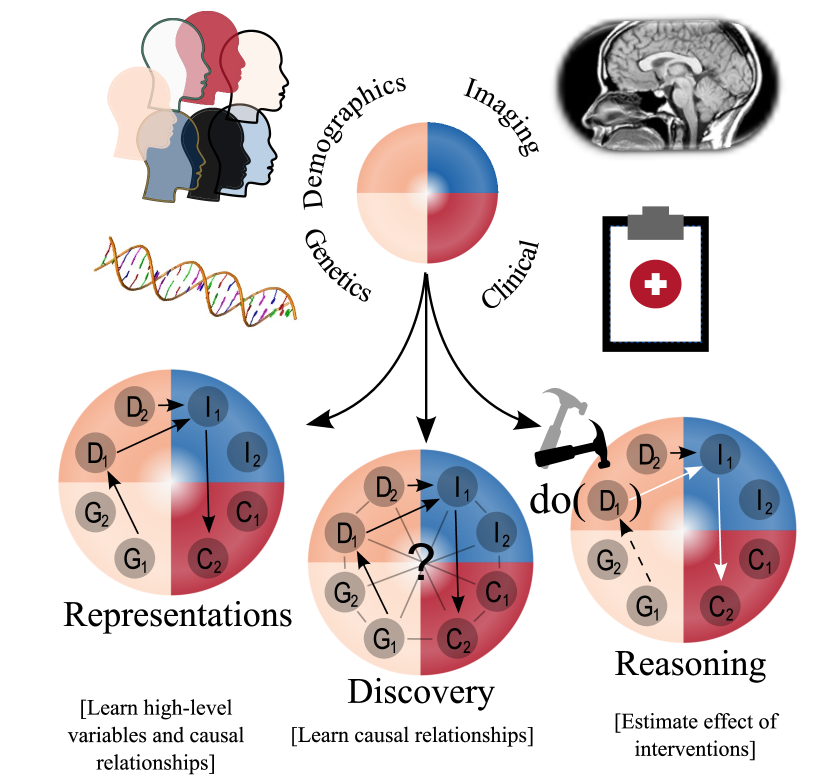
The causal machine learning (CML) literature offers several directions for addressing the aforementioned challenges when using observational data. Here, we categorise CML into three directions: (i) Causal Representation Learning– given high-dimensional data, learn to extract low-dimensional informative (causal) variables and their causal relations; (ii) Causal Discovery– given a set of variables, learn the causal relationships between them; and (iii) Causal Reasoning– given a set of variables and their causal relationships, analyse how a system will react to interventions. These directions are illustrated in Fig. 1.
In this paper, we discuss how CML can improve personalised decision making as well as help to mitigate pressing challenges in clinical decision support systems. We review representative methods for CML, explaining how they can be used in a healthcare context. In particular, we (i) present the concept of causality and causal models; (ii) show how they can be useful in healthcare settings; (iii) discuss pressing challenges; and (iv) review potential research directions from CML.
2 What is causality?
We use a broad definition of causality: if is a cause and is an effect, then relies on for its value. As causal relations are directional, the reverse is not true; does not rely on for its value. The notion of causality thus enables analysis of how a system would respond to an intervention.
Questions such as “How will this disease progress if a patient is given treatment X?” or “Would this patient still have experienced outcome Z if treatment Y was received?” require methods from causality to understand how an intervention would affect a specific individual. In a clinical environment, causal reasoning can be useful for deciding which treatment will result in the best outcome. For instance, in an AD scenario, causality can answer queries such as “Which of drug or drug would best minimise the patient’s expected cognitive decline within a 5 year time span?”. Ideally, we would compare the outcomes of alternative treatments using observational (historical) data. However, the “fundamental problem of causal inference” (Holland, 1986) is that for each unit (i.e. patient) we can observe either the result of treatment or of treatment , but never both at the same time. This is because after making a choice on a treatment, we cannot turn back time to undo the treatment. These queries that entertain hypothetical scenarios about individuals are called potential outcomes. Thus, we can observe only one of the potential consequences of an action; the unobserved quantity becomes a counterfactual. Causality’s mathematical formalism pioneered by Judea Pearl (Pearl, 2009) and Donald Rubin (Imbens and Rubin, 2015) allows these more challenging queries to be answered.
Most machine learning approaches are not (currently) able to identify cause and effect, because causal inference is fundamentally impossible to achieve without making assumptions (Pearl, 2009; Peters et al., 2017). Several of these assumptions can be satisfied through study design or external contextual knowledge, but none can be discovered solely from observational data.
Next, we introduce the reader to two ways of defining and reasoning about causal relationships: with structural causal models and with potential outcomes. We wrap up this section with an introduction to determining causal relationships, including the use of randomised controlled trials.
2.1 Structural Causal Models
The mathematical formalism around the so-called do-calculus and structural causal models (SCMs) pioneered by the Turing Award winner Judea Pearl (Pearl, 2009) has allowed a graphical perspective to reasoning with data which heavily relies on domain knowledge. This formalism can model the data generation process and incorporate assumptions about a given problem. An intuitive and historical description of causality can be found in Pearl and Mackenzie (2018)’s recent book The Book of Why.
An SCM consists of a collection of structural assignments (called mechanisms)
| (1) |
where is the set of parent variables of (its direct causes) and is a noise variable for modeling uncertainty. is also referred to as exogenous noise because it represents variables that were not included in the causal model, as opposed to the endogenous variables which are considered known or at least intended by design to be considered, and from which the set of parents are drawn. This model can be defined as a direct acyclic graph (DAG) in which the nodes are the variables and the edges are the causal mechanisms. One might consider other graphical structures which incorporate cycles and latent variables (Bongers et al., 2021), depending on the nature of the data.
It is important to note that the causal mechanisms are representations of physical mechanisms that are present in the real world. Therefore, according to the principle of independent causal mechanisms (ICM), we assume that the causal generative process of a system’s variables is composed of autonomous modules that do not inform or influence each other (Peters et al., 2017; Schölkopf et al., 2021). This means that exogenous variables are mutually independent with the following joint distribution . Moreover, the joint distribution over the endogenous variables can be factorised as a product of independent conditional mechanisms
| (2) |
The causal framework now allows us to go beyond (i) associative predictions, and begin to answer (ii) interventional and (iii) counterfactual queries. These three tasks are also known as Pearl’s causal hierarchy (Pearl and Mackenzie, 2018). The do-calculus introduces the notation , to denote a system where we have intervened to fix the value of . This allows us to sample from an interventional distribution , which has the advantage over an observational distribution that the causal structure enforces that only the descendants of the variable intervened upon will be modified by a given action.
2.2 Potential Outcomes
An alternative approach to causal inference is the potential outcomes framework proposed by Rubin (2005). In this framework, a response variable is used to measure the effect of some cause or treatment for a patient, . The value of may be affected by the treatment assigned to . To enable the treatment effect to be modelled, we represent the response with two variables and which denote “untreated” and “treated” respectively. The effect of the treatment on is then the difference, .
As a patient may potentially be untreated or treated, we refer to and as potential outcomes. It is, however, impossible to observe both simultaneously, according to the previously mentioned fundamental problem of causal inference (Holland, 1986). This does not mean that causal inference itself is impossible, but it does bring challenges (Imbens and Rubin, 2015). Causal reasoning in the potential outcome frameworks depends on obtaining an estimate for the joint probability distribution, .
Both SCM and potential outcomes approaches have useful applications, and are used where appropriate throughout this article. We note that single world intervention graphs (Richardson and Robins, 2013) have been proposed as a way to unify them.
2.3 Determining Cause and Effect
Determining causal relationships often requires carefully designed experiments. There is a limit to how much can be learned using purely observational data.
The effects of causes can be determined through prospective experiments to observe an effect after a cause is tried or withheld, keeping constant all other possible factors. It is hard, and in most cases impossible, to control for all possible confounders of and . The gold standard for discovering a true causal effect is by performing a randomised controlled trial (RCT), where the choice of is randomised, thus removing confounding. For example, by randomly assigning a drug or a placebo to patients participating in an interventional study, we can measure the effect of the treatment, eliminating any bias that may have arisen in an observational study due to other confounding variables, such as lifestyle factors, that influence both the choice of using the drug and the impact of cognitive decline (Mangialasche et al., 2010).
Note that the conditional probability of observing after observing can be different from the interventional probability of observing after doing / intervening on . means that only the descendants of (in a causal graph) change after an intervention, all other variables maintain their values. In RCTs, the ‘’ is guaranteed and unconditioned, while with observational data such as historical Electronic Health Records (EHRs), it is not, due to the presence of confounders.
Determining the causes of effects (the aetiology of diseases) requires hypotheses and experimentation where interventions are performed and studied to determine the necessary and sufficient conditions for an effect or disease to occur.
3 Why should we consider a causal framework in healthcare?
Causal inference has made several contributions over the last few decades to fields such as social sciences, econometrics, epidemiology, and aetiology (Pearl, 2009; Imbens and Rubin, 2015), and it has recently spread to other healthcare fields such as medical imaging (Castro et al., 2020; Pawlowski et al., 2020; Reinhold et al., ) and pharmacology (Bica et al., 2021). In this section, we will elaborate on how causality can be used for improving medical decision making.
Even though data from EHRs, for example, are usually observational, they have already been successfully leveraged in several machine learning applications (Piccialli et al., 2021), such as modeling disease progression (Lim, 2018a), predicting disease deterioration (Tomašev et al., 2019), and discovering risk factors (McCauley and Darbar, 2016), as well as for predicting treatment responses (Athreya et al., 2019). Further, we now have evidence of algorithms which achieve superhuman performance in imaging tasks such as segmentation (Isensee et al., 2021), detection of pathologies and classification (Korot et al., 2021). However, predicting a disease with almost perfect accuracy for a given patient is not what precision medicine is trying to achieve (Wilkinson et al., 2020). Rather, we aim to build machine learning methods which extract actionable information from observational patient data in order to make interventional (treatment) decisions. This requires causal inference, which goes beyond standard supervised learning methods for prediction as detailed below.
In order to make actionable decisions at the patient level, one needs to estimate the treatment effect. The treatment effect is the difference between two potential outcomes: the factual outcome and the counterfactual outcome. For actionable predictions, we need algorithms that learn how to reason about hypothetical scenarios in which different actions could have been taken, creating, therefore, a decision boundary that can be navigated in order to improve patient outcome. There is recent evidence that humans use counterfactual reasoning to make causal judgements (Gerstenberg et al., 2021), lending support to this reasoning hypothesis.
This is what makes the problem of inferring treatment effect fundamentally different from standard supervised learning (Bica et al., 2021) as defined by the potential outcome framework (Rubin, 2005; Imbens and Rubin, 2015). When using observational datasets, by definition, we never observe the counterfactual outcome. Therefore, the best treatment for an individual – the main goal of precision medicine (Zhang et al., 2018) – can only be identified with a model that is capable of causal reasoning as will be detailed in Section 3.3.
3.1 Alzheimer’s Disease practical example
We now illustrate the notion of causal machine learning for healthcare with an example from Alzheimer’s disease (AD). A recent attempt to understand AD from a causal perspective (Shen et al., 2020; Uleman et al., 2020) takes into account many biomarkers and uses domain knowledge (as opposed to RCTs) for deriving ground truth causal relationships. In this section, we present a simpler view with only three variables: chronological age111Age can otherwise be measured in biological terms using, for instance, DNA methylation (Horvath, 2013)., magnetic resonance (MR) images of the brain, and Alzheimer’s disease diagnosis. The diagnosis of Alzheimer’s disease is made by a clinician who takes into account all available clinical information, including images. We are particularly interested in MR images because analysing the relationship of high-dimensional data such as medical images, is a task that can be more easily handled with machine learning techniques, the main focus of this paper.
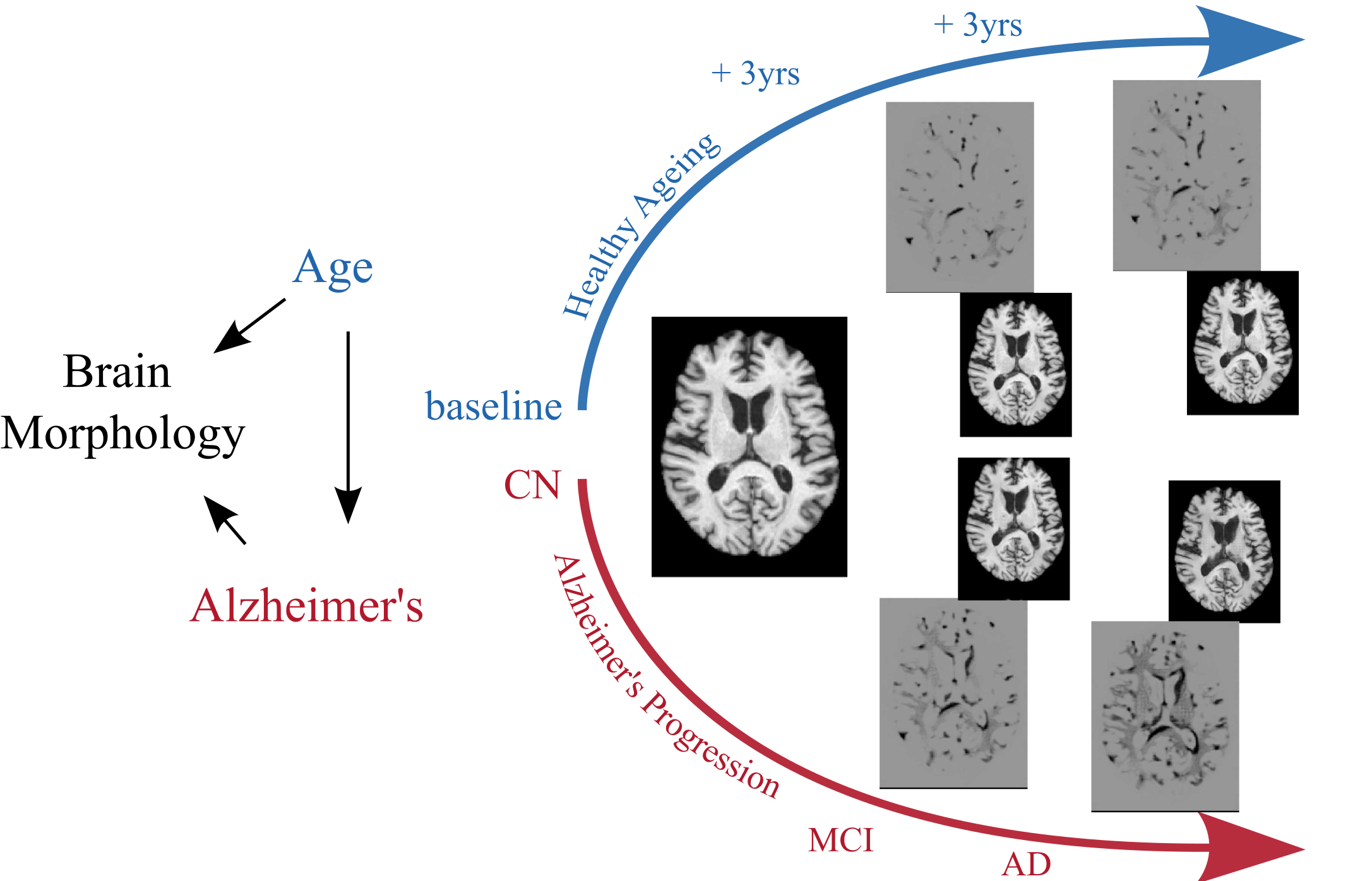
AD is a type of cognitive decline that generally appears later in life (Jack et al., 2015). Alzheimer’s disease is associated with brain atrophy (Karas et al., 2004; Qian et al., 2019) i.e. volumetric reduction of grey matter. We consider that Alzheimer’s disease causes the symptom of brain morphology change, following Richens et al. (2020), by arguing that a high-dimensional variable such as the MR image is caused by the factors that generated it; this modelling choice has been previously used in the causality literature (Schölkopf et al., 2012; Kilbertus et al., 2018; Heinze-Deml and Meinshausen, 2021). Further, it is well established that atrophy also occurs during normal ageing (Sullivan et al., 1995; Good et al., 2001). Time does not depend on any biological variable, therefore chronological age cannot be caused by Alzheimer’s disease nor any change in brain morphology. In this scenario, we can assume that age is a confounder of brain morphology, measured by the MR image, and Alzheimer’s disease diagnosis. These relationships are illustrated in the causal graph in Fig. 2.
To model the effect of having age as a confounder of brain morphology and Alzheimer’s disease, we use a conditional generative model from Xia et al. (2021)222We take the model from Xia et al. (2021) and run new demonstrative experiments for illustration in this paper., in which we condition on age and Alzheimer’s disease diagnosis for brain MRI image generation. We then synthesise images of a patient at different ages and with different Alzheimer’s disease status as depicted in Fig. 2. In particular, we control for (i.e. condition on) one variable while intervening on the other. That is, we synthesise images based on a patient who is cognitively normal (CN) for their age of 64 years. We then fix the Alzheimer’s status at CN and increase the age by 3 years for 3 steps, resulting in images of the same CN patient at ages 64, 67, 70, 73. At the same time, we synthesise images with different Alzheimer’s status by fixing the age at 64 and changing the Alzheimer’s status from mild cognitive impairment (MCI) to a clinical diagnosis of Alzheimer’s disease (AD).
This example illustrates the effect of confounding bias. By observing qualitatively the difference between the baseline and synthesised images, we see that ageing and Alzheimer’s disease have similar effects on the brain333See Xia et al. (2021) for quantitative results confirming this hypothesis.. That is, that both variables change the volume of brain when intervened on independently.
Throughout the paper, we will further add variables and causal links to this example to illustrate how healthcare problems can become more complex and how a causal approach might mitigate some of the main challenges. In particular, we will build on this example by explaining some consequences of causal modelling for dealing with high-dimensional and unstructured data, generalisation and temporal information.
3.2 Modeling the Data Generation Process
The Alzheimer’s disease example illustrates the importance of considering causal relationships in a machine learning scenario. Namely, causality gives the ability to model and identify types and sources of bias444we refer to https://catalogofbias.org/biases for a catalogue of bias types. To correctly identify which variables to control for (as means to mitigate confounding bias), causal diagrams (Pearl, 2009) offer a direct means of visual exploration and consequently explanation (Brookhart et al., 2010; Lederer et al., 2019).
Castro et al. (2020) details further how understanding the causal generating process can be useful in medical imaging. By representing the variables of a particular problem and their causal relationships as a causal graph, one can model domain shifts such as population shift (different cohorts), acquisition shift (different sites or scanners) and annotation shift (different annotators), and data scarcity (imbalanced classes).
In the Alzheimer’s disease setting above, a classifier naively trained to perform diagnosis from MR images of the brain might focus on the brain atrophy alone. This classifier may show reduced performance in younger adults with Alzheimer’s disease or for cognitively normal older adults, leading to potentially incorrect diagnosis. To illustrate this, we report the results of a convolutional neural network (CNN) classifier trained and tested on the ADNI dataset following the same setting as Xia et al. (2022)555Although we replicate results from Xia et al. (2022), this work does not constitute an extension of the original paper. Rather, we use Xia et al. (2022) as an example that illustrates how causality might impact standard machine learning.. Table 1 shows that as feared, healthy older patients (80-90 years old) are less accurately predicted because ageing itself causes the brain to have Alzheimer’s-like patterns.
| Age Range (years) | 60-70 | 70-80 | 80-90 | |
|---|---|---|---|---|
| Precision | 87.7 | 91.4 | 75.5 | |
| Naive | Recall | 92.5 | 94.2 | 97.1 |
| Precision | 88.3 | 93.6 | 84.2 | |
| Counterfactually Augmented | Recall | 91.5 | 96.5 | 95.7 |
Indeed, using augmented data based on causal knowledge is a solution discussed in Xia et al. (2022), whereby the training data are augmented with counterfactual images of a patient when intervening on age. That is, images of a patient at different ages (while controlling for Alzheimer’s status) are synthesised so the classifier learns how to differentiate the effects of ageing vs Alzheimer’s disease in brain images.
This causal knowledge enables the formulation of best strategies for mitigating data bias(es) and improving generalisation (further detailed in Section 4.3). For example, if after modeling the data distribution, an acquisition shift becomes apparent (e.g. training data were obtained with a specific MR sequence but the model will be evaluated on data from a different sequence), then data augmentation strategies can be designed to increase robustness of the learned representation. The acquisition shift – e.g. different intensities due to different scanners – might be modeled according to the physics of the (sensing) systems. Ultimately, creating a diagram of the data generation process helps rationalise/visualise which are the best strategies to solve the problem.
3.3 Treatment Effect and Precision Medicine
Beyond diagnosis, a major challenge in healthcare is ascertaining whether a given treatment influences an outcome. For a binary treatment decision, for instance, the aim is to estimate the average treatment effect (ATE), where is the outcome given the treatment and is the outcome without it (control). As it is impossible to observe both potential outcomes and for a given patient , this is typically estimated using , where is the treatment assignment.
The treatment assignment and outcomes, however, both depend on the patient’s condition in normal clinical conditions. This results in confounding, which is best mitigated by the use of an RCT 2.3. Performing an RCT as detailed in Section 2.3, however, is not always feasible, and causal inference techniques can be used to estimate the causal effect of treatment from observational data (Meid et al., 2020). A number of assumptions need to hold in order for the treatment effect to be identifiable from observational data (Lesko et al., 2017; Imbens and Rubin, 2015). Conditional exchangeability (ignorability) assumes there are no unmeasured confounders. Positivity (overlap) is the assumption that every patient has a chance of receiving each treatment. Consistency assumes that the treatment is defined unambiguously. Continuing the Alzheimer’s example, Charpignon et al. (2021) explore drug re-purposing by emulating an RCT with a target trial (Hernán and Robins, 2016) and find indications that metformin (a drug classically used for diabetes) might prevent dementia.
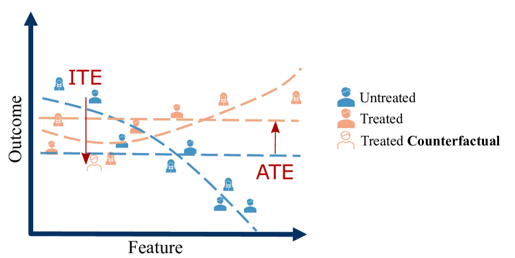
Note that even if the treatment effect is estimated using data from a well-designed RCT, is the average treatment effect across the study population. However, there is evidence (Bica et al., 2021) that for any given treatment, it is likely that only a small proportion of subjects will actually respond in a manner that resembles the “average” patient, as illustrated in Fig. 3. In other words, the treatment effect can be highly heterogeneous across a population. The aim of precision medicine is to determine the best treatment for an individual (Wilkinson et al., 2020), rather than simply measuring the average response across a population. In order to answer this question for a binary treatment decision, it is necessary to estimate for a patient . This is known as the individualised treatment effect (ITE). As this estimation is performed using a conditional average, this is also referred to as the conditional average treatment effect (CATE) (Abrevaya et al., 2015).
A number of approaches have been proposed to learn conditional average treatment effect from observational data, such as estimating treatment effect with double machine learning (Chernozhukov et al., 2018; Semenova and Chernozhukov, 2020). Another trend for estimating CATE are based on meta-learners (Künzel et al., 2019; Curth and Schaar, 2021). In the meta-learning setting, traditional (supervised) machine learning is used to predict the conditional expectations of outcome for units under control and under treatment separately. Then, CATE is done by taking the difference between the estimates of these estimates. While most approaches concentrate on estimating CATE using observational data, it is also possible to do so using data from an RCT (Hoogland et al., 2021).
A long-term goal of precision medicine (Bica et al., 2021) includes personalised risk assessment and prevention. Without a causal model to distinguish these questions from simpler prediction systems, interpretational mistakes will arise. In order to design more robust and effective machine learning methods for personalised treatment recommendations, it is vital that we gain a deeper theoretical understanding of the challenges and limitations of modeling multiple treatment options, combinations, and treatment dosages from observational data.
4 Causal machine learning for complex data
In Section 3, we focused on causal reasoning in situations where the causal models are known (at least partially) and variables are well demarcated. We refer the reader to Bica et al. (2021) for a comprehensive review on these methods. Most healthcare problems, however, have challenges that are upstream of causal reasoning. In this section, we highlight the need to deal with high-dimensional and multimodal data as well as with temporal information and discuss generalisation in out-of-distribution settings when learning from unstructured data.
4.1 Multimodal Data
Alzheimer’s disease, in common with other major diseases such as diabetes and cancer, has multiple causes arising from complex interactions between genetic and environmental factors. Indeed, a recent attempt (Shen et al., 2020) to build causal graphs for describing Alzheimer’s disease takes into account data derived from several data sources and modalities, including patient demographics, clinical measurements, genetic data, and imaging exams. Uleman et al. (2020), in particular, creates a causal graph 666Interestingly, Uleman et al. (2020) gather expert knowledge using a group model-building technique (Vennix and Forrester, 1999) where multiple experts with complementary skills create a graph based on their combined mental models and assumptions. with clusters of nodes related to brain health, physical health, and psychosocial health, illustrating the complexity of AD.
The above example illustrates that modern healthcare is multimodal. New ways of measuring biomarkers are increasingly accessible and affordable, but integrating this information is not trivial. Information from different sources needs to be transformed to a space where information can be combined, and the common information across modalities needs to be disentangled from the unique information within each modality (Braman et al., 2021). This is critical for developing CDS systems capable of integrating images, text and genomics data.
On the other hand, the availability of more variables might mean that some assumptions which are made in classical causal inference are more realistic. In particular, most methods consider the assumption of conditional exchangeability (or causal sufficiency (Spirtes et al., 2000)), as in section 3 3.3. In practice, the conditional exchangeability assumption may often not be true due to the presence of unmeasured confounders. However, observing more variables might reduce the probability of this, rendering the assumption more plausible.
4.2 Temporal Data
It is well known that a gene called apolipoprotein E (APOE) is associated with an increased risk of AD (Zlokovic, 2013; Mishra et al., 2018). However, environmental factors, such as education (Stern et al., 1994; Larsson et al., 2017; Anderson et al., 2020), also have an impact on dementia. In other words, environmental factors over time contribute to different disease trajectories in Alzheimer’s disease. In addition, there are possible loops in the causal diagram (Uleman et al., 2020). Wang and Holtzman (2019) illustrate, for instance, a positive feedback loop between sleep and AD. That is, poor sleep quality aggravates amyloid-beta and tau pathology concentrations, potentially leading to neuronal dysfunction which, in turn, leads to worse sleep quality. It is, therefore, important to consider data-driven approaches for understanding and modeling the progression of disease over time (Oxtoby and Alexander, 2017).
At the same time, using temporal information for inferring causation can be traced back to one of the first definitions of causality by Hume (1904). Quoting Hume: “we may define a cause to be an object followed by another, and where all the objects, similar to the first, are followed by objects similar to the second”. There are many strategies for incorporating time into causal models since using SCMs with directed acyclic graphs (as defined in Section 2 2.1) is not enough in this context. A classical model of causality for time-series was developed by Granger (1969). Granger considers if past is predictive of future . Therefore, inferring causality from time series data is at the core of CML. Bongers et al. (2021) shows that SCMs can be defined with latent variables and cycles, allowing temporal relationships. Early work has used temporal causal inference in neuroscience (Friston et al., 2003), but the application of temporal causal inference in combination with machine learning for understanding and dealing with complex disease remains largely unexplored.
Managing diseases such as Alzheimer’s disease can be challenging due to the heterogeneity of symptoms and their trajectory over time across the population. A pathology might evolve differently for patients with different covariates. For treatment decisions in a longitudinal setting, causal inference methods need to model patient history and treatment timing (Soleimani et al., 2017). Estimating trajectories under different possible future treatment plans (interventions) is extremely important (Bica et al., 2020). CDS systems need to take into account the current health state of the patient, to make predictions about the potential outcomes for hypothetical future treatment plans, to enable decision-makers to choose the sequence and timing of treatments that will lead to the best patient outcome (Lim, 2018b; Bica et al., 2020; Li et al., 2021).
4.3 Out-of-Distribution Generalisation with Unstructured and High-Dimensional Data
The challenge of integrating different modalities and temporal information increases when unstructured data is used. Most causality theory was originally developed in the context of epidemiology, econometrics, social sciences, and other fields wherein the variables of interest tend to be scalars (Pearl, 2009; Imbens and Rubin, 2015). In healthcare, however, the use of imaging exams and free-text reports poses significant challenges for consistent and robust extraction of meaningful information. The processing of unstructured data is mostly tackled with machine learning, and generalisation is one of the biggest challenges for learning algorithms.
In its most basic form, generalisation is the ability to correctly categorise new samples that differ from those used for training (Bishop and Nasrabadi, 2006). However, when learning from data, the notion of generalisation has many facets. Here, we are interested in a realistic setting where the test data distribution might be different from the training data distribution. This setting is often referred as out-of-distribution (OOD) generalisation. Distribution shifts are often caused by a change in environment (e.g. different hospitals). We wish to present a causal perspective (Gong et al., 2016; Rojas-Carulla et al., 2018; Meinshausen, 2018) on generalisation which unifies many machine learning settings. Causal relationships are stable across different environments (Cui and Athey, 2022). In a causal learning, the prediction should be invariant to distribution shifts (Peters et al., 2016a).
As the use of machine learning in high impact domains becomes widespread, the importance of evaluating safety has increased. A key aspect is evaluating how robust a model is to changes in environment (or domain), which typically requires applying the model to multiple independent datasets (Subbaswamy et al., 2021). Since the cost of collecting such datasets is often prohibitive, causal inference argues that providing structure (which comes from expert knowledge) is essential for increasing robustness in real life (Pearl, 2009).
Imagine a prediction problem where the goal is to learn , with the causal graph illustrated in Fig. 4. We consider an environment variable which controls the relationship between and . is a confounder and is caused by the two variables .
Firstly, we consider the view that most prediction problems are in the anti-causal direction (Schölkopf et al., 2012; Kilbertus et al., 2018; Heinze-Deml and Meinshausen, 2021; Rosenfeld et al., 2021)777We note that other seminal works (Peters et al., 2016b; Arjovsky et al., 2019) consider prediction a causal task because prediction should copy a cognitive human process of generating labels given the data.. That is, when making a prediction from a high-dimensional, unstructured variable (e.g. a brain image) one is usually interested in extracting and/or categorising one of its true generating factors (e.g. gray matter volume). , which represents the causal mechanism, , is independent of , however is not as . Thus changes as the environment changes.
Secondly, another (or many others) generating factor is often correlated with , which might cause the predictor to learn the relationship between and instead of the . This is known as shortcut learning (Geirhos et al., 2020) as it may be easier to learn the spurious correlation than the required relationship. For example, suppose an imaging dataset is collected from two hospitals, and . Hospital has a large neurological disorder unit, hence a higher prevalence of AD status (denoted by ), and uses a 3T MRI scanner (scanner type denoted by ). Hospital with no specialist unit, hence a lower prevalence of AD, happens to use a more common 1.5T MRI scanner. The model will learn the spurious correlation between (scanner type) and (AD status).

We can now describe several machine learning settings based on this causal perspective by comparing data availability at train and test time. Classical supervised learning (or empirical risk minimisation (ERM) (Vapnik, 1999)) uses the strong assumption that the data from train and test sets are independent and identically distributed (i.i.d.), therefore we assign the same environment for both sets. Semi-supervised learning (Chapelle et al., 2009) is a case where part of the training samples are not paired to annotations. Continual (or Lifelong) learning considers the case where data from different environments are added after training, and the challenge is to learn new environments without forgetting what has initially been learned. In domain adaptation, only unpaired data from the test environment is available during training. Domain generalisation aims at learning how to become invariant to changes of environment, such that a new (unseen in training data) environment can be used for the test set. Enforcing fairness is important when is a sensitive variable and the train set has and spuriously888We use the term spurious for features that correlate but do not have a causal relationship between each other. correlated due to a choice of environment. Finally, learning from imbalanced datasets can be seen under this causal framework when a specific have different numbers of samples because of the environment, but the test environment might contain the same bias towards a specific value of .
5 Research Directions in Causal Machine Learning
Having discussed the utility of CML for healthcare including complex multimodal, temporal and unstructured data, the final section of this paper discusses some future research directions. We discuss CML according to the three categories defined in Section 1: (i) Causal Representation Learning; (ii) Causal Discovery; and (iii) Causal Reasoning.
5.1 Causal Representations
Representation learning (Bengio et al., 2013) refers to a compositional view of machine learning. Instead of a mapping between input and output domains, we consider an intermediate representation that captures concepts about the world. This notion is essential when considering learning and reasoning with real healthcare data. High-dimensional and unstructured data, as considered in Section 4 4.3, are not organised in units that can be directly used in current causal models. In most situations, the variable of interest is not, for instance, the image itself, but one of its generating factors, for instance gray matter volume in the AD example.
Causal representation learning (Schölkopf et al., 2021) extends the notion of learning factors about the world to modelling the relationships between variables with causal models. In other words, the goal is to model the representation domain as an SCM as in Section 2 2.1. Causal representation learning builds on top of the disentangled representation learning literature (Higgins et al., 2017; Chen et al., 2016; Liu et al., 2021) towards enforcing stronger inductive bias as opposed to assumptions of factor independence commonly pursued by disentangled representations. The idea is to reinforce a hierarchy of latent variables following the causal model, which in turn should follow the real data generation process.
5.2 Causal Discovery
Performing RCTs is very expensive and sometimes unethical or even impossible. For instance, to understand the impact of smoking in lung cancer, it would be necessary to force random individuals to smoke or not smoke. Most real data are observational and discovering causal relationships between the variables is more challenging. Considering a setting where the causal variables are known, causal discovery is the task of learning the direction of causal relationships between the variables. In some settings, we have many input variables and the goal is to construct the graph structure that best describes the data generation process.
Extensive background has been developed over the last 3 decades around discovering causal structures from observational data, as described in recent reviews of the subject (Peters et al., 2017; Glymour et al., 2019; Nogueira et al., 2021; Vowels et al., 2021). Most methods rely on conditional independence tests, combinatorial exploration over possible DAGs and/or assumptions about the data generation process’ function class and noise distribution ( e.g. the true causal relationships assumed to be linear, with additive noise or that the exogenous noise has a Gaussian distribution) for finding the causal relations of given causal variables.
Causal discovery is still an open area of research and some of the major challenges in discovering causal effects Peters et al. (2017); Prosperi et al. (2020) from observational data are the inability to (i) identify all potential sources of bias (unobserved confounders); (ii) select an appropriate functional form for all variables (model misspecification); and (iii) model temporal causal relationships.
5.3 Causal Reasoning
It has been conjectured that humans internally build generative causal models for imagining approximate physical mechanisms through intuitive theories (Kilbertus et al., 2018). Similarly, the development of models that leverage the power of causal models around interventions would be useful. The causal models from Sections 2 2.1 and 2.2 can be formally manipulated for measuring the effects of interventions. Using causal models for quantifying the effect of interventions and pondering about the best decision is known as causal reasoning.
Causal reasoning also refers to the ability to answer counterfactual queries about historical situations, such as“What would have happened if the patient had received alternative treatment X?”. We elaborated at length on the benefits of counterfactuals in the healthcare context in Section 3 3.3.
One of the key benefits of reasoning causally about a problem domain is transparency, by offering a clear and precise language to communicate assumptions about the collected data (Chou et al., 2021; Rudin, 2019; Castro et al., 2020) as detailed in Section 3 3.2. In a similar vein, models whose architecture mirrors an assumed causal graph can be desirable in applications where interpretability is important (Moraffah et al., 2020).
The main challenges in causal reasoning with ML relate to performing interventions with complex data representations and functions. Strategies for counterfactual prediction are simpler with scalar variables and linear functions. Interventions can have qualitatively distinct behaviours and should be understood as acting on high-level features rather than purely on the raw data. However, estimating counterfactuals in image features (Pawlowski et al., 2020; Sanchez and Tsaftaris, 2022), for example, requires invertible mechanisms such as normalising flows (Papamakarios et al., 2019) and/or methods for variational inference (Kingma and Welling, 2014) which have their own complexities. Another open problem is how to deal with multimodal data e.g. images, text, age, sex and genetic data in a healthcare scenario as detailed in Section 4 4.1.
6 Conclusion
We have described the importance of considering causal machine learning in healthcare systems. We highlighted the need to design systems that take into account the data generation process. A causal perspective on machine learning contributes to the goal of building systems that are not just performing better (e.g. achiever higher accuracy), but are able to reason about potential effects of interventions at population and individual levels, closing the gap towards realising precision medicine.
We have discussed key pressing challenges in precision medicine and healthcare, namely, utilising multi-modal, high-dimensional and unstructured data to make decisions that are generalisable across environments and take into account temporal information. We finally proposed opportunities drawing inspiration from causal representation learning, causal discovery and causal reasoning towards addressing these challenges.
References (\totalcitenum)
- Abrevaya et al. [2015] Jason Abrevaya, Yu-Chin Hsu, and Robert P Lieli. Estimating conditional average treatment effects. Journal of Business & Economic Statistics, 33(4):485–505, 2015.
- Anderson et al. [2020] Emma L. Anderson, Laura D. Howe, Kaitlin H. Wade, Yoav Ben-Shlomo, W. David Hill, Ian J. Deary, Eleanor C. Sanderson, Jie Zheng, Roxanna Korologou-Linden, Evie Stergiakouli, George Davey Smith, Neil M. Davies, and Gibran Hemani. Education, intelligence and alzheimer’s disease: evidence from a multivariable two-sample mendelian randomization study. International Journal of Epidemiology, 49:1163–1172, 2020. doi: 10.1093/IJE/DYZ280.
- Arjovsky et al. [2019] Martin Arjovsky, Léon Bottou, Ishaan Gulrajani, and David Lopez-Paz. Invariant risk minimization. 2019.
- Athreya et al. [2019] Arjun P. Athreya, Drew Neavin, Tania Carrillo-Roa, Michelle Skime, Joanna Biernacka, Mark A. Frye, A. John Rush, Liewei Wang, Elisabeth B. Binder, Ravishankar K. Iyer, Richard M. Weinshilboum, and William V. Bobo. Pharmacogenomics-driven prediction of antidepressant treatment outcomes: A machine-learning approach with multi-trial replication. Clinical Pharmacology & Therapeutics, 106(4):855–865, 2019. doi: https://doi.org/10.1002/cpt.1482.
- Bengio et al. [2013] Y. Bengio, A. Courville, and P. Vincent. Representation learning: A review and new perspectives. IEEE Transactions on Pattern Analysis and Machine Intelligence, 35(8):1798–1828, 2013. doi: 10.1109/TPAMI.2013.50.
- Bica et al. [2020] Ioana Bica, Ahmed M Alaa, James Jordon, and Mihaela van der Schaar. Estimating counterfactual treatment outcomes over time through adversarially balanced representations. In International Conference on Learning Representations, 2020.
- Bica et al. [2021] Ioana Bica, Ahmed M. Alaa, Craig Lambert, and Mihaela Schaar. From real‐world patient data to individualized treatment effects using machine learning: Current and future methods to address underlying challenges. Clinical Pharmacology & Therapeutics, 109:87–100, 2021. doi: 10.1002/cpt.1907.
- Bishop and Nasrabadi [2006] Christopher M Bishop and Nasser M Nasrabadi. Pattern recognition and machine learning, volume 4. Springer, 2006.
- Bongers et al. [2021] Stephan Bongers, Patrick Forré, Jonas Peters, and Joris M. Mooij. Foundations of structural causal models with cycles and latent variables. The Annals of Statistics, 49(5):2885 – 2915, 2021. doi: 10.1214/21-AOS2064.
- Braman et al. [2021] Nathaniel Braman, Jacob WH Gordon, Emery T Goossens, Caleb Willis, Martin C Stumpe, and Jagadish Venkataraman. Deep orthogonal fusion: Multimodal prognostic biomarker discovery integrating radiology, pathology, genomic, and clinical data. In International Conference on Medical Image Computing and Computer-Assisted Intervention, pages 667–677. Springer, 2021.
- Brookhart et al. [2010] M. Alan Brookhart, Til Stürmer, Robert J. Glynn, Jeremy Rassen, and Sebastian Schneeweiss. Confounding control in healthcare database research. Medical Care, 48(6):S114–S120, 2010. doi: 10.1097/mlr.0b013e3181dbebe3.
- Castro et al. [2020] Daniel C Castro, Ian Walker, and Ben Glocker. Causality matters in medical imaging. Nature Communications, 11(1):1–10, 2020.
- Chapelle et al. [2009] Olivier Chapelle, Bernhard Scholkopf, and Alexander Zien. Semi-supervised learning (chapelle, o. et al., eds.; 2006)[book reviews]. IEEE Transactions on Neural Networks, 20(3):542–542, 2009.
- Charpignon et al. [2021] Marie-Laure Charpignon, Bella Vakulenko-Lagun, Bang Zheng, Colin Magdamo, Bowen Su, Kyle Evans, Steve Rodriguez, Artem Sokolov, Sarah Boswell, Yi-Han Sheu, Melek Somai, Lefkos Middleton, Bradley T. Hyman, Rebecca A. Betensky, Stan N. Finkelstein, Roy E. Welsch, Ioanna Tzoulaki, Deborah Blacker, Sudeshna Das, and Mark W. Albers. Drug repurposing of metformin for alzheimer’s disease: Combining causal inference in medical records data and systems pharmacology for biomarker identification. medRxiv, page 2021.08.10.21261747, 2021. doi: 10.1101/2021.08.10.21261747.
- Chen et al. [2016] Xi Chen, Yan Duan, Rein Houthooft, John Schulman, Ilya Sutskever, and Pieter Abbeel. Infogan: Interpretable representation learning by information maximizing generative adversarial nets. In NIPS, pages 2172–2180, 2016.
- Chernozhukov et al. [2018] Victor Chernozhukov, Denis Chetverikov, Mert Demirer, Esther Duflo, Christian Hansen, Whitney Newey, and James Robins. Double/debiased machine learning for treatment and structural parameters. Econom. J., 21(1):C1–C68, 2018.
- Chou et al. [2021] Yu-Liang Chou, Catarina Moreira, Peter Bruza, Chun Ouyang, and Joaquim Jorge. Counterfactuals and causability in explainable artificial intelligence: Theory, algorithms, and applications. arXiv preprint arXiv:2103.04244, 2021.
- Cui and Athey [2022] Peng Cui and Susan Athey. Stable learning establishes some common ground between causal inference and machine learning. Nature Machine Intelligence 2022 4:2, 4:110–115, 2022. doi: 10.1038/s42256-022-00445-z.
- Curth and Schaar [2021] Alicia Curth and Mihaela Schaar. Nonparametric estimation of heterogeneous treatment effects: From theory to learning algorithms. In International Conference on Artificial Intelligence and Statistics, pages 1810–1818. PMLR, 2021.
- Friston et al. [2003] Karl J Friston, Lee Harrison, and Will Penny. Dynamic causal modelling. Neuroimage, 19(4):1273–1302, 2003.
- Geirhos et al. [2020] Robert Geirhos, Jörn Henrik Jacobsen, Claudio Michaelis, Richard Zemel, Wieland Brendel, Matthias Bethge, and Felix A. Wichmann. Shortcut learning in deep neural networks. Nature Machine Intelligence 2020 2:11, 2:665–673, 2020. doi: 10.1038/s42256-020-00257-z.
- Gerstenberg et al. [2021] Tobias Gerstenberg, Noah D. Goodman, David A. Lagnado, and Joshua B. Tenenbaum. A counterfactual simulation model of causal judgments for physical events. Psychological Review, 128(5):936–975, 2021. doi: 10.1037/rev0000281.
- Glymour et al. [2019] Clark Glymour, Kun Zhang, and Peter Spirtes. Review of causal discovery methods based on graphical models. Frontiers in Genetics, 10, 2019. doi: 10.3389/fgene.2019.00524.
- Gong et al. [2016] Mingming Gong, Kun Zhang, Tongliang Liu, Dacheng Tao, Clark Glymour, Bernhard Schölkopf, and Bs. Domain adaptation with conditional transferable components. 48, 2016.
- Good et al. [2001] Catriona D. Good, Ingrid S. Johnsrude, John Ashburner, Richard N.A. Henson, Karl J. Friston, and Richard S.J. Frackowiak. A voxel-based morphometric study of ageing in 465 normal adult human brains. NeuroImage, 14:21–36, 2001. doi: 10.1006/NIMG.2001.0786.
- Granger [1969] Clive WJ Granger. Investigating causal relations by econometric models and cross-spectral methods. Econometrica: journal of the Econometric Society, pages 424–438, 1969.
- Heinze-Deml and Meinshausen [2021] Christina Heinze-Deml and Nicolai Meinshausen. Conditional variance penalties and domain shift robustness. Machine Learning, 110:303–348, 2021. doi: 10.1007/S10994-020-05924-1/FIGURES/25.
- Hernán and Robins [2016] Miguel A Hernán and James M Robins. Using big data to emulate a target trial when a randomized trial is not available. American journal of epidemiology, 183(8):758–764, 2016.
- Higgins et al. [2017] I. Higgins, Loïc Matthey, A. Pal, Christopher P. Burgess, Xavier Glorot, M. Botvinick, S. Mohamed, and Alexander Lerchner. beta-vae: Learning basic visual concepts with a constrained variational framework. In ICLR, 2017.
- Holland [1986] Paul W. Holland. Statistics and causal inference. Journal of the American Statistical Association, 81(396):945–960, 1986.
- Hoogland et al. [2021] Jeroen Hoogland, Joanna IntHout, Michail Belias, Maroeska M Rovers, Richard D Riley, Frank E Harrell, Jr, Karel G M Moons, Thomas P A Debray, and Johannes B Reitsma. A tutorial on individualized treatment effect prediction from randomized trials with a binary endpoint. Stat. Med., 40(26):5961–5981, 2021.
- Horvath [2013] Steve Horvath. Dna methylation age of human tissues and cell types. Genome Biology, 14:1–20, 2013. doi: 10.1186/GB-2013-14-10-R115/COMMENTS.
- Hume [1904] David Hume. Enquiry Concerning Human Understanding. Clarendon Press, 1904.
- Imbens and Rubin [2015] Guido W. Imbens and Donald B. Rubin. Causal Inference for Statistics, Social, and Biomedical Sciences: An Introduction. Cambridge University Press, USA, 2015.
- Isensee et al. [2021] Fabian Isensee, Paul F Jaeger, Simon AA Kohl, Jens Petersen, and Klaus H Maier-Hein. nnu-net: a self-configuring method for deep learning-based biomedical image segmentation. Nature Methods, 18(2):203–211, 2021.
- Jack et al. [2015] Clifford R. Jack, Heather J. Wiste, Stephen D. Weigand, David S. Knopman, Prashanthi Vemuri, Michelle M. Mielke, Val Lowe, Matthew L. Senjem, Jeffrey L. Gunter, Mary M. Machulda, Brian E. Gregg, V. Shane Pankratz, Walter A. Rocca, and Ronald C. Petersen. Age, sex and apoe 4 effects on memory, brain structure and -amyloid across the adult lifespan. JAMA neurology, 72:511, 2015. doi: 10.1001/JAMANEUROL.2014.4821.
- Karas et al. [2004] G. B. Karas, P. Scheltens, S. A.R.B. Rombouts, P. J. Visser, R. A. Van Schijndel, N. C. Fox, and F. Barkhof. Global and local gray matter loss in mild cognitive impairment and alzheimer’s disease. NeuroImage, 23:708–716, 2004. doi: 10.1016/J.NEUROIMAGE.2004.07.006.
- Kilbertus et al. [2018] Niki Kilbertus, Giambattista Parascandolo, and Bernhard Schölkopf. Generalization in anti-causal learning, 2018.
- Kingma and Welling [2014] Diederik P. Kingma and Max Welling. Auto-Encoding Variational Bayes. In 2nd International Conference on Learning Representations, ICLR 2014, Banff, AB, Canada, April 14-16, 2014, Conference Track Proceedings, 2014.
- Korot et al. [2021] Edward Korot, Zeyu Guan, Daniel Ferraz, Siegfried K Wagner, Gongyu Zhang, Xiaoxuan Liu, Livia Faes, Nikolas Pontikos, Samuel G Finlayson, Hagar Khalid, et al. Code-free deep learning for multi-modality medical image classification. Nature Machine Intelligence, pages 1–11, 2021.
- Künzel et al. [2019] Sören R Künzel, Jasjeet S Sekhon, Peter J Bickel, and Bin Yu. Metalearners for estimating heterogeneous treatment effects using machine learning. Proceedings of the national academy of sciences, 116(10):4156–4165, 2019.
- Larsson et al. [2017] Susanna C. Larsson, Matthew Traylor, Rainer Malik, Martin Dichgans, Stephen Burgess, and Hugh S. Markus. Modifiable pathways in alzheimer’s disease: Mendelian randomisation analysis. BMJ, 359:j5375, 2017. doi: 10.1136/BMJ.J5375.
- Lederer et al. [2019] David J. Lederer, Scott C. Bell, Richard D. Branson, James D. Chalmers, Rachel Marshall, David M. Maslove, David E. Ost, Naresh M. Punjabi, Michael Schatz, Alan R. Smyth, Paul W. Stewart, Samy Suissa, Alex A. Adjei, Cezmi A. Akdis, Élie Azoulay, Jan Bakker, Zuhair K. Ballas, Philip G. Bardin, Esther Barreiro, Rinaldo Bellomo, Jonathan A. Bernstein, Vito Brusasco, Timothy G. Buchman, Sudhansu Chokroverty, Nancy A. Collop, James D. Crapo, Dominic A. Fitzgerald, Lauren Hale, Nicholas Hart, Felix J. Herth, Theodore J. Iwashyna, Gisli Jenkins, Martin Kolb, Guy B. Marks, Peter Mazzone, J. Randall Moorman, Thomas M. Murphy, Terry L. Noah, Paul Reynolds, Dieter Riemann, Richard E. Russell, Aziz Sheikh, Giovanni Sotgiu, Erik R. Swenson, Rhonda Szczesniak, Ronald Szymusiak, Jean-Louis Teboul, and Jean-Louis Vincent. Control of confounding and reporting of results in causal inference studies. guidance for authors from editors of respiratory, sleep, and critical care journals. Annals of the American Thoracic Society, 16(1):22–28, 2019. doi: 10.1513/AnnalsATS.201808-564PS.
- Lesko et al. [2017] Catherine R. Lesko, Ashley L. Buchanan, Daniel Westreich, Jessie K. Edwards, Michael G. Hudgens, and Stephen R. Cole. Generalizing study results: A potential outcomes perspective. Epidemiology (Cambridge, Mass.), 28:553–561, 2017. doi: 10.1097/EDE.0000000000000664.
- Li et al. [2021] Rui Li, Stephanie Hu, Mingyu Lu, Yuria Utsumi, Prithwish Chakraborty, Daby M. Sow, Piyush Madan, Jun Li, Mohamed Ghalwash, Zach Shahn, and Li-wei Lehman. G-net: a recurrent network approach to g-computation for counterfactual prediction under a dynamic treatment regime. In Subhrajit Roy, Stephen Pfohl, Emma Rocheteau, Girmaw Abebe Tadesse, Luis Oala, Fabian Falck, Yuyin Zhou, Liyue Shen, Ghada Zamzmi, Purity Mugambi, Ayah Zirikly, Matthew B. A. McDermott, and Emily Alsentzer, editors, Proceedings of Machine Learning for Health, volume 158 of Proceedings of Machine Learning Research, pages 282–299. PMLR, 2021.
- Lim [2018a] Bryan Lim. Disease-atlas: Navigating disease trajectories using deep learning, 2018a.
- Lim [2018b] Bryan Lim. Forecasting treatment responses over time using recurrent marginal structural networks. In S. Bengio, H. Wallach, H. Larochelle, K. Grauman, N. Cesa-Bianchi, and R. Garnett, editors, Advances in Neural Information Processing Systems, volume 31. Curran Associates, Inc., 2018b.
- Litjens et al. [2017] Geert Litjens, Thijs Kooi, Babak Ehteshami Bejnordi, Arnaud Arindra Adiyoso Setio, Francesco Ciompi, Mohsen Ghafoorian, Jeroen Awm Van Der Laak, Bram Van Ginneken, and Clara I Sánchez. A survey on deep learning in medical image analysis. Medical image analysis, 42:60–88, 2017.
- Liu et al. [2021] Xiao Liu, Pedro Sanchez, Spyridon Thermos, Alison O’Neil, and Sotirios A. Tsaftaris. A tutorial on learning disentangled representations in the imaging domain, 2021.
- Mangialasche et al. [2010] Francesca Mangialasche, Alina Solomon, Bengt Winblad, Patrizia Mecocci, and Miia Kivipelto. Alzheimer’s disease: clinical trials and drug development. The Lancet Neurology, 9:702–716, 2010. doi: 10.1016/S1474-4422(10)70119-8.
- McCauley and Darbar [2016] MD McCauley and D Darbar. A new paradigm for predicting risk of torsades de pointes during drug development: Commentary on: “improved prediction of drug-induced torsades de pointes through simulations of dynamics and machine learning algorithms”. Clinical Pharmacology & Therapeutics, 100:324–326, 2016. doi: 10.1002/cpt.408.
- Meid et al. [2020] Andreas D. Meid, Carmen Ruff, Lucas Wirbka, Felicitas Stoll, Hanna M. Seidling, Andreas Groll, and Walter E. Haefeli. Using the causal inference framework to support individualized drug treatment decisions based on observational healthcare data. Clinical Epidemiology, 12:1223–1234, 2020. doi: 10.2147/CLEP.S274466.
- Meinshausen [2018] Nicolai Meinshausen. Causality from a distributional robustness point of view. 2018 IEEE Data Science Workshop, DSW 2018 - Proceedings, pages 6–10, 2018. doi: 10.1109/DSW.2018.8439889.
- Mishra et al. [2018] Shruti Mishra, Tyler M. Blazey, David M. Holtzman, Carlos Cruchaga, Yi Su, John C. Morris, Tammie L.S. Benzinger, and Brian A. Gordon. Longitudinal brain imaging in preclinical alzheimer disease: impact of apoe 4 genotype. Brain, 141:1828–1839, 2018. doi: 10.1093/BRAIN/AWY103.
- Moraffah et al. [2020] Raha Moraffah, Mansooreh Karami, Ruocheng Guo, Adrienne Raglin, and Huan Liu. Causal interpretability for machine learning-problems, methods and evaluation. ACM SIGKDD Explorations Newsletter, 22(1):18–33, 2020.
- Nogueira et al. [2021] Ana Rita Nogueira, João Gama, and Carlos Abreu Ferreira. Causal discovery in machine learning: Theories and applications. Journal of Dynamics & Games, 8(3):203–231, 2021.
- Oxtoby and Alexander [2017] Neil P. Oxtoby and Daniel C. Alexander. Imaging plus x: Multimodal models of neurodegenerative disease. Current Opinion in Neurology, 30:371–379, 2017. doi: 10.1097/WCO.0000000000000460.
- Papamakarios et al. [2019] George Papamakarios, Eric Nalisnick, Danilo Jimenez Rezende, Shakir Mohamed, and Balaji Lakshminarayanan. Normalizing flows for probabilistic modeling and inference. arXiv preprint arXiv:1912.02762, 2019.
- Pawlowski et al. [2020] Nick Pawlowski, Daniel Coelho de Castro, and Ben Glocker. Deep structural causal models for tractable counterfactual inference. Neurips, 33, 2020.
- Pearl [2009] Judea Pearl. Causality. Cambridge University Press, 2009. doi: 10.1017/CBO9780511803161.
- Pearl and Mackenzie [2018] Judea Pearl and Dana Mackenzie. The Book of Why: The New Science of Cause and Effect. Basic Books, Inc., USA, 1st edition, 2018.
- Peters et al. [2016a] Jonas Peters, Peter Bühlmann, and Nicolai Meinshausen. Causal inference by using invariant prediction: identification and confidence intervals. Journal of the Royal Statistical Society: Series B (Statistical Methodology), 78(5):947–1012, 2016a.
- Peters et al. [2016b] Jonas Peters, Peter Bühlmann, and Nicolai Meinshausen. Causal inference by using invariant prediction: identification and confidence intervals. Journal of the Royal Statistical Society: Series B (Statistical Methodology), 78:947–1012, 2016b.
- Peters et al. [2017] Jonas Peters, Dominik Janzing, and Bernhard Schölkopf. Elements of causal inference: foundations and learning algorithms. The MIT Press, 2017.
- Piccialli et al. [2021] Francesco Piccialli, Vittorio Di Somma, Fabio Giampaolo, Salvatore Cuomo, and Giancarlo Fortino. A survey on deep learning in medicine: Why, how and when? Information Fusion, 66:111–137, 2021. doi: https://doi.org/10.1016/j.inffus.2020.09.006.
- Prosperi et al. [2020] Mattia Prosperi, Yi Guo, Matt Sperrin, James S. Koopman, Jae S. Min, Xing He, Shannan Rich, Mo Wang, Iain E. Buchan, and Jiang Bian. Causal inference and counterfactual prediction in machine learning for actionable healthcare. Nature Machine Intelligence, 2:369–375, 2020. doi: 10.1038/s42256-020-0197-y.
- Qian et al. [2019] Winnie Qian, Tom A. Schweizer, Nathan W. Churchill, Colleen Millikin, Zahinoor Ismail, Eric E. Smith, Lisa M. Lix, David G. Munoz, Joseph J. Barfett, Tarek K. Rajji, and Corinne E. Fischer. Gray matter changes associated with the development of delusions in alzheimer disease. The American Journal of Geriatric Psychiatry, 27:490–498, 2019. doi: 10.1016/J.JAGP.2018.09.016.
- [68] Jacob C Reinhold, Aaron Carass, and Jerry L Prince. A structural causal model for mr images of multiple sclerosis.
- Richardson and Robins [2013] Thomas S Richardson and James M Robins. Single world intervention graphs: a primer. In Second UAI workshop on causal structure learning, Bellevue, Washington, 2013.
- Richens et al. [2020] Jonathan G. Richens, Ciarán M. Lee, and Saurabh Johri. Improving the accuracy of medical diagnosis with causal machine learning. Nature Communications, 11, 2020. doi: 10.1038/s41467-020-17419-7.
- Rojas-Carulla et al. [2018] Mateo Rojas-Carulla, Bernhard Schölkopf, Richard Turner, and Jonas Peters. Invariant models for causal transfer learning. Journal of Machine Learning Research, 19:1–34, 2018.
- Rosenfeld et al. [2021] Elan Rosenfeld, Pradeep Kumar Ravikumar, and Andrej Risteski. The risks of invariant risk minimization. In International Conference on Learning Representations, 2021.
- Rubin [2005] Donald B Rubin. Causal inference using potential outcomes: Design, modeling, decisions. Journal of the American Statistical Association, 100(469):322–331, 2005.
- Rudin [2019] Cynthia Rudin. Stop explaining black box machine learning models for high stakes decisions and use interpretable models instead. Nature Machine Intelligence, 1(5):206–215, 2019.
- Sanchez and Tsaftaris [2022] Pedro Sanchez and Sotirios A. Tsaftaris. Diffusion causal models for counterfactual estimation. In 1st Conference on Causal Learning and Reasoning. PMLR, 2022.
- Schölkopf et al. [2021] Bernhard Schölkopf, Francesco Locatello, Stefan Bauer, Nan Rosemary Ke, Nal Kalchbrenner, Anirudh Goyal, and Yoshua Bengio. Towards causal representation learning. Proceedings of the IEEE, 2021.
- Schölkopf et al. [2012] Bernhard Schölkopf, Dominik Janzing, Jonas Peters, Eleni Sgouritsa, Kun Zhang, and Joris Mooij JMOOIJ. On causal and anticausal learning. 2012.
- Semenova and Chernozhukov [2020] Vira Semenova and Victor Chernozhukov. Debiased machine learning of conditional average treatment effects and other causal functions. The Econometrics Journal, 24(2):264–289, 2020. doi: 10.1093/ectj/utaa027.
- Shen et al. [2020] Xinpeng Shen, Sisi Ma, Prashanthi Vemuri, and Gyorgy Simon. Challenges and opportunities with causal discovery algorithms: Application to alzheimer’s pathophysiology. Scientific Reports, 10:1–12, 2020. doi: 10.1038/s41598-020-59669-x.
- Soleimani et al. [2017] Hossein Soleimani, Adarsh Subbaswamy, and Suchi Saria. Treatment-response models for counterfactual reasoning with continuous-time, continuous-valued interventions, 2017.
- Spirtes et al. [2000] Peter Spirtes, Clark N Glymour, Richard Scheines, and David Heckerman. Causation, prediction, and search. 2000.
- Stern et al. [1994] Yaakov Stern, Barry Gurland, Thomas K. Tatemichi, Ming Xin Tang, David Wilder, and Richard Mayeux. Influence of education and occupation on the incidence of alzheimer’s disease. JAMA, 271:1004–1010, 1994. doi: 10.1001/JAMA.1994.03510370056032.
- Subbaswamy et al. [2021] Adarsh Subbaswamy, Roy Adams, and Suchi Saria. Evaluating model robustness and stability to dataset shift. In Arindam Banerjee and Kenji Fukumizu, editors, Proceedings of The 24th International Conference on Artificial Intelligence and Statistics, volume 130 of Proceedings of Machine Learning Research, pages 2611–2619. PMLR, 2021.
- Sullivan et al. [1995] Edith V. Sullivan, Laura Marsh, Daniel H. Mathalon, Kelvin O. Lim, and Adolf Pfefferbaum. Age-related decline in mri volumes of temporal lobe gray matter but not hippocampus. Neurobiology of Aging, 16:591–606, 1995. doi: 10.1016/0197-4580(95)00074-O.
- Tomašev et al. [2019] Nenad Tomašev, Xavier Glorot, Jack W. Rae, Michal Zielinski, Harry Askham, Andre Saraiva, Anne Mottram, Clemens Meyer, Suman Ravuri, Ivan Protsyuk, Alistair Connell, Cían O. Hughes, Alan Karthikesalingam, Julien Cornebise, Hugh Montgomery, Geraint Rees, Chris Laing, Clifton R. Baker, Kelly Peterson, Ruth Reeves, Demis Hassabis, Dominic King, Mustafa Suleyman, Trevor Back, Christopher Nielson, Joseph R. Ledsam, and Shakir Mohamed. A clinically applicable approach to continuous prediction of future acute kidney injury. Nature, 572:116–119, 2019. doi: 10.1038/s41586-019-1390-1.
- Uleman et al. [2020] Jeroen F Uleman, René J F Melis, Rick Quax, Eddy A van der Zee, Dick Thijssen, Martin Dresler, Ondine van de Rest, Isabelle F van der Velpen, Hieab H H Adams, Ben Schmand, Inge M C M de Kok, Jeroen de Bresser, Edo Richard, Marcel Verbeek, Alfons G Hoekstra, Etiënne A J A Rouwette, and Marcel G M Olde Rikkert. Mapping the multicausality of alzheimer’s disease through group model building. GeroScience, pages 1–15, 2020. doi: 10.1007/s11357-020-00228-7.
- Vapnik [1999] Vladimir N Vapnik. An overview of statistical learning theory. IEEE Transactions on Neural Networks, 10(5):988–999, 1999.
- Vennix and Forrester [1999] Jac A M Vennix and Jay Wright Forrester. Group model-building: tackling messy problems the evolution of group model building. Dyn. Rev, 15, 1999. doi: 10.1002/(SICI)1099-1727(199924)15:4.
- Vowels et al. [2021] Matthew J. Vowels, Necati Cihan Camgoz, and Richard Bowden. D’ya like DAGs? a survey on structure learning and causal discovery, 2021.
- Wang and Holtzman [2019] Chanung Wang and David M. Holtzman. Bidirectional relationship between sleep and alzheimer’s disease: role of amyloid, tau, and other factors. Neuropsychopharmacology 2019 45:1, 45:104–120, 2019. doi: 10.1038/s41386-019-0478-5.
- Wilkinson et al. [2020] Jack Wilkinson, Kellyn F. Arnold, Eleanor J. Murray, Maarten van Smeden, Kareem Carr, Rachel Sippy, Marc de Kamps, Andrew Beam, Stefan Konigorski, Christoph Lippert, Mark S. Gilthorpe, and Peter W.G. Tennant. Time to reality check the promises of machine learning-powered precision medicine, 2020.
- Xia et al. [2021] Tian Xia, Agisilaos Chartsias, Chengjia Wang, Sotirios A Tsaftaris, Alzheimer’s Disease Neuroimaging Initiative, et al. Learning to synthesise the ageing brain without longitudinal data. Medical Image Analysis, 73:102169, 2021.
- Xia et al. [2022] Tian Xia, Pedro Sanchez, Chen Qin, and Sotirios A Tsaftaris. Adversarial counterfactual augmentation: Application in alzheimer’s disease classification. arXiv preprint arXiv:2203.07815, 2022.
- Zhang et al. [2018] Sushen Zhang, Seyed Mojtaba Hosseini Bamakan, Qiang Qu, and Sha Li. Learning for personalized medicine: a comprehensive review from a deep learning perspective. IEEE reviews in biomedical engineering, 12:194–208, 2018.
- Zlokovic [2013] Berislav V. Zlokovic. Cerebrovascular effects of apolipoprotein e: Implications for alzheimer’s disease. JAMA neurology, 70:440, 2013. doi: 10.1001/JAMANEUROL.2013.2152.