Towards Size-Independent Generalization Bounds for Deep Operator Nets

Abstract

In recent times machine learning methods have made significant advances in becoming a useful tool for analyzing physical systems. A particularly active area in this theme has been “physics-informed machine learning” which focuses on using neural nets for numerically solving differential equations. In this work, we aim to advance the theory of measuring out-of-sample error while training DeepONets – which is among the most versatile ways to solve PDE systems in one-shot.

Firstly, for a class of DeepONets, we prove a bound on their Rademacher complexity which does not explicitly scale with the width of the nets involved. Secondly, we use this to show how the Huber loss can be chosen so that for these DeepONet classes generalization error bounds can be obtained that have no explicit dependence on the size of the nets. We note that our theoretical results apply to any PDE being targeted to be solved by DeepONets.

Keywords: Rademacher complexity, DeepONets, Physics-Inspired ML, Operator Learning

1 Introduction

In the recent past, deep learning has emerged as a competitive way to solve P.D.Es numerically. We note that the idea of using nets to solve P.D.Es dates back many decades [Lagaris_1998] [broomhead1988RBF]. In recent times this idea has gained significant momentum and “AI for Science” [karniadakis2021piml] has emerged as a distinctive direction of research. Some of the methods at play for solving P.D.Es neurally [E_2021] are the Physics Informed Neural Networks (PINNs) paradigm [raissi2019physics] [lawal2022prototype], “Deep Ritz Method” (DRM, [yu2018deepdrm]), “Deep Galerkin Method” (DGM), [sirignano2018dgm] and many further variations that have been developed of these ideas, [kaiser2021datadriven, erichson2019physicsinformed, Wandel_2021, li2022learning, salvi2022neural].

These different data-driven methods of solving the P.D.Es can broadly be classified into two kinds, (1) ones which train a single neural net to solve a specific P.D.E and (2) operator methods – which train multiple nets in tandem to be able to solve in ”one shot” a family of differential equations, with a fixed differential operator and different “source / forcing” functions. The operator net was initiated in [chen_chen] and its most popular deep neural version, the DeepONet, was introduced in [Lu_2021]. An unsupervised form of this idea was introduced in [wang2021pdeOnet]. We note that the operator methods are particularly useful in the supervised setup when the underlying physics is not known – as is the setup in this work – and state-of-the-art approaches of this type, can be seen in works like [mishra2023convolutional].

As an explicit example of using DeepONet in the unsupervised setup, consider solving a pendulum O.D.E., $\mathbb{R}^{2}\ni\derivative{(y,v)}{t}=(v,-k\cdot\sin(y)+f(t))\in\mathbb{R}^{2}$ for different forcing functions $f(t)$. Then using sample measurements of valid $(f,y)$ tuples, a DeepONet setup can be trained only once, and then repeatedly be used for inference on new forcing functions $f$ to estimate their corresponding solutions $y$. This approach is fundamentally unlike traditional numerical methods where one needs to rerun the optimization algorithm afresh for every new source function. In a recent study [lu_fair], the authors showed how the DeepONet setup – that we focus on in this work – has significant advantages over other competing neural operators, like the FNO [li2020fourier], in solving various differential equations of popular industrial use.

As a testament to the foundational nature of the idea, we note that over the last couple of years, several variants of DeepONets have been introduced, like, [tripura2023wavelet, goswami2022deep, zhang2022multiauto, hadorn2022shift, park2023sequential, de2023coupled, tan2022enhanced, xu2023transfer, lin2023b]. Different implementations of the idea of neural operator have been demonstrated to be performing well for various scientific applications, like for predicting crack shapes in brittle materials [vdon], for fluid flow in porous materials [choubineh2023fourier], for simulating plasmas [gopakumar2020image], for seismic wave propagation [lehmann2023fourier], for weather modeling [kurth2023fourcastnet] etc.

In light of this burgeoning number of applications, we posit that it becomes critical that the out-of-sample performance of neural operators be mathematically understood. In this work, we take some of the first steps towards that goal by focusing on measuring the generalization error of one of the most versatile forms of operator learning, that of DeepONets – via the lens of Rademcher complexity.

Motivations for Understanding Rademacher Complexity

We recall that in machine learning there is a vast lack of information about the distribution of the obtained models in any training situation. For any practically relevant stochastic training algorithm, say ${\rm ALG}$, which is using a $m-$ sized dataset ${\bf\mathcal{S}}_{m}$ to search over a class of predictors $\cal H$, there is only scarce mathematical control possible over the distribution of its output random variable – the random predictor thus obtained, say ${\rm ALG}({\cal S}_{m},{\cal H})$. Hence there is an almost insurmountable challenge in being able to control the quantity that we are really after, the out-of-sample risk of the obtained predictor i.e $R\left(\ell\circ{\rm ALG}({\cal S}_{m},{\cal H})\right)$ - where $R$ denotes the expectation with respect to the true data distribution, say ${\cal D}$, of a loss $\ell$ evaluated on the predictor ${\rm ALG}({\cal S}_{m},{\cal H})$.

The fundamental idea that takes us beyond this conundrum is to relax our goals from aiming to control the above to aiming to control only the data averaged worst (over all possible predictors) “generalization gap” between the population and the empirical risk i.e, $\mathbb{E}_{\begin{subarray}{c}{\cal S}_{m}\sim{\cal D}^{m}\end{subarray}}\left[\sup_{h\in{\cal H}}\left(\hat{R}_{m}(\ell\circ h)-R(\ell\circ h)\right)\right]$ – where corresponding to a choice of loss $\ell$, $\hat{R}_{m}(\ell\circ h)$ is the empirical estimate over the data sample ${\cal S}_{m}$ of the risk of $h$ and $R(\ell\circ h)$ is the population risk of $h$ over the data distribution ${\cal D}$. The importance of the statistical quantity, Rademacher complexity [bartlett] of the function class $\ell\circ{\cal H}$ i.e $\mathop{\mathbb{E}}_{{\mathchoice{\mbox{\boldmath$\displaystyle\bf z$}}{\mbox{\boldmath$\textstyle\bf z$}}{\mbox{\boldmath$\scriptstyle\bf z$}}{\mbox{\boldmath$\scriptscriptstyle\bf z$}}}_{1},\ldots,{\mathchoice{\mbox{\boldmath$\displaystyle\bf z$}}{\mbox{\boldmath$\textstyle\bf z$}}{\mbox{\boldmath$\scriptstyle\bf z$}}{\mbox{\boldmath$\scriptscriptstyle\bf z$}}}_{m}\sim{\cal D}^{m}}\left(\mathop{\mathbb{E}}_{\epsilon}\left[\sup_{h\in\mathcal{H}}\frac{1}{m}\sum_{i=1}^{m}\epsilon_{i}\ell\circ h({\mathchoice{\mbox{\boldmath$\displaystyle\bf z$}}{\mbox{\boldmath$\textstyle\bf z$}}{\mbox{\boldmath$\scriptstyle\bf z$}}{\mbox{\boldmath$\scriptscriptstyle\bf z$}}}_{i})\right]\right)$ (where $\epsilon_{i}\sim\pm 1$ are Bernoulli random variables) stems from the fact that it is what bounds this afore stated measure of the generalization gap.

It is to be noted that trying to control the above frees us from the specifics of any particular M.L. training algorithm being used (of which there is a myriad of heuristically good options) to find ${\rm arginf}_{h\in{\cal H}}R(\ell\circ h)$. But on the other hand, by analyzing the Rademacher complexity we gain insight into how the choice of the hypothesis class $\cal H$, the choice of the loss $\ell$, and the data distribution $\cal D$ interact to determine the ability to find ${\rm arginf}_{h\in{\cal H}}R(\ell\circ h)$ via empirical estimates. This trade-off becomes immensely helpful when $\cal H$ is very complicated, as is the focus here, that of ${\cal H}$ being made of DeepOperatorNets. In Appendix LABEL:app:rltd_radmth, we review some of the recent advances in the Rademacher analysis of neural networks.

We crucially note that any condition on $m,\ell,{\cal H}$ and $\cal D$ that makes Rademacher complexity small is a sufficient condition for the empirical and the population risk to be close for any predictor in the class $\cal H$.

In this work, we will compute the Rademacher complexity of appropriate classes of DeepONets and use it to give the first-of-its-kind bounds on their generalization error which do not explicitly scale with the number of parameters. Generalization bounds that do not scale with the size of the nets can be seen as a necessary first step towards explaining the success of overparameterized architectures for that learning task. Further, our experiments will demonstrate that the complexity measures of DeepONets as found by our Rademacher analysis indeed correlate to the true generalization gap, over varying sizes of the training data.

1.1 Overview of Training DeepONets  & Our Main Results

Following [Lu_2021], we refer to the schematic in Fig.1 below for the DeepONet architecture,

Figure 1: A Sketch of the DeepONet ( “DON”) Architecture

In the above diagram the Branch Network and the Trunk Network are neural nets with a common output dimension. ${\mathchoice{\mbox{\boldmath$\displaystyle\bf x$}}{\mbox{\boldmath$\textstyle\bf x$}}{\mbox{\boldmath$\scriptstyle\bf x$}}{\mbox{\boldmath$\scriptscriptstyle\bf x$}}}_{B}(f)\in\mathbb{R}^{d_{1}}$, the input to the branch net is an “encoded” version of a function $f$ i.e a discretization of $f$ onto a $d_{1}-$sized grid of “sensor points” in its input domain. ${\mathchoice{\mbox{\boldmath$\displaystyle\bf x$}}{\mbox{\boldmath$\textstyle\bf x$}}{\mbox{\boldmath$\scriptstyle\bf x$}}{\mbox{\boldmath$\scriptscriptstyle\bf x$}}}_{T}\in\mathbb{R}^{d_{2}}$ is the trunk input. If the activation is $\sigma$ at all layers and the branch net and the trunk net’s layers are named $\mathbf{B}_{k},k=1,2,\ldots,q_{B}$ and $\mathbf{T}_{k},k=1,2,\ldots,q_{T}$ respectively, then the above architecture implements the map,

$$\mathbb{R}^{d_{1}}\times\mathbb{R}^{d_{2}}\ni({\mathchoice{\mbox{\boldmath$\displaystyle\bf x$}}{\mbox{\boldmath$\textstyle\bf x$}}{\mbox{\boldmath$\scriptstyle\bf x$}}{\mbox{\boldmath$\scriptscriptstyle\bf x$}}}_{B}(f),{\mathchoice{\mbox{\boldmath$\displaystyle\bf x$}}{\mbox{\boldmath$\textstyle\bf x$}}{\mbox{\boldmath$\scriptstyle\bf x$}}{\mbox{\boldmath$\scriptscriptstyle\bf x$}}}_{T})\mapsto{\rm DeepONet}({\mathchoice{\mbox{\boldmath$\displaystyle\bf x$}}{\mbox{\boldmath$\textstyle\bf x$}}{\mbox{\boldmath$\scriptstyle\bf x$}}{\mbox{\boldmath$\scriptscriptstyle\bf x$}}}_{B}(f),{\mathchoice{\mbox{\boldmath$\displaystyle\bf x$}}{\mbox{\boldmath$\textstyle\bf x$}}{\mbox{\boldmath$\scriptstyle\bf x$}}{\mbox{\boldmath$\scriptscriptstyle\bf x$}}}_{T}) \coloneqq$$

$$\Bigg{(}\mathbf{B}_{q_{B}}(\sigma(\mathbf{B}_{q_{B}-1}(\ldots\sigma(\mathbf{B}_{1}({\mathchoice{\mbox{\boldmath$\displaystyle\bf x$}}{\mbox{\boldmath$\textstyle\bf x$}}{\mbox{\boldmath$\scriptstyle\bf x$}}{\mbox{\boldmath$\scriptscriptstyle\bf x$}}}_{B}(f)))\ldots)))\Bigg{)}^{\top}\Bigg{(} {\mathbf{T}_{q_{T}}(\sigma(\mathbf{T}_{q_{T}-1}(\ldots\sigma(\mathbf{T}_{1}({\mathchoice{\mbox{\boldmath$\displaystyle\bf x$}}{\mbox{\boldmath$\textstyle\bf x$}}{\mbox{\boldmath$\scriptstyle\bf x$}}{\mbox{\boldmath$\scriptscriptstyle\bf x$}}}_{T}))\ldots)))}\Bigg{)}$$ (1)

For a concrete example of using the above architecture, consider the task of solving the pendulum O.D.E from the previous section, $\mathbb{R}^{2}\ni\derivative{(y,v)}{t}=(v,-k\cdot\sin(y)+f(t))\in\mathbb{R}^{2}$. For a fixed initial condition, here the training/test data sets would be $3-$tuples of the form, $({\mathchoice{\mbox{\boldmath$\displaystyle\bf x$}}{\mbox{\boldmath$\textstyle\bf x$}}{\mbox{\boldmath$\scriptstyle\bf x$}}{\mbox{\boldmath$\scriptscriptstyle\bf x$}}}_{B}(f),x_{T},y)$ where $y\in\mathbb{R}$ is the angular position of the pendulum at time $t=x_{T}$ for the forcing function $f$. Typically $y$ is a standard O.D.E. solver’s approximate solution. Given $m$ such training data samples, the $\ell_{2}$ empirical loss would be,

$${\bf\hat{\mathcal{L}}_{\rm DON}}\coloneqq\frac{1}{2m}\sum_{i=1}^{m}\left(y_{i}-{\rm DeepONet}({\mathchoice{\mbox{\boldmath$\displaystyle\bf x$}}{\mbox{\boldmath$\textstyle\bf x$}}{\mbox{\boldmath$\scriptstyle\bf x$}}{\mbox{\boldmath$\scriptscriptstyle\bf x$}}}_{B}(f_{i}),x_{T,i})\right)^{2}.$$ (2)

The rationale for this loss function above originates from the universal approximation property of DeepONets which we have reviewed as Theorem LABEL:thm:sid.

Theorem 1 (Informal Statement of Theorem 1)

Consider a class of DeepONets, with absolute value activation, whose branch and trunk networks are both of depth $n$ (i.e $q_{B}=q_{T}=n$ in equation 1.1) and suppose that the squared norms of the inputs to them are bounded in expectation by $M_{x,B}$ and $M_{x,T}$ respectively. Then the average Rademacher complexity, for training with samples of size $m$, is bounded by,

$${\mathcal{O}}{\left(\frac{2^{n-1}\mathcal{C}_{n,n-1}}{\sqrt{m}}\,\left(\prod_{j=2}^{n-1}\mathcal{C}_{-j,-j}\right){M_{x,B}M_{x,T}}\right)}$$ (3)

where the constants $\mathcal{C}_{n,n-1}$ and $\mathcal{C}_{-k,-k},\leavevmode\nobreak\ k=2,3,\ldots,n-1$ are defined so that the weight matrices of the Branch Network and the Trunk Network of all the DeepONets in the class satisfy the following bounds,

$$\sum_{k_{1}=1}^{b_{-1}}\sum_{k_{2}=1}^{t_{-1}}\absolutevalue{\bigg{[}\sum_{j=1}^{p}(\mathbf{B}_{n,j}\mathbf{T}_{n,j}^{\top})\bigg{]}_{k_{1},k_{2}}}\cdot\norm{\mathbf{B}_{n-1,k_{1}}}\cdot\norm{\mathbf{T}_{n-1,k_{2}}} =\mathcal{C}_{n,n-1},$$

$$\sup_{\begin{subarray}{c}({\mathchoice{\mbox{\boldmath$\displaystyle\bf v$}}{\mbox{\boldmath$\textstyle\bf v$}}{\mbox{\boldmath$\scriptstyle\bf v$}}{\mbox{\boldmath$\scriptscriptstyle\bf v$}}},{\mathchoice{\mbox{\boldmath$\displaystyle\bf w$}}{\mbox{\boldmath$\textstyle\bf w$}}{\mbox{\boldmath$\scriptstyle\bf w$}}{\mbox{\boldmath$\scriptscriptstyle\bf w$}}})\end{subarray}}\sum_{j_{1}=1}^{b_{-k}}\sum_{j_{2}=1}^{t_{-k}}\absolutevalue{({\mathchoice{\mbox{\boldmath$\displaystyle\bf v$}}{\mbox{\boldmath$\textstyle\bf v$}}{\mbox{\boldmath$\scriptstyle\bf v$}}{\mbox{\boldmath$\scriptscriptstyle\bf v$}}}{\mathchoice{\mbox{\boldmath$\displaystyle\bf w$}}{\mbox{\boldmath$\textstyle\bf w$}}{\mbox{\boldmath$\scriptstyle\bf w$}}{\mbox{\boldmath$\scriptscriptstyle\bf w$}}}^{\top})_{j_{1},j_{2}}}\cdot\norm{\mathbf{B}_{n-k,j_{1}}}\norm{\mathbf{T}_{n-k,j_{2}}} =\mathcal{C}_{-k,-k}\quad\quad\forall k=2,\ldots,n-1,$$ (4)

where in each sum, above ${\mathchoice{\mbox{\boldmath$\displaystyle\bf v$}}{\mbox{\boldmath$\textstyle\bf v$}}{\mbox{\boldmath$\scriptstyle\bf v$}}{\mbox{\boldmath$\scriptscriptstyle\bf v$}}},{\mathchoice{\mbox{\boldmath$\displaystyle\bf w$}}{\mbox{\boldmath$\textstyle\bf w$}}{\mbox{\boldmath$\scriptstyle\bf w$}}{\mbox{\boldmath$\scriptscriptstyle\bf w$}}}$ are on the unit spheres of the same dimensionality as the number of rows in $\mathbf{B}_{n-k}$ and $\mathbf{T}_{n-k}$ respectively. (For any branch weight matrix say $\mathbf{B}_{p}$, in above we have denoted its $j$-th row as $\mathbf{B}_{p,j}$ and similarly for the trunk.)

Towards making the above measures computationally more tractable, in Appendix LABEL:sec:simplereg we have shown that $\forall k=2,\ldots,n-1$ one can choose an upperbound on $\mathcal{C}_{-k,-k}$ i.e

$$\tilde{\mathcal{C}}_{-k,-k}=\norm{\mathbf{X}}\text{ where }\mathbf{X}\in\mathbb{R}^{b_{-k}\times t_{-k}}\text{ with }\mathbf{X}_{j_{1},j_{2}}\coloneqq\norm{\mathbf{B}_{n-k,j_{1}}}\cdot\norm{\mathbf{T}_{n-k,j_{2}}}$$ (5)

In Section 2.3, we undertake an empirical study on a particular component of the generalization bound, represented as $\frac{\mathcal{C}_{n,n-1}}{\sqrt{m}},\left(\prod_{j=2}^{n-1}\tilde{\mathcal{C}}_{-j,-j}\right)$, in relation to the generalization gap to assess the correlation between these factors.

Having proven the key theorem above, the following generalization bound with a modified loss function for DeepONets follows via standard arguments about Rademacher complexity,

Theorem 2 (Informal Statement of Theorem 2)

Considering the same class of DeepONets as in Theorem 1 and using the Huber loss $\ell_{H,\delta}(x)\coloneqq\begin{cases}\frac{1}{2}x^{2}&\quad\mbox{for }\absolutevalue{x}\leq\delta\\ \delta\cdot(\absolutevalue{x}-\frac{1}{2}\delta)&\quad\mbox{for }\absolutevalue{x}>\delta\end{cases}$ with $\delta=\left(\frac{1}{2}\right)^{n-1}$ as the loss function. The expectation over data of the supremum of the generalization error over the above class of DeepONets can then be bounded by, $\mathcal{O}\left(\frac{\mathcal{C}_{n,n-1}}{\sqrt{m}}\,\left(\prod_{j=2}^{n-1}\mathcal{C}_{-j,-j}\right)\,{M_{x,B}M_{x,T}}\right)$ where $\mathcal{C}_{n,n-1}$ and $\mathcal{C}_{-j,-j}$ are the constants defined in Theorem 1.

To the best of our knowledge, the above theorem is a first-of-ts-kind demonstration of a generalization error bound for DeepONets which does not have any explicit dependency on the number of training parameters. Interestingly, in [payel2023physics], the authors had recently demonstrated empirically the effectiveness of using Huber loss for training neural networks to solve P.D.Es. Albeit for a different setup, that of solving PDE systems, in this work, we provide a theoretical justification for why Huber losses could be well suited for such tasks, and in here we are also able to derive a good value of $\delta$ while this hyperparameter choice in [payel2023physics] was not grounded in any theory. In Appendix LABEL:app:varydelta we give an experimental study of how lowering the value of $\delta$ indeed helps lower generalization error.

In light of the above, we note the following practical applicability and qualitative significance of our bounds on the Rademacher complexity and generalization error of DeepONets.

Choosing the Loss Function

Theorem 2 suggests that training on the Huber loss function could lead to better generalization. We give a performance demonstration in Appendix LABEL:app:tanh for Huber loss function at $\delta=\frac{1}{2^{n-1}}$ for DeepONets using $\tanh$ activation (although our above theorem does not capture this choice of activation) and we note that it gives $2$ orders of magnitude lower test error than for the same experiment using $\ell_{2}$ loss.

Additionally, note that, DeepONets without biases and with positively homogeneous activation, are invariant to scaling the branch net’s layers $\mathbf{B}_{k}$ and trunk net’s layers $\mathbf{T}_{k}$ by any $\mu_{k}\leavevmode\nobreak\ \&\leavevmode\nobreak\ \lambda_{k}>0$ respectively $\forall k$ s.t $\prod_{k}(\mu_{k}\cdot\lambda_{k})=1$ This is a larger symmetry than for usual nets but our complexity measure mentioned above is invariant under this combined scaling. This can be seen as being strongly suggestive of our result being a step in the right direction.

Explaining Overparameterization

Since our generalization error bound has no explicit dependence on the width or the depth (or the number of parameters), it constitutes a step towards explaining the benefits of overparameterization in this new setup.

1.1.1 Comparison to [sidd_don]

Firstly, we note that none of the theorems presented here depend on the results in [sidd_don]. The proof strategies are entirely independent. Secondly, to the best of our knowledge, Theorem 5.3 in [sidd_don] is the only existing result on generalization error bounds for DeepONets. However, their bound has an explicit dependence on the total number of parameters (the parameter $d_{\theta}$ there) in the DeepONet. Such a bound is not expected to explain the benefits of overparameterization, which is one of the key features of modern deep learning [dar2021farewell, yang2020rethinking].

We note that for usual implementations for DeepONets, where depths are typically small and the layers are wide, for a class of DeepONets at any fixed value of our complexity measure i.e $\mathcal{C}_{n,n-1}\left(\prod_{j=2}^{n-1}\mathcal{C}_{-j,-j}\right)$, a generalization error bound based on our Rademacher complexity bound in Theorem 1 will be smaller than the one in [sidd_don] that scales with the total number of parameters.

Further, as pointed out in our second main result, Theorem 2, our Rademacher bound lends itself to an entirely size-independent generalization bound when the loss is chosen as a certain Huber loss.

Notation

Given any $U\subset\mathbb{R}^{n}$, denote as $L^{2}(U)$ the set of all functions $f:U\rightarrow\mathbb{R}$ s.t $\int_{U}f^{2}({\mathchoice{\mbox{\boldmath$\displaystyle\bf x$}}{\mbox{\boldmath$\textstyle\bf x$}}{\mbox{\boldmath$\scriptstyle\bf x$}}{\mbox{\boldmath$\scriptscriptstyle\bf x$}}})\differential{\mu}({\mathchoice{\mbox{\boldmath$\displaystyle\bf x$}}{\mbox{\boldmath$\textstyle\bf x$}}{\mbox{\boldmath$\scriptstyle\bf x$}}{\mbox{\boldmath$\scriptscriptstyle\bf x$}}})<\infty$ where $\mu$ is the standard Lebesgue measure on $\mathbb{R}^{n}$. And we denote as $C(U)$, the set of all real valued continuous functions on $U$. The unit sphere in $\mathbb{R}^{k}$ is denoted by $S^{k-1}\coloneqq\left\{{\mathchoice{\mbox{\boldmath$\displaystyle\bf x$}}{\mbox{\boldmath$\textstyle\bf x$}}{\mbox{\boldmath$\scriptstyle\bf x$}}{\mbox{\boldmath$\scriptscriptstyle\bf x$}}}\in\mathbb{R}^{k}\,\mid\,\norm{x}_{2}=1\right\}.$ For any matrix $\mathbf{A},\,\norm{\mathbf{A}}=\sup_{\mathbf{v}\neq 0}\frac{\norm{\mathbf{A}\mathbf{v}}_{2}}{\norm{\mathbf{v}}_{2}}$ denotes its spectral norm.

1.2 The Mathematical Setup

Firstly we define the general DeepONet architecture which will be our focus in this work.

Definition 3 (A DeepONet (Version 2))

Let $p$ be the common output dimension of the “branch net” and the “trunk net”. Let $q_{B}$ be the depth of the branch network and $q_{T}$ be the depth of trunk net. Let $\mathbf{B}_{i},\leavevmode\nobreak\ i=1,\ldots,B$ be a set of the branch net’s weight matrices s.t the product $\mathbf{B}_{q_{B}}\cdot\ldots\cdot\mathbf{B}_{1}$ is well-defined and $\mathbf{B}_{q_{B}}$ has $p$ rows. Let $\mathbf{T}_{j},\leavevmode\nobreak\ j=1,\ldots,T$ be a valid set of trunk net’s weight matrices s.t the product $\mathbf{T}_{q_{T}}\cdot\ldots\cdot\mathbf{T}_{1}$ is well-defined and $\mathbf{T}_{q_{T}}$ has $p$ rows. Further, let $\sigma_{1}$ and $\sigma_{2}$ be two $\mathbb{R}\rightarrow\mathbb{R}$ functions (applied pointwise on vector inputs), $d_{1}$ be the domain dimension of $\mathbf{B}_{1}$ and $d_{2}$ be the domain dimension of $\mathbf{T}_{1}$. Then we define the corresponding DeepONet as the map,

$$\rm\mathbb{R}^{d_{1}}\times\mathbb{R}^{d_{2}}\ni({\mathchoice{\mbox{\boldmath$\displaystyle\bf x$}}{\mbox{\boldmath$\textstyle\bf x$}}{\mbox{\boldmath$\scriptstyle\bf x$}}{\mbox{\boldmath$\scriptscriptstyle\bf x$}}}_{B},{\mathchoice{\mbox{\boldmath$\displaystyle\bf x$}}{\mbox{\boldmath$\textstyle\bf x$}}{\mbox{\boldmath$\scriptstyle\bf x$}}{\mbox{\boldmath$\scriptscriptstyle\bf x$}}}_{T})\mapsto{\rm DeepONet}({\mathchoice{\mbox{\boldmath$\displaystyle\bf x$}}{\mbox{\boldmath$\textstyle\bf x$}}{\mbox{\boldmath$\scriptstyle\bf x$}}{\mbox{\boldmath$\scriptscriptstyle\bf x$}}}_{B},{\mathchoice{\mbox{\boldmath$\displaystyle\bf x$}}{\mbox{\boldmath$\textstyle\bf x$}}{\mbox{\boldmath$\scriptstyle\bf x$}}{\mbox{\boldmath$\scriptscriptstyle\bf x$}}}_{T})=\left\langle f_{B}({\mathchoice{\mbox{\boldmath$\displaystyle\bf x$}}{\mbox{\boldmath$\textstyle\bf x$}}{\mbox{\boldmath$\scriptstyle\bf x$}}{\mbox{\boldmath$\scriptscriptstyle\bf x$}}}_{B}),f_{T}({\mathchoice{\mbox{\boldmath$\displaystyle\bf x$}}{\mbox{\boldmath$\textstyle\bf x$}}{\mbox{\boldmath$\scriptstyle\bf x$}}{\mbox{\boldmath$\scriptscriptstyle\bf x$}}}_{T})\right\rangle\in\mathbb{R},$$

$${\rm where,}$$

$$f_{B}({\mathchoice{\mbox{\boldmath$\displaystyle\bf x$}}{\mbox{\boldmath$\textstyle\bf x$}}{\mbox{\boldmath$\scriptstyle\bf x$}}{\mbox{\boldmath$\scriptscriptstyle\bf x$}}}_{B})\coloneqq\mathbf{B}_{q_{B}}(\sigma_{1}(\mathbf{B}_{q_{B}-1}(\ldots\sigma_{1}(\mathbf{B}_{1}({\mathchoice{\mbox{\boldmath$\displaystyle\bf x$}}{\mbox{\boldmath$\textstyle\bf x$}}{\mbox{\boldmath$\scriptstyle\bf x$}}{\mbox{\boldmath$\scriptscriptstyle\bf x$}}}_{B}))\ldots))),$$

$$f_{T}({\mathchoice{\mbox{\boldmath$\displaystyle\bf x$}}{\mbox{\boldmath$\textstyle\bf x$}}{\mbox{\boldmath$\scriptstyle\bf x$}}{\mbox{\boldmath$\scriptscriptstyle\bf x$}}}_{T})\coloneqq\mathbf{T}_{q_{T}}(\sigma_{2}(\mathbf{T}_{q_{T}-1}(\ldots\sigma_{2}(\mathbf{T}_{1}({\mathchoice{\mbox{\boldmath$\displaystyle\bf x$}}{\mbox{\boldmath$\textstyle\bf x$}}{\mbox{\boldmath$\scriptstyle\bf x$}}{\mbox{\boldmath$\scriptscriptstyle\bf x$}}}_{T}))\ldots))).$$

When required to emphasize some constraint on the weights of a DeepONet, we will denote ${\rm DeepONet}({\mathchoice{\mbox{\boldmath$\displaystyle\bf x$}}{\mbox{\boldmath$\textstyle\bf x$}}{\mbox{\boldmath$\scriptstyle\bf x$}}{\mbox{\boldmath$\scriptscriptstyle\bf x$}}}_{B},{\mathchoice{\mbox{\boldmath$\displaystyle\bf x$}}{\mbox{\boldmath$\textstyle\bf x$}}{\mbox{\boldmath$\scriptstyle\bf x$}}{\mbox{\boldmath$\scriptscriptstyle\bf x$}}}_{T})$ by
${\rm DeepONet}_{\mathchoice{\mbox{\boldmath$\displaystyle\bf w$}}{\mbox{\boldmath$\textstyle\bf w$}}{\mbox{\boldmath$\scriptstyle\bf w$}}{\mbox{\boldmath$\scriptscriptstyle\bf w$}}}({\mathchoice{\mbox{\boldmath$\displaystyle\bf x$}}{\mbox{\boldmath$\textstyle\bf x$}}{\mbox{\boldmath$\scriptstyle\bf x$}}{\mbox{\boldmath$\scriptscriptstyle\bf x$}}}_{B},{\mathchoice{\mbox{\boldmath$\displaystyle\bf x$}}{\mbox{\boldmath$\textstyle\bf x$}}{\mbox{\boldmath$\scriptstyle\bf x$}}{\mbox{\boldmath$\scriptscriptstyle\bf x$}}}_{T}),$ where $\textstyle\bf w$ collectively stands for all the weight matrices in branch and trunk networks.

Corresponding to the DeepONets defined above we define the following width parameters for the different weight matrices.

Definition 4

(Width Parameters for DeepONets)

• For $k=1,\ldots,q_{B}-1$ and $\ell=1,\ldots,q_{T}-1$, define $b_{-k}\leavevmode\nobreak\ \&\leavevmode\nobreak\ t_{-\ell}$ to be the number of rows in the weight matrices $\mathbf{B}_{q_{B}-k}$ and $\mathbf{T}_{q_{T}-\ell}$ respectively.

• In the setup of Definition 3, we define the functions ${\mathchoice{\mbox{\boldmath$\displaystyle\bf f$}}{\mbox{\boldmath$\textstyle\bf f$}}{\mbox{\boldmath$\scriptstyle\bf f$}}{\mbox{\boldmath$\scriptscriptstyle\bf f$}}}^{\prime}_{B}$ and ${\mathchoice{\mbox{\boldmath$\displaystyle\bf f$}}{\mbox{\boldmath$\textstyle\bf f$}}{\mbox{\boldmath$\scriptstyle\bf f$}}{\mbox{\boldmath$\scriptscriptstyle\bf f$}}}^{\prime}_{T}$ s.t given any $m$ inputs to a ${\rm DeepONet}$ as, $\{({\mathchoice{\mbox{\boldmath$\displaystyle\bf x$}}{\mbox{\boldmath$\textstyle\bf x$}}{\mbox{\boldmath$\scriptstyle\bf x$}}{\mbox{\boldmath$\scriptscriptstyle\bf x$}}}_{B,i},{\mathchoice{\mbox{\boldmath$\displaystyle\bf x$}}{\mbox{\boldmath$\textstyle\bf x$}}{\mbox{\boldmath$\scriptstyle\bf x$}}{\mbox{\boldmath$\scriptscriptstyle\bf x$}}}_{T,i})\mid i=1,\ldots,m\}$ we have the following equalities,

  $$f_{B}({\mathchoice{\mbox{\boldmath$\displaystyle\bf x$}}{\mbox{\boldmath$\textstyle\bf x$}}{\mbox{\boldmath$\scriptstyle\bf x$}}{\mbox{\boldmath$\scriptscriptstyle\bf x$}}}_{B,i})=\mathbf{B}_{q_{B}}\sigma_{1}\left(\mathbf{B}_{q_{B}-1}{\mathchoice{\mbox{\boldmath$\displaystyle\bf f$}}{\mbox{\boldmath$\textstyle\bf f$}}{\mbox{\boldmath$\scriptstyle\bf f$}}{\mbox{\boldmath$\scriptscriptstyle\bf f$}}}^{\prime}_{B}({\mathchoice{\mbox{\boldmath$\displaystyle\bf x$}}{\mbox{\boldmath$\textstyle\bf x$}}{\mbox{\boldmath$\scriptstyle\bf x$}}{\mbox{\boldmath$\scriptscriptstyle\bf x$}}}_{B,i})\right),\leavevmode\nobreak\ f_{T}({\mathchoice{\mbox{\boldmath$\displaystyle\bf x$}}{\mbox{\boldmath$\textstyle\bf x$}}{\mbox{\boldmath$\scriptstyle\bf x$}}{\mbox{\boldmath$\scriptscriptstyle\bf x$}}}_{T,i})=\mathbf{T}_{q_{T}}\sigma_{2}\left(\mathbf{T}_{q_{T}-1}{\mathchoice{\mbox{\boldmath$\displaystyle\bf f$}}{\mbox{\boldmath$\textstyle\bf f$}}{\mbox{\boldmath$\scriptstyle\bf f$}}{\mbox{\boldmath$\scriptscriptstyle\bf f$}}}^{\prime}_{T}({\mathchoice{\mbox{\boldmath$\displaystyle\bf x$}}{\mbox{\boldmath$\textstyle\bf x$}}{\mbox{\boldmath$\scriptstyle\bf x$}}{\mbox{\boldmath$\scriptscriptstyle\bf x$}}}_{T,i})\right).$$ (6)

Next, we define a certain smoothness condition that we need for the activation functions used.

Assumption 5

Let $\phi_{P},\phi_{Q}:\mathbb{R}\rightarrow\mathbb{R}$ be the activation functions for the branch net and the trunk net such that $\exists L>0$ s.t for any two sets of functions valued in $\mathbb{R}$, say $\cal P$ and $\cal Q$, $\forall(p,q),(p^{\prime},q^{\prime})\in\cal P\times\cal Q$ and $\forall({\mathchoice{\mbox{\boldmath$\displaystyle\bf x$}}{\mbox{\boldmath$\textstyle\bf x$}}{\mbox{\boldmath$\scriptstyle\bf x$}}{\mbox{\boldmath$\scriptscriptstyle\bf x$}}},{\mathchoice{\mbox{\boldmath$\displaystyle\bf y$}}{\mbox{\boldmath$\textstyle\bf y$}}{\mbox{\boldmath$\scriptstyle\bf y$}}{\mbox{\boldmath$\scriptscriptstyle\bf y$}}})\in{\rm Domain}(\cal P)\times{\rm Domain}(\cal Q)$, the following inequality holds,

$$|\phi_{P}(p({\mathchoice{\mbox{\boldmath$\displaystyle\bf x$}}{\mbox{\boldmath$\textstyle\bf x$}}{\mbox{\boldmath$\scriptstyle\bf x$}}{\mbox{\boldmath$\scriptscriptstyle\bf x$}}}))\phi_{Q}(q({\mathchoice{\mbox{\boldmath$\displaystyle\bf y$}}{\mbox{\boldmath$\textstyle\bf y$}}{\mbox{\boldmath$\scriptstyle\bf y$}}{\mbox{\boldmath$\scriptscriptstyle\bf y$}}}))-\phi_{P}(p^{\prime}({\mathchoice{\mbox{\boldmath$\displaystyle\bf x$}}{\mbox{\boldmath$\textstyle\bf x$}}{\mbox{\boldmath$\scriptstyle\bf x$}}{\mbox{\boldmath$\scriptscriptstyle\bf x$}}}))\phi_{Q}(q^{\prime}({\mathchoice{\mbox{\boldmath$\displaystyle\bf y$}}{\mbox{\boldmath$\textstyle\bf y$}}{\mbox{\boldmath$\scriptstyle\bf y$}}{\mbox{\boldmath$\scriptscriptstyle\bf y$}}}))|\leq L|p({\mathchoice{\mbox{\boldmath$\displaystyle\bf x$}}{\mbox{\boldmath$\textstyle\bf x$}}{\mbox{\boldmath$\scriptstyle\bf x$}}{\mbox{\boldmath$\scriptscriptstyle\bf x$}}})q({\mathchoice{\mbox{\boldmath$\displaystyle\bf y$}}{\mbox{\boldmath$\textstyle\bf y$}}{\mbox{\boldmath$\scriptstyle\bf y$}}{\mbox{\boldmath$\scriptscriptstyle\bf y$}}})-p^{\prime}({\mathchoice{\mbox{\boldmath$\displaystyle\bf x$}}{\mbox{\boldmath$\textstyle\bf x$}}{\mbox{\boldmath$\scriptstyle\bf x$}}{\mbox{\boldmath$\scriptscriptstyle\bf x$}}})q^{\prime}({\mathchoice{\mbox{\boldmath$\displaystyle\bf y$}}{\mbox{\boldmath$\textstyle\bf y$}}{\mbox{\boldmath$\scriptstyle\bf y$}}{\mbox{\boldmath$\scriptscriptstyle\bf y$}}})|.$$ (7)

Our main results work under the above assumption and hence in particular, our results apply to the absolute value map, $\mathbb{R}\ni x\mapsto\absolutevalue{x}\in\mathbb{R}$, being the activation function in both the branch and the trunk net. In Appendix LABEL:rem:absrelu we will indicate why this is sufficient to also capture DeepONets with $\mathop{\mathrm{ReLU}}$ activations and facing bounded data.

Towards formalizing the setup of the loss functions and the training data for training DeepONets we recall the definition of the Huber loss.

Definition 6 (Huber Loss)

For some $\delta\geq 0$ the Huber loss is defined as

$$\ell_{H,\delta}(x)\coloneqq\begin{cases}\frac{1}{2}x^{2}&\quad\mbox{for }\absolutevalue{x}\leq\delta\\ \delta\cdot(\absolutevalue{x}-\frac{1}{2}\delta)&\quad\mbox{for }\absolutevalue{x}>\delta\end{cases}$$

Corresponding to a choice of any univariate loss function ($\ell$), like Huber loss as above, we define the DeepONet training loss as follows.

Definition 7 (A Loss Function for DeepONets)

We continue in the same setup as Definition LABEL:def:G and define a function class of allowed forcing functions ${\bf\mathcal{F}}\subset C(D)$. Further, we consider ${\rm DeepONet}$ maps as given in Definition 3, mapping as ${\rm DeepONet}:\mathbb{R}^{d_{1}}\times\mathbb{R}^{d_{2}}\rightarrow\mathbb{R}$ and consider an instance of the training data given as,

$$\{(f_{i},{\mathchoice{\mbox{\boldmath$\displaystyle\bf x$}}{\mbox{\boldmath$\textstyle\bf x$}}{\mbox{\boldmath$\scriptstyle\bf x$}}{\mbox{\boldmath$\scriptscriptstyle\bf x$}}}_{T,i})\in{\bf\mathcal{F}}\times\mathbb{R}^{d_{2}}\mid i=1,\ldots,{\bf\mathcal{S}}\}.$$

Then the corresponding DeepONet loss function is given by,

$${\bf\hat{\mathcal{L}}_{\rm DON}}=\frac{1}{m}\sum_{i=1}^{m}\ell({\bf\mathcal{G}}(f_{i})({\mathchoice{\mbox{\boldmath$\displaystyle\bf x$}}{\mbox{\boldmath$\textstyle\bf x$}}{\mbox{\boldmath$\scriptstyle\bf x$}}{\mbox{\boldmath$\scriptscriptstyle\bf x$}}}_{T,i})-{\rm DeepONet}({\mathchoice{\mbox{\boldmath$\displaystyle\bf x$}}{\mbox{\boldmath$\textstyle\bf x$}}{\mbox{\boldmath$\scriptstyle\bf x$}}{\mbox{\boldmath$\scriptscriptstyle\bf x$}}}_{B,i},{\mathchoice{\mbox{\boldmath$\displaystyle\bf x$}}{\mbox{\boldmath$\textstyle\bf x$}}{\mbox{\boldmath$\scriptstyle\bf x$}}{\mbox{\boldmath$\scriptscriptstyle\bf x$}}}_{T,i})).$$ (8)

where $\ell$ is some loss function. Here we assume a fixed grid of size $d_{1}$ on which the function $f_{i}$ gets discretized, to get ${\mathchoice{\mbox{\boldmath$\displaystyle\bf x$}}{\mbox{\boldmath$\textstyle\bf x$}}{\mbox{\boldmath$\scriptstyle\bf x$}}{\mbox{\boldmath$\scriptscriptstyle\bf x$}}}_{B,i}\in\mathbb{R}^{d_{1}}$.

As the DeepONet function varies, corresponding to it a class of loss functions gets defined via the above equation. This class of DeepONets can be seen as being parameterized by the different choices of weights on the chosen architecture.

Also, it can also be seen that the loss function in the experiment described in Section 1.1 was a special case of the loss in equation 8 for $\ell(x)=\frac{x^{2}}{2}$, the squared loss – and if we assume that the numerical solver exactly solved the forced pendulum O.D.E.

Next we define the key statistical quantity, that of Rademacher complexity, which we focus on as our chosen way to measure generalization error for DeepONets.

Definition 8 (Empirical and Average Rademacher complexity)

For a function class $\mathcal{K},$ suppose being given a $m-$sized data-set of points $\{{\mathchoice{\mbox{\boldmath$\displaystyle\bf x$}}{\mbox{\boldmath$\textstyle\bf x$}}{\mbox{\boldmath$\scriptstyle\bf x$}}{\mbox{\boldmath$\scriptscriptstyle\bf x$}}}_{i}\mid i=1,\ldots,m\}$ in the domain of the elements in $\mathcal{K}$. For $\epsilon_{i}\sim\pm 1$ with equal probability, the corresponding empirical Rademacher complexity is given by $\hat{\mathcal{R}}_{m}({\mathcal{K}})=\mathop{\mathbb{E}}_{\epsilon}\left[\sup_{k\in\mathcal{K}}\frac{1}{m}\sum_{i=1}^{m}\epsilon_{i}k({\mathchoice{\mbox{\boldmath$\displaystyle\bf x$}}{\mbox{\boldmath$\textstyle\bf x$}}{\mbox{\boldmath$\scriptstyle\bf x$}}{\mbox{\boldmath$\scriptscriptstyle\bf x$}}}_{i})\right].$ If the elements of this data-set above are sampled from a distribution $P$, then the average Rademacher complexity is given by,

$$\mathcal{R}_{m}({\mathcal{K}})=\mathop{\mathbb{E}}_{{\mathchoice{\mbox{\boldmath$\displaystyle\bf x$}}{\mbox{\boldmath$\textstyle\bf x$}}{\mbox{\boldmath$\scriptstyle\bf x$}}{\mbox{\boldmath$\scriptscriptstyle\bf x$}}}_{1},\ldots,{\mathchoice{\mbox{\boldmath$\displaystyle\bf x$}}{\mbox{\boldmath$\textstyle\bf x$}}{\mbox{\boldmath$\scriptstyle\bf x$}}{\mbox{\boldmath$\scriptscriptstyle\bf x$}}}_{m}\sim P}\left(\mathop{\mathbb{E}}_{\epsilon}\left[\sup_{k\in\mathcal{K}}\frac{1}{m}\sum_{i=1}^{m}\epsilon_{i}k({\mathchoice{\mbox{\boldmath$\displaystyle\bf x$}}{\mbox{\boldmath$\textstyle\bf x$}}{\mbox{\boldmath$\scriptstyle\bf x$}}{\mbox{\boldmath$\scriptscriptstyle\bf x$}}}_{i})\right]\right)$$ (9)

The crux of our mathematical analysis will be to uncover a recursive structure between the Rademacher complexity of DeepONets and certain DeepONets of one depth lower in the branch and the trunk network, and which would always have one-dimensional outputs for the branch and the trunk and which share weights with the original DeepONet in the corresponding layers.

2 Results

Our central result about Rademacher complexity of DeepONets will be stated in Theorem 1 of Section 2.1 and consequent to that our result about bounding the generalization error of DeepONets will be stated in Theorem 2 of Section 2.2. In Section 2.3, we present an empirical study of our bound on Rademacher complexity for a DeepONet  trained to solve the Burgers’ P.D.E.

2.1 First Main Result : Rademacher Complexity of DeepONets

In the result below we will see how for a certain class of activations, we can get a bound on the Rademacher complexity of DeepONets which does not scale with the width of the nets for the branch and the trunk nets being of arbitrary equal depths.

Theorem 1 (Rademacher Complexity of Special Symmetric DeepONets)

We consider a special case of DeepONets as given in Definition 3, with (a) $q_{B}=q_{T}=n,$ and   (b) $\sigma_{1},\sigma_{2}$ satisfies Assumption 5 for some constant $L>0$, and they are positively homogeneous. Further, let $b_{-i}$ and $t_{-i}$ be the number of rows of the weight matrices $\mathbf{B}_{n-i}$ and $\mathbf{T}_{n-i}$ respectively, as in Definition 4, for $i\geq 1$ and recall from Definition 3 that $p$ is the number of rows of $\mathbf{B}_{n}$ and $\mathbf{T}_{n}$. Then given a class of DeepONet maps as above, we define the following $n-1$ constants, $\mathcal{C}_{n,n-1}>0$ and $\mathcal{C}_{-k,-k}>0,\,k=2,\ldots,n-1,$ such that for ${\bf\mathcal{S}}_{k}\coloneqq S^{b_{-k}-1}\times S^{t_{-k}-1}$, all the DeepONet maps in the class satisfy the following bounds,

$$\sum_{k_{1}=1}^{b_{-1}}\sum_{k_{2}=1}^{t_{-1}}\norm{\mathbf{B}_{n-1,k_{1}}}\cdot\norm{\mathbf{T}_{n-1,k_{2}}}\cdot\absolutevalue{\bigg{[}\sum_{j=1}^{p}(\mathbf{B}_{n,j}\mathbf{T}_{n,j}^{\top})\bigg{]}_{k_{1},k_{2}}} \leq\mathcal{C}_{n,n-1},$$

$$\sup_{\begin{subarray}{c}({\mathchoice{\mbox{\boldmath$\displaystyle\bf v$}}{\mbox{\boldmath$\textstyle\bf v$}}{\mbox{\boldmath$\scriptstyle\bf v$}}{\mbox{\boldmath$\scriptscriptstyle\bf v$}}},{\mathchoice{\mbox{\boldmath$\displaystyle\bf w$}}{\mbox{\boldmath$\textstyle\bf w$}}{\mbox{\boldmath$\scriptstyle\bf w$}}{\mbox{\boldmath$\scriptscriptstyle\bf w$}}})\,\in\,{\bf\mathcal{S}}_{k}\end{subarray}}\sum_{j_{1}=1}^{b_{-k}}\sum_{j_{2}=1}^{t_{-k}}\absolutevalue{({\mathchoice{\mbox{\boldmath$\displaystyle\bf v$}}{\mbox{\boldmath$\textstyle\bf v$}}{\mbox{\boldmath$\scriptstyle\bf v$}}{\mbox{\boldmath$\scriptscriptstyle\bf v$}}}{\mathchoice{\mbox{\boldmath$\displaystyle\bf w$}}{\mbox{\boldmath$\textstyle\bf w$}}{\mbox{\boldmath$\scriptstyle\bf w$}}{\mbox{\boldmath$\scriptscriptstyle\bf w$}}}^{\top})_{j_{1},j_{2}}}\norm{\mathbf{B}_{n-k,j_{1}}}\norm{\mathbf{T}_{n-k,j_{2}}} \leq\mathcal{C}_{-k,-k},\leavevmode\nobreak\ \forall k=2,\ldots,n-1.$$

Then given training data as in Definition 7, the empirical Rademacher complexity of this class is bounded as,

$$\hat{\mathcal{R}}_{m}\leq\frac{(2L)^{n-1}\mathcal{C}_{n,n-1}}{m}\,\left(\prod_{j=2}^{n-1}\mathcal{C}_{-j,-j}\right)\,\sqrt{\sum_{i=1}^{m}\norm{{{\mathchoice{\mbox{\boldmath$\displaystyle\bf x$}}{\mbox{\boldmath$\textstyle\bf x$}}{\mbox{\boldmath$\scriptstyle\bf x$}}{\mbox{\boldmath$\scriptscriptstyle\bf x$}}}}_{B,i}}_{2}^{2}\norm{{{\mathchoice{\mbox{\boldmath$\displaystyle\bf x$}}{\mbox{\boldmath$\textstyle\bf x$}}{\mbox{\boldmath$\scriptstyle\bf x$}}{\mbox{\boldmath$\scriptscriptstyle\bf x$}}}}_{T,i}}_{2}^{2}}.$$

Further assuming that the input distribution over ${\cal F}\times\mathbb{R}^{d_{2}}$ induces marginals distributions s.t $\mathbb{E}\left[\norm{{{\mathchoice{\mbox{\boldmath$\displaystyle\bf x$}}{\mbox{\boldmath$\textstyle\bf x$}}{\mbox{\boldmath$\scriptstyle\bf x$}}{\mbox{\boldmath$\scriptscriptstyle\bf x$}}}}_{B}}^{2}_{2}\right]\leq M_{x,B}^{2},\mathbb{E}\left[\norm{{{\mathchoice{\mbox{\boldmath$\displaystyle\bf x$}}{\mbox{\boldmath$\textstyle\bf x$}}{\mbox{\boldmath$\scriptstyle\bf x$}}{\mbox{\boldmath$\scriptscriptstyle\bf x$}}}}_{T}}^{2}_{2}\right]\leq M_{x,T}^{2}$, we have the average Rademacher complexity of the same class bounded as,

$$\mathcal{R}_{m}\leq\frac{(2L)^{n-1}\mathcal{C}_{n,n-1}}{\sqrt{m}}\,\left(\prod_{j=2}^{n-1}\mathcal{C}_{-j,-j}\right)\,{M_{x,B}M_{x,T}}.$$

The proof for the above is outlined in Section 4. For $\sigma_{1}(x)=\sigma_{2}(x)=\absolutevalue{x}$ i.e for DeepONets with absolute value activations, we have $L=1$ and hence the subsequent simplification also happens in the result in Theorem 1.

2.2 Second Main Result : Size-Independent Generalization Error Bound for DeepONets Trained via a Huber Loss on Unbounded Data

Theorem 2 (Generalization Error Bound for DeepONet)

We continue with the setup of the DeepONets as in Theorem 1 but with $\sigma_{1}(x)=\sigma_{2}(x)=\absolutevalue{x}$. For an operator $\mathcal{G}:C(D)\rightarrow H^{s}(U)$ where $H^{s}(U)$ is the $L^{2}$-based Sobolev space for some $s>0$, a class of forcing functions $\mathcal{F}\subset C(D)$ and $\mathcal{W}$ a set of possible weights $\textstyle\bf w$ for DeepONets (denoted as ${\rm DeepONet}_{\mathchoice{\mbox{\boldmath$\displaystyle\bf w$}}{\mbox{\boldmath$\textstyle\bf w$}}{\mbox{\boldmath$\scriptstyle\bf w$}}{\mbox{\boldmath$\scriptscriptstyle\bf w$}}}$), we define the function class $\mathcal{H}$ as,

$$\mathcal{H}\coloneqq\{{\bf\mathcal{F}}\times\mathbb{R}^{d_{2}}\ni(f,\mathbf{x}_{T})\mapsto\mathcal{G}({f})(\mathbf{x}_{T})-{\rm DeepONet}_{\mathchoice{\mbox{\boldmath$\displaystyle\bf w$}}{\mbox{\boldmath$\textstyle\bf w$}}{\mbox{\boldmath$\scriptstyle\bf w$}}{\mbox{\boldmath$\scriptscriptstyle\bf w$}}}(\mathbf{x}_{B}(f),\mathbf{x}_{T})\in\mathbb{R}\mid{\mathchoice{\mbox{\boldmath$\displaystyle\bf w$}}{\mbox{\boldmath$\textstyle\bf w$}}{\mbox{\boldmath$\scriptstyle\bf w$}}{\mbox{\boldmath$\scriptscriptstyle\bf w$}}}\in{\bf\mathcal{W}}\}$$

Then for Huber loss $\ell_{H,\delta}(\cdot)$ as in Definition 6 with $\delta=\left(\frac{1}{2}\right)^{n-1}$ where $n$ is the depth of the branch and the trunk nets we have the following generalization bound,

$$\mathbb{E}_{\{(f_{i},{\mathchoice{\mbox{\boldmath$\displaystyle\bf x$}}{\mbox{\boldmath$\textstyle\bf x$}}{\mbox{\boldmath$\scriptstyle\bf x$}}{\mbox{\boldmath$\scriptscriptstyle\bf x$}}}_{T,i})\stackrel{{\scriptstyle iid}}{{\sim}}\mathcal{D}\leavevmode\nobreak\ \mid i=1\ldots m\}}\left[\sup_{\mathbf{w}\in\mathcal{W}}\left[\frac{1}{m}\sum_{i=1}^{m}\ell_{H,\delta}(h(f_{i},{\mathchoice{\mbox{\boldmath$\displaystyle\bf x$}}{\mbox{\boldmath$\textstyle\bf x$}}{\mbox{\boldmath$\scriptstyle\bf x$}}{\mbox{\boldmath$\scriptscriptstyle\bf x$}}}_{T,i}))-\mathbb{E}_{(f,{\mathchoice{\mbox{\boldmath$\displaystyle\bf x$}}{\mbox{\boldmath$\textstyle\bf x$}}{\mbox{\boldmath$\scriptstyle\bf x$}}{\mbox{\boldmath$\scriptscriptstyle\bf x$}}}_{T})\sim\mathcal{D}}\left[\ell_{H,\delta}(h(f,{\mathchoice{\mbox{\boldmath$\displaystyle\bf x$}}{\mbox{\boldmath$\textstyle\bf x$}}{\mbox{\boldmath$\scriptstyle\bf x$}}{\mbox{\boldmath$\scriptscriptstyle\bf x$}}}_{T}))\right]\right]\right]$$ (10)

$$\leq\frac{2\mathcal{C}_{n,n-1}}{\sqrt{m}}\,\left(\prod_{j=2}^{n-1}\mathcal{C}_{-j,-j}\right)\,{M_{x,B}M_{x,T}}$$

where $\mathcal{C}_{n,n-1}$ and $\mathcal{C}_{-j,-j}$ are the constants as defined in Theorem 1, and $\mathcal{D}$ is a distribution over $\mathcal{F}\times\mathbb{R}_{d_{2}}$.

The proof for the above theorem is given in Section 4.

2.3 An Experimental Exploration of the Proven Rademacher Complexity Bound for DeepONets

For our experiments, we consider the following specification of the Burgers’ P.D.E with periodic boundary conditions,

$$\frac{\partial s}{\partial t}+s\frac{\partial s}{\partial x} =\kappa\frac{\partial^{2}s}{\partial x^{2}},\quad(x,t)\in[{-\pi,\pi}]\times[0,{\rm T}]$$

$$s(x-\pi,t)=s(x+\pi,t),\leavevmode\nobreak\ s(x,0)=u(x)$$

where, $\kappa>0$ denotes the fluid viscosity, $\ u(x)$ is a $2\pi$-periodic initial condition with zero mean i.e. $\int_{-\pi}^{\pi}u(x)dx=0$ and $\rho,{\rm T}\in{\mathbb{R}}$.

Hence it follows that the solution operator of Definition LABEL:def:G corresponding to the above maps the initial condition $u$ to the solution to the Burgers’ P.D.E, $s$. Hence, we will approximate the implicit solution operator $({\cal G})$ with a DeepONet ($\tilde{{\cal G}}$) - which for this case would be a map as follows,

$$\mathbb{R}^{m}\times\mathbb{R}^{2}\rightarrow\mathbb{R},\leavevmode\nobreak\ ({\mathchoice{\mbox{\boldmath$\displaystyle\bf v$}}{\mbox{\boldmath$\textstyle\bf v$}}{\mbox{\boldmath$\scriptstyle\bf v$}}{\mbox{\boldmath$\scriptscriptstyle\bf v$}}},{\mathchoice{\mbox{\boldmath$\displaystyle\bf y$}}{\mbox{\boldmath$\textstyle\bf y$}}{\mbox{\boldmath$\scriptstyle\bf y$}}{\mbox{\boldmath$\scriptscriptstyle\bf y$}}})\mapsto\tilde{\cal G}({\mathchoice{\mbox{\boldmath$\displaystyle\bf v$}}{\mbox{\boldmath$\textstyle\bf v$}}{\mbox{\boldmath$\scriptstyle\bf v$}}{\mbox{\boldmath$\scriptscriptstyle\bf v$}}},{\mathchoice{\mbox{\boldmath$\displaystyle\bf y$}}{\mbox{\boldmath$\textstyle\bf y$}}{\mbox{\boldmath$\scriptstyle\bf y$}}{\mbox{\boldmath$\scriptscriptstyle\bf y$}}}):=\sum_{k=1}^{q}{\cal N}_{\rm B,k}({\mathchoice{\mbox{\boldmath$\displaystyle\bf v$}}{\mbox{\boldmath$\textstyle\bf v$}}{\mbox{\boldmath$\scriptstyle\bf v$}}{\mbox{\boldmath$\scriptscriptstyle\bf v$}}})\cdot{\cal N}_{\rm T,k}({\mathchoice{\mbox{\boldmath$\displaystyle\bf y$}}{\mbox{\boldmath$\textstyle\bf y$}}{\mbox{\boldmath$\scriptstyle\bf y$}}{\mbox{\boldmath$\scriptscriptstyle\bf y$}}})$$

where ${\cal N}_{\rm B}$ and ${\cal N}_{\rm T}$ are any two neural nets mapping $\mathbb{R}^{m}\rightarrow\mathbb{R}^{q}$ and $\mathbb{R}^{2}\rightarrow\mathbb{R}^{q}$ respectively - the Branch net and the Trunk net. In above, $q$, the common output dimension of the branch and the trunk net is a hyperparameter for the experiment.

The data required to set up the training for the above map $\tilde{G}$ can be summarized as a $3-$tuple of tensors,
$(u_{\rm training},\ y_{\rm training},\ s_{\rm training})$ of dimensions and descriptions as given below.

• $u_{\rm training}\in\mathbb{R}^{N_{\rm training}\times m}=$ evaluations of the $N_{\rm training}$ number of input functions at the $m$ sensors. We denote the $i^{th}$ row of the above as, $[{u}_{i}(x_{1}),{u}_{i}(x_{2}),\dots,{u}_{i}(x_{\rm m})]\ \forall i\in\{1,\ldots,N_{\rm training}\}$

• $y_{\rm training}\in\mathbb{R}^{N_{\rm training}\times P_{\rm training}\times 2}=P_{\rm training}$ number of uniformly sampled collocation points in $\mathbb{R}^{2}$ corresponding to each of the $N_{\rm training}$ number of input functions. And $\forall{\rm i}\in\{1,\ldots,N_{\rm training}\}$, we denote the sampled points as $\{(x_{\rm i,j},t_{\rm i,j})\mid j=1,\ldots,P_{\rm training}\}\stackrel{{\scriptstyle\rm uniform}}{{\sim}}\left([{-\pi,\pi}]\times[0,T]\right)^{P_{\rm training}}$

• $s_{\rm training}\in{\mathbb{R}}^{N_{\rm training}\times\ P_{\rm training}}=$ the value of the numerical solution of the P.D.E at the respective collocation points. And the $(i,j)^{\rm th}-$entry of this would be denoted as $s_{\rm i}(x_{\rm i,j},t_{\rm i,j})$.

In terms of the above training data, the corresponding training loss (Definition 7) is,

$${\cal L}_{\rm Training}(\theta)=\frac{1}{N_{\rm training}P_{\rm training}}\sum_{i=1}^{N_{\rm training}}\sum_{j=1}^{P_{\rm training}}\ell\left(s_{i}(x_{\rm i,j},t_{\rm i,j})-\sum_{k=1}^{q}{\cal N}_{\mathrm{B,k}}(u_{i}(x_{1}),u_{i}(x_{2}),\dots,u_{i}(x_{m}))\cdot{\cal N}_{\mathrm{T,k}}(x_{\rm i,j},t_{\rm i,j})\right)$$ (11)

whereby in our experiments $\ell$ is either chosen as the $\ell_{2}$ loss or the Huber loss and $\theta$ denotes the vector of all trainable parameters over both the nets. Similarly as above the test loss ${\cal L}_{\rm Test}$ would be defined corresponding to a random sampling of $N_{\rm test}$ input functions and $P_{\rm test}$ points in the domain of the P.D.E where the true solution is known corresponding to each of these test input functions.

Further, for our experiments, we sampled the input functions $u_{i}$ by sampling functions of the form,
$u_{i}(x)=\sum^{N}_{n=1}c_{n}\sin((n+1)x)$, where the coefficients were sampled as, $\ c_{n}\sim\mathcal{N}(0,A^{2})$, with $A$ and $N$ being arbitrarily chosen constants. This way of sampling ensures that the functions chosen are all $2\pi$-periodic and will have zero mean in the interval $[-\pi,\pi]$ - as required in our setup.

In this section, we demonstrate our Rademacher complexity bound by training DeepONets on the above loss function and measuring the generalization gap of the trained DeepONet obtained and computing for this trained DeepONet an upperbound on the essential part of our Rademacher bound (i.e $\frac{\mathcal{C}_{n,n-1}}{\sqrt{m}}\,\left(\prod_{j=2}^{n-1}\tilde{\mathcal{C}}_{-j,-j}\right)$ where $\tilde{\cal C}_{-k,k}$ is as defined in equation 5). Then we vary the number of training data (i.e $N_{\rm training}\times P_{\rm training}$) and show that the two numbers computed above are significantly correlated as this training hyperparameter is varied. We use branch and trunk nets each of which are of depth $3$ and width $100$.

The correlation plots shown in Figures 2(a) and 2(b), correspond to training on the Huber loss function, with two different values of $\delta$ - and the left plot corresponding to the special value of $\delta=\frac{1}{4}$ where the size independent generalization bound in Theorem 2 clicks for this setup.

In Figure 3 we repeat the same experiments but for the $\ell_{2}$ loss function and show that the required correlation persists even with this loss which is outside the scope of Theorem 2.

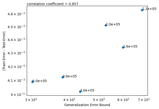
(a) $\delta$=$0.25$, correlation = $0.857$

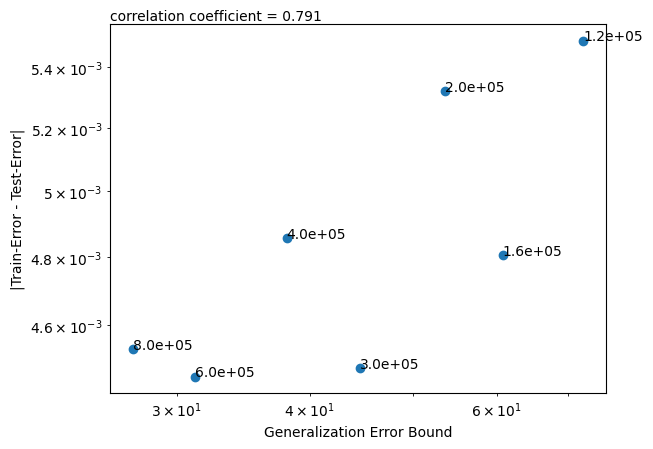
(b) $\delta$=$0.4$, correlation = $0.791$

Figure 2: The above plot shows the behaviour of the measured generalization error with respect to $\frac{\mathcal{C}_{3,2}\,\tilde{\mathcal{C}}_{-2,-2}}{\sqrt{m}}$ for training DeepONets with empirical loss as given in equation 11, specialized to the Huber loss (Definition 6) for the stated values of $\delta$ and for the branch and the trunk nets being of depth $3$. Each point is labelled by the number of training data used in that experiment.

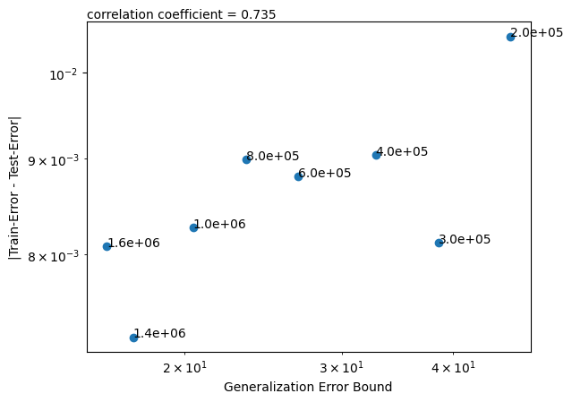
Figure 3: The above plot shows the behaviour of the measured generalization error with respect to $\frac{\mathcal{C}_{3,2}\,\tilde{\mathcal{C}}_{-2,-2}}{\sqrt{m}}$ for training DeepONets with empirical loss as given in equation 11, specialized to the $\ell_{2}$ loss and for the branch and the trunk nets being of depth $3$. Each point is labelled by the number of training data used in that experiment.

3 Discussion

The most immediate research direction that is being suggested by our generalization error bound is to explore if the advantages shown here for Huber loss can make DeepONets competitive with CNO [mishra2023convolutional].

Further, in [pidon], an unsupervised variation of the loss function of a DeepONet was shown to give better performance. In [vdon], authors employ a variational framework for solving differential equations using DeepONets, through a novel loss function. Understanding precisely when these variations in the loss function used give advantages over the basic DeepONet loss is yet another interesting direction for future research - and the path towards such goals could be to explore if the methods demonstrated here for computation of generalization bounds can be used for these novel setups too.

Also, it would be fruitful to understand how the generalization bounds obtained in this work can be modified to cater to the variations of the DeepONet architecture [kontolati2023learning], [bonev2023spherical] [lu_fair] that are getting deployed.

In the context of understanding the generalization error of Siamese networks, the authors in [puruxml] dealt with a certain product of neural outputs structure (where the nets share weights). In their analysis, the authors bound the Rademacher complexity via covering numbers. Since we try to directly bound the Rademacher complexity for DeepONets, it would be interesting to investigate if our methods can be adapted to improve such results about Siamese nets.

Lastly, we note that the existing bounds on the Rademacher complexity of nets have typically been proven by making ingenious use of the algebraic identities satisfied by Rademacher complexity (Theorem $12$ in [bartlett]). But to the best of our knowledge, we are not aware of any general result on how Rademacher complexity of a product of function spaces can be written in terms of individual Rademacher complexities. We posit that such a mathematical development, if achieved in generality, can be a significant advance affecting various fields.

4 Methods

In this section, we will outline the proofs of the main results, Theorems 1 and 2. We would like to emphasize that the subsequent propositions 3 and 4 hold in more generality than Theorem 1, because they do not need the branch and the trunk nets to be of equal depth.

Outline of the Proof Techniques

Derivation of the first main result, Theorem 1, involves $3$ key steps:  (a) formulating a variation of the standard Talagrand contraction (Lemma 1)  (b) using this to bound the Rademacher complexity of a class of DeepONets with certain activations (e.g. absolute value) by the Rademacher complexity for a class of DeepONets having one less depth and $1-$dimensional outputs, for both the branch and the trunk (Lemma 3) and lastly  (c) uncovering a recursive structure for the Rademacher complexity across depths between special DeepONet classes having $1-$dimensional outputs for both the branch and the trunk. (Lemma 4).

Lemma 3 removes the last $4$ matrices from the DeepONet ($2$ each from the branch and the trunk) leading to one-dimensional output branch and trunk nets. Lemma 4 removes 2 matrices ($1$ each from branch and trunk) – by an entirely different argument than needed in the former. Lemma 3 is invoked only once at the beginning, while Lemma 4 is repeatedly used for each remaining layer of the DeepONet.

We note that both our “peeling” lemmas above are structurally very different from the one in [rgs] - where the last layer of a standard net gets peeled in every step.

Deriving the second main result, Theorem 2, involves the following key steps:  (a) establishing a relationship between the Rademacher complexity of the loss class and that of the ${\rm DeepONet}$ when the loss function is Lipschitz (Proposition LABEL:thm:gen) and (b) using this to upper bound the expectation over data of the supremum of generalization error in terms of the Rademacher complexity of the DeepONet.

Towards proving Theorem 1, we need the following lemma which can be seen as a variation of the standard Talagrand contraction lemma,

Lemma 1

Let $\phi_{P},\phi_{Q}:\mathbb{R}\rightarrow\mathbb{R}$ be two functions such that Assumption 5 holds and let $\cal{P}$ and $\cal{Q}$ be any two sets of real-valued functions. Then given any two sets of points $\{{\mathchoice{\mbox{\boldmath$\displaystyle\bf x$}}{\mbox{\boldmath$\textstyle\bf x$}}{\mbox{\boldmath$\scriptstyle\bf x$}}{\mbox{\boldmath$\scriptscriptstyle\bf x$}}}_{i}\mid i=1,\ldots,m\}$ and $\{{\mathchoice{\mbox{\boldmath$\displaystyle\bf y$}}{\mbox{\boldmath$\textstyle\bf y$}}{\mbox{\boldmath$\scriptstyle\bf y$}}{\mbox{\boldmath$\scriptscriptstyle\bf y$}}}_{i}\mid i=1,\ldots,m\}$ in the domains of the functions in $\cal P$ and $\cal Q$ respectively, we have the following inequality of Rademacher complexities - where both the sides are being evaluated on this same set of points,

$${\bf\mathcal{R}}_{\rm m}(\phi_{P}\circ\mathcal{P}\cdot\phi_{Q}\circ\mathcal{Q})\leq L{\bf\mathcal{R}}_{\rm m}(\cal{P}\cdot\cal Q).$$

The above lemma has been proven in Appendix LABEL:proof:contraction1.

Towards stating Propositions 3 and 4, we will need to define a class of sub-DeepONets s.t these sub-DeepONets would be one depth lower in the branch and trunk network, and would always have one dimensional outputs for both the branch and trunk nets and would share weights below that with the corresponding layers in the original DeepONet.

Definition 2

(Classes of sub-DeepONets)

• Let ${\bf\mathcal{W}}_{\rm rest}$ be a set of allowed matrices for nets $f^{\prime}_{B}$ and $f^{\prime}_{T}$ as in Definition 4.

• Further, given a constant $\mathcal{C}_{q_{B},q_{T},q_{B}-1,q_{T}-1}>0$ we define the following set of $4-$tuples of outermost layer of matrices in the ${\rm DeepONet}$ as,

  $${\bf\mathcal{W}}(\mathcal{C}_{q_{B},q_{T},q_{B}-1,q_{T}-1})\coloneqq\Bigg{\{}(\mathbf{B}_{q_{B}},\mathbf{B}_{q_{B}-1},\mathbf{T}_{q_{T}},\mathbf{T}_{q_{T}-1})\,\,\Bigg{|}$$

  $$\sum_{k_{1}=1}^{b_{-1}}\sum_{k_{2}=1}^{t_{-1}}\norm{\mathbf{B}_{q_{B}-1,k_{1}}}\cdot\norm{\mathbf{T}_{q_{T}-1,k_{2}}}\cdot\absolutevalue{\Big{[}\sum_{j=1}^{p}(\mathbf{B}_{q_{B},j}\mathbf{T}_{q_{T},j}^{\top})\Big{]}_{k_{1},k_{2}}}\leq\mathcal{C}_{q_{B},q_{T},q_{B}-1,q_{T}-1}\Bigg{\}}.$$ (12)

• Corresponding to the above we define the following class of ${\rm DeepONet}$s,

  $${\rm DeepONet}({\bf\mathcal{W}}(\mathcal{C}_{q_{B},q_{T},q_{B}-1,q_{T}-1}),{\bf\mathcal{W}}_{\rm rest}) \coloneqq$$

  $$\Big{\{}{\rm DeepONet}_{\mathchoice{\mbox{\boldmath$\displaystyle\bf w$}}{\mbox{\boldmath$\textstyle\bf w$}}{\mbox{\boldmath$\scriptstyle\bf w$}}{\mbox{\boldmath$\scriptscriptstyle\bf w$}}}\text{ (as in Definition \ref{def:doneq})}\,\, \Big{|}\,\,{\mathchoice{\mbox{\boldmath$\displaystyle\bf w$}}{\mbox{\boldmath$\textstyle\bf w$}}{\mbox{\boldmath$\scriptstyle\bf w$}}{\mbox{\boldmath$\scriptscriptstyle\bf w$}}}\in({\bf\mathcal{W}}(\mathcal{C}_{q_{B},q_{T},q_{B}-1,q_{T}-1}),{\bf\mathcal{W}}_{\rm rest})\Big{\}}.$$ (13)

• Lastly, we define the following class of DeepONets,

  $${\rm DeepONet}({\bf\mathcal{W}}_{\rm rest})\coloneqq\Bigg{\{}({\mathchoice{\mbox{\boldmath$\displaystyle\bf x$}}{\mbox{\boldmath$\textstyle\bf x$}}{\mbox{\boldmath$\scriptstyle\bf x$}}{\mbox{\boldmath$\scriptscriptstyle\bf x$}}}_{B},{\mathchoice{\mbox{\boldmath$\displaystyle\bf x$}}{\mbox{\boldmath$\textstyle\bf x$}}{\mbox{\boldmath$\scriptstyle\bf x$}}{\mbox{\boldmath$\scriptscriptstyle\bf x$}}}_{T})\mapsto{\mathchoice{\mbox{\boldmath$\displaystyle\bf v$}}{\mbox{\boldmath$\textstyle\bf v$}}{\mbox{\boldmath$\scriptstyle\bf v$}}{\mbox{\boldmath$\scriptscriptstyle\bf v$}}}^{\top}{\mathchoice{\mbox{\boldmath$\displaystyle\bf f$}}{\mbox{\boldmath$\textstyle\bf f$}}{\mbox{\boldmath$\scriptstyle\bf f$}}{\mbox{\boldmath$\scriptscriptstyle\bf f$}}}^{\prime}_{B}({\mathchoice{\mbox{\boldmath$\displaystyle\bf x$}}{\mbox{\boldmath$\textstyle\bf x$}}{\mbox{\boldmath$\scriptstyle\bf x$}}{\mbox{\boldmath$\scriptscriptstyle\bf x$}}}_{B})\cdot{\mathchoice{\mbox{\boldmath$\displaystyle\bf w$}}{\mbox{\boldmath$\textstyle\bf w$}}{\mbox{\boldmath$\scriptstyle\bf w$}}{\mbox{\boldmath$\scriptscriptstyle\bf w$}}}^{\top}{\mathchoice{\mbox{\boldmath$\displaystyle\bf f$}}{\mbox{\boldmath$\textstyle\bf f$}}{\mbox{\boldmath$\scriptstyle\bf f$}}{\mbox{\boldmath$\scriptscriptstyle\bf f$}}}^{\prime}_{T}({\mathchoice{\mbox{\boldmath$\displaystyle\bf x$}}{\mbox{\boldmath$\textstyle\bf x$}}{\mbox{\boldmath$\scriptstyle\bf x$}}{\mbox{\boldmath$\scriptscriptstyle\bf x$}}}_{T})\in\mathbb{R}$$ (14)

  $$\bigg{|}\,\,\,\text{the set of allowed matrices for nets }\leavevmode\nobreak\ f^{\prime}_{B}\leavevmode\nobreak\ \&\leavevmode\nobreak\ f^{\prime}_{T}\text{ are in }{\bf\mathcal{W}}_{\rm rest}\,\,;\,\,\leavevmode\nobreak\ ({\mathchoice{\mbox{\boldmath$\displaystyle\bf v$}}{\mbox{\boldmath$\textstyle\bf v$}}{\mbox{\boldmath$\scriptstyle\bf v$}}{\mbox{\boldmath$\scriptscriptstyle\bf v$}}},{\mathchoice{\mbox{\boldmath$\displaystyle\bf w$}}{\mbox{\boldmath$\textstyle\bf w$}}{\mbox{\boldmath$\scriptstyle\bf w$}}{\mbox{\boldmath$\scriptscriptstyle\bf w$}}})\in S^{b_{-2}-1}\times S^{t_{-2}-1}\,\Bigg{\}}.$$

Proposition 3 (Removal of the Last $4$ Matrices of a DeepONet)

We continue to be in the setup of Definition 4 and assuming that $\sigma_{1},\sigma_{2}$ satisfies Assumption 5 for some $L>0$, and are positively homogeneous. Then given the definitions of ${\rm DeepONet}({\bf\mathcal{W}}(\mathcal{C}_{q_{B},q_{T},q_{B}-1,q_{T}-1}),{\bf\mathcal{W}}_{\rm rest})$ and ${\rm DeepONet}({\bf\mathcal{W}}_{\rm rest})$ in Definition 2, we have the following upperbound on empirical Rademacher complexity of a DeepONet, (here ${\bf\mathcal{S}}_{k}\coloneqq S^{b_{-k}-1}\times S^{t_{-k}-1}$)

$$\hat{\mathcal{R}}_{m}\Big{(}{\rm DeepONet}({\bf\mathcal{W}}(\mathcal{C}_{q_{B},q_{T},q_{B}-1,q_{T}-1}),{\bf\mathcal{W}}_{\rm rest})\Big{)}$$

$$\leq 2L\cdot\mathcal{C}_{q_{B},q_{T},q_{B}-1,q_{T}-1}\cdot\mathbb{E}_{\epsilon}\Bigg{[}\sup_{\begin{subarray}{c}({\mathchoice{\mbox{\boldmath$\displaystyle\bf v$}}{\mbox{\boldmath$\textstyle\bf v$}}{\mbox{\boldmath$\scriptstyle\bf v$}}{\mbox{\boldmath$\scriptscriptstyle\bf v$}}},{\mathchoice{\mbox{\boldmath$\displaystyle\bf w$}}{\mbox{\boldmath$\textstyle\bf w$}}{\mbox{\boldmath$\scriptstyle\bf w$}}{\mbox{\boldmath$\scriptscriptstyle\bf w$}}})\,\in\,{\bf\mathcal{S}}_{2}\\ {\bf\mathcal{W}}_{\rm rest}\end{subarray}}\Bigg{(}\sum_{i=1}^{m}\epsilon_{i}{\mathchoice{\mbox{\boldmath$\displaystyle\bf v$}}{\mbox{\boldmath$\textstyle\bf v$}}{\mbox{\boldmath$\scriptstyle\bf v$}}{\mbox{\boldmath$\scriptscriptstyle\bf v$}}}^{\top}{\mathchoice{\mbox{\boldmath$\displaystyle\bf f$}}{\mbox{\boldmath$\textstyle\bf f$}}{\mbox{\boldmath$\scriptstyle\bf f$}}{\mbox{\boldmath$\scriptscriptstyle\bf f$}}}^{\prime}_{B}({\mathchoice{\mbox{\boldmath$\displaystyle\bf x$}}{\mbox{\boldmath$\textstyle\bf x$}}{\mbox{\boldmath$\scriptstyle\bf x$}}{\mbox{\boldmath$\scriptscriptstyle\bf x$}}}_{B,i})\cdot{\mathchoice{\mbox{\boldmath$\displaystyle\bf w$}}{\mbox{\boldmath$\textstyle\bf w$}}{\mbox{\boldmath$\scriptstyle\bf w$}}{\mbox{\boldmath$\scriptscriptstyle\bf w$}}}^{\top}{\mathchoice{\mbox{\boldmath$\displaystyle\bf f$}}{\mbox{\boldmath$\textstyle\bf f$}}{\mbox{\boldmath$\scriptstyle\bf f$}}{\mbox{\boldmath$\scriptscriptstyle\bf f$}}}^{\prime}_{T}({\mathchoice{\mbox{\boldmath$\displaystyle\bf x$}}{\mbox{\boldmath$\textstyle\bf x$}}{\mbox{\boldmath$\scriptstyle\bf x$}}{\mbox{\boldmath$\scriptscriptstyle\bf x$}}}_{T,i})\Bigg{)}\Bigg{]}$$

$$\leq 2L\cdot\mathcal{C}_{q_{B},q_{T},q_{B}-1,q_{T}-1}\cdot\hat{\mathcal{R}}_{m}\Big{(}{\rm DeepONet}({\bf\mathcal{W}}_{\rm rest})\Big{)}.$$

Note that both sides of the above are computed for the same data $\{({\mathchoice{\mbox{\boldmath$\displaystyle\bf x$}}{\mbox{\boldmath$\textstyle\bf x$}}{\mbox{\boldmath$\scriptstyle\bf x$}}{\mbox{\boldmath$\scriptscriptstyle\bf x$}}}_{B,i},{\mathchoice{\mbox{\boldmath$\displaystyle\bf x$}}{\mbox{\boldmath$\textstyle\bf x$}}{\mbox{\boldmath$\scriptstyle\bf x$}}{\mbox{\boldmath$\scriptscriptstyle\bf x$}}}_{T,i})\in\mathbb{R}^{d_{1}}\times\mathbb{R}^{d_{2}}\mid i=1,\ldots,m\}$. The proof of the above proposition is given in Appendix LABEL:outerpeelproof.

Referring to the definitions of the ${\rm DeepONet}$ classes on the L.H.S. and the R.H.S. of the above, as given in equations • ‣ 2 and 14 respectively, we see that the above lemma upperbounds the Rademacher complexity of a ${\rm DeepONet}$ class (whose individual nets can have multi-dimensional outputs) by the Rademacher complexity of a simpler ${\rm DeepONet}$ class. The ${\rm DeepONet}$ class in the R.H.S. is simpler because the last layer of each of the individual nets therein is constrained to be a unit vector of appropriate dimensions (and thus the individual nets here are always of $1$ dimensional output) – and whose both branch and the trunk are shorter in depth by $1$ activation and $1$ linear transform than in the L.H.S.

Proposition 4 (Peeling for DeepONets)

We continue in the setup of Proposition 3 and define the functions ${\mathchoice{\mbox{\boldmath$\displaystyle\bf f$}}{\mbox{\boldmath$\textstyle\bf f$}}{\mbox{\boldmath$\scriptstyle\bf f$}}{\mbox{\boldmath$\scriptscriptstyle\bf f$}}}^{\prime\prime}_{B}$ and ${\mathchoice{\mbox{\boldmath$\displaystyle\bf f$}}{\mbox{\boldmath$\textstyle\bf f$}}{\mbox{\boldmath$\scriptstyle\bf f$}}{\mbox{\boldmath$\scriptscriptstyle\bf f$}}}^{\prime\prime}_{T}$ s.t we have the following equalities, ${\mathchoice{\mbox{\boldmath$\displaystyle\bf f$}}{\mbox{\boldmath$\textstyle\bf f$}}{\mbox{\boldmath$\scriptstyle\bf f$}}{\mbox{\boldmath$\scriptscriptstyle\bf f$}}}^{\prime}_{B}=\sigma_{1}\left(\mathbf{B}_{q_{B}-2}{\mathchoice{\mbox{\boldmath$\displaystyle\bf f$}}{\mbox{\boldmath$\textstyle\bf f$}}{\mbox{\boldmath$\scriptstyle\bf f$}}{\mbox{\boldmath$\scriptscriptstyle\bf f$}}}^{\prime\prime}_{B}\right)\leavevmode\nobreak\ \&{\mathchoice{\mbox{\boldmath$\displaystyle\bf f$}}{\mbox{\boldmath$\textstyle\bf f$}}{\mbox{\boldmath$\scriptstyle\bf f$}}{\mbox{\boldmath$\scriptscriptstyle\bf f$}}}^{\prime}_{T}=\sigma_{2}\left(\mathbf{T}_{q_{T}-2}{\mathchoice{\mbox{\boldmath$\displaystyle\bf f$}}{\mbox{\boldmath$\textstyle\bf f$}}{\mbox{\boldmath$\scriptstyle\bf f$}}{\mbox{\boldmath$\scriptscriptstyle\bf f$}}}^{\prime\prime}_{T}\right)$ Further, given a constant $\mathcal{C}_{-2,-2}>0$, we define ${\bf\mathcal{W}}^{\prime}_{rest}$ as the union of (a) the set of weights that are allowed in the ${\bf\mathcal{W}}_{rest}$ set for the matrices $\mathbf{B}_{q_{B}-3},\mathbf{B}_{q_{B}-4},\ldots,\mathbf{B}_{1}$ and $\mathbf{T}_{q_{T}-3},\mathbf{T}_{q_{T}-4},\ldots,\mathbf{T}_{1}$ and (b) the subset of the weights for $\mathbf{B}_{q_{B}-2}\leavevmode\nobreak\ \&\leavevmode\nobreak\ \mathbf{T}_{q_{T}-2}$ that are allowed by ${\bf\mathcal{W}}_{rest}$ which also additionally satisfy the constraint, (here ${\bf\mathcal{S}}_{k}\coloneqq S^{b_{-k}-1}\times S^{t_{-k}-1}$)

$$\sup_{\begin{subarray}{c}({\mathchoice{\mbox{\boldmath$\displaystyle\bf v$}}{\mbox{\boldmath$\textstyle\bf v$}}{\mbox{\boldmath$\scriptstyle\bf v$}}{\mbox{\boldmath$\scriptscriptstyle\bf v$}}},{\mathchoice{\mbox{\boldmath$\displaystyle\bf w$}}{\mbox{\boldmath$\textstyle\bf w$}}{\mbox{\boldmath$\scriptstyle\bf w$}}{\mbox{\boldmath$\scriptscriptstyle\bf w$}}})\,\in\,{\bf\mathcal{S}}_{2}\end{subarray}}\sum_{j_{1}=1}^{b_{-2}}\sum_{j_{2}=1}^{t_{-2}}\absolutevalue{({\mathchoice{\mbox{\boldmath$\displaystyle\bf v$}}{\mbox{\boldmath$\textstyle\bf v$}}{\mbox{\boldmath$\scriptstyle\bf v$}}{\mbox{\boldmath$\scriptscriptstyle\bf v$}}}{\mathchoice{\mbox{\boldmath$\displaystyle\bf w$}}{\mbox{\boldmath$\textstyle\bf w$}}{\mbox{\boldmath$\scriptstyle\bf w$}}{\mbox{\boldmath$\scriptscriptstyle\bf w$}}}^{\top})_{j_{1},j_{2}}}\norm{\mathbf{B}_{q_{B}-2,j_{1}}}\norm{\mathbf{T}_{q_{T}-2,j_{2}}}\leq\mathcal{C}_{-2,-2}.$$ (15)

Then we get the following inequality between Rademacher complexities,

$$\mathbb{E}_{\epsilon}\Bigg{[}\sup_{\begin{subarray}{c}({\mathchoice{\mbox{\boldmath$\displaystyle\bf v$}}{\mbox{\boldmath$\textstyle\bf v$}}{\mbox{\boldmath$\scriptstyle\bf v$}}{\mbox{\boldmath$\scriptscriptstyle\bf v$}}},{\mathchoice{\mbox{\boldmath$\displaystyle\bf w$}}{\mbox{\boldmath$\textstyle\bf w$}}{\mbox{\boldmath$\scriptstyle\bf w$}}{\mbox{\boldmath$\scriptscriptstyle\bf w$}}})\,\in\,{\bf\mathcal{S}}_{2}\\ {\bf\mathcal{W}}_{\rm rest}\end{subarray}}\Bigg{(}\sum_{i=1}^{m}\epsilon_{i}{\mathchoice{\mbox{\boldmath$\displaystyle\bf v$}}{\mbox{\boldmath$\textstyle\bf v$}}{\mbox{\boldmath$\scriptstyle\bf v$}}{\mbox{\boldmath$\scriptscriptstyle\bf v$}}}^{\top}{\mathchoice{\mbox{\boldmath$\displaystyle\bf f$}}{\mbox{\boldmath$\textstyle\bf f$}}{\mbox{\boldmath$\scriptstyle\bf f$}}{\mbox{\boldmath$\scriptscriptstyle\bf f$}}}^{\prime}_{B}({\mathchoice{\mbox{\boldmath$\displaystyle\bf x$}}{\mbox{\boldmath$\textstyle\bf x$}}{\mbox{\boldmath$\scriptstyle\bf x$}}{\mbox{\boldmath$\scriptscriptstyle\bf x$}}}_{B,i})\cdot{\mathchoice{\mbox{\boldmath$\displaystyle\bf w$}}{\mbox{\boldmath$\textstyle\bf w$}}{\mbox{\boldmath$\scriptstyle\bf w$}}{\mbox{\boldmath$\scriptscriptstyle\bf w$}}}^{\top}{\mathchoice{\mbox{\boldmath$\displaystyle\bf f$}}{\mbox{\boldmath$\textstyle\bf f$}}{\mbox{\boldmath$\scriptstyle\bf f$}}{\mbox{\boldmath$\scriptscriptstyle\bf f$}}}^{\prime}_{T}({\mathchoice{\mbox{\boldmath$\displaystyle\bf x$}}{\mbox{\boldmath$\textstyle\bf x$}}{\mbox{\boldmath$\scriptstyle\bf x$}}{\mbox{\boldmath$\scriptscriptstyle\bf x$}}}_{T,i})\Bigg{)}\Bigg{]}$$

$$\leq 2L\mathcal{C}_{-2,-2}\mathbb{E}_{\epsilon}\Bigg{[}\sup_{\begin{subarray}{c}({\mathchoice{\mbox{\boldmath$\displaystyle\bf v$}}{\mbox{\boldmath$\textstyle\bf v$}}{\mbox{\boldmath$\scriptstyle\bf v$}}{\mbox{\boldmath$\scriptscriptstyle\bf v$}}},{\mathchoice{\mbox{\boldmath$\displaystyle\bf w$}}{\mbox{\boldmath$\textstyle\bf w$}}{\mbox{\boldmath$\scriptstyle\bf w$}}{\mbox{\boldmath$\scriptscriptstyle\bf w$}}})\,\in\,{\bf\mathcal{S}}_{3}\\ {\bf\mathcal{W}}^{\prime}_{rest}\end{subarray}}\left({\sum_{i=1}^{m}\epsilon_{i}({\mathchoice{\mbox{\boldmath$\displaystyle\bf v$}}{\mbox{\boldmath$\textstyle\bf v$}}{\mbox{\boldmath$\scriptstyle\bf v$}}{\mbox{\boldmath$\scriptscriptstyle\bf v$}}}^{\top}{\mathchoice{\mbox{\boldmath$\displaystyle\bf f$}}{\mbox{\boldmath$\textstyle\bf f$}}{\mbox{\boldmath$\scriptstyle\bf f$}}{\mbox{\boldmath$\scriptscriptstyle\bf f$}}}^{\prime\prime}_{B}({\mathchoice{\mbox{\boldmath$\displaystyle\bf x$}}{\mbox{\boldmath$\textstyle\bf x$}}{\mbox{\boldmath$\scriptstyle\bf x$}}{\mbox{\boldmath$\scriptscriptstyle\bf x$}}}_{B,i}))({\mathchoice{\mbox{\boldmath$\displaystyle\bf w$}}{\mbox{\boldmath$\textstyle\bf w$}}{\mbox{\boldmath$\scriptstyle\bf w$}}{\mbox{\boldmath$\scriptscriptstyle\bf w$}}}^{\top}{\mathchoice{\mbox{\boldmath$\displaystyle\bf f$}}{\mbox{\boldmath$\textstyle\bf f$}}{\mbox{\boldmath$\scriptstyle\bf f$}}{\mbox{\boldmath$\scriptscriptstyle\bf f$}}}_{T}^{\prime\prime}({\mathchoice{\mbox{\boldmath$\displaystyle\bf x$}}{\mbox{\boldmath$\textstyle\bf x$}}{\mbox{\boldmath$\scriptstyle\bf x$}}{\mbox{\boldmath$\scriptscriptstyle\bf x$}}}_{T,i}))}\right)\Bigg{]},$$

where $b_{-k},t_{-k}$ are as in Definition 4.

Proof of the above proposition is given in Appendix LABEL:proof:peel. And now we have stated all the intermediate results needed to prove our bounds on the Rademacher complexity of a certain DeepONet class.

Proof of Theorem 1

Proof  [] For each $k=2,3,\ldots,n-1,\,$ we define a product of unit-spheres, $\mathcal{S}_{k}:=S^{b_{-k}-1}\times S^{t_{-k}-1}$ and let $\mathcal{S}_{n}\coloneqq S^{d_{1}-1}\times S^{d_{2}-1}.$ Now we define,

$${\bf\mathcal{W}}_{\rm rest}^{1}\coloneqq\bigg{\{}(\mathbf{B}_{n},\mathbf{B}_{n-1},\mathbf{T}_{n},\mathbf{T}_{n-1})\,\,\bigg{\mid}\,\,\sum_{k_{1}=1}^{b_{-1}}\sum_{k_{2}=1}^{t_{-1}}\norm{\mathbf{B}_{n-1,k_{1}}}\cdot\norm{\mathbf{T}_{n-1,k_{2}}}\cdot\bigg{[}\sum_{j=1}^{p}(\mathbf{B}_{n,j}\mathbf{T}_{n,j}^{\top})\bigg{]}_{k_{1},k_{2}}\leq\mathcal{C}_{n,n-1}\bigg{\}}.$$

Next, for each $i=2,3,\ldots,n-1$, we define

$${\bf\mathcal{W}}_{\rm rest}^{i}\coloneqq\bigcup_{k=1}^{n-i}\bigg{\{}(\mathbf{B}_{k},\mathbf{T}_{k})\,\,\bigg{\mid}\,\,\sup_{\begin{subarray}{c}({\mathchoice{\mbox{\boldmath$\displaystyle\bf v$}}{\mbox{\boldmath$\textstyle\bf v$}}{\mbox{\boldmath$\scriptstyle\bf v$}}{\mbox{\boldmath$\scriptscriptstyle\bf v$}}},{\mathchoice{\mbox{\boldmath$\displaystyle\bf w$}}{\mbox{\boldmath$\textstyle\bf w$}}{\mbox{\boldmath$\scriptstyle\bf w$}}{\mbox{\boldmath$\scriptscriptstyle\bf w$}}})\,\in\,{\bf\mathcal{S}}_{k}\end{subarray}}\sum_{j_{1}=1}^{b_{-k}}\sum_{j_{2}=1}^{t_{-k}}\absolutevalue{({\mathchoice{\mbox{\boldmath$\displaystyle\bf v$}}{\mbox{\boldmath$\textstyle\bf v$}}{\mbox{\boldmath$\scriptstyle\bf v$}}{\mbox{\boldmath$\scriptscriptstyle\bf v$}}}{\mathchoice{\mbox{\boldmath$\displaystyle\bf w$}}{\mbox{\boldmath$\textstyle\bf w$}}{\mbox{\boldmath$\scriptstyle\bf w$}}{\mbox{\boldmath$\scriptscriptstyle\bf w$}}}^{\top})_{j_{1},j_{2}}}\cdot\norm{\mathbf{B}_{n-k,j_{1}}}\cdot\norm{\mathbf{T}_{n-k,j_{2}}}\leq\mathcal{C}_{-k,-k}\bigg{\}}.$$

Thus we have,

$$m\hat{\mathcal{R}}_{m}=\mathbb{E}_{\epsilon}\Bigg{[}\sup_{\begin{subarray}{c}({\bf\mathcal{W}}_{\rm rest}^{1},{\bf\mathcal{W}}_{\rm rest}^{2})\end{subarray}}\left(\sum_{i=1}^{m}\epsilon_{i}\left\langle\mathbf{B}_{n}\sigma_{1}\left(\mathbf{B}_{n-1}{\mathchoice{\mbox{\boldmath$\displaystyle\bf f$}}{\mbox{\boldmath$\textstyle\bf f$}}{\mbox{\boldmath$\scriptstyle\bf f$}}{\mbox{\boldmath$\scriptscriptstyle\bf f$}}}^{\prime}_{B}({\mathchoice{\mbox{\boldmath$\displaystyle\bf x$}}{\mbox{\boldmath$\textstyle\bf x$}}{\mbox{\boldmath$\scriptstyle\bf x$}}{\mbox{\boldmath$\scriptscriptstyle\bf x$}}}_{B,i})\right),\mathbf{T}_{n}\sigma_{2}\left(\mathbf{T}_{n-1}{\mathchoice{\mbox{\boldmath$\displaystyle\bf f$}}{\mbox{\boldmath$\textstyle\bf f$}}{\mbox{\boldmath$\scriptstyle\bf f$}}{\mbox{\boldmath$\scriptscriptstyle\bf f$}}}^{\prime}_{T}({\mathchoice{\mbox{\boldmath$\displaystyle\bf x$}}{\mbox{\boldmath$\textstyle\bf x$}}{\mbox{\boldmath$\scriptstyle\bf x$}}{\mbox{\boldmath$\scriptscriptstyle\bf x$}}}_{T,i})\right)\right\rangle\right)\Bigg{]}.$$

Then we can invoke Lemma 3 on the above to get,

$$m\hat{\mathcal{R}}_{m} =\mathbb{E}_{\epsilon}\Bigg{[}\sup_{\begin{subarray}{c}({\bf\mathcal{W}}_{\rm rest}^{1},{\bf\mathcal{W}}_{\rm rest}^{2})\end{subarray}}\left(\sum_{i=1}^{m}\epsilon_{i}\left\langle\mathbf{B}_{n}\sigma_{1}\left(\mathbf{B}_{n-1}{\mathchoice{\mbox{\boldmath$\displaystyle\bf f$}}{\mbox{\boldmath$\textstyle\bf f$}}{\mbox{\boldmath$\scriptstyle\bf f$}}{\mbox{\boldmath$\scriptscriptstyle\bf f$}}}^{\prime}_{B}({\mathchoice{\mbox{\boldmath$\displaystyle\bf x$}}{\mbox{\boldmath$\textstyle\bf x$}}{\mbox{\boldmath$\scriptstyle\bf x$}}{\mbox{\boldmath$\scriptscriptstyle\bf x$}}}_{B,i})\right),\mathbf{T}_{n}\sigma_{2}\left(\mathbf{T}_{n-1}{\mathchoice{\mbox{\boldmath$\displaystyle\bf f$}}{\mbox{\boldmath$\textstyle\bf f$}}{\mbox{\boldmath$\scriptstyle\bf f$}}{\mbox{\boldmath$\scriptscriptstyle\bf f$}}}^{\prime}_{T}({\mathchoice{\mbox{\boldmath$\displaystyle\bf x$}}{\mbox{\boldmath$\textstyle\bf x$}}{\mbox{\boldmath$\scriptstyle\bf x$}}{\mbox{\boldmath$\scriptscriptstyle\bf x$}}}_{T,i})\right)\right\rangle\right)\Bigg{]}$$

$$\leq 2L\mathcal{C}_{n,n-1}\mathbb{E}_{\epsilon}\Bigg{[}\sup_{\begin{subarray}{c}{\bf\mathcal{W}}_{\rm rest}^{2}\\ {\mathchoice{\mbox{\boldmath$\displaystyle\bf v$}}{\mbox{\boldmath$\textstyle\bf v$}}{\mbox{\boldmath$\scriptstyle\bf v$}}{\mbox{\boldmath$\scriptscriptstyle\bf v$}}}_{1},{\mathchoice{\mbox{\boldmath$\displaystyle\bf v$}}{\mbox{\boldmath$\textstyle\bf v$}}{\mbox{\boldmath$\scriptstyle\bf v$}}{\mbox{\boldmath$\scriptscriptstyle\bf v$}}}_{2}\,\in\,\mathcal{S}_{2}\end{subarray}}\left(\sum_{i=1}^{m}\epsilon_{i}{{\mathchoice{\mbox{\boldmath$\displaystyle\bf v$}}{\mbox{\boldmath$\textstyle\bf v$}}{\mbox{\boldmath$\scriptstyle\bf v$}}{\mbox{\boldmath$\scriptscriptstyle\bf v$}}}_{1}^{\top}{\mathchoice{\mbox{\boldmath$\displaystyle\bf f$}}{\mbox{\boldmath$\textstyle\bf f$}}{\mbox{\boldmath$\scriptstyle\bf f$}}{\mbox{\boldmath$\scriptscriptstyle\bf f$}}}^{\prime}_{B}({\mathchoice{\mbox{\boldmath$\displaystyle\bf x$}}{\mbox{\boldmath$\textstyle\bf x$}}{\mbox{\boldmath$\scriptstyle\bf x$}}{\mbox{\boldmath$\scriptscriptstyle\bf x$}}}_{B,i})}\,{{\mathchoice{\mbox{\boldmath$\displaystyle\bf v$}}{\mbox{\boldmath$\textstyle\bf v$}}{\mbox{\boldmath$\scriptstyle\bf v$}}{\mbox{\boldmath$\scriptscriptstyle\bf v$}}}_{2}^{\top}{\mathchoice{\mbox{\boldmath$\displaystyle\bf f$}}{\mbox{\boldmath$\textstyle\bf f$}}{\mbox{\boldmath$\scriptstyle\bf f$}}{\mbox{\boldmath$\scriptscriptstyle\bf f$}}}^{\prime}_{T}({\mathchoice{\mbox{\boldmath$\displaystyle\bf x$}}{\mbox{\boldmath$\textstyle\bf x$}}{\mbox{\boldmath$\scriptstyle\bf x$}}{\mbox{\boldmath$\scriptscriptstyle\bf x$}}}_{T,i})}\right)\Bigg{]}.$$

Now, using Lemma 4 repeatedly on the R.H.S above, and defining in a natural fashion the subsequent branch and trunk sub-networks as ${\mathchoice{\mbox{\boldmath$\displaystyle\bf f$}}{\mbox{\boldmath$\textstyle\bf f$}}{\mbox{\boldmath$\scriptstyle\bf f$}}{\mbox{\boldmath$\scriptscriptstyle\bf f$}}}^{(i)}(\cdot)$ we have,

$$m\hat{\mathcal{R}}_{m} \leq(2L)^{2}\mathcal{C}_{n,n-1}\,\mathcal{C}_{-2,-2}\mathbb{E}_{\epsilon}\left(\sup_{\begin{subarray}{c}{\bf\mathcal{W}}_{rest}^{3}\\ ({\mathchoice{\mbox{\boldmath$\displaystyle\bf v$}}{\mbox{\boldmath$\textstyle\bf v$}}{\mbox{\boldmath$\scriptstyle\bf v$}}{\mbox{\boldmath$\scriptscriptstyle\bf v$}}}_{1},{\mathchoice{\mbox{\boldmath$\displaystyle\bf v$}}{\mbox{\boldmath$\textstyle\bf v$}}{\mbox{\boldmath$\scriptstyle\bf v$}}{\mbox{\boldmath$\scriptscriptstyle\bf v$}}}_{2})\,\in\,{\bf\mathcal{S}}_{3}\end{subarray}}{\sum_{i=1}^{m}\epsilon_{i}({\mathchoice{\mbox{\boldmath$\displaystyle\bf v$}}{\mbox{\boldmath$\textstyle\bf v$}}{\mbox{\boldmath$\scriptstyle\bf v$}}{\mbox{\boldmath$\scriptscriptstyle\bf v$}}}_{1}^{\top}{\mathchoice{\mbox{\boldmath$\displaystyle\bf f$}}{\mbox{\boldmath$\textstyle\bf f$}}{\mbox{\boldmath$\scriptstyle\bf f$}}{\mbox{\boldmath$\scriptscriptstyle\bf f$}}}^{\prime\prime}_{B}({\mathchoice{\mbox{\boldmath$\displaystyle\bf x$}}{\mbox{\boldmath$\textstyle\bf x$}}{\mbox{\boldmath$\scriptstyle\bf x$}}{\mbox{\boldmath$\scriptscriptstyle\bf x$}}}_{B,i}))({\mathchoice{\mbox{\boldmath$\displaystyle\bf v$}}{\mbox{\boldmath$\textstyle\bf v$}}{\mbox{\boldmath$\scriptstyle\bf v$}}{\mbox{\boldmath$\scriptscriptstyle\bf v$}}}_{2}^{\top}{\mathchoice{\mbox{\boldmath$\displaystyle\bf f$}}{\mbox{\boldmath$\textstyle\bf f$}}{\mbox{\boldmath$\scriptstyle\bf f$}}{\mbox{\boldmath$\scriptscriptstyle\bf f$}}}_{T}^{\prime\prime}({\mathchoice{\mbox{\boldmath$\displaystyle\bf x$}}{\mbox{\boldmath$\textstyle\bf x$}}{\mbox{\boldmath$\scriptstyle\bf x$}}{\mbox{\boldmath$\scriptscriptstyle\bf x$}}}_{T,i}))}\right)$$

$$\mathmakebox[\widthof{{}\leq{}}][c]{\vdots}$$

$$\leq(2L)^{i}\mathcal{C}_{n,n-1}\,\left(\prod_{j=2}^{i}\mathcal{C}_{-j,-j}\right)\,\mathbb{E}_{\epsilon}\left(\sup_{\begin{subarray}{c}{\bf\mathcal{W}}_{\rm rest}^{i+1}\\ ({\mathchoice{\mbox{\boldmath$\displaystyle\bf v$}}{\mbox{\boldmath$\textstyle\bf v$}}{\mbox{\boldmath$\scriptstyle\bf v$}}{\mbox{\boldmath$\scriptscriptstyle\bf v$}}}_{1},{\mathchoice{\mbox{\boldmath$\displaystyle\bf v$}}{\mbox{\boldmath$\textstyle\bf v$}}{\mbox{\boldmath$\scriptstyle\bf v$}}{\mbox{\boldmath$\scriptscriptstyle\bf v$}}}_{2})\,\in\,{\bf\mathcal{S}}_{i+1}\end{subarray}}{\sum_{i=1}^{m}\epsilon_{i}({\mathchoice{\mbox{\boldmath$\displaystyle\bf v$}}{\mbox{\boldmath$\textstyle\bf v$}}{\mbox{\boldmath$\scriptstyle\bf v$}}{\mbox{\boldmath$\scriptscriptstyle\bf v$}}}_{1}^{\top}{\mathchoice{\mbox{\boldmath$\displaystyle\bf f$}}{\mbox{\boldmath$\textstyle\bf f$}}{\mbox{\boldmath$\scriptstyle\bf f$}}{\mbox{\boldmath$\scriptscriptstyle\bf f$}}}^{(i)}_{B}({\mathchoice{\mbox{\boldmath$\displaystyle\bf x$}}{\mbox{\boldmath$\textstyle\bf x$}}{\mbox{\boldmath$\scriptstyle\bf x$}}{\mbox{\boldmath$\scriptscriptstyle\bf x$}}}_{B,i}))({\mathchoice{\mbox{\boldmath$\displaystyle\bf v$}}{\mbox{\boldmath$\textstyle\bf v$}}{\mbox{\boldmath$\scriptstyle\bf v$}}{\mbox{\boldmath$\scriptscriptstyle\bf v$}}}_{2}^{\top}{\mathchoice{\mbox{\boldmath$\displaystyle\bf f$}}{\mbox{\boldmath$\textstyle\bf f$}}{\mbox{\boldmath$\scriptstyle\bf f$}}{\mbox{\boldmath$\scriptscriptstyle\bf f$}}}^{(i)}_{T}({\mathchoice{\mbox{\boldmath$\displaystyle\bf x$}}{\mbox{\boldmath$\textstyle\bf x$}}{\mbox{\boldmath$\scriptstyle\bf x$}}{\mbox{\boldmath$\scriptscriptstyle\bf x$}}}_{T,i}))}\right)$$

$$\mathmakebox[\widthof{{}\leq{}}][c]{\vdots}$$

$$\leq(2L)^{n-1}\mathcal{C}_{n,n-1}\,\left(\prod_{j=2}^{n-1}\mathcal{C}_{-j,-j}\right)\,\mathbb{E}_{\epsilon}\left(\sup_{\begin{subarray}{c}({\mathchoice{\mbox{\boldmath$\displaystyle\bf v$}}{\mbox{\boldmath$\textstyle\bf v$}}{\mbox{\boldmath$\scriptstyle\bf v$}}{\mbox{\boldmath$\scriptscriptstyle\bf v$}}}_{1},{\mathchoice{\mbox{\boldmath$\displaystyle\bf v$}}{\mbox{\boldmath$\textstyle\bf v$}}{\mbox{\boldmath$\scriptstyle\bf v$}}{\mbox{\boldmath$\scriptscriptstyle\bf v$}}}_{2})\,\in\,{\bf\mathcal{S}}_{n}\end{subarray}}{\sum_{i=1}^{m}\epsilon_{i}({\mathchoice{\mbox{\boldmath$\displaystyle\bf v$}}{\mbox{\boldmath$\textstyle\bf v$}}{\mbox{\boldmath$\scriptstyle\bf v$}}{\mbox{\boldmath$\scriptscriptstyle\bf v$}}}_{1}^{\top}{\mathchoice{\mbox{\boldmath$\displaystyle\bf x$}}{\mbox{\boldmath$\textstyle\bf x$}}{\mbox{\boldmath$\scriptstyle\bf x$}}{\mbox{\boldmath$\scriptscriptstyle\bf x$}}}_{B,i})({\mathchoice{\mbox{\boldmath$\displaystyle\bf v$}}{\mbox{\boldmath$\textstyle\bf v$}}{\mbox{\boldmath$\scriptstyle\bf v$}}{\mbox{\boldmath$\scriptscriptstyle\bf v$}}}_{2}^{\top}{\mathchoice{\mbox{\boldmath$\displaystyle\bf x$}}{\mbox{\boldmath$\textstyle\bf x$}}{\mbox{\boldmath$\scriptstyle\bf x$}}{\mbox{\boldmath$\scriptscriptstyle\bf x$}}}_{T,i})}\right).$$

Using Lemma 5, the final bound on the empirical Rademacher complexity becomes,

$$\hat{\mathcal{R}}_{m}\leq\frac{(2L)^{n-1}\mathcal{C}_{n,n-1}}{m}\,\left(\prod_{j=2}^{n-1}\mathcal{C}_{-j,-j}\right)\,\sqrt{\sum_{i=1}^{m}\norm{\tilde{{\mathchoice{\mbox{\boldmath$\displaystyle\bf x$}}{\mbox{\boldmath$\textstyle\bf x$}}{\mbox{\boldmath$\scriptstyle\bf x$}}{\mbox{\boldmath$\scriptscriptstyle\bf x$}}}}_{i}}_{2}^{2}}.$$

Invoking the assumption that the input is bounded s.t $\mathbb{E}\left[\norm{\tilde{{\mathchoice{\mbox{\boldmath$\displaystyle\bf x$}}{\mbox{\boldmath$\textstyle\bf x$}}{\mbox{\boldmath$\scriptstyle\bf x$}}{\mbox{\boldmath$\scriptscriptstyle\bf x$}}}}_{B}}^{2}_{2}\right]\leq M_{x,B}^{2}$ and $\mathbb{E}\left[\norm{\tilde{{\mathchoice{\mbox{\boldmath$\displaystyle\bf x$}}{\mbox{\boldmath$\textstyle\bf x$}}{\mbox{\boldmath$\scriptstyle\bf x$}}{\mbox{\boldmath$\scriptscriptstyle\bf x$}}}}_{T}}^{2}_{2}\right]\leq M_{x,T}^{2},$ the average Rademacher complexity can be bounded as

$$\mathcal{R}_{m}\leq\frac{(2L)^{n-1}\mathcal{C}_{n,n-1}}{\sqrt{m}}\,\left(\prod_{j=2}^{n-1}\mathcal{C}_{-j,-j}\right)\,{M_{x,B}M_{x,T}}.$$

$\blacksquare$

Lemma 5

$$\mathbb{E}_{\epsilon}\left(\sup_{\begin{subarray}{c}({\mathchoice{\mbox{\boldmath$\displaystyle\bf v$}}{\mbox{\boldmath$\textstyle\bf v$}}{\mbox{\boldmath$\scriptstyle\bf v$}}{\mbox{\boldmath$\scriptscriptstyle\bf v$}}}_{1},{\mathchoice{\mbox{\boldmath$\displaystyle\bf v$}}{\mbox{\boldmath$\textstyle\bf v$}}{\mbox{\boldmath$\scriptstyle\bf v$}}{\mbox{\boldmath$\scriptscriptstyle\bf v$}}}_{2})\,\in\,{\bf\mathcal{S}}_{n}\end{subarray}}{\sum_{i=1}^{m}\epsilon_{i}({\mathchoice{\mbox{\boldmath$\displaystyle\bf v$}}{\mbox{\boldmath$\textstyle\bf v$}}{\mbox{\boldmath$\scriptstyle\bf v$}}{\mbox{\boldmath$\scriptscriptstyle\bf v$}}}_{1}^{\top}{\mathchoice{\mbox{\boldmath$\displaystyle\bf x$}}{\mbox{\boldmath$\textstyle\bf x$}}{\mbox{\boldmath$\scriptstyle\bf x$}}{\mbox{\boldmath$\scriptscriptstyle\bf x$}}}_{B,i})({\mathchoice{\mbox{\boldmath$\displaystyle\bf v$}}{\mbox{\boldmath$\textstyle\bf v$}}{\mbox{\boldmath$\scriptstyle\bf v$}}{\mbox{\boldmath$\scriptscriptstyle\bf v$}}}_{2}^{\top}{\mathchoice{\mbox{\boldmath$\displaystyle\bf x$}}{\mbox{\boldmath$\textstyle\bf x$}}{\mbox{\boldmath$\scriptstyle\bf x$}}{\mbox{\boldmath$\scriptscriptstyle\bf x$}}}_{T,i})}\right)\leq\sqrt{\sum_{i=1}^{m}\norm{\tilde{{\mathchoice{\mbox{\boldmath$\displaystyle\bf x$}}{\mbox{\boldmath$\textstyle\bf x$}}{\mbox{\boldmath$\scriptstyle\bf x$}}{\mbox{\boldmath$\scriptscriptstyle\bf x$}}}}_{i}}_{2}^{2}}.$$

where $\tilde{{\mathchoice{\mbox{\boldmath$\displaystyle\bf x$}}{\mbox{\boldmath$\textstyle\bf x$}}{\mbox{\boldmath$\scriptstyle\bf x$}}{\mbox{\boldmath$\scriptscriptstyle\bf x$}}}}_{i}={\mathchoice{\mbox{\boldmath$\displaystyle\bf x$}}{\mbox{\boldmath$\textstyle\bf x$}}{\mbox{\boldmath$\scriptstyle\bf x$}}{\mbox{\boldmath$\scriptscriptstyle\bf x$}}}_{B,i}{\mathchoice{\mbox{\boldmath$\displaystyle\bf x$}}{\mbox{\boldmath$\textstyle\bf x$}}{\mbox{\boldmath$\scriptstyle\bf x$}}{\mbox{\boldmath$\scriptscriptstyle\bf x$}}}_{T,i}^{\top}$ and ${\bf\mathcal{S}}_{n}=S^{d_{1}-1}\times S^{d_{2}-1}$ and each $\epsilon_{i}\sim\pm 1$ uniformly.

Proof of the above lemma is given in Appendix LABEL:app:last_step. In Appendix LABEL:app:generalize we have setup a general framework for using Rademacher bounds as proven in the above theorem to prove generalization error bounds for DeepONets. And we will now invoke the result there to prove our main theorem about generalization error of DeepONets.

Proof of Theorem 2

Proof  [] We recall from Theorem 1 the following bound on Rademacher complexity for the given DeepONet class,

$$\mathcal{R}_{m}\leq\frac{(2L)^{n-1}\mathcal{C}_{n,n-1}}{\sqrt{m}}\,\left(\prod_{j=2}^{n-1}\mathcal{C}_{-j,-j}\right)\,{M_{x,B}M_{x,T}}$$

Combining the above with Proposition LABEL:thm:gen we have,

$$\mathbb{E}_{\{(f_{i},{\mathchoice{\mbox{\boldmath$\displaystyle\bf x$}}{\mbox{\boldmath$\textstyle\bf x$}}{\mbox{\boldmath$\scriptstyle\bf x$}}{\mbox{\boldmath$\scriptscriptstyle\bf x$}}}_{T,i})\stackrel{{\scriptstyle iid}}{{\sim}}\mathcal{D}\leavevmode\nobreak\ \mid i=1\ldots m\}}\left[\sup_{h\in\mathcal{H}}\left[\frac{1}{m}\sum_{i=1}^{m}\ell(h(f_{i},{\mathchoice{\mbox{\boldmath$\displaystyle\bf x$}}{\mbox{\boldmath$\textstyle\bf x$}}{\mbox{\boldmath$\scriptstyle\bf x$}}{\mbox{\boldmath$\scriptscriptstyle\bf x$}}}_{T,i}))-\mathbb{E}_{(f,{\mathchoice{\mbox{\boldmath$\displaystyle\bf x$}}{\mbox{\boldmath$\textstyle\bf x$}}{\mbox{\boldmath$\scriptstyle\bf x$}}{\mbox{\boldmath$\scriptscriptstyle\bf x$}}}_{T})\sim\mathcal{D}}\left[\ell(h(f,{\mathchoice{\mbox{\boldmath$\displaystyle\bf x$}}{\mbox{\boldmath$\textstyle\bf x$}}{\mbox{\boldmath$\scriptstyle\bf x$}}{\mbox{\boldmath$\scriptscriptstyle\bf x$}}}_{T}))\right]\right]\right]$$

$$\leq 2R\cdot\frac{(2L)^{n-1}\mathcal{C}_{n,n-1}}{\sqrt{m}}\,\left(\prod_{j=2}^{n-1}\mathcal{C}_{-j,-j}\right)\,{M_{x,B}M_{x,T}}$$

Note that Huber-loss $\ell_{H,\delta}$ is $\delta$-Lipshitz and further setting $\delta=\left(\frac{1}{2}\right)^{n-1}$ and rewriting the supremum over all $h\in\mathcal{H}$ as supremum over all ${\mathchoice{\mbox{\boldmath$\displaystyle\bf w$}}{\mbox{\boldmath$\textstyle\bf w$}}{\mbox{\boldmath$\scriptstyle\bf w$}}{\mbox{\boldmath$\scriptscriptstyle\bf w$}}}\in\mathcal{W}$ we can write the above inequality as

$$\mathbb{E}_{\{(f_{i},{\mathchoice{\mbox{\boldmath$\displaystyle\bf x$}}{\mbox{\boldmath$\textstyle\bf x$}}{\mbox{\boldmath$\scriptstyle\bf x$}}{\mbox{\boldmath$\scriptscriptstyle\bf x$}}}_{T,i})\stackrel{{\scriptstyle iid}}{{\sim}}\mathcal{D}\leavevmode\nobreak\ \mid i=1\ldots m\}}\left[\sup_{{\mathchoice{\mbox{\boldmath$\displaystyle\bf w$}}{\mbox{\boldmath$\textstyle\bf w$}}{\mbox{\boldmath$\scriptstyle\bf w$}}{\mbox{\boldmath$\scriptscriptstyle\bf w$}}}\in\mathcal{W}}\left[\frac{1}{m}\sum_{i=1}^{m}\ell_{H,\delta}(h(f_{i},{\mathchoice{\mbox{\boldmath$\displaystyle\bf x$}}{\mbox{\boldmath$\textstyle\bf x$}}{\mbox{\boldmath$\scriptstyle\bf x$}}{\mbox{\boldmath$\scriptscriptstyle\bf x$}}}_{T,i}))-\mathbb{E}_{(f,{\mathchoice{\mbox{\boldmath$\displaystyle\bf x$}}{\mbox{\boldmath$\textstyle\bf x$}}{\mbox{\boldmath$\scriptstyle\bf x$}}{\mbox{\boldmath$\scriptscriptstyle\bf x$}}}_{T})\sim\mathcal{D}}\left[\ell_{H,\delta}(h(f,{\mathchoice{\mbox{\boldmath$\displaystyle\bf x$}}{\mbox{\boldmath$\textstyle\bf x$}}{\mbox{\boldmath$\scriptstyle\bf x$}}{\mbox{\boldmath$\scriptscriptstyle\bf x$}}}_{T}))\right]\right]\right]$$

$$\leq\frac{(2L)^{n-1}\mathcal{C}_{n,n-1}}{2^{(n-2)}\sqrt{m}}\,\left(\prod_{j=2}^{n-1}\mathcal{C}_{-j,-j}\right)\,{M_{x,B}M_{x,T}}$$

Lastly, considering that the activation functions are $\sigma_{1}(x)=\sigma_{2}(x)=\absolutevalue{x}$ which makes $L=1$ in Lemma 1 we obtained the claimed bound,

$$\mathbb{E}_{\{(f_{i},{\mathchoice{\mbox{\boldmath$\displaystyle\bf x$}}{\mbox{\boldmath$\textstyle\bf x$}}{\mbox{\boldmath$\scriptstyle\bf x$}}{\mbox{\boldmath$\scriptscriptstyle\bf x$}}}_{T,i})\stackrel{{\scriptstyle iid}}{{\sim}}\mathcal{D}\leavevmode\nobreak\ \mid i=1\ldots m\}}\left[\sup_{{\mathchoice{\mbox{\boldmath$\displaystyle\bf w$}}{\mbox{\boldmath$\textstyle\bf w$}}{\mbox{\boldmath$\scriptstyle\bf w$}}{\mbox{\boldmath$\scriptscriptstyle\bf w$}}}\in\mathcal{W}}\left[\frac{1}{m}\sum_{i=1}^{m}\ell_{H,\delta}(h(f_{i},{\mathchoice{\mbox{\boldmath$\displaystyle\bf x$}}{\mbox{\boldmath$\textstyle\bf x$}}{\mbox{\boldmath$\scriptstyle\bf x$}}{\mbox{\boldmath$\scriptscriptstyle\bf x$}}}_{T,i}))-\mathbb{E}_{(f,{\mathchoice{\mbox{\boldmath$\displaystyle\bf x$}}{\mbox{\boldmath$\textstyle\bf x$}}{\mbox{\boldmath$\scriptstyle\bf x$}}{\mbox{\boldmath$\scriptscriptstyle\bf x$}}}_{T})\sim\mathcal{D}}\left[\ell_{H,\delta}(h(f,{\mathchoice{\mbox{\boldmath$\displaystyle\bf x$}}{\mbox{\boldmath$\textstyle\bf x$}}{\mbox{\boldmath$\scriptstyle\bf x$}}{\mbox{\boldmath$\scriptscriptstyle\bf x$}}}_{T}))\right]\right]\right]$$

$$\leq\frac{2\mathcal{C}_{n,n-1}}{\sqrt{m}}\,\left(\prod_{j=2}^{n-1}\mathcal{C}_{-j,-j}\right)\,{M_{x,B}M_{x,T}}$$