BBTv2: Towards a Gradient-Free Future with Large Language Models

Abstract

Most downstream adaptation methods tune all or part of the parameters of pre-trained models (PTMs) through gradient descent, where the tuning cost increases linearly with the growth of the model size. By contrast, gradient-free methods only require the forward computation of the PTM to tune the prompt, retaining the benefits of efficient tuning and deployment. Though, past work on gradient-free tuning often introduces gradient descent to seek a good initialization of prompt and lacks versatility across tasks and PTMs. In this paper, we present BBTv2, an improved version of Black-Box Tuning Sun et al. (2022b), to drive PTMs for few-shot learning. We prepend continuous prompts to every layer of the PTM and propose a divide-and-conquer gradient-free algorithm to optimize the prompts at different layers alternately. Extensive experiments across various tasks and PTMs show that BBTv2 can achieve comparable performance to full model tuning and state-of-the-art parameter-efficient methods (e.g., Adapter, LoRA, BitFit, etc.) under few-shot settings while maintaining much fewer tunable parameters.

1 Introduction

The past few years have witnessed remarkable progress of large language models (LLMs) Devlin et al. (2019); Raffel et al. (2020); Brown et al. (2020). It has been repeatedly demonstrated that scaling up the model size is promising to achieve better performance. However, the growing model size also leads to a linear increase in tuning cost. Fine-tuning and deploying a separate copy of the LLM for each downstream task become prohibitively expensive. To that end, much effort has been devoted to parameter-efficient tuning (PET) He et al. (2021); Ding et al. (2022), which only tunes a small portion of parameters while keeping most of the parameters of the LLM unchanged. By PET, LLMs can be specialized to a downstream task at inference time by activating a small number of task-specific parameters. Though it is deployment-efficient, tuning the small portion of parameters still requires back-propagation through the entire LLM, which is expensive or even infeasible for many practitioners.

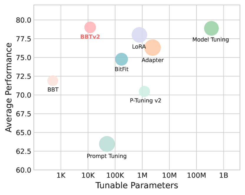
Figure 1: BBTv2 achieves comparable results to gradient-based methods on average performance over 7 language understanding tasks (§5.1) with much fewer tunable parameters. Size of the circle is proportional to the standard deviation of the performance. All the methods are evaluated on RoBERTa_LARGE.

To make LLMs benefit a wider range of audiences, a common practice is to release LLMs as a service and allow users to access the powerful LLMs through their inference APIs Brown et al. (2020). In such a scenario, called Languaged-Model-as-a-Service (LMaaS) Sun et al. (2022b), users cannot access or tune model parameters but can only tune their prompts to accomplish language tasks of interest. Brown et al. (2020) propose to recast downstream tasks as a language modeling task and perform different tasks by conditioning on task-specific text prompts. Further, they demonstrate that LLMs exhibit an emergent ability of in-context learning, i.e., LLMs can learn to perform tasks with a few demonstrations provided in the input context without updating parameters. Nevertheless, its performance has been shown to highly depend on the choice of the prompt or the demonstrations Zhao et al. (2021); Liu et al. (2022) and still lags far behind full model tuning.

Recently, Sun et al. (2022b) proposed Black-Box Tuning (BBT), which optimizes continuous prompt by only accessing model inference APIs. In contrast to gradient-based tuning that requires expensive back-propagation, BBT only requires model forward computation, which can be highly optimized by acceleration frameworks such as ONNX Runetime and TensorRT. In addition, the optimization cost of BBT is decoupled from the scale of the model. Instead, larger models can be more favorable to BBT due to the lower intrinsic dimensionality Aghajanyan et al. (2021). Despite its efficiency superiority and comparable performance to gradient descent, our pilot experiments (§3) show that BBT lacks versatility across tasks and PTMs.

In this paper, we present BBTv2, an improved version of BBT, to address these issues. Instead of injecting continuous prompt tokens merely in the input layer, BBTv2 prepends prompts to hidden states at every layer of the PTM (termed as deep prompts), incorporating an order of magnitude more parameters to handle more difficult tasks. However, the increased number of parameters also poses a challenge for high-dimensional derivative-free optimization (DFO, Shahriari et al. (2016); Qian and Yu (2021)). Fortunately, we show that the forward computation of modern PTMs can be decomposed into an additive form w.r.t. hidden states of each layer thanks to the residual connections He et al. (2016). Hence, the optimization of the deep prompts can be decomposed into multiple low-dimensional sub-problems, each corresponding to the optimization of prompt at one layer. Based on this insight, we propose a divide-and-conquer algorithm to alternately optimize prompt at each layer. For the optimization at each layer, we maintain a random linear transformation that projects the prompt parameters into a low-dimensional subspace and perform DFO in the generated subspace. To generalize BBTv2 to a variety of PTMs, we generate the random projections using normal distributions with PTM-related standard deviations.

Experimental results show that BBTv2 significantly improves BBT on average performance across 7 language understanding tasks. As shown in Figure 1, BBTv2 achieves comparable performance to full model tuning and state-of-the-art PET methods including Adapter Houlsby et al. (2019), BitFit Zaken et al. (2022), LoRA Hu et al. (2021), and P-Tuning v2 Liu et al. (2021b) while with much fewer tunable parameters. Code is publicly available at https://github.com/txsun1997/Black-Box-Tuning.

2 Black-Box Tuning

Black-Box Tuning (BBT) Sun et al. (2022b) is a derivative-free framework to drive PTMs for few-shot learning. In particular, for a batch of training data $(X,Y)$, we first convert the texts $X$ with some pre-defined templates (e.g., "It was [MASK]") into $\tilde{X}$, and the labels $Y$ with a pre-defined map into label words $\tilde{Y}$ (e.g., "great" and "terrible"). By this, we can formulate various downstream tasks into a general-purpose (masked) language modeling task and utilize the pre-trained (masked) language modeling head to solve them. Assume the PTM inference API $f$ takes a continuous prompt $\mathbf{p}$ and a batch of converted texts $\tilde{X}$ as input, and outputs the logits of the tokens of interest (e.g., the [MASK] token). BBT seeks to find the optimal prompt $\mathbf{p}^{\star}=\arg\min_{\mathbf{p}\in\mathcal{P}}\mathcal{L}(f(\mathbf{p},\tilde{X}),\tilde{Y})$, where $\mathcal{P}$ is the prompt space and $\mathcal{L}$ is some loss function such as cross entropy. The closed form and the gradients of $f$ are not accessible to BBT.

The prompt $\mathbf{p}\in\mathbb{R}^{D}$ usually has tens of thousands of dimensions, making it infeasible to be optimized with derivative-free optimization (DFO) algorithms. Hence, BBT adopts a random projection $\mathbf{A}\in\mathbb{R}^{D\times d}$ to generate a low-dimensional subspace $\mathcal{Z}\in\mathbb{R}^{d}$ and performs optimization in the generated subspace, i.e.,

$$\mathbf{z}^{\star}=\mathop{\arg\min}_{\mathbf{z}\in\mathcal{Z}}\mathcal{L}(f(\mathbf{Az}+\mathbf{p}_{0},\tilde{X}),\tilde{Y}),$$ (1)

where $\mathbf{p}_{0}$ is the initial prompt embedding. If not using pre-trained prompt embedding, $\mathbf{p}_{0}$ is the word embeddings randomly drawn from the vocabulary.

BBT adopts the Covariance Matrix Adaptation Evolution Strategy (CMA-ES) Hansen and Ostermeier (2001); Hansen et al. (2003) to optimize Eq.(1) and obtain the desired prompt $\mathbf{p}^{\star}=\mathbf{A}\mathbf{z}^{\star}$. The random projection $\mathbf{A}$ is frozen during optimization.

3 Pilot Experiments

3.1 Limitations of BBT Across Tasks

Unsatisfactory Performance on Entailment Tasks.

As demonstrated by Sun et al. (2022b), BBT can outperform model tuning on entailment tasks when using pre-trained prompt embedding for initialization. However, pre-trained prompt embedding is not always available for many languages and PTMs. Without pre-trained prompt embedding, BBT still lags far behind model tuning on entailment tasks. In other words, BBT does not completely get rid of the dependence on gradients to exceed model tuning. In contrast, as depicted in Figure 2, BBTv2 can match the performance of model tuning on three entailment tasks, namely MRPC Dolan and Brockett (2005), SNLI Bowman et al. (2015), and RTE Wang et al. (2019) without using pre-trained prompt embedding.

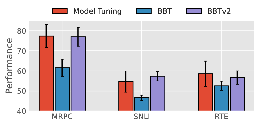
Figure 2: Performance on three entailment tasks. We report F1 score for MRPC and accuracy for SNLI and RTE. Without pre-trained prompt embedding, BBTv2 can still match the performance of full model tuning on entailment tasks under the 16-shot setting.

Slow Convergence on Many-Label Classification Tasks.

BBT suffers from slow convergence rate when the number of labels becomes large. As reported by Sun et al. (2022b), BBT cannot converge within the budget of 8,000 API calls, which is sufficient for common tasks to converge, on DBPedia Zhang et al. (2015), a topic classification task with 14 labels. Figure 3 shows the cross entropy loss and the training accuracy during optimization. Compared with BBT, the proposed BBTv2 significantly accelerates convergence on DBPedia.

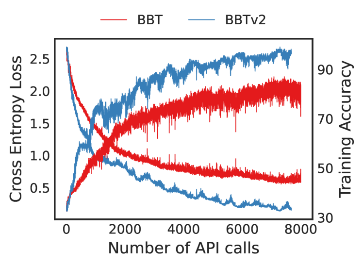
Figure 3: Comparison of the convergence rates of BBT and BBTv2 on DBPedia (14 classes).

3.2 Limitations of BBT Across PTMs

Overfitting on Training Data.

When switching the backbone model from RoBERTa Liu et al. (2019) to other PTMs, we find that BBT tends to overfit training data. As shown in Figure 4, the original BBT with BERT_LARGE Devlin et al. (2019) and BART_LARGE Lewis et al. (2020) can achieve 100% accuracy on the SST-2 training set, but achieves little improvement on the development set. We conjecture that the random projection adopted by the original BBT hinders its generalization. By generating random projections using normal distributions with model-related standard deviations (§4.2), our modified BBT and BBTv2 exhibit stronger generalization ability.

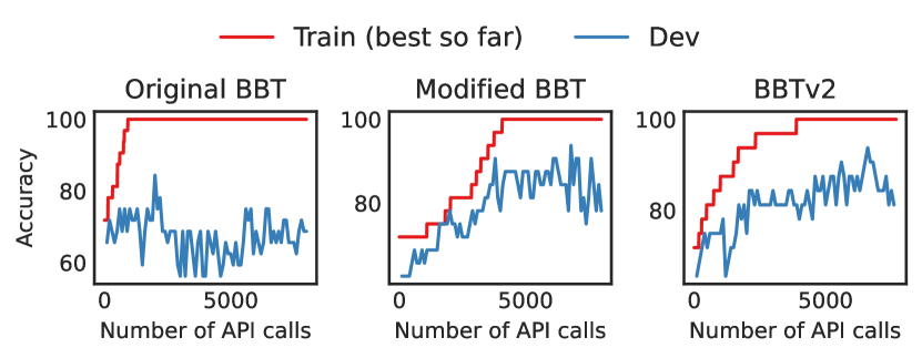
(a) BERT_LARGE

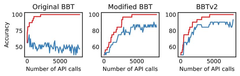
(b) BART_LARGE

Figure 4: Accuracy on the 16-shot training and development set of SST-2 with BERT_LARGE and BART_LARGE. The original BBT tends to overfit training data. By using normal distributions with the standard deviations calculated by Eq.(6) to generate random projections, the modified BBT and BBTv2 can generalize well to development sets.

4 BBTv2

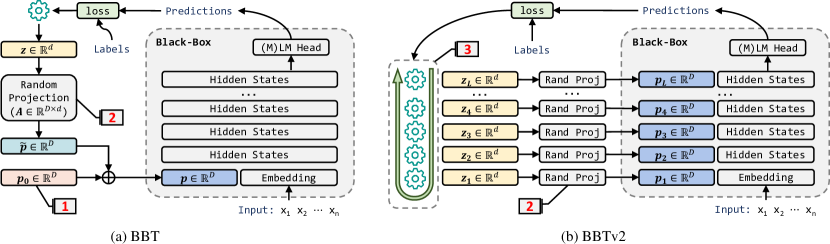
Figure 5: An illustration of (a) BBT Sun et al. (2022b) and (b) BBTv2.   is some derivative-free optimizer such as CMA-ES. Compared with BBT, BBTv2 has 3 differences: (1) BBT requires pre-trained prompt embedding $\mathbf{p}_{0}$ to match the performance of model tuning on entailment tasks, and therefore does not completely get rid of gradients. In contrast, BBTv2 requires no prompt pre-training. (2) BBT generates the random projection using a uniform distribution while BBTv2 adopts model-specific normal distributions. (3) Instead of optimizing the prompt merely in the input layer, BBTv2 uses a divide-and-conquer algorithm to alternately optimize prompt at each layer.

0:  $L$-layer PTM Inference API $f$,

          Loss function $\mathcal{L}$,

          Budget of API calls $\mathcal{B}$,

          Derivative-free optimizers $\{\mathcal{M}_{j}\}_{j=1}^{L}$

1:  Initialize random projections $\mathbf{A}_{1},\dots,\mathbf{A}_{L}$

2:  Initialize parameters $\mathbf{z}_{1}^{(0)},\dots,\mathbf{z}_{L}^{(0)}$

3:  Deep prompts $\mathbf{p}=\langle\mathbf{A}_{1}\mathbf{z}_{1}^{(0)},\dots,\mathbf{A}_{L}\mathbf{z}_{L}^{(0)}\rangle$

4:  for $i=1$ to $\mathcal{B}/L$ do

5:     for $j=1$ to $L$ do

6:        Evaluate: $loss=\mathcal{L}(f(\mathbf{p}))$

7:        Update: $\mathbf{z}_{j}^{(i)}\leftarrow\mathcal{M}_{j}(\mathbf{z}_{j}^{(i-1)},loss)$

8:        Replace: $\mathbf{p}_{j}\leftarrow\mathbf{A}_{j}\mathbf{z}_{j}^{(i)}$

9:     end for

10:  end for

11:  return Optimized deep prompts $\mathbf{p}$

Algorithm 1 DC Algorithm for BBTv2

4.1 Deep Black-Box Tuning

Though BBT has achieved comparable performance to model tuning on simple classification tasks (e.g., SST-2), our pilot experiments (§3) show that it lacks versatility across tasks and PTMs. As an improved variant of BBT, BBTv2 seeks to generalize BBT across tasks and PTMs.

Inspired by the recent success of deep prompt tuning (Li and Liang, 2021; Qin and Eisner, 2021; Liu et al., 2021b), we manage to inject continuous prompt tokens to every layer of the PTM and optimize them with derivative-free methods. Compared to BBT that optimizes the prompt merely in the input layer, BBTv2 has an order of magnitude more parameters. For a PTM with $L$ layers, BBTv2 seeks to optimize $\mathbf{p}=\langle\mathbf{p}_{1},\dots,\mathbf{p}_{L}\rangle$, where $\mathbf{p}_{i}\in\mathbb{R}^{D}$. Hence, the number of parameters to be optimized becomes $LD$. Say we are using RoBERTa_LARGE with 24 layers and insert 50 prompt tokens at each layer, the total number of parameters to be optimized is 1.2M, posing a challenge of high-dimensional DFO. Instead of simply extending the dimensionality of the random projection matrix $\mathbf{A}$ to $\mathbb{R}^{LD\times d}$ , we propose a divide-and-conquer (DC) algorithm to handle the increased parameters.

In fact, DC has been well explored in prior work Kandasamy et al. (2015); Mei et al. (2016) to cope with high-dimensional DFO problems by decomposing the original high-dimensional problem into multiple low-dimensional sub-problems, and solving them separately. The key assumption of applying DC is that, the objective $f$ can be decomposed into some additive form. Fortunately, the forward computation of modern PTMs can be expanded into an additive form due to the residual connections He et al. (2016). For instance, the forward computation of a three-layered PTM can be decomposed as

$$f(\mathbf{x}_{1}) =f_{3}(\mathbf{x}_{3})+\mathbf{x}_{3}$$ (2)

$$=f_{3}(\mathbf{x}_{3})+f_{2}(\mathbf{x}_{2})+\mathbf{x}_{2}$$ (3)

$$=f_{3}(\mathbf{x}_{3})+f_{2}(\mathbf{x}_{2})+f_{1}(\mathbf{x}_{1})+\mathbf{x}_{1},$$ (4)

where $f_{i}$ is the transformation function of the $i$-th layer, $\mathbf{x}_{i}$ is the input of the $i$-th layer, and $\mathbf{x}_{1}$ is the input embedding. Thus, optimizing the continuous prompts $\{\mathbf{p}_{i}\}_{i=1}^{L}$ attached to the hidden states at every layer $\{\mathbf{x}_{i}\}_{i=1}^{L}$ can be regarded as independent sub-problems. Since the assumption is satisfied, we propose a DC-based algorithm, which is described in Algorithm 1, to implement BBTv2.

The prompts at different layers are optimized alternately from bottom to up. For the optimization at each layer, we maintain a specific random projection $\mathbf{A}_{j}$ and a CMA-ES optimizer $\mathcal{M}_{j}$. When alternating to layer $j$ (Line 6-8 in Algorithm 1), a single CMA-ES iteration is performed in the same fashion as BBT, i.e., a new $\mathbf{z}_{j}$ is generated by $\mathcal{M}_{j}$ and is then projected to $\mathbf{p}_{j}$ using $\mathbf{A}_{j}$. A graphical illustration is shown in Figure 5.

During PTM inference, $\mathbf{p}_{j}=\mathbf{A}_{j}\mathbf{z}_{j}$ is first added with an initial prompt embedding $\mathbf{p}_{j}^{0}$ and then concatenated with the hidden states $\mathbf{x}_{j}$. Thus, according to Eq.(4), the forward computation of a $L$-layered PTM can be viewed as

$$f(\mathbf{x}_{1},\mathbf{p}_{1:L})= [\mathbf{A}_{1}{\color[rgb]{1,0.23,0.13}{\mathbf{z}_{1}}}+\mathbf{p}_{1}^{0};\mathbf{x}_{1}]$$

$$+\sum_{j=1}^{L}f_{j}([\mathbf{A}_{j}{\color[rgb]{1,0.23,0.13}{\mathbf{z}_{j}}}+\mathbf{p}_{j}^{0};\mathbf{x}_{j}]),$$ (5)

where $[\cdot;\cdot]$ means concatenation. Tunable parameters are highlighted in color. We set $\mathbf{p}_{1}^{0}$ as the word embeddings randomly drawn from the PTM vocabulary for all tasks. $\mathbf{p}_{j}^{0}$ ($1<j\leq L$) is the hidden states of the prompt tokens at the $j$-th layer.

4.2 Revisiting Random Projection

In the original BBT, each entry in the random projection $\mathbf{A}$ is sampled from a uniform distribution He et al. (2015). In their experiments, using normal distribution $\mathcal{N}(0,1/d)$ to generate the random projection results in slow convergence and inferior performance. However, we show in pilot experiments that the uniform distribution exhibits poor generalization on PTMs other than RoBERTa. In this section, we shed some light on the effect of the random projection, and propose to use normal distributions with model-related standard deviations to generate random projections. In fact, most prior works in high-dimensional DFO Wang et al. (2016); Qian et al. (2016) also adopt normal distributions to generate random projections. However, they usually simply use $\mathcal{N}(0,1)$ or $\mathcal{N}(0,1/d)$, both of which underperform in our scenario.

To take a closer look into the effect of the random projection, we draw distribution of the initial prompt $\mathbf{p}$ that is projected from $\mathbf{z}$ by the projection matrix $\mathbf{A}$. Here, $\mathbf{z}$ is sampled from the normal distribution maintained by the CMA-ES, which is initially set to $\mathcal{N}(0,0.5)$ in BBT. By generating $\mathbf{A}$ from different distributions, we simulate the distribution of the projected prompt $\mathbf{p}$ and compare with the distribution of RoBERTa_LARGE word embeddings. As revealed by Figure 6, when $\mathbf{A}$ is sampled from the normal distribution used in the original BBT, i.e., $\mathcal{N}(0,1/d)$, the projected prompt $\mathbf{p}$ cannot cover the range of word embeddings, and therefore suffers from slow convergence. In contrast, using uniform distribution can cover the range of word embeddings, which explains why it performs well on RoBERTa_LARGE.

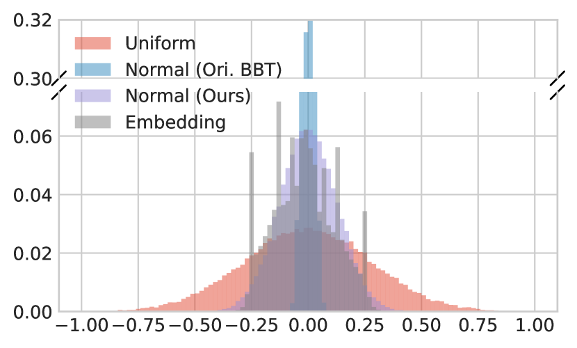
Figure 6: Distributions of RoBERTa word embeddings and generated prompt $\mathbf{p}=\mathbf{Az}$ where $\mathbf{A}$ is sampled from different distributions. When using our designed normal distribution to generate the random projection $\mathbf{A}$, the distribution of the projected prompt well matches the shape of the word embedding distribution, leading to faster convergence and stronger generalization.

Thus, to generalize BBT (and BBTv2) across different PTMs, we have to take into account the distribution of word embeddings (and hidden states for BBTv2) of the PTM for generating random projections. In particular, we use the normal distribution with standard deviation as follows,

$$\sigma_{A}=\frac{\alpha\hat{\sigma}}{\sqrt{d}\sigma_{z}},$$ (6)

where $\hat{\sigma}$ is observed standard deviation of word embeddings (or hidden states for BBTv2), $\sigma_{z}$ is the standard deviation of the normal distribution maintained by CMA-ES, $\alpha$ is a constant scalar to stretch the distribution. Initially, we set $\mu_{z}=\mu_{A}=0$ so that no prior knowledge about the optimization direction is incorporated. The main idea behind the above calculation is to match the distribution (more specifically the variance) between the projected prompt and word embeddings (or hidden states). When $\alpha=1$, as we can see in Figure  6, the distribution of the projected prompt can perfectly match the distribution of the word embeddings. Detailed derivation of Eq.(6) is provided in Appendix A.

5 Experiments

Method	Tunable	SST-2	Yelp P.	AG’s News	DBPedia	MRPC	SNLI	RTE	Avg.
	Params	acc	acc	acc	acc	F1	acc	acc
Gradient-Based Methods
Model Tuning	355M	85.39 $\pm$2.84	91.82 $\pm$0.79	86.36 $\pm$1.85	97.98 $\pm$0.14	77.35 $\pm$5.70	54.64 $\pm$5.29	58.60 $\pm$6.21	78.88
Adapter	2.4M	83.91 $\pm$2.90	90.99 $\pm$2.86	86.01 $\pm$2.18	97.99 $\pm$0.07	69.20 $\pm$3.58	57.46 $\pm$6.63	48.62 $\pm$4.74	76.31
BitFit	172K	81.19 $\pm$6.08	88.63 $\pm$6.69	86.83 $\pm$0.62	94.42 $\pm$0.94	66.26 $\pm$6.81	53.42 $\pm$10.63	52.59 $\pm$5.31	74.76
LoRA	786K	88.49 $\pm$2.90	90.21 $\pm$4.00	87.09 $\pm$0.85	97.86 $\pm$0.17	72.14 $\pm$2.23	61.03 $\pm$8.55	49.22 $\pm$5.12	78.01
Prompt Tuning	50K	68.23 $\pm$3.78	61.02 $\pm$6.65	84.81 $\pm$0.66	87.75 $\pm$1.48	51.61 $\pm$8.67	36.13 $\pm$1.51	54.69 $\pm$3.79	63.46
P-Tuning v2	1.2M	64.33 $\pm$3.05	92.63 $\pm$1.39	83.46 $\pm$1.01	97.05 $\pm$0.41	68.14 $\pm$3.89	36.89 $\pm$0.79	50.78 $\pm$2.28	70.47
Gradient-Free Methods
Manual Prompt	0	79.82	89.65	76.96	41.33	67.40	31.11	51.62	62.56
In-Context Learning	0	79.79 $\pm$3.06	85.38 $\pm$3.92	62.21 $\pm$13.46	34.83 $\pm$7.59	45.81 $\pm$6.67	47.11 $\pm$0.63	60.36 $\pm$1.56	59.36
Feature-MLP	1M	64.80 $\pm$1.78	79.20 $\pm$2.26	70.77 $\pm$0.67	87.78 $\pm$0.61	68.40 $\pm$0.86	42.01 $\pm$0.33	53.43 $\pm$1.57	66.63
Feature-BiLSTM	17M	65.95 $\pm$0.99	74.68 $\pm$0.10	77.28 $\pm$2.83	90.37 $\pm$3.10	71.55 $\pm$7.10	46.02 $\pm$0.38	52.17 $\pm$0.25	68.29
BBT	500	89.56 $\pm$0.25	91.50 $\pm$0.16	81.51 $\pm$0.79	79.99⋆$\pm$2.95	61.56 $\pm$4.34	46.58 $\pm$1.33	52.59 $\pm$2.21	71.90
BBTv2	12K	90.33 $\pm$1.73	92.86 $\pm$0.62	85.28 $\pm$0.49	93.64 $\pm$0.68	77.01 $\pm$4.73	57.27 $\pm$2.27	56.68 $\pm$3.32	79.01

Table 1: Overall comparison on various language understanding tasks. We report mean and standard deviation of performance over 3 different splits (§5.1). All of the results are obtained with pre-trained RoBERTa_LARGE in the 16-shot (per class) setting. In each track, the best results are highlighted in bold and the second best results are marked with underline. ^⋆ We reimplement BBT on DBPedia given a budget of 8,000 API calls for fair comparison.

5.1 Datasets and Tasks

For comparison, we evaluate BBTv2 on the same datasets as BBT, i.e., SST-2 Socher et al. (2013), Yelp Zhang et al. (2015), AG’s News Zhang et al. (2015), DBPedia Zhang et al. (2015), SNLI Bowman et al. (2015), RTE Wang et al. (2019), and MRPC Dolan and Brockett (2005). SST-2 and Yelp are sentiment analysis tasks, AG’s News and DBPedia are topic classification tasks, SNLI and RTE are natural language inference (NLI) tasks, and MRPC is a paraphrase task. In addition, we include two Chinese tasks, ChnSent and LCQMC Liu et al. (2018), for evaluation on CPM-2 Zhang et al. (2021b), a Chinese PTM with $\sim$11B parameters. ChnSent is a sentiment analysis task while LCQMC is a question matching task.

We follow the same procedure as Zhang et al. (2021a); Gu et al. (2021); Sun et al. (2022b) to construct the true few-shot learning settings Perez et al. (2021). In particular, we randomly draw $k$ samples for each class to construct a $k$-shot training set $\mathcal{D}_{\text{train}}$, and construct a development set $\mathcal{D}_{\text{dev}}$ by randomly selecting another $k$ samples from the original training set such that $|\mathcal{D}_{\text{train}}|=|\mathcal{D}_{\text{dev}}|$. We use the original development sets as the test sets. For datasets without development sets, we use the original test sets. Therefore, in our experiments we have $|\mathcal{D}_{\text{test}}|\gg|\mathcal{D}_{\text{train}}|=|\mathcal{D}_{\text{dev}}|$.

5.2 Baselines

We consider two types of methods as our baselines: gradient-based methods and gradient-free methods.

For gradient-based methods, we compare with (1) Model Tuning and state-of-the-art parameter-efficient methods including (2) Adapter Houlsby et al. (2019), (3) BitFit Zaken et al. (2022), (4) LoRA Hu et al. (2021), (5) Prompt Tuning Lester et al. (2021), and (6) P-Tuning v2 Liu et al. (2021b). We implement Adapter, BitFit, and LoRA using OpenDelta, and evaluate P-Tuning v2 in our experimental settings based on the official implementation. The results of Model Tuning and Prompt Tuning are taken from Sun et al. (2022b).

For gradient-free methods, we compare with two non-learning prompt-based methods: (1) Manual Prompt and (2) In-Context Learning Brown et al. (2020); two feature-based methods: (3) Feature-MLP and (4) Feature-BiLSTM, which is to train a MLP/BiLSTM classifier on the features extracted by the PTM; and (5) BBT Sun et al. (2022b). The results of these gradient-free baselines are taken from Sun et al. (2022b). One exception is the performance of BBT on DBPedia. In the original paper, BBT is performed given a larger budget (20,000 API calls) on DBPedia for convergence. In this work, we reimplement BBT on DBPedia with the same budget (8,000 API calls) as other tasks for fair comparison.

5.3 Implementation Details

Backbones.

To compare with BBT, we mainly use RoBERTa_LARGE Liu et al. (2019) as our backbone model. To verify the versatility, we also evaluate on other PTMs including BERT_LARGE Devlin et al. (2019), GPT-2_LARGE, BART_LARGE Lewis et al. (2020), and T5_LARGE Raffel et al. (2020). In addition, we also evaluate BBTv2 on a supersized Chinese PTM, CPM-2 Zhang et al. (2021b), which has $\sim$11B parameters.

Hyperparameters.

Most of the hyperparameters remain the same as BBT. We insert 50 continuous prompt tokens at each layer. The subspace dimensionality is set to 500. The CMA-ES with population size of 20 and budget of 8,000 API calls is applied to all the tasks. We adopt cross entropy as the loss function. For generating random projections, we use normal distributions with standard deviations calculated by Eq.(6) instead of uniform distributions.

	SST-2		AG’s News
	(max seq len: 47)		(max seq len: 107)
	BBT	BBTv2	BBT	BBTv2
Accuracy	89.4	91.4	82.6	85.5
Training Time
PyTorch (mins)	14.8	11.0	28.3	25.0
ONNX (mins)	6.1	4.6	17.7	10.4
Memory
User (MB)	30	143	30	143
Server (GB)	3.0	3.0	4.6	4.6
Network
Upload (KB)	6	52	22	68
Download (KB)	0.25	0.25	1	1

Table 2: Comparison of BBT and BBTv2 on accuracy, training time, memory use, and network load.

5.4 Results

Overall Comparison.

As shown in Table 1, BBTv2 outperforms BBT and other gradient-free methods on 6/7 tasks. In contrast to BBT, the improvement of BBTv2 mainly comes from DBPedia, which has 14 classes, and hard entailment tasks, namely MRPC and SNLI. On simple tasks such as SST-2 and Yelp, BBT can perform on par with BBTv2. When compared with gradient-based methods, BBTv2 achieves the best result in average across the 7 tasks while maintaining much fewer tunable parameters. It is worth noting that BBTv2, without any gradient-based components (e.g., the pre-trained prompt embedding used in BBT on entailment tasks Sun et al. (2022b) or the white-box prompt optimization required by Diao et al. (2022)), is the first pure black-box method that matches the performance of full model tuning on various understanding tasks.

Detailed Comparison.

In Table 2, we compare BBTv2 with BBT in other dimensions than accuracy. In addition to the improvement in accuracy, BBTv2 also confers faster convergence than BBT. For fair comparison of training time, we perform early stopping if the development accuracy does not increase after 1,000 steps. We report training times under two implementations, PyTorch Paszke et al. (2019) and ONNX Runtime, on a single NVIDIA GTX 3090 GPU. In terms of memory footprint and network load, BBTv2 slightly increases the memory use on the user side and the amount of data to be uploaded.

BBTv2 Across PTMs.

To verify the universality of BBTv2 across PTMs, we also evaluate on BERT, GPT-2, BART, T5, and CPM-2. As shown in Table 3, BBTv2 achieves superior performance over BBT on PTMs with varying architectures, i.e., encoder-only, decoder-only, and encoder-decoder PTMs. In addition, we also verify the effectiveness of BBTv2 on a supersized Chinese PTM, CPM-2, which has $\sim$11B parameters. As shown in Table 4, when using CPM-2 as the backbone, BBTv2 outperforms full model tuning on two Chinese tasks. The results of Vanilla PT, Hybrid PT, and LM Adaption, which are three variants of prompt tuning, are taken from Gu et al. (2021).

LM	Method	SST-2	AG’s News	DBPedia
Encoder-only PTMs
BERT	BBT	76.26 $\pm$2.64	76.67 $\pm$1.12	89.58 $\pm$0.51
	BBTv2	79.32 $\pm$0.29	79.58 $\pm$1.15	93.74 $\pm$0.50
RoBERTa	BBT	89.56 $\pm$0.25	81.51 $\pm$0.79	79.99 $\pm$2.95
	BBTv2	90.33 $\pm$1.73	85.28 $\pm$0.49	93.64 $\pm$0.68
Decoder-only PTMs
GPT-2	BBT	75.53 $\pm$1.98	77.63 $\pm$1.89	77.46 $\pm$0.69
	BBTv2	83.72 $\pm$3.05	79.96 $\pm$0.75	91.36 $\pm$0.73
Encoder-Decoder PTMs
BART	BBT	77.87 $\pm$2.57	77.70 $\pm$2.46	79.64 $\pm$1.55
	BBTv2	89.53 $\pm$2.02	81.30 $\pm$2.58	87.10 $\pm$2.01
T5	BBT	89.15 $\pm$2.01	83.98 $\pm$1.87	92.76 $\pm$0.83
	BBTv2	91.40 $\pm$1.17	85.11 $\pm$1.11	93.36 $\pm$0.80

Table 3: Comparison of BBT and BBTv2 on the large versions of BERT, RoBERTa, GPT-2, BART and T5.

Method	Tunable	ChnSent	LCQMC
	Params	acc	acc
Model Tuning	11B	86.1 $\pm$1.8	58.8 $\pm$1.8
Vanilla PT	410K	62.1 $\pm$3.1	51.5 $\pm$3.4
Hybrid PT	410K	79.2 $\pm$4.0	54.6 $\pm$2.3
LM Adaption	410K	74.3 $\pm$5.2	51.4 $\pm$2.9
BBTv2	4.8K	86.4 $\pm$0.8	59.1 $\pm$2.5

Table 4: Results on two Chinese tasks with CPM-2 as the backbone PTM.

5.5 Ablations

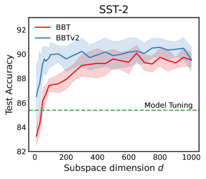
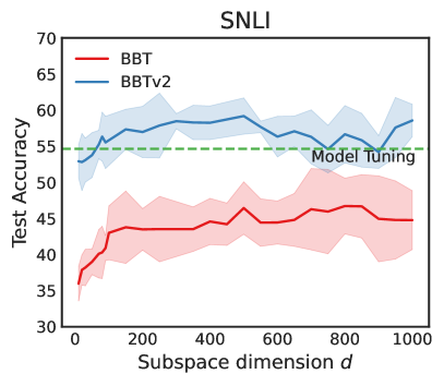
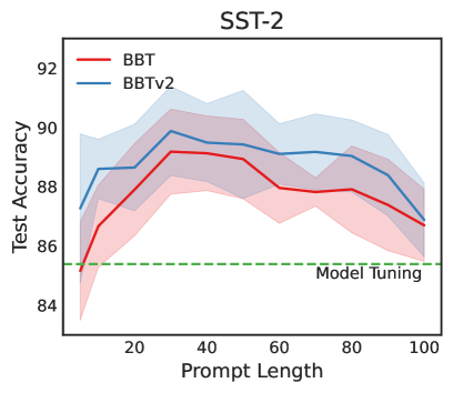
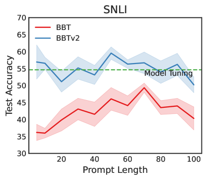
Figure 7: Ablation results on subspace dimensionality and prompt length. We show mean and standard deviation of performance over 5 different runs.

Effect of Subspace Dimensionality.

We explore the subspace dimensionality $d$ from 10 to 1000 using both BBT and BBTv2. The population size is set to $\lambda=4+3\log(d)$ accordingly. Experimental results on SST-2 and SNLI are demonstrated in Figure 7, from which we observe that: (1) Increasing subspace dimensionality $d$ generally confers improved performance for both BBT and BBTv2, but marginal effect is also observed when $d>100$; (2) BBTv2 almost always performs better than BBT with the same subspace dimensionality.

Effect of Prompt Length.

As reported in prior work Lester et al. (2021); Sun et al. (2022b), prompt length can be a sensitive hyperparameter to model performance. Hence, we explore the prompt length from 5 to 100 using BBT and BBTv2. As shown in Figure 7: (1) The optimal prompt length lies in the range from 5 to 100 and varies across tasks; (2) The effect of prompt length is somehow consistent between BBT and BBTv2.

Effect of Model Scale.

It has been demonstrated that larger PTMs have a lower intrinsic dimensionality Aghajanyan et al. (2021) and therefore, BBT and BBTv2 should be more favorable to larger PTMs. To verify this, we conduct experiments on AG’s News using T5 Raffel et al. (2020) with varying scales, i.e., T5_SMALL, T5_BASE, T5_LARGE, and T5_XL, corresponding to 60M, 220M, 740M, and 3B parameters. As shown in Figure 8, in the AG’s News 16-shot learning setting, the gradient-based counterpart, namely deep prompt tuning (DPT, Li and Liang (2021); Liu et al. (2021b); Qin and Eisner (2021)), performs better than BBT and BBTv2 on T5_SMALL and T5_BASE. When using T5_LARGE and T5_XL, black-box tuning outperforms DPT, demonstrating its power of scale.

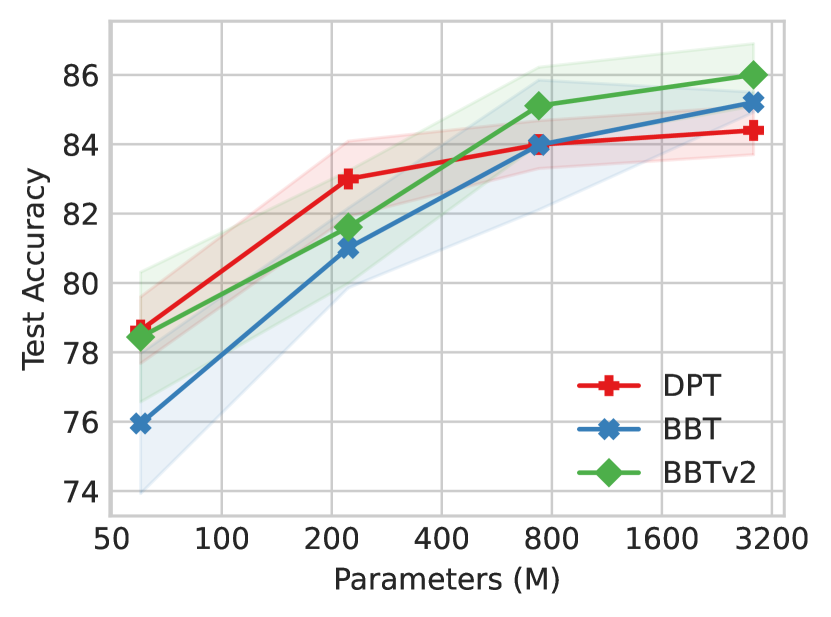
Figure 8: The power of scale for black-box tuning with T5 on AG’s News. DPT: deep prompt tuning.

6 Related Work

Parameter-Efficient Tuning (PET).

PET is to optimize only a small portion of parameters while keeping the main body of the model unchanged. PET has achieved comparable performance to full model tuning when training data is sufficient He et al. (2021). The tunable parameters can be injected into different positions of the PTM. Houlsby et al. (2019) insert lightweight adapters to each PTM layer; Lester et al. (2021) prepend continuous prompt tokens to the input layer; Li and Liang (2021); Liu et al. (2021b) inject tunable prompt tokens to hidden states of every layer; Zaken et al. (2022) only optimize the bias-terms in the PTM; Hu et al. (2021) learn to adapt attention weights via low-rank matrices. Though the number of tunable parameters is reduced, back-propagation through the entire model is still required to calculate the gradients to update the small portion of parameters. To that end, gradient-free methods are also proposed to optimize continuous prompt Sun et al. (2022b); Diao et al. (2022) or discrete prompt Prasad et al. (2022); Deng et al. (2022).

Prompt-Based Learning.

Prompt-based learning is to formulate downstream tasks as a (masked) language modeling task, and therefore reduces the gap between PTM pre-training and fine-tuning Liu et al. (2021a); Sun et al. (2022a). The prompt can be manually designed Brown et al. (2020); Schick et al. (2020); Schick and Schütze (2021), mined from corpora Jiang et al. (2020), generated by generative PTMs Gao et al. (2021), or be constructed using gradient-guided search Shin et al. (2020). In this work, we also insert manually crafted textual prompts into input samples but only optimize the prepended continuous prompt tokens.

7 Conclusion

In this work, we present BBTv2, an improved version of BBT Sun et al. (2022b) with deep prompts that are attached to every layer of the PTM. To optimize the high-dimensional prompt parameters, we propose a divide-and-conquer (DC) algorithm combined with random projections to alternately optimize the continuous prompt at each layer. Experimental results demonstrate that BBTv2, without any gradient-based component, can achieve comparable performance to state-of-the-art PET methods and full model tuning while maintaining much fewer tunable parameters.

Limitations

We summarize the limitations of this work as follows: (1) BBTv2 adopts a divide-and-conquer algorithm to alternately optimize prompt at each PTM layer. We use a unique CMA-ES optimizer, which has two hyperparameters $\mu_{z}$ and $\sigma_{z}$, for the optimization at each layer. As mentioned previously, we set $\mu_{z}=0$ for not incorporating any prior to the optimization direction. Therefore, we have totally $L$ (number of layers) hyperparameters for optimization, i.e., $[\sigma_{z}^{(1)},\dots,\sigma_{z}^{(L)}]$. For simplicity, we constrain the $\sigma_{z}$ at different layers to be identical, i.e., $\sigma_{z}^{(1)}=\sigma_{z}^{(2)}=\cdots=\sigma_{z}^{(L)}$. In addition, Eq.(6) introduces another hyperparameter $\alpha$, which can also be different across different layers. Similarly, we constrain $\alpha$ at all layers to be identical. Hence, in contrast to BBT that has only one hyperparameter for optimization, BBTv2 introduces an additional hyperparameter and therefore increases the cost for hyperparameter search. (2) We conduct experiments on 9 language understanding tasks across 4 types (i.e., sentiment analysis, topic classification, paraphrasing, and natural language inference) and 2 languages (i.e., English and Chinese). However, the performance of BBTv2 on a wider range of understanding tasks and generation tasks is still under-explored. (3) We limit our work to few-shot learning because the training data can be wrapped into a single batch to be fed into the PTM such that the model inference API is a deterministic function whose output only depends on the prompt. In such a low-noise scenario, we can adopt the CMA-ES to successfully perform optimization. In the full data setting where the training samples are divided into mini-batches, we need to explore other derivative-free optimizers to handle the stochastic (noisy) optimization. We leave the investigation of adapting BBTv2 to a wider range of tasks and to full data settings as future work, further removing the remaining barriers to a gradient-free future.

Appendix A Deviation of $\sigma$ for Normal Distribution

Assume the variable $\mathbf{z}\in\mathbb{R}^{d}$ is sampled from a normal distribution $\mathcal{N}(\mu_{z},\sigma_{z})$ that is maintained by the CMA-ES, the random projection $\mathbf{A}\in\mathbb{R}^{D\times d}$ is generated from another normal distribution $\mathcal{N}(\mu_{A},\sigma_{A})$. Considering each entry of the prompt $\mathbf{p}_{ij}=\sum_{k}\mathbf{A}_{ik}\mathbf{z}_{kj}$, the variance is as follows,

$$\mathbb{V}(\sum_{k=1}^{d}\mathbf{A}_{ik}\mathbf{z}_{kj})=\sum_{k=1}^{d}\mathbb{V}(\mathbf{A}_{ik}\mathbf{z}_{kj})$$

$$\ \ \ \ \ \ \ \ +2\sum_{k=1}^{d-1}\sum_{p=k+1}^{d}\mathbb{C}\text{ov}(\mathbf{A}_{ik}\mathbf{z}_{kj},\mathbf{A}_{ip}\mathbf{z}_{pj}).$$ (7)

Since $\mathbf{A}$ and $\mathbf{z}$, and each entry in $\mathbf{A}$ and $\mathbf{z}$ are independent random variables and therefore the variance of $\sum_{k}\mathbf{A}_{ik}\mathbf{z}_{kj}$ can be simplified as

$$\mathbb{V}(\sum_{k=1}^{d}\mathbf{A}_{ik}\mathbf{z}_{kj}) =\sum_{k=1}^{d}\mathbb{V}(\mathbf{A}_{ik}\mathbf{z}_{kj})$$ (8)

$$=d\mathbb{V}(\mathbf{A}_{ik}\mathbf{z}_{kj}).$$ (9)

It is easy to obtain that

$$\mathbb{V}(\mathbf{A}_{ik}\mathbf{z}_{kj})= \mathbb{V}(\mathbf{A}_{ik})\mathbb{V}(\mathbf{z}_{kj})+\mathbb{V}(\mathbf{A}_{ik})(\mathbb{E}[\mathbf{z}_{kj}])^{2}$$

$$+\mathbb{V}(\mathbf{z}_{kj})(\mathbb{E}[\mathbf{A}_{ik}])^{2}$$ (10)

$$= \sigma_{A}^{2}\sigma_{z}^{2}+\sigma_{A}^{2}\mu_{z}^{2}+\sigma_{z}^{2}\mu_{A}^{2}.$$ (11)

Initially, we do not incorporate any prior on the optimization direction of the embedding (or hidden states) and therefore $\mu_{A}=\mu_{z}=0$. So we have $\mathbb{V}(\mathbf{A}_{ik}\mathbf{z}_{kj})=\sigma_{A}^{2}\sigma_{z}^{2}$. Combined with Eq.(9), the variance of the entries in the randomly projected prompt is as follows,

$$\mathbb{V}(\mathbf{p}_{ij})=d\sigma_{A}^{2}\sigma_{z}^{2}.$$ (12)

Ideally, we expect the generated prompt to lie in a reasonable solution space (e.g., the space of the embedding or hidden states) such that the embedding (hidden states) added by the prompt can still lie in a reasonable space. A natural idea is to match the variance of the generated prompt $\mathbf{p}$ and the embedding (or hidden states). Formally, we expect that $\mathbb{V}(\mathbf{p}_{ij})=(\alpha\hat{\sigma})^{2}$, where $\hat{\sigma}$ is the observed standard deviation of the embedding (or hidden states) and $\alpha$ is a constant scalar that controls the range (relative to that of the embedding or hidden states) where $\mathbf{p}$ falls in. We can obtain a recommendation value of the standard deviation of the random projection, that is

$$\sigma_{A}=\frac{\alpha\hat{\sigma}}{\sqrt{d}\sigma_{z}}.$$ (13)

In practice, $\alpha$ and $\sigma_{z}$ are hyperparameters. It is worth noting that the random projections are static during the optimization process and therefore we only need to observe the standard deviation of the word embeddings and the hidden states at every layer once at the beginning of the optimization. A possible concern is that such observation breaks the black-box and therefore it may be controversial to call it "black-box tuning". We take a perspective of feature-based approaches that views the embeddings and hidden states as features, which are the outputs of the model. Thus, we do not really access the inside information of the black-box model.

Appendix B Data Preprocessing

B.1 Statistics of Datasets

We list the statistics of the 7 English tasks and 2 Chinese tasks used in our experiments in Table 5. Among the 9 tasks, 5 are single-sentence classification tasks and 4 are sentence-pair classification tasks. The types of the tasks range from sentiment analysis, topic classification, paraphrase, and natural language inference (NLI).

Category	Dataset	Lang.	$\mid\mathcal{Y}\mid$	$\mid$Train$\mid$	$\mid$Test$\mid$	Type
single- sentence	SST-2	En	2	67k	0.9k	sentiment
	Yelp P.	En	2	560k	38k	sentiment
	AG’s News	En	4	120k	7.6k	topic
	DBPedia	En	14	560k	70k	topic
	ChnSent	Zh	2	6k	1.2k	sentiment
sentence- pair	MRPC	En	2	3.7k	0.4k	paraphrase
	RTE	En	2	2.5k	0.3k	NLI
	SNLI	En	3	549k	9.8k	NLI
	LCQMC	Zh	2	239k	8.8k	NLI

Table 5: Statistics of datasets used in our experiments. $\mid\mathcal{Y}\mid$: number of classes. "En" means English and "Zh" means Chinese.

B.2 Templates and Label Words

For both BBT and BBTv2, we convert input texts $X$ with pre-defined templates into $\tilde{X}$, and convert output labels $Y$ into label words $\tilde{Y}$, such that downstream tasks can be reformulated into a (masked) language modeling task and therefore we can reuse the pre-trained (masked) language modeling head. In Table 6, we list the input and output formats for different PTMs.

Dataset	Input	Output
Backbone: RoBERTa, BERT, BART
SST-2	$\langle P\rangle$ $\langle S\rangle$. It was [MASK]	great, bad
Yelp P.	$\langle P\rangle$ $\langle S\rangle$. It was [MASK]	great, bad
AG’s News	$\langle P\rangle$ [MASK] News: $\langle S\rangle$	World, Sports, Business, Tech
DBPedia	$\langle P\rangle$ [Category: [MASK]] $\langle S\rangle$	Company, Education, Artist, Athlete, Office, Transportation, Building,
		Natural, Village, Animal, Plant, Album, Film, Written
MRPC	$\langle P\rangle$ $\langle S_{1}\rangle$ ? [MASK], $\langle S_{2}\rangle$	Yes, No
RTE	$\langle P\rangle$ $\langle S_{1}\rangle$ ? [MASK], $\langle S_{2}\rangle$	Yes, No
SNLI	$\langle P\rangle$ $\langle S_{1}\rangle$ ? [MASK], $\langle S_{2}\rangle$	Yes, Maybe, No
Backbone: GPT-2
SST-2	$\langle P\rangle$ $\langle S\rangle$. The sentiment is	positive, negative
AG’s News	$\langle P\rangle$ $\langle S\rangle$. The news above is about	world, sports, business, tech
DBPedia	$\langle P\rangle$ $\langle S\rangle$. The text above is about	company, education, artist, athlete, office, transportation, building,
		natural, village, animal, plant, album, film, written
Backbone: T5
SST-2	$\langle P\rangle$ $\langle S\rangle$. It was [X]	[X] positive/negative
AG’s News	$\langle P\rangle$ [X] News: $\langle S\rangle$	[X] World/Sports/Business/Tech
DBPedia	$\langle P\rangle$ [Category: [X]] $\langle S\rangle$	[X] Company/Education/Artist/Athlete/Office/Transportation/Building/…
Backbone: CPM-2
ChnSent	$\langle P\rangle$ $\langle S\rangle$。总之很[X]。	[X] 好 / 差
LCQMC	$\langle P\rangle$ 判断：$\langle S_{1}\rangle$和$\langle S_{2}\rangle$两句话的意思是[X]的。	[X] 矛盾 / 相似

Table 6: Input templates and output label words used in our experiments. $\langle P\rangle$ is a sequence of continuous prompt tokens. $\langle S\rangle$ is the original input text. For BART, which outputs denoised input in an auto-regressive fashion, we only use the prediction of the masked position such that it follows the same output format as BERT and RoBERTa. For T5 and CPM-2, [X] is a special token similar to [MASK].

Appendix C Implementation Details

Clipping Hidden States

In practice, we find that the standard deviation $\hat{\sigma}$ of hidden states (especially at high layers) in some PTMs can be very large due to a few outliers. As a result, our calculated $\sigma_{A}$ (Eq.(6)) becomes large accordingly, and therefore the generated prompt has a wider range of values than expected. To address this issue, we iteratively clip hidden states into the range of $\hat{\mu}\pm 3\hat{\sigma}$. We perform clipping for 5 rounds and then compute the standard deviation $\hat{\sigma}$ of hidden states. Note that the clipping is only performed for statistics but is not applied during model forward compute.

Appendix D Additional Results

On Convergence of Normal Distributions

Previously in Figure 4, we show that using our designed normal distribution leads to better generalization from training data to development data. Nevertheless, as reported by Sun et al. (2022b), using normal distributions can suffer from slow convergence. Therefore, we compare the convergence rates using random projections generated from different distributions. As demonstrated in Figure 9: (1) For BBT, the convergence rate of using our designed normal distribution is significantly faster than the normal distribution used in the original BBT, and is comparable to uniform distribution; (2) For BBTv2, using our normal distribution converges more stably on both SST-2 and AG’s News. Especially, we observe that using our normal distribution converges faster than uniform distribution on AG’s News.

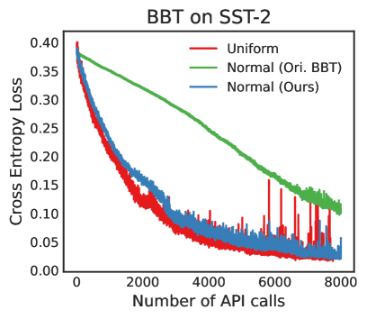
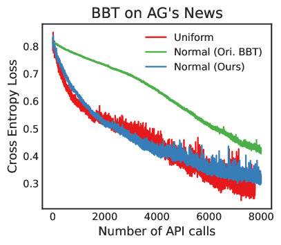
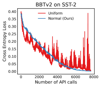
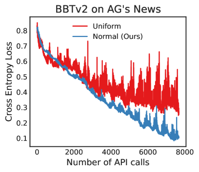
Figure 9: Comparison of convergence rates with random projections with different distributions. When using our designed normal distribution to generate random projections, both BBT and BBTv2 achieve fast and stable convergence.

Appendix E Estimation of Memory Use and Network Load

For measurement of memory footprint on user side, we use psutil to monitor CPU memory when running CMA-ES. For memory footprint on service side, we use nvidia-smi to monitor GPU memory when serving PTM inference.

For estimation of network load, we measure the amount of data to be uploaded and downloaded. For BBT and BBTv2, there are two kinds of data to be uploaded: (1) training samples, and (2) continuous prompt. A training sample is comprised of two parts: input_ids and attention_mask. We can use the unsigned short (representation range: 0$\sim$65535, 2 bytes per value) for input_ids and use the bool type (1 byte per value) for attention_mask. For continuous prompt, which contains hundreds of values for BBT or tens of thousands of values for BBTv2, we can use the float type (4 bytes per value) for representation. Take SST-2 16-shot split as an example, the input_ids and attention_mask are in shape of $32\times 47$, where 32 is the batch size and 47 is the maximum sequence length, so there are $\sim$2.9KB data for input_ids and $\sim$1.5KB data for attention_mask. Assume the subspace dimensionality is 500, we need to upload additional $\sim$2KB data for prompt if using BBT and $\sim$48KB data if using BBTv2. The data to be downloaded is the output logits of the candidate words, which is a dictionary containing $\mid\mathcal{Y}\mid$ float values. Take SST-2 16-shot split as an example, the size of data to be downloaded is $32\times 2\times 4\text{bytes}=0.25$KB. We assume the random projections are generated on the server side therefore there is no need to download hidden states to compute standard deviations for users.

References

- Aghajanyan et al. (2021) Armen Aghajanyan, Sonal Gupta, and Luke Zettlemoyer. 2021. Intrinsic dimensionality explains the effectiveness of language model fine-tuning. In Proceedings of the 59th Annual Meeting of the Association for Computational Linguistics and the 11th International Joint Conference on Natural Language Processing, ACL/IJCNLP 2021, (Volume 1: Long Papers), Virtual Event, August 1-6, 2021, pages 7319–7328. Association for Computational Linguistics.
- Bowman et al. (2015) Samuel R. Bowman, Gabor Angeli, Christopher Potts, and Christopher D. Manning. 2015. A large annotated corpus for learning natural language inference. In Proceedings of the 2015 Conference on Empirical Methods in Natural Language Processing, EMNLP 2015, Lisbon, Portugal, September 17-21, 2015, pages 632–642. The Association for Computational Linguistics.
- Brown et al. (2020) Tom B. Brown, Benjamin Mann, Nick Ryder, Melanie Subbiah, Jared Kaplan, Prafulla Dhariwal, Arvind Neelakantan, Pranav Shyam, Girish Sastry, Amanda Askell, Sandhini Agarwal, Ariel Herbert-Voss, Gretchen Krueger, Tom Henighan, Rewon Child, Aditya Ramesh, Daniel M. Ziegler, Jeffrey Wu, Clemens Winter, Christopher Hesse, Mark Chen, Eric Sigler, Mateusz Litwin, Scott Gray, Benjamin Chess, Jack Clark, Christopher Berner, Sam McCandlish, Alec Radford, Ilya Sutskever, and Dario Amodei. 2020. Language models are few-shot learners. In Advances in Neural Information Processing Systems 33: Annual Conference on Neural Information Processing Systems 2020, NeurIPS 2020, December 6-12, 2020, virtual.
- Deng et al. (2022) Mingkai Deng, Jianyu Wang, Cheng-Ping Hsieh, Yihan Wang, Han Guo, Tianmin Shu, Meng Song, Eric P. Xing, and Zhiting Hu. 2022. Rlprompt: Optimizing discrete text prompts with reinforcement learning. CoRR, abs/2205.12548.
- Devlin et al. (2019) Jacob Devlin, Ming-Wei Chang, Kenton Lee, and Kristina Toutanova. 2019. BERT: pre-training of deep bidirectional transformers for language understanding. In Proceedings of the 2019 Conference of the North American Chapter of the Association for Computational Linguistics: Human Language Technologies, NAACL-HLT 2019, Minneapolis, MN, USA, June 2-7, 2019, Volume 1 (Long and Short Papers), pages 4171–4186. Association for Computational Linguistics.
- Diao et al. (2022) Shizhe Diao, Xuechun Li, Yong Lin, Zhichao Huang, and Tong Zhang. 2022. Black-box prompt learning for pre-trained language models. CoRR, abs/2201.08531.
- Ding et al. (2022) Ning Ding, Yujia Qin, Guang Yang, Fuchao Wei, Zonghan Yang, Yusheng Su, Shengding Hu, Yulin Chen, Chi-Min Chan, Weize Chen, Jing Yi, Weilin Zhao, Xiaozhi Wang, Zhiyuan Liu, Hai-Tao Zheng, Jianfei Chen, Yang Liu, Jie Tang, Juanzi Li, and Maosong Sun. 2022. Delta tuning: A comprehensive study of parameter efficient methods for pre-trained language models. CoRR, abs/2203.06904.
- Dolan and Brockett (2005) William B. Dolan and Chris Brockett. 2005. Automatically constructing a corpus of sentential paraphrases. In Proceedings of the Third International Workshop on Paraphrasing, IWP@IJCNLP 2005, Jeju Island, Korea, October 2005, 2005. Asian Federation of Natural Language Processing.
- Gao et al. (2021) Tianyu Gao, Adam Fisch, and Danqi Chen. 2021. Making pre-trained language models better few-shot learners. In Proceedings of the 59th Annual Meeting of the Association for Computational Linguistics and the 11th International Joint Conference on Natural Language Processing, ACL/IJCNLP 2021, (Volume 1: Long Papers), Virtual Event, August 1-6, 2021, pages 3816–3830. Association for Computational Linguistics.
- Gu et al. (2021) Yuxian Gu, Xu Han, Zhiyuan Liu, and Minlie Huang. 2021. PPT: pre-trained prompt tuning for few-shot learning. CoRR, abs/2109.04332.
- Hansen et al. (2003) Nikolaus Hansen, Sibylle D. Müller, and Petros Koumoutsakos. 2003. Reducing the time complexity of the derandomized evolution strategy with covariance matrix adaptation (CMA-ES). Evol. Comput., 11(1):1–18.
- Hansen and Ostermeier (2001) Nikolaus Hansen and Andreas Ostermeier. 2001. Completely derandomized self-adaptation in evolution strategies. Evol. Comput., 9(2):159–195.
- He et al. (2021) Junxian He, Chunting Zhou, Xuezhe Ma, Taylor Berg-Kirkpatrick, and Graham Neubig. 2021. Towards a unified view of parameter-efficient transfer learning. CoRR, abs/2110.04366.
- He et al. (2015) Kaiming He, Xiangyu Zhang, Shaoqing Ren, and Jian Sun. 2015. Delving deep into rectifiers: Surpassing human-level performance on imagenet classification. In 2015 IEEE International Conference on Computer Vision, ICCV 2015, Santiago, Chile, December 7-13, 2015, pages 1026–1034. IEEE Computer Society.
- He et al. (2016) Kaiming He, Xiangyu Zhang, Shaoqing Ren, and Jian Sun. 2016. Deep residual learning for image recognition. In 2016 IEEE Conference on Computer Vision and Pattern Recognition, CVPR 2016, Las Vegas, NV, USA, June 27-30, 2016, pages 770–778. IEEE Computer Society.
- Houlsby et al. (2019) Neil Houlsby, Andrei Giurgiu, Stanislaw Jastrzebski, Bruna Morrone, Quentin de Laroussilhe, Andrea Gesmundo, Mona Attariyan, and Sylvain Gelly. 2019. Parameter-efficient transfer learning for NLP. In Proceedings of the 36th International Conference on Machine Learning, ICML 2019, 9-15 June 2019, Long Beach, California, USA, volume 97 of Proceedings of Machine Learning Research, pages 2790–2799. PMLR.
- Hu et al. (2021) Edward J. Hu, Yelong Shen, Phillip Wallis, Zeyuan Allen-Zhu, Yuanzhi Li, Shean Wang, and Weizhu Chen. 2021. Lora: Low-rank adaptation of large language models. CoRR, abs/2106.09685.
- Jiang et al. (2020) Zhengbao Jiang, Frank F. Xu, Jun Araki, and Graham Neubig. 2020. How can we know what language models know. Trans. Assoc. Comput. Linguistics, 8:423–438.
- Kandasamy et al. (2015) Kirthevasan Kandasamy, Jeff G. Schneider, and Barnabás Póczos. 2015. High dimensional bayesian optimisation and bandits via additive models. In Proceedings of the 32nd International Conference on Machine Learning, ICML 2015, Lille, France, 6-11 July 2015, volume 37 of JMLR Workshop and Conference Proceedings, pages 295–304. JMLR.org.
- Kingma and Ba (2015) Diederik P. Kingma and Jimmy Ba. 2015. Adam: A method for stochastic optimization. In 3rd International Conference on Learning Representations, ICLR 2015, San Diego, CA, USA, May 7-9, 2015, Conference Track Proceedings.
- Lester et al. (2021) Brian Lester, Rami Al-Rfou, and Noah Constant. 2021. The power of scale for parameter-efficient prompt tuning. In Proceedings of the 2021 Conference on Empirical Methods in Natural Language Processing, EMNLP 2021, Virtual Event / Punta Cana, Dominican Republic, 7-11 November, 2021, pages 3045–3059. Association for Computational Linguistics.
- Lewis et al. (2020) Mike Lewis, Yinhan Liu, Naman Goyal, Marjan Ghazvininejad, Abdelrahman Mohamed, Omer Levy, Veselin Stoyanov, and Luke Zettlemoyer. 2020. BART: denoising sequence-to-sequence pre-training for natural language generation, translation, and comprehension. In Proceedings of the 58th Annual Meeting of the Association for Computational Linguistics, ACL 2020, Online, July 5-10, 2020, pages 7871–7880. Association for Computational Linguistics.
- Li and Liang (2021) Xiang Lisa Li and Percy Liang. 2021. Prefix-tuning: Optimizing continuous prompts for generation. In Proceedings of the 59th Annual Meeting of the Association for Computational Linguistics and the 11th International Joint Conference on Natural Language Processing, ACL/IJCNLP 2021, (Volume 1: Long Papers), Virtual Event, August 1-6, 2021, pages 4582–4597. Association for Computational Linguistics.
- Liu et al. (2022) Jiachang Liu, Dinghan Shen, Yizhe Zhang, Bill Dolan, Lawrence Carin, and Weizhu Chen. 2022. What makes good in-context examples for gpt-3? In Proceedings of Deep Learning Inside Out: The 3rd Workshop on Knowledge Extraction and Integration for Deep Learning Architectures, DeeLIO@ACL 2022, Dublin, Ireland and Online, May 27, 2022, pages 100–114. Association for Computational Linguistics.
- Liu et al. (2021a) Pengfei Liu, Weizhe Yuan, Jinlan Fu, Zhengbao Jiang, Hiroaki Hayashi, and Graham Neubig. 2021a. Pre-train, prompt, and predict: A systematic survey of prompting methods in natural language processing. CoRR, abs/2107.13586.
- Liu et al. (2021b) Xiao Liu, Kaixuan Ji, Yicheng Fu, Zhengxiao Du, Zhilin Yang, and Jie Tang. 2021b. P-tuning v2: Prompt tuning can be comparable to fine-tuning universally across scales and tasks. CoRR, abs/2110.07602.
- Liu et al. (2018) Xin Liu, Qingcai Chen, Chong Deng, Huajun Zeng, Jing Chen, Dongfang Li, and Buzhou Tang. 2018. LCQMC: A large-scale chinese question matching corpus. In Proceedings of the 27th International Conference on Computational Linguistics, COLING 2018, Santa Fe, New Mexico, USA, August 20-26, 2018, pages 1952–1962. Association for Computational Linguistics.
- Liu et al. (2019) Yinhan Liu, Myle Ott, Naman Goyal, Jingfei Du, Mandar Joshi, Danqi Chen, Omer Levy, Mike Lewis, Luke Zettlemoyer, and Veselin Stoyanov. 2019. Roberta: A robustly optimized BERT pretraining approach. CoRR, abs/1907.11692.
- Mei et al. (2016) Yi Mei, Mohammad Nabi Omidvar, Xiaodong Li, and Xin Yao. 2016. A competitive divide-and-conquer algorithm for unconstrained large-scale black-box optimization. ACM Trans. Math. Softw., 42(2):13:1–13:24.
- Paszke et al. (2019) Adam Paszke, Sam Gross, Francisco Massa, Adam Lerer, James Bradbury, Gregory Chanan, Trevor Killeen, Zeming Lin, Natalia Gimelshein, Luca Antiga, Alban Desmaison, Andreas Köpf, Edward Yang, Zachary DeVito, Martin Raison, Alykhan Tejani, Sasank Chilamkurthy, Benoit Steiner, Lu Fang, Junjie Bai, and Soumith Chintala. 2019. Pytorch: An imperative style, high-performance deep learning library. In Advances in Neural Information Processing Systems 32: Annual Conference on Neural Information Processing Systems 2019, NeurIPS 2019, December 8-14, 2019, Vancouver, BC, Canada, pages 8024–8035.
- Perez et al. (2021) Ethan Perez, Douwe Kiela, and Kyunghyun Cho. 2021. True few-shot learning with language models. CoRR, abs/2105.11447.
- Prasad et al. (2022) Archiki Prasad, Peter Hase, Xiang Zhou, and Mohit Bansal. 2022. Grips: Gradient-free, edit-based instruction search for prompting large language models. CoRR, abs/2203.07281.
- Qian et al. (2016) Hong Qian, Yi-Qi Hu, and Yang Yu. 2016. Derivative-free optimization of high-dimensional non-convex functions by sequential random embeddings. In Proceedings of the Twenty-Fifth International Joint Conference on Artificial Intelligence, IJCAI 2016, New York, NY, USA, 9-15 July 2016, pages 1946–1952. IJCAI/AAAI Press.
- Qian and Yu (2021) Hong Qian and Yang Yu. 2021. Derivative-free reinforcement learning: a review. Frontiers Comput. Sci., 15(6):156336.
- Qin and Eisner (2021) Guanghui Qin and Jason Eisner. 2021. Learning how to ask: Querying lms with mixtures of soft prompts. In Proceedings of the 2021 Conference of the North American Chapter of the Association for Computational Linguistics: Human Language Technologies, NAACL-HLT 2021, Online, June 6-11, 2021, pages 5203–5212. Association for Computational Linguistics.
- Raffel et al. (2020) Colin Raffel, Noam Shazeer, Adam Roberts, Katherine Lee, Sharan Narang, Michael Matena, Yanqi Zhou, Wei Li, and Peter J. Liu. 2020. Exploring the limits of transfer learning with a unified text-to-text transformer. J. Mach. Learn. Res., 21:140:1–140:67.
- Schick et al. (2020) Timo Schick, Helmut Schmid, and Hinrich Schütze. 2020. Automatically identifying words that can serve as labels for few-shot text classification. In Proceedings of the 28th International Conference on Computational Linguistics, COLING 2020, Barcelona, Spain (Online), December 8-13, 2020, pages 5569–5578. International Committee on Computational Linguistics.
- Schick and Schütze (2021) Timo Schick and Hinrich Schütze. 2021. Exploiting cloze-questions for few-shot text classification and natural language inference. In Proceedings of the 16th Conference of the European Chapter of the Association for Computational Linguistics: Main Volume, EACL 2021, Online, April 19 - 23, 2021, pages 255–269. Association for Computational Linguistics.
- Shahriari et al. (2016) Bobak Shahriari, Kevin Swersky, Ziyu Wang, Ryan P. Adams, and Nando de Freitas. 2016. Taking the human out of the loop: A review of bayesian optimization. Proc. IEEE, 104(1):148–175.
- Shin et al. (2020) Taylor Shin, Yasaman Razeghi, Robert L. Logan IV, Eric Wallace, and Sameer Singh. 2020. Autoprompt: Eliciting knowledge from language models with automatically generated prompts. In Proceedings of the 2020 Conference on Empirical Methods in Natural Language Processing, EMNLP 2020, Online, November 16-20, 2020, pages 4222–4235. Association for Computational Linguistics.
- Socher et al. (2013) Richard Socher, Alex Perelygin, Jean Wu, Jason Chuang, Christopher D. Manning, Andrew Y. Ng, and Christopher Potts. 2013. Recursive deep models for semantic compositionality over a sentiment treebank. In Proceedings of the 2013 Conference on Empirical Methods in Natural Language Processing, EMNLP 2013, 18-21 October 2013, Grand Hyatt Seattle, Seattle, Washington, USA, A meeting of SIGDAT, a Special Interest Group of the ACL, pages 1631–1642. ACL.
- Sun et al. (2022a) Tianxiang Sun, Xiangyang Liu, Xipeng Qiu, and Xuanjing Huang. 2022a. Paradigm shift in natural language processing. Machine Intelligence Research.
- Sun et al. (2022b) Tianxiang Sun, Yunfan Shao, Hong Qian, Xuanjing Huang, and Xipeng Qiu. 2022b. Black-box tuning for language-model-as-a-service. In Proceedings of the 39th International Conference on Machine Learning, ICML 2022, Baltimore, Maryland, USA.
- Wang et al. (2019) Alex Wang, Amanpreet Singh, Julian Michael, Felix Hill, Omer Levy, and Samuel R. Bowman. 2019. GLUE: A multi-task benchmark and analysis platform for natural language understanding. In 7th International Conference on Learning Representations, ICLR 2019, New Orleans, LA, USA, May 6-9, 2019. OpenReview.net.
- Wang et al. (2016) Ziyu Wang, Frank Hutter, Masrour Zoghi, David Matheson, and Nando de Freitas. 2016. Bayesian optimization in a billion dimensions via random embeddings. J. Artif. Intell. Res., 55:361–387.
- Zaken et al. (2022) Elad Ben Zaken, Yoav Goldberg, and Shauli Ravfogel. 2022. Bitfit: Simple parameter-efficient fine-tuning for transformer-based masked language-models. In Proceedings of the 60th Annual Meeting of the Association for Computational Linguistics (Volume 2: Short Papers), ACL 2022, Dublin, Ireland, May 22-27, 2022, pages 1–9. Association for Computational Linguistics.
- Zhang et al. (2021a) Tianyi Zhang, Felix Wu, Arzoo Katiyar, Kilian Q. Weinberger, and Yoav Artzi. 2021a. Revisiting few-sample BERT fine-tuning. In 9th International Conference on Learning Representations, ICLR 2021, Virtual Event, Austria, May 3-7, 2021. OpenReview.net.
- Zhang et al. (2015) Xiang Zhang, Junbo Jake Zhao, and Yann LeCun. 2015. Character-level convolutional networks for text classification. In Advances in Neural Information Processing Systems 28: Annual Conference on Neural Information Processing Systems 2015, December 7-12, 2015, Montreal, Quebec, Canada, pages 649–657.
- Zhang et al. (2021b) Zhengyan Zhang, Yuxian Gu, Xu Han, Shengqi Chen, Chaojun Xiao, Zhenbo Sun, Yuan Yao, Fanchao Qi, Jian Guan, Pei Ke, Yanzheng Cai, Guoyang Zeng, Zhixing Tan, Zhiyuan Liu, Minlie Huang, Wentao Han, Yang Liu, Xiaoyan Zhu, and Maosong Sun. 2021b. CPM-2: large-scale cost-effective pre-trained language models. CoRR, abs/2106.10715.
- Zhao et al. (2021) Zihao Zhao, Eric Wallace, Shi Feng, Dan Klein, and Sameer Singh. 2021. Calibrate before use: Improving few-shot performance of language models. In Proceedings of the 38th International Conference on Machine Learning, ICML 2021, 18-24 July 2021, Virtual Event, volume 139 of Proceedings of Machine Learning Research, pages 12697–12706. PMLR.