Mixed finite elements for Bingham flow in a pipe
Abstract.
We consider mixed finite element approximations of viscous, plastic Bingham flow in a cylindrical pipe. A novel a priori and a posteriori error analysis is introduced which is based on a discrete mesh dependent norm for the normalized Lagrange multiplier. This allows proving stability for various conforming finite elements. Numerical examples are presented to support the theory and to demonstrate adaptive mesh refinement.
1. Introduction
In this work we consider a viscous, plastic (Bingham) fluid which behaves like a solid at low stresses and like a viscous fluid at high stresses, see [9, 20, 21, 18] and the more recent review article [1]. An everyday example is toothpaste which extrudes from the tube as a solid plug when stress is applied, remains solid in the middle of the plug and exhibits fluid-like behavior near the tube wall. The velocity stays constant within the solid part, i.e. , and this condition is enforced using a normalized vectorial Lagrange multiplier . Note that the physical stress vector is , and the shear stress is given by its length . Here is a given fixed threshold value for the shear stress at which the solid becomes liquid when exceeded. According to Section 8 in [7] this gives the strong formulation
| (1a) | |||||
| (1b) | in , | ||||
| (1c) | in , | ||||
| (1d) | |||||
where is the viscosity of the considered fluid, and describes the pressure drop along the pipe. Note that in practice the pressure drop is often constant over the cross section. However, in this work we assume that .
Several contributions in the field of Bingham-type fluid computations were made by Glowinski and collaborators; cf. [12, 17, 11]. In the latter a linear approximation was introduced and a suboptimal a priori error estimate for the velocity was given. An optimal linear convergence of some low order (mixed) methods was discussed in the works [4, 8]. Glowinski also provided an exact solution for the model problem of a circular domain with a constant load. Since even this simple geometry and loading leads to a solution that is only in , , a higher regularity for general Bingham-type flows is unlikely. Due to this non-smooth nature of the problem, the use of adaptive error control seems highly desirable, see for example [22] and the references therein, and more recently in [5]. In particular, we would like to highlight the work [15] where the authors introduced the same a posteriori estimator that we derive in this work. More precisely they bound the velocity error in terms of the load, the discrete velocity and the discrete approximation of the Lagrange multiplier ,
where is some estimator. Although their definition of is reasonable, proper error control is not guaranteed since their stability analysis does not include a bound for . The main problem can be traced back to the lack of a Babuška–Brezzi condition for the considered linear Lagrangian velocity space and the space of element-wise vector-valued constants for the Lagrange multiplier (which is the same discretization used in [11]). As a result discrete stability for both and is not present, i.e. the estimator could be arbitrarily large.
The main contribution of this work is a novel stability and error analysis of a mixed finite element approximation of (1). For this we build upon the ideas from one of the authors work [14] on obstacle problems, and the corresponding references therein. Our analysis is based on proving a discrete Babuška–Brezzi condition using a mesh dependent norm; cf. [24]. This allows us to consider various finite element pairs suitable for approximating (1). Beside continuous and discrete stability (see Section 2 and Section 3) we derive an a priori error estimate and discuss linear convergence for sufficiently regular solutions in Section 4. Our approach then further allows deriving a residual based a posteriori error estimator (see Section 5) which is globally and locally efficient. We want to emphasize that our analysis gives full control for both the error of the velocity and the error of the (divergence of the) Lagrange multiplier. We conclude the work in Section 6 where we give insight on how to solve the discrete system and provide several numerical examples to validate our analysis.
2. Continuous stability
The weak formulation of (1) finds and such that
| (2a) | |||||
| (2b) | |||||
where and ; see also [17]. Combining (2a) and (2b) gives
| (3) |
for every . Note that the solution of (3) is unique up to a divergence-free component, i.e. is also a solution if . For the stability analysis we choose the standard -norm for the space , and the dual norm for . Note that the latter is strictly speaking not a norm, but only a seminorm. Thus, all error estimates for from this work will not prove any convergence of the corresponding approximation in a strong sense, but only show convergence of its distributional divergence.
To simplify the notation we will from now on set . In the following we use the shorthand notation
| (4) |
Using Cauchy-Schwarz and the continuity of the duality pairing
with , one immediately sees that is continuous, i.e. we have
| (5) |
Throughout the paper we write (or ) if there exists a constant , independent of the finite element mesh, such that (or ).
Theorem 1.
For every there exists a function such that
| (6) |
and
| (7) |
Proof.
We have
| (8) |
Moreover, let . Then
| (9) |
If is chosen as the solution to
| (10) |
then testing with gives . By the definition of and Cauchy–Schwarz we have
| (11) |
Now choose . Combining (8), (9) and (11), and applying Cauchy–Schwarz and Young’s inequalities on (9) gives the first result (6).
For (7) the triangle inequality gives . Using Friedrichs inequality we get
which concludes the proof. ∎
3. Finite element method
Let and . We define the discrete subspace as . Let be a shape regular triangulation of and denote the diameter of . Further let denote the set of edges with length for all , for which we have, due to shape regularity, . The discrete norm for is
| (12) |
where is the usual jump operator. The discrete formulation reads: find such that
| (13) |
As in the continuous setting, we can prove stability of the mixed method (13) if the following Babuška–Brezzi condition is valid
| (14) |
Theorem 2.
An explicit proof of condition (14) might be difficult depending on the choice of and . To this end the following theorem shows that it is sufficient to prove a discrete condition using the mesh dependent norm (12).
Theorem 3.
If the discrete Babuška–Brezzi condition
| (17) |
holds true, then the discrete spaces also fulfill (14).
Proof.
Let be the Clément quasi interpolation operator [6] with the stability and interpolation properties
| (18a) | ||||
| (18b) | ||||
First we show the existence of constants and such that
| (19) |
For this we choose an arbitrary . By Theorem 1 there exists a function such that
Using the Clément operator we have for the difference
Thus, in total we have
where and , which proves (19).
Now suppose that (17) is valid with a constant , then we have for a convex combination with
where we have chosen and thus . ∎
3.1. Some stable discretizations
Theorem 3 shows that it is sufficient to prove condition (17) for some finite element spaces and . In the following we discuss some stable choices. Let denote the space of polynomials of order on , and let denote its vector-valued version. The same notation is used for polynomals on .
The family
We choose the spaces
| (20a) | ||||
| (20b) | ||||
Proof.
Let be arbitrary. We choose such that
| (21a) | ||||||
| (21b) | ||||||
| (21c) | ||||||
Element-wise integration by parts and using that for all edges , and for all elements , we have
By a standard scaling argument we have on each element
| (22) |
where and are the edge-wise and element-wise -projection onto polynomials of order and , respectively. Note that the second equivalence follows due to vanishing at all vertices, see (21a). Using this equivalence we have by the moments (21) and the Cauchy–Schwarz inequality
Summing over all elements and using the norm equivalence (22) we conclude the proof. ∎
The MINI family
We choose the spaces
| (23a) | ||||
| (23b) | ||||
Note that since now is a subset of , the normal jumps in vanish.
Proof.
Let be arbitrary. We choose such that it vanishes at all vertices and all edges, i.e. for all elements . In addition fulfills
Using integration by parts and the fact that for all elements , we have again
With similar scaling arguments as in the proof of Lemma 1 we also have , which concludes the proof. ∎
Remark 1.
The Crouzeix–Raviart method. The last method we want to mention is using a nonconforming approximation of the velocity. We define the spaces
Since the degrees-of-freedom of the velocity are again associated to edges, the stability analysis is similar as for the method with . Further note that since locally on each element, one can reformulate the mixed method (13) as a primal method (without the Lagrange multiplier ) which is similar to the nonconforming approximations from [4] and (as explained in [4]) the method in [8]. Due to the extensive analysis therein, we do not consider this method in the present work, but want to mention that our techniques can be applied accordingly.
4. A priori error analysis
In this section we present an a priori error estimate and prove a linear convergence for -regular velocity solutions. This stands in contrast to the suboptimal result (for a linear approximation) from [12, 11] and is in accordance to the linear convergence results from [4, 8]. Although the analysis could be extended to provide a better rate for smooth solutions, a higher regularity can not be expected for Bingham-type flows as discussed in the introduction.
Theorem 4.
Let be the solution of (13), then for any it holds
Proof.
The following lemma shows that we can expect a linear convergence whenever the solution is at least -regular. Note that it is essential to bound the error just in terms of , since our analysis does not provide any control for the divergence-free part of . According to [12] we further have for a convex domain and a smooth soulution the stability estimate
Lemma 3.
Let be simply connected and convex. Choose and as in Section (3.1), and let be the corresponding discrete solution. Further let and . Then there holds
where .
Proof.
We solve the Dirichlet problem: find such that
for which we have due to the assumptions on the domain that . Further, since is divergence free (by construction) Theorem 3.1 in [10] shows that there exists a such that .
Let , where is the Lagrange interpolation operator onto , then by the approximation properties of we have
Using integration by parts and that for all we have
For the familiy we choose , then
It remains to bound the last term. For this note that since is orthogonal on constants we have with similar steps as above
from which we conclude the proof.
5. A posteriori error analysis
Since a high regularity of the solution cannot be expected in general, this section is dedicated to a posteriori error control, enabling the use of adaptive mesh refinement. We define the local error estimators – including the dependency on and to allow for a direct implementation – as
and the global estimator
The element and edge estimators and , respectively, are standard residual estimators as known from the literature. The additional term can be interpreted as a consistency estimator of equation (1b). Further we want to emphasize that all estimators only depend on the distributional divergence of for which we have discrete stability, see Theorem 2. While this is clear for and , through integration by parts this is also evident for .
Theorem 5.
There holds the a posteriori error estimate
Proof.
Using the continuous stability we find such that
and . We continue with the first two terms. Using the Clément operator we have
and thus
Since , see (1a), and , we have that , i.e. it is normal continuous. By that we have with integration by parts on each element
Using the properties of , cf. (18), we finally arrive at
It remains to bound the other term. For this note that (2b) gives , and thus as ,
which concludes the proof. ∎
Theorem 6 and Lemma 4 below provide local and global efficiency estimates, respectively, for the residual based estimators and . The proofs follow with similar steps as in [14], i.e. we will provide all details of the local efficiency but refer to [14] for the proof of Lemma 4. Further note that similarly as in [14] it is not possible to provide an upper bound for the consistency error .
For the efficiency estimates we need some additional notation. Let be arbitrary then we define for all the local dual norm by
The subset will be either an element or , where denotes the edge-patch for a given edge . Finally, let be the element-wise projection onto where is the polynomial order of the space , and let
Theorem 6.
Let and be arbitrary. There holds the local efficiency
Proof.
The proof commences with the usual localizing technique by means of a element-wise qubic bubble function . We define the localized error on by
and on . Since vanishes on the element boundary we have that . Using the norm equivalence for polynomial spaces we then have
and, with integration by parts also
| (24) |
By the inverse inequality for polynomials we have
| (25) |
and thus, with Cauchy–Schwarz inequality we derive the first estimate with
For the other term we proceed similarly. For this let where is the well known extension operator onto , see [2], and is the quadratic edge bubble. Scaling arguments and the Poincaré inequality give
With the same steps as for the volume term we derive the estimate
| (26) |
from which we conclude the proofs using the Cauchy–Schwarz inequality, the estimates of the volume term from before and (25). ∎
Lemma 4.
Let and be arbitrary. There holds the global efficiency
6. Numerical examples
We apply an iterative algorithm to approximate the solution of the discrete problem (13). It is based on a reformulation of the inequality constraint (2b) as
| (27) |
where scales any vectors of to maximum length one, cf. [12, 17] for discussion on similar algorithms and proofs of their convergence. The reformulation is based on the fact that in
is the orthogonal projection of onto , and the orthogonal projection is alternatively characterized by [17, Section 3].
Algorithm 1 (Uzawa iteration).
Let be an initial guess, a given tolerance and set
-
(1)
Solve from for every .
-
(2)
Calculate where is the projection onto .
-
(3)
Stop if . If not, increment and go to step (1).
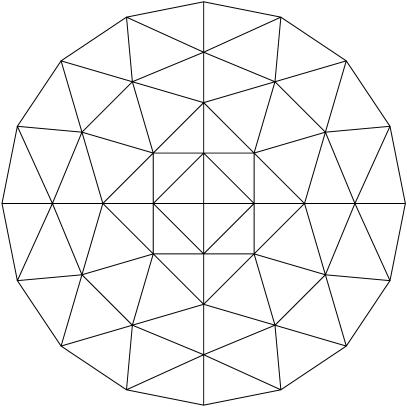
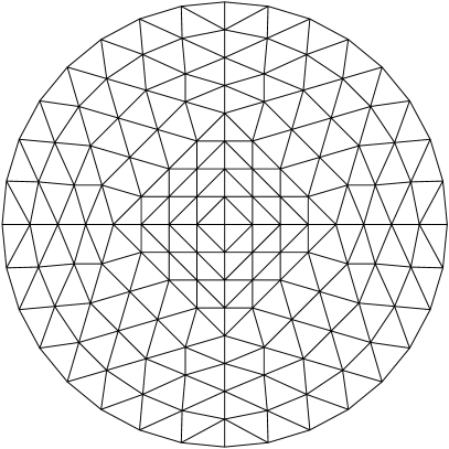
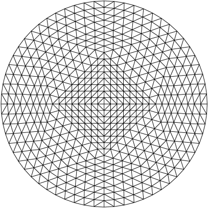
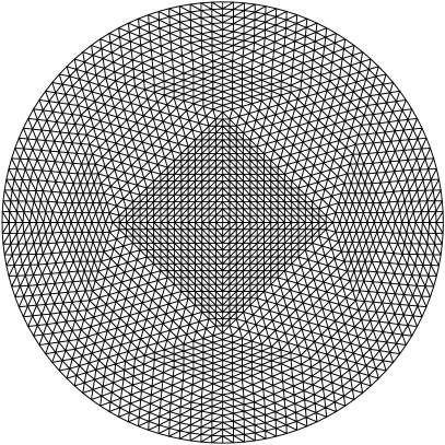
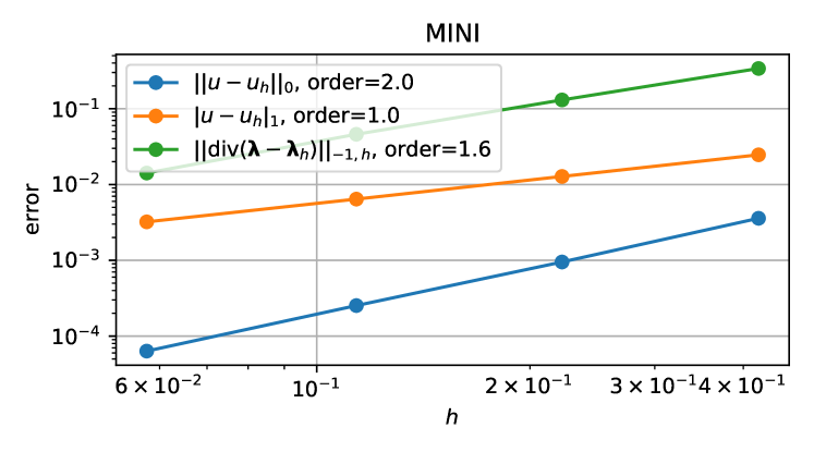
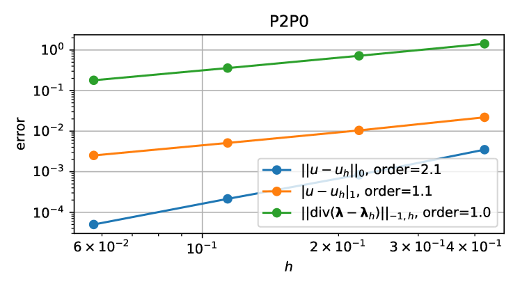
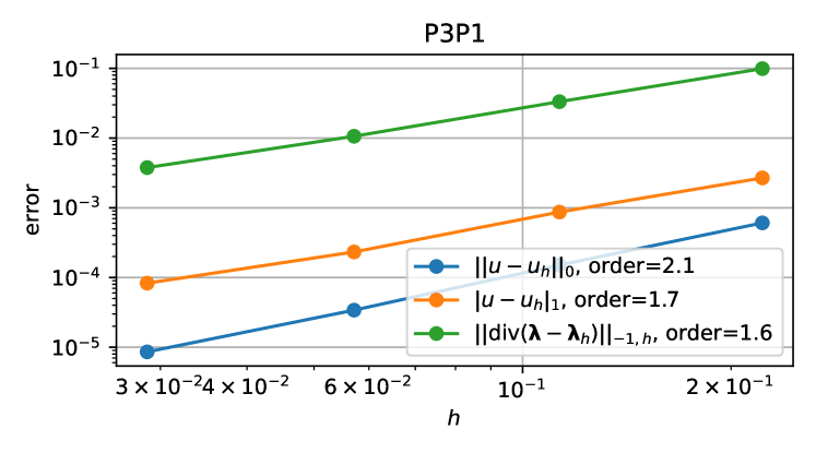
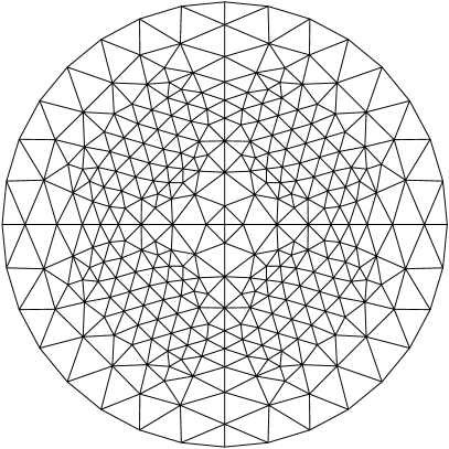
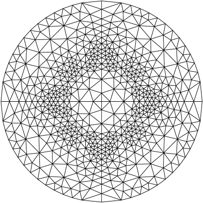
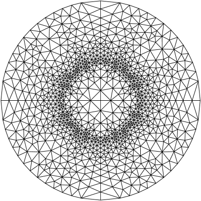
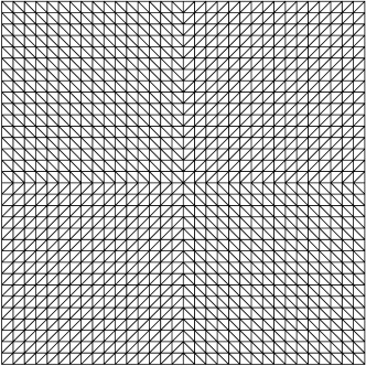
We first attempt to approximate an analytical solution on a circle using uniform mesh refinements; see Figure 1 for the sequence of meshes. For constant loading , the coincidence set is a smaller circle with the radius . The analytical solution reads when and is equal to the constant when . Substituting the above expression into the strong formulation (1a) we find also an analytical expression for the divergence of .
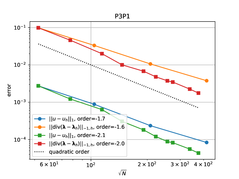
The error of the different components of the discrete norm are given in Figure 2 with , , , and in accordance to the suggestion in [17, Remark 3]. We observe that for the MINI and methods all components converge at least linearly whereas for method the seminorm of is approximately and the discrete norm of is approximately , i.e. less than the quadratic convergence order that interpolation estimates would imply for a completely smooth solution.
Next, our aim is to improve the convergence rate with respect to the total number of degrees-of-freedom using mesh adaptivity. We use an adaptive mesh sequence based on the a posteriori estimate of Section 5. An element-wise error estimator is given by
and we split if
The mesh is refined using the red-green-blue refinement strategy and Laplacian smoothing is applied on the refined mesh to improve its shape regularity. Some examples from the sequence of adaptive meshes are given in Figure 3. A comparison of the error between the uniform and adaptive mesh sequences is given in Figure 4. In particular, we observe that while the convergence rate of the error is ultimately dictated by the largest component of the discrete norm (i.e. ), there is a visible improvement in all of the components and, as a conclusion, the quadratic rate is recovered with respect to the number of degrees-of-freedom.
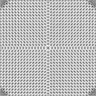
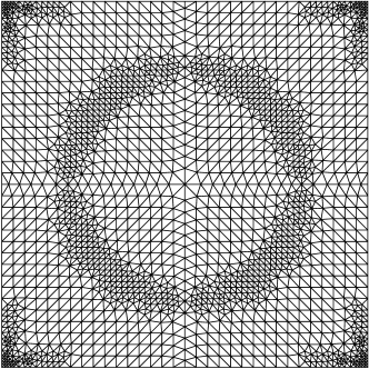
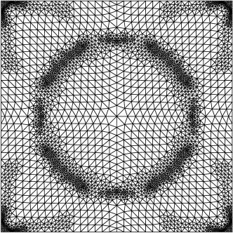
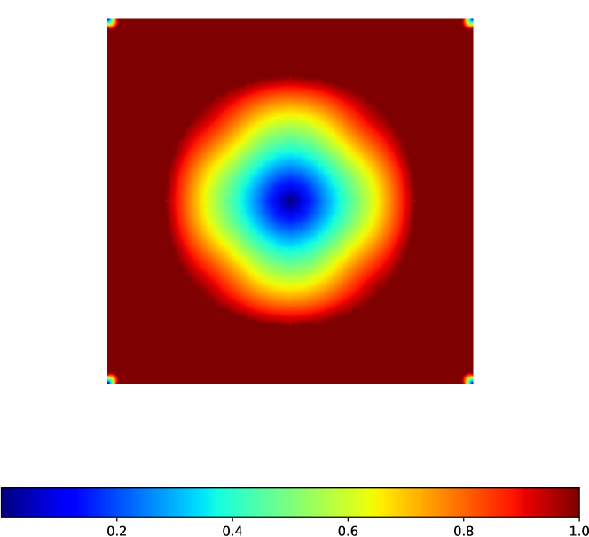
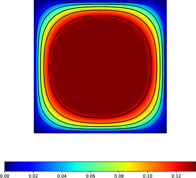
Finally, we consider an example in a square domain with , , , and no analytical solution; cf. [15, 23] for similar examples. Some meshes from the adaptive sequence and the total error estimators are given in Figure 5. The final discrete solution is depicted in Figure 6. As before, we observe the adaptive refinement focusing on the interfaces between the liquid and solid regions. Moreover, the estimators successfully locate and refine the so-called stagnating regions at corners of the square.
Remark 2.
We used a quadratic representation of the circle boundary in order to neglect the effect of inexact geometry representation.
Remark 3.
We found the following equivalent form of the estimator to be more robust against numerical tolerances in Algorithm 1:
Remark 4.
We consider methods only up to a linear Lagrange multiplier because for a higher order method, in general, when using Algorithm 1.
Acknowledgements
The numerical results were created using scikit-fem [13] which relies heavily on NumPy [16], SciPy [25] and Matplotlib [19]. The work was supported by the Academy of Finland (decisions 324611 and 338341).

References
- [1] N. J. Balmforth, I. A. Frigaard, and G. Ovarlez, Yielding to stress: recent developments in viscoplastic fluid mechanics, in Annual review of fluid mechanics. Vol. 46, vol. 46 of Annu. Rev. Fluid Mech., Annual Reviews, Palo Alto, CA, 2014, pp. 121–146.
- [2] D. Braess, Finite Elemente - Theorie, schnelle Löser und Anwendungen in der Elastizitätstheorie, Springer, 2013.
- [3] C. Carstensen, Clément interpolation and its role in adaptive finite element error control, in Partial differential equations and functional analysis, vol. 168 of Oper. Theory Adv. Appl., Birkhäuser, Basel, 2006, pp. 27–43.
- [4] C. Carstensen, B. D. Reddy, and M. Schedensack, A natural nonconforming FEM for the Bingham flow problem is quasi-optimal, Numerische Mathematik, 133 (2016), pp. 37–66.
- [5] K. L. Cascavita, J. Bleyer, X. Chateau, and A. Ern, Hybrid discretization methods with adaptive yield surface detection for Bingham pipe flows, Journal of Scientific Computing, 77 (2018), pp. 1424–1443.
- [6] P. Clément, Approximation by finite element functions using local regularization, RAIRO Analyse Numérique, 9 (1975), pp. 77–84.
- [7] G. Duvaut and J.-L. Lions, Inequalities in mechanics and physics, vol. 219 of Grundlehren der Mathematischen Wissenschaften, Springer-Verlag, Berlin-New York, 1976. Translated from the French by C. W. John.
- [8] R. S. Falk and B. Mercier, Error estimates for elasto-plastic problems, RAIRO Analyse Numérique, 11 (1977), pp. 135–144, 219.
- [9] M. Fuchs and G. Seregin, Variational methods for problems from plasticity theory and for generalized Newtonian fluids, vol. 1749 of Lecture Notes in Mathematics, Springer-Verlag, Berlin, 2000.
- [10] V. Girault and P.-A. Raviart, Finite element methods for Navier-Stokes equations, vol. 5 of Springer Series in Computational Mathematics, Springer-Verlag, Berlin, 1986. Theory and algorithms.
- [11] R. Glowinski, Sur l’approximation d’une inéquation variationnelle elliptique de type Bingham, ESAIM: Mathematical Modelling and Numerical Analysis - Modélisation Mathématique et Analyse Numérique, 10 (1976), pp. 13–30.
- [12] R. Glowinski, Numerical methods for nonlinear variational problems, Springer Series in Computational Physics, Springer-Verlag, New York, 1984.
- [13] T. Gustafsson and G. D. McBain, scikit-fem: A Python package for finite element assembly, Journal of Open Source Software, 5 (2020), p. 2369.
- [14] T. Gustafsson, R. Stenberg, and J. Videman, Mixed and stabilized finite element methods for the obstacle problem, SIAM Journal on Numerical Analysis, 55 (2017), pp. 2718–2744.
- [15] D. Hage, N. Klein, and F. T. Suttmeier, Adaptive finite elements for a certain class of variational inequalities of second kind, Calcolo, 48 (2011), pp. 293–305.
- [16] C. R. Harris, K. J. Millman, S. J. Van Der Walt, R. Gommers, P. Virtanen, D. Cournapeau, E. Wieser, J. Taylor, S. Berg, N. J. Smith, et al., Array programming with NumPy, Nature, 585 (2020), pp. 357–362.
- [17] J. W. He and R. Glowinski, Steady Bingham fluid flow in cylindrical pipes: a time dependent approach to the iterative solution, vol. 7, 2000, pp. 381–428. Numerical linear algebra methods for computational fluid flow problems.
- [18] R. R. Huilgol and M. Panizza, On the determination of the plug flow region in Bingham fluids through the application of variational inequalities, Journal of Non-Newtonian Fluid Mechanics, 58 (1995), pp. 207–217.
- [19] J. D. Hunter, Matplotlib: A 2d graphics environment, Computing in science & engineering, 9 (2007), pp. 90–95.
- [20] P. Mosolov and V. Miashikov, On stagnant flow regions of a viscous-plastic medium in pipes, Journal of Applied Mathematics and Mechanics, 30 (1966), pp. 841–854.
- [21] P. Mosolov and V. Miasnikov, On qualitative singularities of the flow of a viscoplastic medium in pipes, Journal of Applied Mathematics and Mechanics, 31 (1967), pp. 609–613.
- [22] N. Roquet and P. Saramito, An adaptive finite element method for Bingham fluid flows around a cylinder, Computer Methods in Applied Mechanics and Engineering, 192 (2003), pp. 3317–3341.
- [23] P. Saramito and N. Roquet, An adaptive finite element method for viscoplastic fluid flows in pipes, Computer Methods in Applied Mechanics and Engineering, 190 (2001), pp. 5391–5412.
- [24] R. Stenberg, A technique for analysing finite element methods for viscous incompressible flow, vol. 11, 1990, pp. 935–948. The Seventh International Conference on Finite Elements in Flow Problems (Huntsville, AL, 1989).
- [25] P. Virtanen, R. Gommers, T. E. Oliphant, M. Haberland, T. Reddy, D. Cournapeau, E. Burovski, P. Peterson, W. Weckesser, J. Bright, et al., SciPy 1.0: fundamental algorithms for scientific computing in Python, Nature methods, 17 (2020), pp. 261–272.