PyRelationAL: a python library for active learning research and development

Abstract

In constrained real-world scenarios, where it may be challenging or costly to generate data, disciplined methods for acquiring informative new data points are of fundamental importance for the efficient training of machine learning (ML) models. Active learning (AL) is a sub-field of ML focused on the development of methods to iteratively and economically acquire data through strategically querying new data points that are the most useful for a particular task. Here, we introduce PyRelationAL, an open source library for AL research. We describe a modular toolkit that is compatible with diverse ML frameworks (e.g. PyTorch, scikit-learn, TensorFlow, JAX). Furthermore, the library implements a wide range of published methods and provides API access to wide-ranging benchmark datasets and AL task configurations based on existing literature. The library is supplemented by an expansive set of tutorials, demos, and documentation to help users get started. PyRelationAL is maintained using modern software engineering practices — with an inclusive contributor code of conduct — to promote long term library quality and utilisation. PyRelationAL is available under a permissive Apache licence on PyPi and at https://github.com/RelationRx/pyrelational,

Keywords: active learning, bayesian optimization, open source software

1 Introduction

Machine learning (ML) methods, particularly those incorporating deep learning, play an increasing role in modern scientific research and broader society due to strong performance across tasks and domains. However, the success of such learning algorithms has often been fueled by large annotated datasets. Unfortunately, many important domains - including biology and medicine - operate in low data regimes, such that the amount of data available is relatively small compared to the rich and complex systems of interest. This problem can be largely attributed to the staggering cost and resources required to acquire and label a sufficient number of entities for effective learning (Smith et al., 2018; Abdelwahab and Busso, 2019; Hoi et al., 2006).

Active learning (AL), or query learning (Settles, 2012), is a machine learning paradigm where the aim is to develop methods, or strategies, to improve model performance in a data-efficient manner. Intuitively, an AL strategy seeks to sample data points economically such that the resulting model performs as well as possible under budget constraints. This is typically achieved via an interactive process whereby the model can sequentially query samples based on current knowledge and expected information gain. Many notions in AL can be related to research in Bayesian optimization (Brochu et al., 2010) and reinforcement learning (Sutton and Barto, 2018), as all aim to strategically explore some space while optimising a given criterion. Recently, there has been renewed interest in AL to address various real-world applications (Ren et al., 2021; Zhan et al., 2021). Notably, applications to medicine and drug research have been growing in number, in both academic and industrial settings (Smith et al., 2018; Abdelwahab and Busso, 2019; Hie et al., 2020; Bertin et al., 2022; Mehrjou et al., 2021).

Here, we introduce PyRelationAL, an open source Python library for the rapid, reliable and reproducible construction of AL pipelines and strategies. The design is modular and allows easy implementation of AL strategies within a consistent framework. PyRelationAL enables the reproduction of existing research, the application to new domains, and the design of new methods. We include a plethora of published methods as part of PyRelationAL to help users get started and facilitate development around popular state of the art approaches. Historically, open source ML libraries that have played a major role in the fast paced advancement of ML have all adopted a practical, researcher-first ethos coupled with flexible design principles (Paszke et al., 2019; Chollet et al., 2015; Bradbury et al., 2018; Heek et al., 2020; Tran et al., 2017; Gardner et al., 2018; Phan et al., 2019). By following these same principles, our hope is that PyRelationAL will have a similar transformative impact on AL research.

2 Framework overview

To accommodate for the research and development of bespoke AL pipelines and strategies, PyRelationAL prescribes a modular framework devised of 5 core components that together facilitate a generic active learning pipeline. For a primer in AL we refer readers to Appendix A or our tutorials online. We follow the terminology introduced in (Settles, 2012).

• Data Manager: The DataManager stores the dataset, keeps track of annotated and unannotated data subsets, handles the creation of data loaders for each subset, and interacts with the oracle to update data annotations.

• Model Manager: The ModelManager wraps the learning algorithm and organises its training and evaluation. This abstraction supports the implementation of models written in diverse frameworks to interface with other PyRelationAL modules.

• Strategy: The Strategy carries the responsibility of suggesting unlabelled observations to an oracle for annotation based on their perceived informativeness. Users can define active learning algorithms via the pyrelational.Strategy.__call__() method. We have implemented a variety of seminal informativeness measures and strategies from AL literature for users to build upon, see Appendix B for details.

• Oracle: In PyRelationAL the Oracle implements interfaces to entities which provide annotations given input observations from the dataset. With this one may interface PyRelationAL to various existing annotation tools such as Label Studio (Tkachenko et al., 2020-2022), bespoke labelling tools, and X-in-the-loop pipelines.

• Pipeline: The Pipeline arbitrates the active learning cycle and the communication between its DataManager, ModelManager, Strategy, Oracle components. It also logs various data for the evaluation of different active learning strategies such as the performance of the model at each iteration.

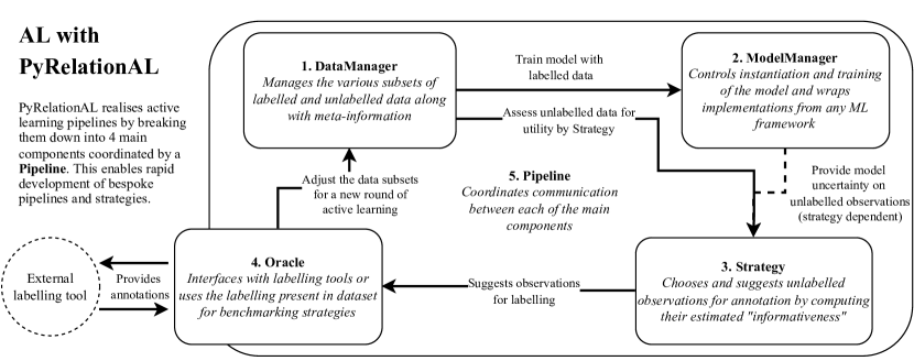
Figure 1: Diagram of PyrelationAL’s modular approach to constructing full active learning pipelines.

This framework allows users to focus on different facets of the active learning cycle whether it be dataset processing and management, machine learning model design, the active learning strategy, or the flow of the pipeline whilst under the assurance that other components adhere to a consistent API. Using a ModelManager abstraction also enables user flexibility in their choice of ML framework, a feature which most current AL libraries lack (see Table 7 in Appendix F). To get users started we have created a number of annotated examples and online tutorials of active learning strategies based on existing methods, coupled with various custom implementations of models using SciKit-Learn, PyTorch, GPyTorch. PyRelationAL also provides model managers for ensembling (Lakshminarayanan et al., 2017; Cohn et al., 1994; Seung et al., 1992) and Monte-Carlo dropout (Gal and Ghahramani, 2016), which are heuristics commonly used to approximate model uncertainties. In Appendix C, interested readers can find additional information about the implementation of novel active learning strategies, and a full coding example with a custom dataset and ML model.

Benchmark datasets and tasks for AL

A core part of ML research and development is the translation of theory to practice typically in the form of evaluating a proposed method empirically against a range of established or challenging benchmark datasets and tasks. However, despite a multitude of papers, surveys, and other libraries for AL there is no established set of datasets evaluating AL strategies (see Appendix F). This has made the horizontal assessment of existing and novel AL strategies on common grounds particularly challenging as noted in recent reviews of (Zhan et al., 2021; Yang and Loog, 2018; Wu, 2019).

To help alleviate this issue we have collected a variety of real-world and synthetic datasets (see Table 2 in Appendix D) for both classification and regression tasks as used in AL literature and make these available through PyRelationAL. Each dataset can be downloaded in preprocessed format as a PyTorch Dataset through our API. Additionally, for each dataset we provide annotation scenarios which challenge active learning strategies on the different circumstances of the initial labellings and train-test distributions, which can also be changed to bespoke settings by the user. We have found or contacted each of the original authors to ensure a proper licence is attributed to the datasets and tasks to help users abide by ethical usage terms and proper attribution. This is a novel contribution to the AL infrastructure landscape that will help users benchmark their strategies, and over the long term lead to better characterisation of the strengths and limitations of AL methods. More information on datasets and tasks is available in Appendix D along with a comparative analysis using a selection of the included AL strategies in Appendix E.

3 Maintaining PyRelationAL

We adopt modern open source software engineering practices in order to promote robustness and reliability of the package whilst maintaining an open policy towards contributions over the long term vision we have for the project.

Open sourcing, package indexing, and contributing

PyRelationAL is made available open source under a permissive Apache 2.0 licence with stable releases made on the Python Package Index (PyPI) for easy installation. To introduce new users to the package we created an extensive set of examples, tutorials, and supplementary materials linked through the main README including developer setups for contributors. We follow an inclusive code of conduct for contributors and users to facilitate fair treatment and guidelines for contributing. Furthermore, a contributors guide is provided describing the expected workflows, testing, and code quality expectations for pull requests into the package.

Documentation

All modules are accompanied by restructured text (ResT) docstrings and comments to maintain documentation of the library. This approach maintains an up to date reference of the API, which is compiled and rendered via Sphinx to be hosted on Read the Docs for every update accepted into the main branch.

Code quality, testing and continuous integration

To ensure consistent code quality throughout the package, we ensure that source code is PEP 8 compliant via a linter that is checked automatically before a pull request can be approved. We make pre-commit hooks available that can format the code using tools, such as the Black package. All important modules and classes are extensively tested through unit tests to ensure consistent behaviour. Code coverage reports are available on the repository as a measure of the health of the package. A continuous integration setup ensures that any update to the code base is tested across different environments and can be installed reliably. Furthermore, we use the mypy package for type checks to enforce consistency and ensure quality across the library. As an added benefit, the type hints facilitate the interfacing of PyRelationAL with other libraries.

Appendix A. Active learning primer.

Notations

Let $\mathcal{X}$ denote a state space whereby each element $x\in\mathcal{X}$ can be associated to a label $y\in\mathcal{Y}$. We further denote by $\mathcal{F}$ the space of functions mapping $f:\mathcal{X}\mapsto\mathcal{Y}$. For a given ML architecture, we denote by $\mathcal{F}_{\Theta}\subset\mathcal{F}$ the subset of function mappings having this architecture and parameters in $\Theta$, which is defined by the model’s hyperparameters. The world, $\mathcal{W}\subset\mathcal{X}\times\mathcal{Y}$, is defined by a canonical mapping $\omega\in\mathcal{F}$ that associates to each state a unique label. We assume we have initially access to a set of observations $\mathcal{L}_{0}\subset\mathcal{W}$ from the world. We denote by $\mathcal{U}_{0}\subset\mathcal{X}$ the set of elements that are not observed in $\mathcal{L}_{0}$. The task we are faced with is to approximate the canonical mapping function $\omega$ from a subset of observations of $\mathcal{W}$, i.e. find $f\in\mathcal{F}$ such that $\forall x\in\mathcal{X},f(x)\approx\omega(x)$.

Supervised learning

To address this task in the supervised ML paradigm, one first defines a function space $\mathcal{F}_{\Theta}$, through various inductive biases and hyperparameter tuning. Then one searches for a function $f_{\hat{\theta}}\in\mathcal{F}_{\Theta}$, with parameters $\hat{\theta}\in\Theta$, that best approximate $\omega$.

Active learning

In the AL paradigm, the function space $\mathcal{F}_{\Theta}$ is largely assumed to be fixed. However, the practitioner can iteratively increase the size of the dataset by strategically querying the labels for some unlabelled elements in $\mathcal{X}$. At the $k^{\textnormal{th}}$ iteration, we denote by $\mathcal{L}_{k}$ the dataset and by $\mathcal{U}_{k}$ the set of unlabelled elements. The goal of an AL strategy is to identify a query set $\mathcal{Q}_{k}\subset\mathcal{U}_{k}$ that carries the most information for approximating $\omega$. In other words, the AL practitioner looks to add new observations strategically to identify a smaller space $\mathcal{F}_{\Theta,k+1}$ of functions that are compatible with $\mathcal{L}_{k+1}=\mathcal{L}_{k}\bigcup\big{\{}\left(q,\omega(q)\right),\,q\in\mathcal{Q}_{k}\big{\}}$, whereby the queries’ labels are provided by an oracle, e.g. human annotators or laboratory experiments. We then update $\mathcal{U}_{k+1}=\mathcal{U}_{k}\setminus\mathcal{Q}_{k}$ for the next iteration. Access to the oracle is costly, thus AL typically operates under a budget constraint limiting the total number of possible queries.

The general framing described above is sometimes referred to as pool-based AL (Settles, 2012), where $\mathcal{U}_{k}$ defines the pool at the $k^{\textnormal{th}}$ iteration. This is arguably the most common framing of the AL problem. However, there exist variations whereby at each iteration $\mathcal{U}_{k}$ is not a finite set but either a generative process or a stream of unlabelled observations. These are known as membership query and stream based AL, respectively (Settles, 2012). All framings share the same core problem: identifying unlabelled observations that are most informative to improving our solution to the task. In our exposition, we will principally focus on pool-based AL unless otherwise specified.

A critical question underpinning AL is how to measure the informativeness of each state in $\mathcal{X}$. A number of heuristics have been proposed in the past which can broadly be split into two categories: 1.) uncertainty-based category and 2.) diversity-based category. These are not mutually exclusive as the two notions can be combined to positive effect (Settles, 2012; Brinker, 2003; Monarch, 2021). The former relies on some measure of uncertainties of the predictions obtained from the set of functions $\mathcal{F}_{\Theta,k}$ at each iteration. In practice, $\mathcal{F}_{\Theta,k}$ can be defined intrinsically by the class of ML models (e.g. Gaussian processes or Bayesian neural networks) or a subset of it can be obtained using heuristics such as ensembling (Lakshminarayanan et al., 2017; Cohn et al., 1994; Seung et al., 1992) or Bayesian inference approximation methods like MCDropout (Gal and Ghahramani, 2016). Various informativeness scores can be computed from the uncertainty estimates (see Table 1) and used to select the query set $\mathcal{Q}_{k}$. In contrast, diversity-based heuristics rely on a distance measure $d:\mathcal{X}\times\mathcal{X}\mapsto\mathbb{R}_{+}$, which can depend on $\mathcal{F}_{\Theta,k}$, to score states in $\mathcal{U}_{k}$ with respect to elements in $\mathcal{L}_{k}$. The choice of informativeness measure is an important challenge of AL as well as the choice of query selection strategy from the informativeness scores.

A standard approach to select $\mathcal{Q}_{k}$ is to greedily pick the highest scoring elements such that

$$Q_{k}=\operatorname*{argmax}_{\begin{subarray}{c}\mathcal{Q}\subset\mathcal{U}_{k}\\ |\mathcal{Q}|=m_{k}\end{subarray}}\sum_{q\in\mathcal{Q}}I(q),$$

where $I:\mathcal{X}\mapsto\mathbb{R}$ denotes an information measure that typically would depend on $\mathcal{F}_{\Theta,k}$, and $m_{k}$ corresponds to the number of queries desired at round $k$. However, for $m_{k}>1$, this selection strategy can lead to a redundant query set as each query therein is selected independently of the others. The sub-field of batch active learning is concerned with this issue and developing strategies to ensure some notion of diversity in the query (Settles, 2012; Brinker, 2003; Guo and Schuurmans, 2007). For instance, BatchBALD (Kirsch et al., 2019) relies on minimising the mutual information between pairs of queries in $\mathcal{Q}_{k}$.

Appendix B. Informativeness measures.

In this section, we provide more details about each type of informativeness measure discussed in Appendix A and describe some of the specific scores mentioned in Table 1.

Table 1: List of informativeness measures implemented in PyRelationAL currently. The task column indicates whether the corresponding informativeness measure is defined for classification, regression, or is agnostic (Any) to the ML task being performed.

Name	Task	Ref.
Entropy	Classification	(Dagan and Engelson, 1995; Settles, 2012)
Least confidence	Classification/Regression	(Lewis and Catlett, 1994; Settles, 2012)
Margin confidence	Classification	(Scheffer et al., 2001; Settles, 2012)
Ratio confidence	Classification	(Scheffer et al., 2001)
Greedy score	Regression	(De Ath et al., 2021)
Upper confidence bound	Regression	(De Ath et al., 2021)
Expected improvement	Regression	(De Ath et al., 2021)
Bayesian active learning by disagreement	Classification/Regression	(Houlsby et al., 2011b)
Thompson sampling	Regression	(Russo et al., 2018)
Representative sampling	Any	(Nguyen and Smeulders, 2004)
Relative distance	Any	(Dasgupta and Hsu, 2008)

Uncertainty-based informativeness scores

As discussed in Appendix A, a large number of informativeness measures rely on some estimate of prediction uncertainties. The underlying rationale is that regions of the world are highly uncertain because they are poorly represented in the training data. Improving coverage through sampling uncertain data regions can enable significant global performance gains. While this makes intuitive sense, it ignores subtleties about the nature of uncertainties which can be decomposed in epistemic and aleatoric components (Der Kiureghian and Ditlevsen, 2009). The former is understood as coming from modelling errors while the latter is inherent to the world, corresponding to natural variations or measurement noise. Aleatoric uncertainties are irreducible and, in practice, it is extremely difficult to tease out the two uncertainty components from each other. This means that uncertainty-based informativeness scores can overestimate the information gain that a sample would provide. In the following, we detail a few of the scores that fall under this category.

Entropy

is a well-established notion in information theory that quantifies the uncertainty of a probability distribution over possible outcomes (Shannon, 1948). It is used as an informativeness measure for classification tasks where the probability distribution is defined over the finite set of labels $\mathcal{Y}$. Specifically, it is defined as

$$I(x)=-\sum_{y\in\mathcal{Y}}p_{\mathcal{F}_{\theta,k}}\left(y|x\right)\log\left(p_{\mathcal{F}_{\theta,k}}\left(y|x\right)\right).$$

Least confidence

can be used both for regression and classification tasks, although the score is defined differently for each task. In regression tasks, we have

$$I(x)=\textnormal{Var}_{\mathcal{F}_{\theta,k}}\left[Y|x\right],$$

where Y denotes a random variable in $\mathcal{Y}$. Hence, to each sample $x$ it associates the variance across the predictions from the set of functions $\mathcal{F}_{\theta,k}$.

In classification tasks, the least confidence score is defined as

$$I(x)=1-\max_{y\in\mathcal{Y}}\,p_{\mathcal{F}_{\theta,k}}\left(y|x\right).$$

Margin confidence

was introduced for classification tasks and measures uncertainty as the difference between the highest and second highest probabilities associated to labels in $\mathcal{Y}$ derived from our predictions on a given sample. The smaller that difference, the higher the uncertainty. In equation, this gives

$$y_{0} =\operatorname*{argmax}_{y\in\mathcal{Y}}p_{\mathcal{F}_{\theta,k}}\left(y|x\right),$$

$$y_{1} =\operatorname*{argmax}_{y\in\mathcal{Y}\setminus\{y_{0}\}}p_{\mathcal{F}_{\theta,k}}\left(y|x\right),$$

$$I(x) =1-\left(p_{\mathcal{F}_{\theta,k}}\left(y_{0}|x\right)-p_{\mathcal{F}_{\theta,k}}\left(y_{1}|x\right)\right).$$

Ratio confidence

is a score similar to margin confidence, the only difference comes from the fact that the uncertainty is expressed as a ratio between the two probabilities

$$y_{0} =\operatorname*{argmax}_{y\in\mathcal{Y}}p_{\mathcal{F}_{\theta,k}}\left(y|x\right),$$

$$y_{1} =\operatorname*{argmax}_{y\in\mathcal{Y}\setminus\{y_{0}\}}p_{\mathcal{F}_{\theta,k}}\left(y|x\right),$$

$$I(x) =\frac{p_{\mathcal{F}_{\theta,k}}\left(y_{1}|x\right)}{p_{\mathcal{F}_{\theta,k}}\left(y_{0}|x\right)}.$$

Greedy score

This is a simple score used for regression tasks where greater values in $\mathcal{Y}$ are of higher interest. For instance, we would be more interested in reliably identifying highly synergistic pairs of drugs. The score is defined as

$$I(x)=\textnormal{E}_{\mathcal{F}_{\theta,k}}\left[Y|x\right].$$

Upper confidence bound

UCB comes from the reinforcement learning (RL) literature and corresponds to a trade-off, controlled by an hyperparameter $\lambda$, between the greedy score and the least confidence score. It is formally defined as

$$I(x)=\textnormal{E}_{\mathcal{F}_{\theta,k}}\left[Y|x\right]+\lambda\sqrt{\textnormal{Var}_{\mathcal{F}_{\theta,k}}\left[Y|x\right]},$$

where Y denotes a random variable in $\mathcal{Y}$.

Similarly to the greedy score, it is defined for continuous label values and assumes that greater values, known as rewards in RL, are more relevant to the problem.

Diversity-based informativeness scores

Rather than rely on some estimate of uncertainties, diversity-based scores aim to increase the diversity of the training set, querying samples that are far from the current labelled set according to a selected distance metric. Methods can differ on the choice of distance metric and on the space where distances are computed. The feature space is often used but can have some limitations due to noisy or redundant features or suffer from the curse of dimensionality in high-dimensional space. As such, researchers have proposed to compute distances in lower dimensional spaces either obtained from dimensionality reduction techniques or from intermediary latent spaces derived from a trained model. We discuss below two generic types of approaches that are built-in PyRelationAL.

Relative distance sampling

computes the minimum distance from an unlabelled sample to the labelled samples

$$I(x)=\min_{l\in\mathcal{L}}d\left(\phi(x),\phi(l)\right),$$

where $\phi:\mathcal{X}\mapsto\mathbb{R}^{m}$ an embedding function projecting samples into a latent space and $d:\mathbb{R}^{m}\times\mathbb{R}^{m}\mapsto\mathbb{R}_{+}$ represents the chosen distance metric in the latent space. Note that $\phi$ is simply the identity function when computing distances in the ambient space. The coreset approach, as defined in Mehrjou et al. (2021), would be classified in this category in PyRelationAL, where the latent space representation of a point is defined by the associated penultimate activations in a neural network.

Representative sampling

does not explicitly define an informativeness scores. Instead, it groups the current unlabelled set into a fixed number of clusters and selects representative samples from each cluster to form the query set. Note that this can be quite expensive to compute when the unlabelled set is large as it requires all-to-all pairwise distances, and can benefit from extracting first a subset of the unlabelled set based on some other criteria.

Appendix C. Full coding example with custom modules.

In this section, we will walk through a full coding example of a pool based active learning scenario using a bespoke dataset, model, and strategy. In doing so we will go over the use and custom extension of the DataManager, ModelManager, Strategy, Oracle, and Pipeline components as detailed in Section 2. For this exercise, we will use the diabetes dataset from Scikit-Learn (Pedregosa et al., 2011) which contains data for 442 patients, each described by 10 features (such as age, sex, and BMI) and associated with a scalar score quantifying the disease’s progression, or stage. The distribution of these scores is shown in Figure 3.

⬇

import torch

from sklearn.datasets import load_diabetes

from torch.utils.data import Dataset

\parclass DiabetesDataset(Dataset):

def __init__(self):

# Load the diabetes dataset

diabetes_X, diabetes_y = load_diabetes(

return_X_y=True

)

self.x = torch.FloatTensor(diabetes_X)

self.y = torch.FloatTensor(diabetes_y)

\pardef __len__(self):

return self.x.shape[0]

\pardef __getitem__(self, idx):

return self.x[idx], self.y[idx]

Creating a PyTorch dataset for a regression task using the Diabetes dataset from scikit-learn.

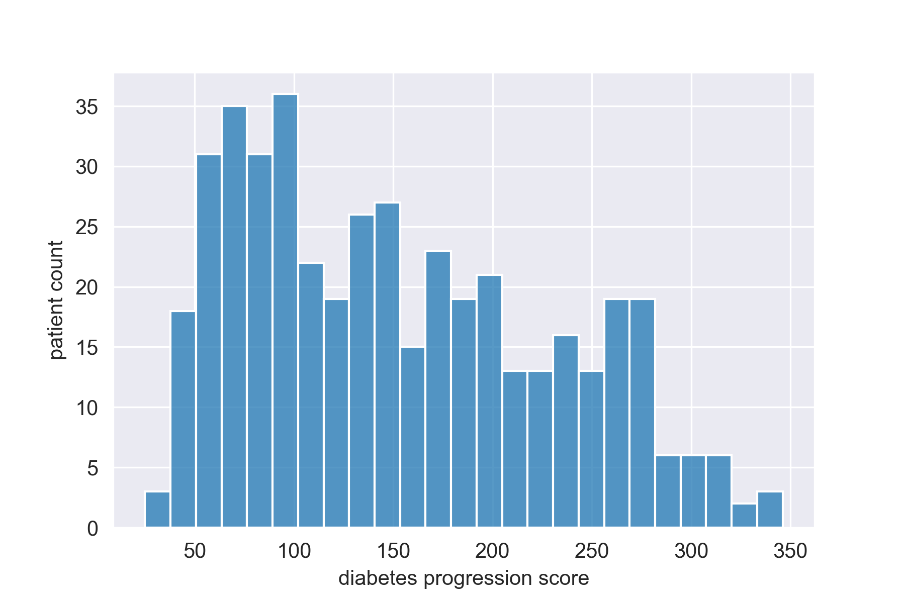
Figure 3: Distribution of the diabetes progression score in the dataset considered.

We then wrap our PyTorch Dataset object within a PyRelationAL DataManager (see Listings 4), randomly splitting the data into train, validation, and test sets (lines 9-12) and taking a portion of the train set as our initial labelled set (lines 16-21).

⬇

from pyrelational.data_managers import DataManager

\pardef get_data_manager(

batch_size=10,

hit_ratio_at=5,

labelled_size = 100,

):

ds = DiabetesDataset()

train_ds, valid_ds, test_ds = torch.utils.data.random_split(

ds,

[400, 22, 20],

)

train_indices = train_ds.indices

valid_indices = valid_ds.indices

test_indices = test_ds.indices

labelled_indices = (

train_indices[:labelled_size]

if not labelled_size is None

else None

)

\parreturn DataManager(

ds,

train_indices=train_indices,

validation_indices=valid_indices,

test_indices=test_indices,

labelled_indices=labelled_indices,

loader_batch_size=batch_size,

hit_ratio_at=hit_ratio_at,

)

Defining a PyRelationAL data manager for the dataset.

Let us define a simple multi-layer perceptron model (see Listings 5) to predict diabetes progression based on the input features describing each patient.

⬇

import torch

import torch.nn as nn

import torch.nn.functional as F

\parclass DiabetesRegression(nn.Module):

def __init__(self, dropout=0):

super(DiabetesRegression, self).__init__()

self.layer_1 = nn.Linear(10, 5)

self.layer_2 = nn.Linear(5, 1)

self.elu = nn.ELU()

self.dropout = nn.Dropout(dropout)

\pardef forward(self, x):

x = self.dropout(self.elu(self.layer_1(x)))

x = self.dropout(self.layer_2(x))

return x

A simple MLP regression model implemented in PyTorch.

We define a PyRelationAL ModelManager to wrap around the PyTorch model in Listings 6, by overriding the train() (lines 19-35) and test() (lines 37-47) methods. As the neural network provides point estimates, we will obtain prediction uncertainty estimates through Bayesian inference approximation. To do so we will use ensembling with PyRelationAL’s EnsembleModelManager which extends the ModelManager to add this functionality. This class handles instantiation of an ensemble of DiabetesRegression models of whose number is governed by the n_estimators argument (line 10).

⬇

import torch

import torch.nn as nn

from pyrelational.model_managers import EnsembleModelManager

\parclass TorchEnsembleWrapper(EnsembleModelManager):

def __init__(self,

model_class,

model_config,

trainer_config,

n_estimators= 5,

):

super(TorchEnsembleWrapper, self).__init__(

model_class,

model_config,

trainer_config,

n_estimators,

)

\pardef train(self, train_loader, val_loader=None):

criterion = nn.MSELoss()

self._current_model = []

for _ in range(self.n_estimators):

model = self._init_model()

optimizer = torch.optim.Adam(

model.parameters(),

lr=self.trainer_config["lr"]

)

for _ in range(self.trainer_config["epochs"]):

for x, y in train_loader:

optimizer.zero_grad()

out = model(x)

loss = criterion(out, y)

loss.backward()

optimizer.step()

self._current_model.append(model)

\pardef test(self, loader):

with torch.no_grad():

tst_loss, cnt = 0, 0

for model in self._current_model:

model.eval()

for x, y in loader:

tst_loss += torch.square(

model(x) - y

).sum()

cnt += x.size(0)

return {"test_loss": tst_loss/cnt}

Defining a PyTorch model wrapper for PyRelationAL with additional ensembling functionality to obtain prediction uncertainty estimates.

For this exercise we will create implement an $\epsilon$-greedy strategy (see Listings 7). Borrowed from reinforcement learning literature, this strategy interpolates between a random strategy, that selects patients for labelling at random, and a greedy strategy, that selects patients whose diabetes is predicted to be most advanced, and who might be in need of more care. The Strategy functionality is implemented by overriding the __call__() method which return indices to dataset observations which should be annotated. When utilised within a Pipeline, the arguments of the __call__() can pattern match to attributes of the pipeline. More details are given below with the Pipeline.

⬇

import torch

import numpy as np

from pyrelational.informativeness import (

regression_mean_prediction,

)

from pyrelational.strategies.abstract_strategy import (

Strategy,

)

\parclass EpsilonGreedyStrategy(Strategy):

def __init__(self, eps=0.05):

super(EpsilonGreedyStrategy, self).__init__()

assert 0 <= eps <= 1, "epsilon should be a float between 0 and 1"

self.eps = eps

\pardef __call__(self, num_annotate, data_manager, model_manager):

num_annotate = min(num_annotate, len(data_manager.u_indices))

output = self.train_and_infer(data_manager, model_manager)

scores = regression_mean_prediction(x=output, axis=0).squeeze()

ixs = torch.argsort(scores, descending=True).tolist()

greedy_annotate = int((1-self.eps)*num_annotate)

ixs = [data_manager.u_indices[i] \ for i in ixs[: greedy_annotate]]

remaining_u_indices = list(

set(data_manager.u_indices) - set(ixs)

)

random_annotate = np.random.choice(

remaining_u_indices,

num_annotate-greedy_annotate,

replace=False,

)

return ixs + random_annotate.tolist()

Implements an $\epsilon$-greedy strategy, whereby a percentage of the samples to annotate are selected randomly while the remaining are selected greedily.

With the definition of a DataManager, ModelManager, and Strategy, the remaining tasks are to complete the active learning cycle with an Oracle and Pipeline (see Listings 8). In this exercise, we will use the BenchmarkOracle (Line 14), which assumes all of the data in the DataManager is annotated and is primarily intended for benchmarking various strategies. As outlined in Section 2, the Pipeline is a composition of the DataManager, ModelManager, Strategy, and Oracle as in lines 15-20. It facilitates the expected communication between them and acts as an interface to the active learning cycle. Once instantiated we can ask the pipeline to use the components to provide indices of 25 unlabelled observations which are deemed most informative by the strategy in Line 23. With these indices we can query the oracle for labels and update the dataset in Line 24. Finally, as a convenience function, Line 27 continually runs the active learning cycle until there are no unlabelled observations left in the dataset.

⬇

from pyrelational.oracles import BenchmarkOracle

from pyrelational.pipeline import Pipeline

\par# A Pipeline is a composition of DataManager,

# ModelManager, Strategy, and Oracle objects

data_manager = get_data_manager()

model_manager = TorchEnsembleWrapper(

DiabetesRegression,

{"dropout": 0.12},

{"epochs":100, "lr":3e-4},

n_estimators=10,

)

strategy = EpsilonGreedyStrategy(eps=0.05)

oracle = BenchmarkOracle()

pipeline = Pipeline(

data_manager = data_manager,

model_manager = model_manager,

strategy = strategy,

oracle = oracle,

)

\par# New data to be annotated, followed by an update of the data_manager and model

to_annotate = pipeline.step(num_annotate=25)

pipeline.query(indices=to_annotate)

\par# Annotating data step by step until the trainset is fully annotated

pipeline.run(num_annotate=25)

Integrating each of the custom data manager, ensemble of models, and strategy into a pipeline along with an oracle for benchmarking strategies. After a pipeline is instantiated we may iterate on the active learning cycle.

Appendix D. Benchmark datasets and AL tasks.

A core part of ML research and development is the translation of theory to practice typically in the form of evaluating a proposed method empirically against a range of established or challenging benchmark datasets and tasks. The practice of empirically evaluating on established datasets and tasks has become so ubiquitous that all major ML frameworks such as PyTorch, TensorFlow, SciKit-Learn come with interfaces for downloading common benchmarks. The rapid progress of ML research in images, text, and graphs can be attributed at least partially to easy access to pre-processed benchmark datasets (Deng et al., 2009; Wang et al., 2019; Hu et al., 2020; Huang et al., 2021).

Table 2: Selection of datasets made available in the PyRelationAL library along with information on whether the ML task is a classification or regression, whether it is real-world or synthetic dataset, and the raw source of our implementation or the paper from which we constructed the dataset if it was not available publicly. We also give the licence of each dataset curated and extend our permissive Apache 2.0 licence (see section 3) to synthetic datasets generated with our code as well as the task configurations. Our selection was strongly based on their prior reference in related AL literature.

Name	ML Task	Type	Source	Use in AL literature	Licence
CreditCard	Classification	Real	(Pozzolo et al., 2015)	(Konyushkova et al., 2017)	DbCL 1.0
StriatumMini	Classification	Real	(Lucchi et al., 2013, 2012; Konyushkova et al., 2017)	(Konyushkova et al., 2017, 2015)	GPLv3
Breast	Classification	Real	(Dua and Graff, 2017)	(Houlsby et al., 2011a; Yang and Loog, 2018; Zhan et al., 2021)	CC BY 4.0
Glass	Classification	Real	(Dua and Graff, 2017)	(Cai et al., 2013; Du et al., 2017; Zhan et al., 2021)	CC BY 4.0
Parkinsons	Classification	Real	(Little et al., 2007; Dua and Graff, 2017)	(Xiong et al., 2014; Yang and Loog, 2018; Zhan et al., 2021)	CC BY 4.0
SynthClass1	Classification	Synthetic	(Yang and Loog, 2018)	(Yang and Loog, 2018)	Apache 2.0
SynthClass2	Classification	Synthetic	(Huang et al., 2015)	(Huang et al., 2015; Yang and Loog, 2018)	Apache 2.0
GaussianClouds	Classification	Synthetic	(Konyushkova et al., 2017)	(Konyushkova et al., 2017; Yang and Loog, 2018)	Apache 2.0
Checkerboard2x2	Classification	Synthetic	(Konyushkova et al., 2017)	(Konyushkova et al., 2017)	Apache 2.0
Checkerboard4x4	Classification	Synthetic	(Konyushkova et al., 2017)	(Konyushkova et al., 2017)	Apache 2.0
Diabetes	Regression	Real	(Efron et al., 2004; Dua and Graff, 2017)	(Houlsby et al., 2011a; Zhan et al., 2021)	CC BY 4.0
Concrete	Regression	Real	(Yeh, 1998; Dua and Graff, 2017)	(Wu, 2019)	CC BY 4.0
Energy	Regression	Real	(Tsanas and Xifara, 2012; Dua and Graff, 2017)	(Pinsler et al., 2019)	CC BY 4.0
Power	Regression	Real	(Tüfekci, 2014; Dua and Graff, 2017)	(Pinsler et al., 2019; Wu, 2019)	CC BY 4.0
Airfoil	Regression	Real	(Dua and Graff, 2017)	(Wu, 2019)	CC BY 4.0
WineQuality	Regression	Real	(Cortez et al., 2009; Dua and Graff, 2017)	(Wu, 2019)	CC BY 4.0
Yacht	Regression	Real	(Dua and Graff, 2017)	(Pinsler et al., 2019; Wu, 2019)	CC BY 4.0

However, despite a multitude of papers, surveys, and other libraries for AL methods there is no established set of datasets evaluating AL strategies. To further complicate matters the same datasets can be processed to pose different AL tasks such as cold and warm starts as described in Konyushkova et al. (2017) and Yang and Loog (2018) to provide different challenges to strategies. In other words, a benchmark for AL has to be considered from the characteristics of the dataset and the circumstances of the initial labelling.

Due to these challenges, AL papers have a tendency to test and apply proposed methods using different splits of the same datasets with little overlap agreement across papers — as noted in several reviews (Zhan et al., 2021; Yang and Loog, 2018; Wu, 2019). This makes it difficult to assess strategies horizontally across a range of common datasets and identify regimes under which a given strategy shows success or failure. This issue is exacerbated by publication bias which favours the reporting of positive results — as noted in Settles (Settles, 2012). To help alleviate this issue we have collected a variety of datasets for both classification and regression tasks as used in AL literature and make these available through PyRelationAL, see Table 2. The datasets are either real world datasets or synthetic datasets taken from seminal AL literature (Konyushkova et al., 2017; Pozzolo et al., 2015; Zhan et al., 2021; Yang and Loog, 2018; Wu, 2019; Pinsler et al., 2019). The synthetic datasets were typically devised to pose challenges to specific strategies. Another selection criteria was their permissive licensing, such as the Creative Commons Attribution 4.0 International License granted on the recently updated UCI archives (Dua and Graff, 2017), or the licenses through the Open Data Commons initiative.

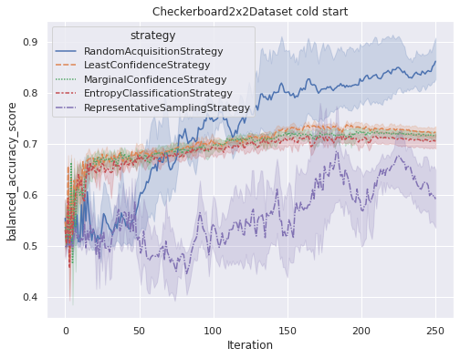
(a)

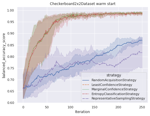
(b)

Figure 9: Performance curves over serial query iterations of selected active learning strategies on the Checkerboard2x2Dataset from Konyushkova et al. (2017). The left figure shows the balanced accuracy given a cold start task configuration, the right figure shows the performance given a warm start configuration.

Each of the datasets can be downloaded and processed into PyTorch Dataset objects through a simple API. Furthermore, we provide additional facilities to turn them into PyRelationAL DataManager objects that emulate cold and warm start AL initialisations with arbitrary train-validation-test splits and canonical splits (where applicable) for pain-free benchmarking.

In Figure 9, we show the performance curves over query iterations using a Gaussian process classifier with 5 different budgeted AL strategies on the Checkerboard2x2 dataset from Konyushkova et al. (2017). Our intent with this example is first to show drastic economies that can be obtained with active learning in early stages of labelling (i.e. AL is useful!) and secondly how dramatically these curves may change based on the task configuration within a dataset. We show the importance of the initial AL task configurations within datasets and demonstrate that there is no free-lunch amongst the AL strategies. Such results motivate the collection of datasets and task configurations, as well our modular approach to constructing methods so that researchers can modify and study the behaviours of novel strategies quickly. We provide a more comprehensive comparative analysis across the currently available datasets in Table 2 with details on the experimental setup as used here in Appendix Appendix E. Comparative analysis on selected strategies and datasets in PyRelationAL..

Appendix E. Comparative analysis on selected strategies and datasets in PyRelationAL.

In this section we perform a simple empirical comparative analysis of selected serial active learning strategies constructed with the informativeness measures in Table 1 across the current datasets in PyRelationAL. Serial active learning strategies perform one instance queries at each query loop iteration such that

$$Q_{k}=\operatorname*{argmax}_{q\in\mathcal{U}_{k}}I(q),$$

and the strategy is mainly driven by the choice of informativeness measure $I(\cdot)$. We remind that our aim here is to show the different components at play when creating AL experiments and assessing the resulting performances of strategies rather than advocating for any method.

Inspired by Konyushkova et al. (Konyushkova et al., 2017) and Yang and Loog (Yang and Loog, 2018), we assess our strategies on each dataset in two AL task configurations with respect to the ML task type.

• Cold-start classification: 1 observation for each class represented in the training set is labelled and the rest unlabeled.

• Warm-start classification: a randomly sampled 10 percent of the training set is labelled, the rest is unlabelled.

• Cold-start regression: the two observations with highest euclidean pairwise distance in the train set are labelled, the rest is unlabelled.

• Warm-start regression: a randomly sampled 10 percent of the training set is labelled, the rest is unlabelled.

Experimental setup

For each dataset, we use a 5-fold cross-validation setup (stratified for classification task). We generate a warm and cold start initialisation for each of these splits to set up an AL experiment. A single observation is queried at the end of each AL iteration, i.e. referred to the oracle for labelling. For small datasets (<300 observations in the training split) we run the query loop until all available observations in the training set are labelled. For larger datasets we set a maximum query budget of 250 iterations.

For the sake of simplicity, we used the same Gaussian process classifier (GPC) for each of the experiments on classification datasets and the same Gaussian process regressor (GPR) for the regression datasets. Both GPC and GPR utilise a RBF kernel. The model is trained anew at each AL query iteration. For both models, the prior is assumed to be constant and zero. The parameters of the kernel are optimized by maximizing the log marginal likelihood with the LBFGS algorithm. Details of the GPR implementation can be found in Algorithm 2.1 of Rasmussen and Williams (Rasmussen and Williams, 2006). The GPC implements the logistic link function based on Laplace approximation. Details of its implementation can be found in Algorithms 3.1, 3.2, and 5.1 of Rasmussen and Williams (Rasmussen and Williams, 2006).

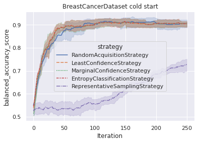
(a) Airfoil cold start

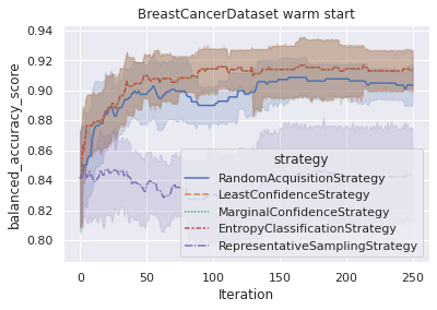
(b) Aifoil warm start

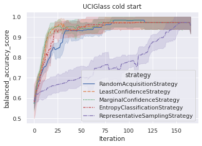
(c) Energy cold start

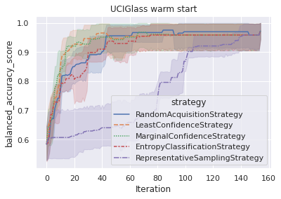
(d) Energy warm start

Figure 10: Plots of AL strategy performance on selected classification datasets,

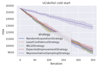
(a) Airfoil cold start

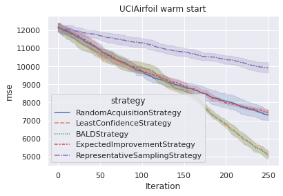
(b) Aifoil warm start

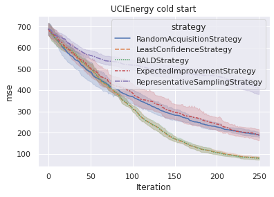
(c) Energy cold start

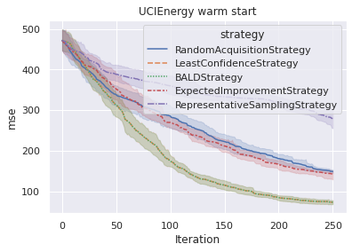
(d) Energy warm start

Figure 11: Plots of AL strategy performance on selected regression datasets.

At each query iteration, we record the model’s balanced accuracy score for classification datasets and mean square error (MSE) for regression datasets on the respective hold-out test sets. We aggregate the performance curves over the AL iterations showing the mean performance and 95% confidence intervals over the data splits as displayed in Figures 10 and 11. We also aggregate the area under each AL iteration performance curve (shortened to IPAUC), this is a single number where higher numbers denote better performance of the strategy in classification and lower numbers are better in regression. We report the mean IPAUC score and standard deviations over all the curves. Obviously, different metrics can be used for the "performance" in the IPAUC score.

Active learning strategies

To keep the performance curves from being too cluttered in this paper, we report the performance on a chosen few strategies. For classification tasks, we use the 1) random acquisition, 2) least confidence, 3) margin confidence, 4) entropy, and 5) representative sampling strategies. For regression tasks, we use the 1) random acquisition, 2) least confidence, 3) BALD, 4) expected improvement, and 5) representative sampling strategies. These represent a small sample of methods coming from different families of AL approaches based on uncertainty sampling and diversity sampling techniques (Settles, 2012; Monarch, 2021).

All experiments were run on a single workstation with an Intel(R) Xeon(R) E5-1650 v3 CPU clocked at 3.50GHz and 64GB memory.

Results and discussion

First and foremost, as can be seen in the AL performance curves of Figures 10 and 11, considerable performance gains can be made economically via AL. We can see comparable results for models with far less annotated observations than those using the full dataset. The gains are especially obvious in cold start settings as shown by the results obtained for the Glass dataset in Figure 10c. However, we can also see that certain strategies bring benefits later on such as the BALD strategy in warm start Airfoil dataset (Figure 11b). As Tables 3 through 6 show, in equally many cases AL does not bring any tangible benefits compared to the baseline of randomly acquiring labels for samples.

Assessment of the active learning strategies requires consideration of several factors acting in conjunction: the dataset, the model class used, the way under which uncertainty is measured from the model (if relevant for the informativeness measure), and obviously the strategy itself. Below we discuss some of these considerations with reference to the results across Tables 3 to 6 and Figures 10 and 11.

The dataset and associated ML task have an effect on the AL performance through the model as a task may be too simple to solve for a model — as is evident by the saturated and largely non-differentiable IPAUC scores in SynthClass1 and SynthClass2 for the GPC. The converse may also be true as demonstrated by the GPC’s inability to effectively improve its scores in the high dimensional StriatumMini dataset. In these cases, the choice of AL strategy does little to change performances. Properties of the dataset and model have strong effects on the query suggestions of the informativeness measures. Uncertainty sampling methods can often be myopic and focus heavily on samples near the decision boundary for discriminative models (Settles, 2012). This is helpful in datasets where representative instances have been labelled and the uncertainty sampling techniques may exploit the models uncertainty around classification boundaries to perform queries. On the other hand one can imagine how this may be detrimental in regression datasets with many outliers far away from majority of the dataset density that may be selected for annotation by uncertainty sampling techniques and waste query budget. This is why random acquisition is such a good baseline for pool based sampling scenarios as it naturally favours dense areas of the input space, whilst still having an element of exploration to overcome initial label bias (Monarch, 2021).

The choice of model affects strategies that utilise its notion of uncertainty to form informativeness measures. For example, the Gaussian process estimators we have utilised for the experiments provide principled measures of uncertainty. Meanwhile, a neural network can output class probabilities which can then be used to derive uncertainty estimates for informativeness measures. However, this is generally considered a poor uncertainty measure. Neural networks tend to produce pathologically overconfident predictions and struggle to quantify their uncertainty when applied on corrupted or previously unseen data (Ovadia et al., 2019; Hendrycks and Gimpel, 2016). Bayesian modelling (Ghahramani, 2015) as we have done with the GPs provides a theoretically rigorous approach to perform probabilistic inference also for deep neural networks. Seemingly these Bayesian neural networks (BNNs) combine the best of both worlds - the modelling complexity of a deep model augmented with uncertainty estimates through probabilistic inference over the weights of the neural network. Unfortunately the high computational cost of performing proper Bayesian inference restricts our use to using approximations. Many approximate Bayesian inference methods exist — such as MCDropout (Gal and Ghahramani, 2016) and SWAG (Maddox et al., 2019) — and each bring their own strengths, limitations, and hyperparameters that one can consider when assessing their downstream effects on AL strategies. Strategies designed to operate on committees and ensembles of models such as query-by-disagreement and query-by-committee algorithms work on similar principles and the collective of models gives rise informativeness measures whose quality and characteristics are dependent on its members.

As outlined in Appendix A, AL strategies can be defined through compositions of informativeness measures and query selection algorithms. Ultimately, the choice of strategy should be aligned with the objective of the practitioner. One objective of the active learning strategy can be to exploit model uncertainty to reduce classification error. This is useful for fine-tuning a model’s classification boundary and here uncertainty sampling techniques — such as the least confidence, margin, and entropy — succeed when ample representative data points are available as in the warm start configuration of Checkerboard2x2 in Figure 9b. Conversely, if the objective is to initially explore the input feature space, the serial uncertainty sampling strategies we have created can struggle immensely compared to random sampling baseline in Checkerboard2x2 cold start configuration in Figure 9a. This occurs as the myopic uncertainty sampling technique focuses its querying budget on refining the model’s classification boundary between the two initially labelled instances instead of exploring across its region of identically labelled areas diagonally across the plane. This can be overcome by adapting the query selection algorithm to balance the maximal informativeness coming from the informativeness function with another exploration utility measure. This interplay with informativeness measures, query selection, and their compositions — along with the considerations we have discussed above — give rise to the plethora of active learning strategies in literature and many yet unexplored avenues of research.

Table 3: IPAUC scores on balanced accuracy scores on a cold-start task configurations. Highest mean scores are bolded.

Classification cold start IPAUC (balanced accuracy)
	Random sampling	Least confidence	Margin	Entropy	Representativeness
UCIParkinsons	0.7202$\pm$0.0752	0.7471$\pm$0.0928	0.7422$\pm$0.1000	0.7343$\pm$0.1030	0.6876$\pm$0.0639
UCIGlass	0.9275$\pm$0.0250	0.9307$\pm$0.0277	0.9418$\pm$0.0203	0.9307$\pm$0.0278	0.7689$\pm$0.0372
UCISeeds	0.8885$\pm$0.0318	0.8842$\pm$0.0329	0.8839$\pm$0.0346	0.8797$\pm$0.0310	0.8522$\pm$0.0454
StriatumMini	0.4980$\pm$0.0000	0.4980$\pm$0.0000	0.4980$\pm$0.0000	0.4980$\pm$0.0000	0.4980$\pm$0.0000
GaussianClouds	0.5087$\pm$0.0068	0.5190$\pm$0.0150	0.5352$\pm$0.0325	0.5416$\pm$0.0250	0.4833$\pm$0.0152
Checkerboard2x2	0.7253$\pm$0.0366	0.6996$\pm$0.0066	0.6918$\pm$0.0087	0.6835$\pm$0.0109	0.5570$\pm$0.0409
Checkerboard4x4	0.5110$\pm$0.0086	0.5377$\pm$0.0138	0.5388$\pm$0.0103	0.5335$\pm$0.0076	0.4965$\pm$0.0120
BreastCancer	0.8741$\pm$0.0145	0.8774$\pm$0.0181	0.8765$\pm$0.0201	0.8782$\pm$0.0185	0.6011$\pm$0.0160
SynthClass1	0.9799$\pm$0.0148	0.9800$\pm$0.0149	0.9800$\pm$0.0151	0.9798$\pm$0.0150	0.9739$\pm$0.0122
SynthClass2	0.9718$\pm$0.0093	0.9918$\pm$0.0019	0.9924$\pm$0.0023	0.9922$\pm$0.0022	0.7295$\pm$0.2045

Table 4: IPAUC scores on balanced accuracy scores on a warm-start task configurations. Highest mean scores are bolded.

Classification warm start IPAUC (balanced accuracy)
	Random sampling	Least confidence	Margin	Entropy	Representativeness
UCIParkinsons	0.7645$\pm$0.0753	0.7520$\pm$0.0749	0.7510$\pm$0.0751	0.7363$\pm$0.0692	0.7341$\pm$0.1007
UCIGlass	0.9198$\pm$0.0470	0.9300$\pm$0.0487	0.9294$\pm$0.0476	0.9085$\pm$0.0430	0.7592$\pm$0.0581
UCISeeds	0.8804$\pm$0.0524	0.8832$\pm$0.0473	0.8801$\pm$0.0495	0.8839$\pm$0.0482	0.8830$\pm$0.0477
StriatumMini	0.4980$\pm$0.0000	0.4980$\pm$0.0000	0.4980$\pm$0.0000	0.4980$\pm$0.0000	0.4980$\pm$0.0000
GaussianClouds	0.6339$\pm$0.0067	0.6385$\pm$0.0097	0.6385$\pm$0.0097	0.6371$\pm$0.0111	0.6313$\pm$0.0053
Checkerboard2x2	0.7731$\pm$0.0228	0.9410$\pm$0.0249	0.9410$\pm$0.0249	0.9391$\pm$0.0285	0.7522$\pm$0.0607
Checkerboard4x4	0.5330$\pm$0.0153	0.5787$\pm$0.0214	0.5787$\pm$0.0215	0.5749$\pm$0.0195	0.5192$\pm$0.0149
BreastCancer	0.8942$\pm$0.0133	0.9043$\pm$0.0152	0.9043$\pm$0.0152	0.9043$\pm$0.0152	0.8353$\pm$0.0307
SynthClass1	0.9772$\pm$0.0058	0.9708$\pm$0.0082	0.9708$\pm$0.0082	0.9708$\pm$0.0082	0.9721$\pm$0.0105
SynthClass2	0.9959$\pm$0.0002	0.9960$\pm$0.0000	0.9960$\pm$0.0000	0.9960$\pm$0.0000	0.9957$\pm$0.0006

Table 5: IPAUC scores on mean square error on a cold-start task configurations. The lowest average mean square error is highlighted in bold.

Regression cold start IPAUC (MSE)
	Random sampling	Least confidence	BALD (Greedy)	Expected Improvement	Representativeness
SynthReg1	3.8077$\pm$1.0611	2.6635$\pm$0.5459	2.6635$\pm$0.5459	3.9732$\pm$1.6982	19.5705$\pm$8.7593
SynthReg2	13.3700$\pm$2.6140	0.0695$\pm$0.0636	0.0695$\pm$0.0636	0.9258$\pm$0.7598	500323.3267$\pm$95982.3408
UCIConcrete	1466.6133$\pm$71.6872	1472.8128$\pm$62.5106	1472.8371$\pm$62.4894	1474.8031$\pm$62.7577	1481.3249$\pm$63.4108
UCIEnergy	353.9005$\pm$30.3188	289.1917$\pm$15.2118	289.9866$\pm$16.1892	368.2726$\pm$40.6429	512.3891$\pm$25.3077
UCIPower	195496.1115$\pm$592.6507	198241.1702$\pm$733.1015	197934.2773$\pm$481.0792	195277.5576$\pm$874.4688	202216.1389$\pm$115.2624
WineQuality	26.3305$\pm$0.5950	29.4237$\pm$0.4255	29.6481$\pm$0.3058	26.2508$\pm$0.7875	30.1553$\pm$0.5857
UCIYacht	191.1043$\pm$106.0610	77.5529$\pm$5.6734	77.5529$\pm$5.6734	100.2691$\pm$32.6666	257.9830$\pm$81.8572
UCIAirfoil	11981.1223$\pm$248.5694	11891.0634$\pm$163.4600	11941.9477$\pm$120.2786	12129.1591$\pm$250.5744	14119.5660$\pm$290.1798
Diabetes	74877.8421$\pm$28927.1300	14171.5626$\pm$2047.0813	14171.5626$\pm$2047.0813	42432.5783$\pm$8133.3468	257918.0641$\pm$78686.9622

Table 6: IPAUC scores on mean square error on a warm-start task configurations. The lowest average mean square error is highlighted in bold.

Regression warm start IPAUC (MSE)
	Random sampling	Least confidence	BALD (Greedy)	Expected Improvement	Representativeness
SynthReg1	0.0922$\pm$0.1831	0.0138$\pm$0.0276	0.0138$\pm$0.0276	0.2684$\pm$0.5361	1.1291$\pm$2.2483
SynthReg2	15.1984$\pm$7.6929	1.3826$\pm$0.8757	1.3826$\pm$0.8757	2.8461$\pm$2.5169	142.2482$\pm$120.9354
UCIConcrete	1418.5645$\pm$88.1003	1424.9998$\pm$103.5379	1424.9998$\pm$103.5379	1429.0867$\pm$101.5682	1426.0738$\pm$104.0563
UCIEnergy	264.0951$\pm$21.3812	189.2541$\pm$16.0807	189.2541$\pm$16.0807	257.9486$\pm$18.4998	352.7991$\pm$19.1642
UCIPower	148798.2169$\pm$1249.1972	151130.8620$\pm$1005.3887	151087.9637$\pm$1039.0975	148664.4422$\pm$1016.8802	152460.5149$\pm$1267.7397
WineQuality	22.2955$\pm$0.6630	24.3891$\pm$0.5978	24.3565$\pm$0.5937	22.7723$\pm$0.6329	24.3539$\pm$0.5861
UCIYacht	84.8051$\pm$46.0703	38.1764$\pm$11.7308	38.1764$\pm$11.7308	154.5418$\pm$67.1644	178.9344$\pm$72.3744
UCIAirfoil	9407.7984$\pm$329.1265	8881.8400$\pm$265.1430	8882.0060$\pm$266.4904	9449.2188$\pm$160.0512	10990.5605$\pm$270.7223
Diabetes	78962.3416$\pm$10136.6245	17453.1527$\pm$3539.8087	17453.1527$\pm$3539.8087	51879.1983$\pm$12366.5705	234665.9027$\pm$52643.9754

Appendix F. Comparison with existing AL software packages

Table 7: Open source libraries for AL and features available. (*) ModAL can work with models defined in Keras and PyTorch via additional libraries such as Skorch Tietz et al. (2017) which provides them with an interface akin to Scikit-learn estimators. ($\dagger$) Scikit-activeml lists a planned update for regression strategies as does ALiPY. ($\ddagger$) Google’s AL playground has utilities for defining a dataset compatible with the sample strategies, as well as sample datasets to test this utility, but no verification on whether these datasets have been used for active learning in literature nor utilities for setting up AL task configurations.

Name (Year)	Main ML framework	Additional ML frameworks officially supported	Strategies Classification	Strategies Regression	Bayesian approximation	Explicit data managing	Datasets	Licence
Google Active Learning (2019)	Keras/TF	None	Yes	No	No	No	Yes$\ddagger$	Apache 2.0
JCLAL Reyes et al. (2016) (2016)	Weka/ MULAN	None	Yes	No	No	Yes	No	GPL 3.0
scikit-activeml Kottke et al. (2021) (2021)	Scikit-learn	None	Yes	No$\dagger$	No	No	No	BSD-3-Clause
AliPy Tang et al. (2019) (2019)	Generic	NA	Yes	No$\dagger$	No	Yes	No	BSD-3-Clause
LibAcT Yang et al. (2017) (2017)	Scikit-learn	None	Yes	No	No	Yes	No	BSD-2-Clause
CardinAL Abraham and Dreyfus-Schmidt (2022) (2022)	Scikit-learn	None	Yes	No	No	No	No	Apache 2.0
BAAL Atighehchian et al. (2020) (2020)	PyTorch	Scikit-learn	Yes	Yes	Yes	Yes	No	Apache 2.0
ModAL Danka and Horvath (2018) (2018)	Scikit-learn	Keras/PyTorch*	Yes	Yes	No	Yes	No	MIT
PyRelationAL (2022)	Generic/ PyTorch	Scikit-learn/TF/ Keras/Jax	Yes	Yes	Yes	Yes	Yes	Apache 2.0

PyRelationAL was developed under careful consideration of features available within the existing AL ecosystem, coupled with our vision to create a researcher-first library for AL research and development. To accommodate the growing complexity, advancements in new ML infrastructures and encourage user construction of complex AL pipelines and strategies, we strove to make implementation of data managers, ML models, AL strategies, and oracle interfaces as flexible and productive as possible. This is achieved through a modular framework which we described in Section 2.

There are a number of open source libraries dedicated to AL whose features are summarised in Table 7. As the table shows, most libraries are tied to a particular ML framework with specific strategies revolving around the available ML model types, all with differing levels of coverage both across classification and regression tasks. Each library comes with different goals in mind and should be appreciated for addressing different needs in open source research. For example, ModAL by Danka and Horvath (2018) is an excellent modular python library for AL built with Scikit-learn as a basis for models. Its design emphasis on modularity and extensibility of the model construction and strategies makes it the most similar to our work.

Yet we differ to this and other libraries by making the user explicitly concern themselves with the construction and behaviour of an active learning Pipeline instance as the composition of a DataManager, ModelManager, AL Strategy, and Oracle. The flexible nature of our modules may be seen as a limitation that incurs additional development overhead compared to other libraries but we believe this trade-off is practical and useful to researchers exploring new behaviours within each of these components. In particular, using a ModelManager enables PyRelationAL to be agnostic to the user’s choice of ML model implementation and framework, which lets it stay relevant in face of an ever-changing ML landscape. Similarly, an extensible Strategy class encourages user development of new active learning strategies. Another considerable differentiation to other AL libraries is the Oracle interface which enables interaction with various annotation tools should the active learning pipeline be deployed.

Finally, as we outline in Section Appendix D. Benchmark datasets and AL tasks., another important contribution of our library is an API for downloading selected datasets and constructing AL benchmarks or tasks based on existing AL literature. This new offering should help researchers quickly benchmark their proposed strategies across a range of established or challenging benchmarks and help identify regimes under which a given strategy shows success or difficulties. As such we believe that PyRelationAL offers a compelling and complete set of features that is complementary and additive to the existing ML and the AL tools ecosystem. In the next section we describe how our modules enable quick development of AL with the practical flexibility to create novel pipelines and strategies.

References

- Abdelwahab and Busso (2019) Mohammed Abdelwahab and Carlos Busso. Active learning for speech emotion recognition using deep neural network. In 2019 8th International Conference on Affective Computing and Intelligent Interaction (ACII), pages 1–7. IEEE, 2019.
- Abraham and Dreyfus-Schmidt (2022) Alexandre Abraham and Léo Dreyfus-Schmidt. Cardinal, a metric-based active learning framework. Software Impacts, 12:100250, 2022. ISSN 2665-9638. doi: https://doi.org/10.1016/j.simpa.2022.100250. URL https://www.sciencedirect.com/science/article/pii/S2665963822000173.
- Atighehchian et al. (2020) Parmida Atighehchian, Frédéric Branchaud-Charron, and Alexandre Lacoste. Bayesian active learning for production, a systematic study and a reusable library. CoRR, abs/2006.09916, 2020. URL https://arxiv.org/abs/2006.09916.
- Bertin et al. (2022) Paul Bertin, Jarrid Rector-Brooks, Deepak Sharma, Thomas Gaudelet, Andrew Anighoro, Torsten Gross, Francisco Martinez-Pena, Eileen L Tang, Cristian Regep, Jeremy Hayter, et al. Recover: sequential model optimization platform for combination drug repurposing identifies novel synergistic compounds in vitro. arXiv preprint arXiv:2202.04202, 2022.
- Bradbury et al. (2018) James Bradbury, Roy Frostig, Peter Hawkins, Matthew James Johnson, Chris Leary, Dougal Maclaurin, George Necula, Adam Paszke, Jake VanderPlas, Skye Wanderman-Milne, and Qiao Zhang. JAX: composable transformations of Python+NumPy programs, 2018. URL http://github.com/google/jax.
- Brinker (2003) Klaus Brinker. Incorporating diversity in active learning with support vector machines. In Proceedings of the Twentieth International Conference on International Conference on Machine Learning, ICML’03, page 59–66. AAAI Press, 2003. ISBN 1577351894.
- Brochu et al. (2010) Eric Brochu, Vlad M Cora, and Nando De Freitas. A tutorial on bayesian optimization of expensive cost functions, with application to active user modeling and hierarchical reinforcement learning. arXiv preprint arXiv:1012.2599, 2010.
- Cai et al. (2013) Wenbin Cai, Ya Zhang, and Jun Zhou. Maximizing expected model change for active learning in regression. In 2013 IEEE 13th International Conference on Data Mining, pages 51–60, 2013. doi: 10.1109/ICDM.2013.104.
- Chollet et al. (2015) François Chollet et al. Keras. https://keras.io, 2015.
- Cohn et al. (1994) David Cohn, Les Atlas, and Richard Ladner. Improving generalization with active learning. Machine Learning, 15(2):201–221, May 1994. ISSN 1573-0565. doi: 10.1007/BF00993277. URL https://doi.org/10.1007/BF00993277.
- Cortez et al. (2009) Paulo Cortez, António Cerdeira, Fernando Almeida, Telmo Matos, and José Reis. Modeling wine preferences by data mining from physicochemical properties. Decision Support Systems, 47(4):547–553, 2009. ISSN 0167-9236. doi: https://doi.org/10.1016/j.dss.2009.05.016. URL https://www.sciencedirect.com/science/article/pii/S0167923609001377. Smart Business Networks: Concepts and Empirical Evidence.
- Dagan and Engelson (1995) Ido Dagan and Sean P. Engelson. Committee-based sampling for training probabilistic classifiers. In Proceedings of the Twelfth International Conference on International Conference on Machine Learning, ICML’95, page 150–157, San Francisco, CA, USA, 1995. Morgan Kaufmann Publishers Inc. ISBN 1558603778.
- Danka and Horvath (2018) Tivadar Danka and Peter Horvath. modal: A modular active learning framework for python. arXiv preprint arXiv:1805.00979, 2018.
- Dasgupta and Hsu (2008) Sanjoy Dasgupta and Daniel Hsu. Hierarchical sampling for active learning. In Proceedings of the 25th International Conference on Machine Learning, ICML ’08, page 208–215, New York, NY, USA, 2008. Association for Computing Machinery. ISBN 9781605582054. doi: 10.1145/1390156.1390183. URL https://doi.org/10.1145/1390156.1390183.
- De Ath et al. (2021) George De Ath, Richard M Everson, Alma AM Rahat, and Jonathan E Fieldsend. Greed is good: Exploration and exploitation trade-offs in bayesian optimisation. ACM Transactions on Evolutionary Learning and Optimization, 1(1):1–22, 2021.
- Deng et al. (2009) J. Deng, W. Dong, R. Socher, L.-J. Li, K. Li, and L. Fei-Fei. ImageNet: A Large-Scale Hierarchical Image Database. In Computer Vision and Pattern Recognition, 2009.
- Der Kiureghian and Ditlevsen (2009) Armen Der Kiureghian and Ove Ditlevsen. Aleatory or epistemic? does it matter? Structural Safety, 31(2):105–112, 2009.
- Du et al. (2017) Bo Du, Zengmao Wang, Lefei Zhang, Liangpei Zhang, Wei Liu, Jialie Shen, and Dacheng Tao. Exploring representativeness and informativeness for active learning. IEEE Transactions on Cybernetics, 47(1):14–26, 2017. doi: 10.1109/TCYB.2015.2496974.
- Dua and Graff (2017) Dheeru Dua and Casey Graff. UCI machine learning repository, 2017.
- Efron et al. (2004) Bradley Efron, Trevor Hastie, Iain Johnstone, and Robert Tibshirani. Least angle regression. The Annals of Statistics, 32(2):407 – 499, 2004. doi: 10.1214/009053604000000067. URL https://doi.org/10.1214/009053604000000067.
- Gal and Ghahramani (2016) Yarin Gal and Zoubin Ghahramani. Dropout as a bayesian approximation: Representing model uncertainty in deep learning. In International Conference on Machine Learning, pages 1050–1059. PMLR, 2016.
- Gardner et al. (2018) Jacob R Gardner, Geoff Pleiss, David Bindel, Kilian Q Weinberger, and Andrew Gordon Wilson. Gpytorch: Blackbox matrix-matrix gaussian process inference with gpu acceleration. In Advances in Neural Information Processing Systems, 2018.
- Ghahramani (2015) Zoubin Ghahramani. Probabilistic machine learning and artificial intelligence. Nature, 521(7553):452–459, 2015.
- Guo and Schuurmans (2007) Yuhong Guo and Dale Schuurmans. Discriminative batch mode active learning. In Proceedings of the 20th International Conference on Neural Information Processing Systems, NIPS’07, page 593–600, Red Hook, NY, USA, 2007. Curran Associates Inc. ISBN 9781605603520.
- Heek et al. (2020) Jonathan Heek, Anselm Levskaya, Avital Oliver, Marvin Ritter, Bertrand Rondepierre, Andreas Steiner, and Marc van Zee. Flax: A neural network library and ecosystem for JAX, 2020. URL http://github.com/google/flax.
- Hendrycks and Gimpel (2016) Dan Hendrycks and Kevin Gimpel. A baseline for detecting misclassified and out-of-distribution examples in neural networks. arXiv preprint arXiv:1610.02136, 2016.
- Hie et al. (2020) Brian Hie, Bryan D Bryson, and Bonnie Berger. Leveraging uncertainty in machine learning accelerates biological discovery and design. Cell Systems, 11(5):461–477, 2020.
- Hoi et al. (2006) Steven CH Hoi, Rong Jin, Jianke Zhu, and Michael R Lyu. Batch mode active learning and its application to medical image classification. In Proceedings of the 23rd International Conference on Machine Learning, pages 417–424, 2006.
- Houlsby et al. (2011a) Neil Houlsby, Ferenc Huszár, Zoubin Ghahramani, and Máté Lengyel. Bayesian active learning for classification and preference learning. arXiv preprint arXiv:1112.5745, 2011a.
- Houlsby et al. (2011b) Neil Houlsby, Ferenc Huszár, Zoubin Ghahramani, and Máté Lengyel. Bayesian active learning for classification and preference learning. arXiv preprint arXiv:1112.5745, 2011b.
- Hu et al. (2020) Weihua Hu, Matthias Fey, Marinka Zitnik, Yuxiao Dong, Hongyu Ren, Bowen Liu, Michele Catasta, and Jure Leskovec. Open graph benchmark: Datasets for machine learning on graphs. Advances in Neural Information Processing Systems, 33:22118–22133, 2020.
- Huang et al. (2021) Kexin Huang, Tianfan Fu, Wenhao Gao, Yue Zhao, Yusuf Roohani, Jure Leskovec, Connor W Coley, Cao Xiao, Jimeng Sun, and Marinka Zitnik. Therapeutics data commons: Machine learning datasets and tasks for drug discovery and development. arXiv preprint arXiv:2102.09548, 2021.
- Huang et al. (2015) Sheng-Jun Huang, Songcan Chen, and Zhi-Hua Zhou. Multi-label active learning: Query type matters. In Proceedings of the 24th International Conference on Artificial Intelligence, IJCAI’15, page 946–952. AAAI Press, 2015. ISBN 9781577357384.
- Kirsch et al. (2019) Andreas Kirsch, Joost Van Amersfoort, and Yarin Gal. Batchbald: Efficient and diverse batch acquisition for deep bayesian active learning. Advances in Neural Information Processing Systems, 32, 2019.
- Konyushkova et al. (2015) Ksenia Konyushkova, Raphael Sznitman, and Pascal V. Fua. Introducing geometry in active learning for image segmentation. 2015 IEEE International Conference on Computer Vision (ICCV), pages 2974–2982, 2015.
- Konyushkova et al. (2017) Ksenia Konyushkova, Raphael Sznitman, and Pascal Fua. Learning active learning from data. Advances in Neural Information Processing Systems, 30, 2017.
- Kottke et al. (2021) Daniel Kottke, Marek Herde, Tuan Pham Minh, Alexander Benz, Pascal Mergard, Atal Roghman, Christoph Sandrock, and Bernhard Sick. scikitactiveml: A library and toolbox for active learning algorithms. Preprints, 2021. doi: 10.20944/preprints202103.0194.v1. URL https://github.com/scikit-activeml/scikit-activeml.
- Lakshminarayanan et al. (2017) Balaji Lakshminarayanan, Alexander Pritzel, and Charles Blundell. Simple and Scalable Predictive Uncertainty Estimation using Deep Ensembles. arXiv:1612.01474 [cs, stat], November 2017. URL http://arxiv.org/abs/1612.01474. arXiv: 1612.01474.
- Lewis and Catlett (1994) David D. Lewis and Jason Catlett. Heterogeneous uncertainty sampling for supervised learning. In William W. Cohen and Haym Hirsh, editors, Machine Learning Proceedings 1994, pages 148–156. Morgan Kaufmann, San Francisco (CA), 1994. ISBN 978-1-55860-335-6. doi: https://doi.org/10.1016/B978-1-55860-335-6.50026-X. URL https://www.sciencedirect.com/science/article/pii/B978155860335650026X.
- Little et al. (2007) Max A. Little, Patrick E. McSharry, Stephen J. Roberts, Declan AE Costello, and Irene M. Moroz. Exploiting nonlinear recurrence and fractal scaling properties for voice disorder detection. BioMedical Engineering OnLine, 6(1):23, Jun 2007.
- Lucchi et al. (2012) Aurélien Lucchi, Yunpeng Li, Kevin Smith, and Pascal Fua. Structured image segmentation using kernelized features. In European conference on computer vision, pages 400–413. Springer, 2012.
- Lucchi et al. (2013) Aurélien Lucchi, Yunpeng Li, and Pascal Fua. Learning for structured prediction using approximate subgradient descent with working sets. In 2013 IEEE Conference on Computer Vision and Pattern Recognition, pages 1987–1994, 2013. doi: 10.1109/CVPR.2013.259.
- Maddox et al. (2019) Wesley J. Maddox, Timur Garipov, Pavel Izmailov, Dmitry Vetrov, and Andrew Gordon Wilson. A Simple Baseline for Bayesian Uncertainty in Deep Learning. Curran Associates Inc., Red Hook, NY, USA, 2019.
- Mehrjou et al. (2021) Arash Mehrjou, Ashkan Soleymani, Andrew Jesson, Pascal Notin, Yarin Gal, Stefan Bauer, and Patrick Schwab. GeneDisco: A Benchmark for Experimental Design in Drug Discovery. arXiv:2110.11875 [cs, stat], October 2021. arXiv: 2110.11875.
- Monarch (2021) Robert (Munro) Monarch. Human-In-the-Loop Machine Learning: Active Learning and Annotation for Human-Centered AI. Manning Publications Co. LLC, 2021. ISBN 978-1-61729-674-1.
- Nguyen and Smeulders (2004) Hieu T. Nguyen and Arnold Smeulders. Active learning using pre-clustering. In Proceedings of the Twenty-First International Conference on Machine Learning, ICML ’04, page 79, New York, NY, USA, 2004. Association for Computing Machinery. ISBN 1581138385. doi: 10.1145/1015330.1015349. URL https://doi.org/10.1145/1015330.1015349.
- Ovadia et al. (2019) Yaniv Ovadia, Emily Fertig, Jie Ren, Zachary Nado, David Sculley, Sebastian Nowozin, Joshua Dillon, Balaji Lakshminarayanan, and Jasper Snoek. Can you trust your model’s uncertainty? evaluating predictive uncertainty under dataset shift. Advances in Neural Information Processing Systems, 32, 2019.
- Paszke et al. (2019) Adam Paszke, Sam Gross, Francisco Massa, et al. Pytorch: An imperative style, high-performance deep learning library. In H. Wallach, H. Larochelle, A. Beygelzimer, F. d'Alché-Buc, E. Fox, and R. Garnett, editors, Advances in Neural Information Processing Systems 32, pages 8024–8035. Curran Associates, Inc., 2019. URL http://papers.neurips.cc/paper/9015-pytorch-an-imperative-style-high-performance-deep-learning-library.pdf.
- Pedregosa et al. (2011) F. Pedregosa, G. Varoquaux, A. Gramfort, V. Michel, B. Thirion, O. Grisel, M. Blondel, P. Prettenhofer, R. Weiss, V. Dubourg, J. Vanderplas, A. Passos, D. Cournapeau, M. Brucher, M. Perrot, and E. Duchesnay. Scikit-learn: Machine learning in Python. Journal of Machine Learning Research, 12:2825–2830, 2011.
- Phan et al. (2019) Du Phan, Neeraj Pradhan, and Martin Jankowiak. Composable effects for flexible and accelerated probabilistic programming in numpyro. arXiv preprint arXiv:1912.11554, 2019.
- Pinsler et al. (2019) Robert Pinsler, Jonathan Gordon, Eric Nalisnick, and José Miguel Hernández-Lobato. Bayesian batch active learning as sparse subset approximation. Advances in Neural Information Processing Systems, 32, 2019.
- Pozzolo et al. (2015) Andrea Dal Pozzolo, Olivier Caelen, Reid A. Johnson, and Gianluca Bontempi. Calibrating probability with undersampling for unbalanced classification. In 2015 IEEE Symposium Series on Computational Intelligence, pages 159–166, 2015. doi: 10.1109/SSCI.2015.33.
- Rasmussen and Williams (2006) Carl Edward Rasmussen and Christopher K. I. Williams. Gaussian processes for machine learning, volume 2. MIT Press, 2006.
- Ren et al. (2021) Pengzhen Ren, Yun Xiao, Xiaojun Chang, Po-Yao Huang, Zhihui Li, Brij B Gupta, Xiaojiang Chen, and Xin Wang. A survey of deep active learning. ACM Computing Surveys (CSUR), 54(9):1–40, 2021.
- Reyes et al. (2016) Oscar Reyes, Eduardo Pérez, María del Carmen Rodríguez-Hernández, Habib M. Fardoun, and Sebastián Ventura. Jclal: A java framework for active learning. Journal of Machine Learning Research, 17(95):1–5, 2016. URL http://jmlr.org/papers/v17/15-347.html.
- Russo et al. (2018) Daniel J Russo, Benjamin Van Roy, Abbas Kazerouni, Ian Osband, Zheng Wen, et al. A tutorial on thompson sampling. Foundations and Trends in Machine Learning, 11(1):1–96, 2018.
- Scheffer et al. (2001) Tobias Scheffer, Christian Decomain, and Stefan Wrobel. Active hidden markov models for information extraction. In Proceedings of the 4th International Conference on Advances in Intelligent Data Analysis, IDA ’01, page 309–318, Berlin, Heidelberg, 2001. Springer-Verlag. ISBN 3540425810.
- Settles (2012) Burr Settles. Uncertainty sampling. In Active Learning, Synthesis Lectures on Artificial Intelligence and Machine Learning, pages 11–21. Morgan & Claypool Publishers, 2012.
- Seung et al. (1992) H. S. Seung, M. Opper, and H. Sompolinsky. Query by committee. In Proceedings of the Fifth Annual Workshop on Computational Learning Theory, COLT ’92, page 287–294, New York, NY, USA, 1992. Association for Computing Machinery. ISBN 089791497X. doi: 10.1145/130385.130417. URL https://doi.org/10.1145/130385.130417.
- Shannon (1948) Claude Elwood Shannon. A mathematical theory of communication. The Bell System Technical Journal, 27:379–423, 1948. URL http://plan9.bell-labs.com/cm/ms/what/shannonday/shannon1948.pdf.
- Smith et al. (2018) Justin S Smith, Ben Nebgen, Nicholas Lubbers, Olexandr Isayev, and Adrian E Roitberg. Less is more: Sampling chemical space with active learning. The Journal of Chemical Physics, 148(24):241733, 2018.
- Sutton and Barto (2018) Richard S Sutton and Andrew G Barto. Reinforcement learning: An introduction. MIT press, 2018.
- Tang et al. (2019) Ying-Peng Tang, Guo-Xiang Li, and Sheng-Jun Huang. ALiPy: Active learning in python. Technical report, Nanjing University of Aeronautics and Astronautics, January 2019. URL https://github.com/NUAA-AL/ALiPy. available as arXiv preprint https://arxiv.org/abs/1901.03802.
- Tietz et al. (2017) Marian Tietz, Thomas J. Fan, Daniel Nouri, Benjamin Bossan, and skorch Developers. skorch: A scikit-learn compatible neural network library that wraps PyTorch, July 2017. URL https://skorch.readthedocs.io/en/stable/.
- Tkachenko et al. (2020-2022) Maxim Tkachenko, Mikhail Malyuk, Andrey Holmanyuk, and Nikolai Liubimov. Label Studio: Data labeling software, 2020-2022. URL https://github.com/heartexlabs/label-studio. Open source software available from https://github.com/heartexlabs/label-studio.
- Tran et al. (2017) Dustin Tran, Matthew D. Hoffman, Rif A. Saurous, Eugene Brevdo, Kevin Murphy, and David M. Blei. Deep probabilistic programming. In International Conference on Learning Representations, 2017.
- Tsanas and Xifara (2012) Athanasios Tsanas and Angeliki Xifara. Accurate quantitative estimation of energy performance of residential buildings using statistical machine learning tools. Energy and Buildings, 49:560–567, 2012. ISSN 0378-7788. doi: https://doi.org/10.1016/j.enbuild.2012.03.003. URL https://www.sciencedirect.com/science/article/pii/S037877881200151X.
- Tüfekci (2014) Pınar Tüfekci. Prediction of full load electrical power output of a base load operated combined cycle power plant using machine learning methods. International Journal of Electrical Power & Energy Systems, 60:126–140, 2014. ISSN 0142-0615. doi: https://doi.org/10.1016/j.ijepes.2014.02.027. URL https://www.sciencedirect.com/science/article/pii/S0142061514000908.
- Wang et al. (2019) Alex Wang, Yada Pruksachatkun, Nikita Nangia, Amanpreet Singh, Julian Michael, Felix Hill, Omer Levy, and Samuel Bowman. Superglue: A stickier benchmark for general-purpose language understanding systems. Advances in Neural Information Processing Systems, 32, 2019.
- Wu (2019) Dongrui Wu. Pool-based sequential active learning for regression. IEEE Transactions on Neural Networks and Learning Systems, 30(5):1348–1359, 2019. doi: 10.1109/TNNLS.2018.2868649.
- Xiong et al. (2014) Sicheng Xiong, Javad Azimi, and Xiaoli Z. Fern. Active learning of constraints for semi-supervised clustering. IEEE Transactions on Knowledge and Data Engineering, 26(1):43–54, 2014. doi: 10.1109/TKDE.2013.22.
- Yang et al. (2017) Yao-Yuan Yang, Shao-Chuan Lee, Yu-An Chung, Tung-En Wu, Si-An Chen, and Hsuan-Tien Lin. libact: Pool-based active learning in python. Technical report, National Taiwan University, October 2017. URL https://github.com/ntucllab/libact. available as arXiv preprint https://arxiv.org/abs/1710.00379.
- Yang and Loog (2018) Yazhou Yang and Marco Loog. A benchmark and comparison of active learning for logistic regression. Pattern Recognition, 83:401–415, 2018.
- Yeh (1998) I.-C. Yeh. Modeling of strength of high-performance concrete using artificial neural networks. Cement and Concrete Research, 28(12):1797–1808, 1998. ISSN 0008-8846. doi: https://doi.org/10.1016/S0008-8846(98)00165-3. URL https://www.sciencedirect.com/science/article/pii/S0008884698001653.
- Zhan et al. (2021) Xueying Zhan, Huan Liu, Qing Li, and Antoni B. Chan. A comparative survey: Benchmarking for pool-based active learning. In Zhi-Hua Zhou, editor, Proceedings of the Thirtieth International Joint Conference on Artificial Intelligence, IJCAI-21, pages 4679–4686. International Joint Conferences on Artificial Intelligence Organization, 8 2021. doi: 10.24963/ijcai.2021/634. URL https://doi.org/10.24963/ijcai.2021/634. Survey Track.