The Ages of Optically Bright Sub-Clusters in the Serpens Star-Forming Region

Abstract

The Serpens Molecular Cloud is one of the most active star-forming regions within 500 pc, with over one thousand of YSOs at different evolutionary stages. The ages of the member stars inform us about the star formation history of the cloud. In this paper, we develop a spectral energy distribution (SED) fitting method for nearby evolved (diskless) young stars from members of the Pleiades to estimate their ages, with a temperature scale adopted from APOGEE spectra. When compared with literature temperatures of selected YSOs in Orion, the SED fits to cool ($<5000$ K) stars have temperatures that differ by an average of $<\sim$ 50 K and have a scatter of $\sim 210$ K for both disk-hosting and diskless stars. We then apply this method to YSOs in the Serpens Molecular Cloud to estimate ages of optical members previously identified from Gaia DR2 astrometry data. The optical members in Serpens are concentrated in different subgroups with ages from $\sim 4$ Myr to $\sim 22$ Myr; the youngest clusters, W40 and Serpens South, are dusty regions that lack enough optical members to be included in this analysis. These ages establish that the Serpens Molecular Cloud has been forming stars for much longer than has been inferred from infrared surveys.

1 Introduction

The story of the star-forming history of a molecular cloud is told through its dust, gas, and member stars. The youngest members, the protostars, are still forming and are typically clustered in the densest regions of the cloud. Stars formed in previous bursts are often still located in small subclusters, while some have been dispersed throughout the cloud or were born in small groups. In many clouds the older stars are not co-located with the youngest stars, indicating that the site for star formation changes with time within a cloud complex (e.g., Getman et al., 2014b, a; Vázquez-Semadeni et al., 2018; Kounkel et al., 2018; Kristensen & Dunham, 2018; Liu et al., 2021).

The Serpens Molecular Cloud is one of the nearest clouds with vigorous ongoing star formation, second to only Orion among active star-forming sites within 500 pc. Historically the Serpens Main cluster (see review by Eiroa et al., 2008) and W40 (Kuhn et al. 2010; see also review by Rodney & Reipurth 2008) were recognized as primary sites of star formation in the complex; mid- and far-IR and X-ray surveys revealed vigorous ongoing star formation in the deeply embedded Serpens South cluster (Gutermuth et al., 2008; Povich et al., 2013; Mallick et al., 2013; Könyves et al., 2015; Dunham et al., 2015). Beyond these sub-clusters, recently-formed stars are sparse and hard to find (see review by Prato et al., 2008). Accurate astrometry and optical photometry from Gaia DR2 revealed the optical members, including some in new subclusters and some distributed throughout the cloud (Herczeg et al., 2019), while most candidate members that were outside the main star-forming sites have been identified as contaminants (see also Lee et al., 2021). The optical members that are distributed across the cloud likely formed in past epochs of star formation.

Table 1: Photometry selection criteria

	Pass-band	Criteria	Note
Gaia	$BP,RP$	parallax_over_error>10 astrometric_excess_noise<2 visibility_periods_used>8 phot_g_mean_flux_over_error>50
2MASS	$J,H,K$	ph_qual="AAA"
WISE	$W1,W2$	SNR>10 $\chi^{2}$<3	W1 and W2 are selected and treated independently.
Pan-STARRS	$g,r,i,z,y$	nDetections>5 gQfPerfect>0.85 rQfPerfect>0.85 iQfPerfect>0.85 zQfPerfect>0.85 imeanpsfmag - imeankronmag < 0.05 OR rmeanpsfmag - rmeankronmag < 0.05	Pan-STARRS data of a star will be used only if the data satisfy all the criteria.
APASS	$B,V,g^{\prime},r^{\prime},i^{\prime}$	-	$r/i_{\rm APASS}$ and $r/i_{\rm PS1}$ are treated as the same in SED fitting . If a star has both $r_{\rm PS1}$ (or $i_{\rm PS1}$) and $r_{\rm APASS}$ (or $i_{\rm APASS}$) data, then Pan-STARRS $r$ (or $i$) will be used.

Note. — A star will be included only if it passes both Gaia and 2MASS criteria, because the SED fitting method needs at least 4 pass-bands (Section 3.3) and Gaia and 2MASS pass-bands cover the full temperature range of Pleiades stars (Section 2.1, Figure 2 and Table 9). If a star passes both Gaia and 2MASS criteria and fails in WISE/Pan-STARRS/APASS criteria, it will be included and its WISE/Pan-STARRS/APASS photometry will not be used.

A comprehensive description of the star formation history of the Serpens Molecular Cloud requires estimates of when these member stars formed. However, accurate ages depend on estimates for the stellar properties, which are complicated by the variation of extinction across the cluster. Cluster ages can be estimated from HR diagrams (e.g. Erickson et al., 2015), the lithium depletion boundary (e.g. Basri et al., 1996; Binks & Jeffries, 2014), and the X-ray luminosity function (e.g. Getman et al., 2014b), with varying degrees of accuracy and systematic precision (see review by Soderblom et al., 2014). However, for the most common method, use of HR diagrams, few young stellar objects in the Serpens Molecular Cloud have measured temperatures and luminosities that could be used to estimate their age (e.g. Oliveira et al., 2013; Erickson et al., 2015). In the absence of spectroscopic measurements, photospheric properties are usually estimated by fitting SEDs with synthetic spectra (e.g., Bayo et al., 2008; Robitaille, 2017; Davies, 2020). This approach may introduce biases at cool temperaturesm where synthetic SEDs differ from observed SEDs (e.g. Bell et al. 2012 and Lançon et al. 2020; see also analysis of main-sequence M-dwarfs in Mann et al. 2015). Because nearby star-forming regions are mainly composed of low-mass stars (e.g., Luhman & Esplin, 2020), low-mass stars dominate isochronal age measurements for most nearby star-forming regions (e.g., Mayne et al., 2007; Bell et al., 2012; Zari et al., 2019); any systematic errors in their stellar properties propagate into (often unassessed) uncertainties in ages of star-forming regions.

In this paper, we develop a new SED fitting routine designed for young stars and then apply the fitting routine to optical members of Serpens to estimate stellar ages by comparing best-fit temperature and luminosities to model isochrones. In Section 2, we present the data, including data for the fitting method and for Serpens. In Section 3, details of the SED fitting method are described. In Section 4, we use the method on Serpens stars and derive their ages. In Section 5, we discuss the results, and the conclusions are summarized in Section 6.

2 Photometric data and cluster member selection

The results from this paper are obtained by fitting the SEDs of YSOs in Serpens using a grid of empirically measured SEDs of young stars. The grid is built with known members of the Pleiades and nearby young moving groups, following similar approaches by Bell et al. (2012) and Pecaut & Mamajek (2013). The Pleiades members are young ($\sim$110 Myr, Gaia Collaboration et al., 2018), nearby ($\sim$136 pc, Gaia Collaboration et al., 2018), have solar metallicity ($[Fe/H]\sim 0.03$, Soderblom et al., 2009), and for the cooler stars are magnetically active (see the effect of surface gravity in Section 3.8). The line-of-sight extinction to the Pleiades is negligible ($A_{V}=0.12$, Stauffer et al., 1998), so the photometry does not require any significant correction. This grid and our fitting methods are then tested using known members of Orion. The photometry used in this paper is obtained from 2MASS (Cutri et al., 2003; Skrutskie et al., 2019), ALLWISE (Cutri et al., 2021; Wright et al., 2019), Pan-STARRS1 (PS1, Chambers et al., 2016), APASS (the Apache Point Observatory Galactic Evolution Experiment, Henden et al., 2015), and Gaia EDR3 (Gaia Collaboration et al., 2021), with quality criteria described in Table 1.

The Pan-STARRS1 and APASS (SDSS-based) filters $r$, $i$ have slightly different transmission curves. Tonry et al. (2012) presents $g_{\rm SDSS}-g_{\rm PS1}$, $r_{\rm SDSS}-r_{\rm PS1}$, and $i_{\rm SDSS}-i_{\rm PS1}$ at $>\sim 4000$ K (their Figure 6, 7), showing that the difference in $g$ band is significant, while $r$ and $i$ bands have negligible difference. At $<\sim 4000$ K, stars in Kado-Fong et al. (2016) $r_{\rm APASS}$ is fainter than $r_{\rm PS1}$ by $\sim 0.07$ mag and $i_{\rm APASS}$ is fainter than $i_{\rm PS1}$ by $\sim 0.05$ mag. In addition, the APASS faint completeness limit (V=16) corresponds to $\sim 3700$ K for Pleiades, so this difference is not relevant for most stars. For example, among the selected Pleiades stars under 4000 K (178 stars), only 16 stars have APASS data, and all the 16 stars have Pan-STARRS data. Among the Orion stars used to test the SED fitting method, only 1 star under 4000 K has APASS data, indicating that the magnitude difference has a minor effect on the fitting method. In SED fitting, we use $g_{\rm APASS}$ and $g_{\rm PS1}$ separately, and treat $r$ and $i$ as the same. If a star has both $r_{\rm PS1}$ (or $i_{\rm PS1}$) and $r_{\rm APASS}$ (or $i_{\rm APASS}$) data, then Pan-STARRS $r$ (or $i$) will be used.

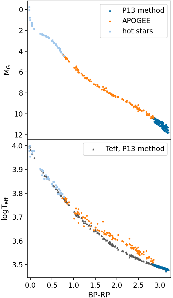
Figure 1: Color-magnitude diagram (top) and color-temperature relation (bottom) of the Pleiades stars in our sample, for cool stars with temperatures derived from Pecaut & Mamajek (2013) SED fits (deep blue dots), stars with APOGEE temperatures (orange dots), hotter stars with temperatures from other catalogs (light blue square), and (in the bottom panel) stars with APOGEE temperatures that also have temperatures assessed by Pecaut & Mamajek (2013) (gray triangle).

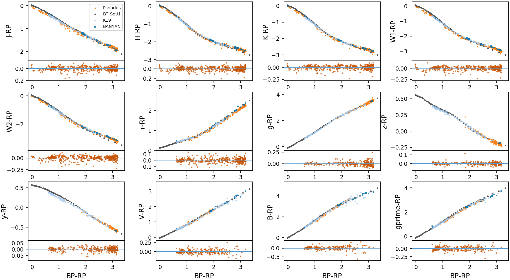
Figure 2: Color-color relations used in SED fitting (except $i$-band) for the set of Pleiades stars (orange dots), and young stars from Kounkel et al. (2019) (light blue dots) and BANYAN (Gagné et al., 2018; Gagné & Faherty, 2018) (deep blue square). Each relationship is shown in the color-color space (top panel) and the residual from a best-fit polynomial. The top panel includes a comparison with colors from BT-Settl spectra with $\log g=4.5$ (gray dots).

Table 2: Selected catalogs of Orion Stars

	Region	Disk ID
Fang et al. (2013)	L1640	Yes
Fang et al. (2017)	NGC 1980	Yes
Getman et al. (2017)	Orion A	Partial
	Orion B	Partial
	ONC	Partial
	Flame Nebula	Partial
Kuhn et al. (2013)	Flame Nebula	No
Megeath et al. (2012)	Orion A, B	No
Prisinzano et al. (2008)	ONC	Yes
Kounkel et al. (2019)	Orion A, B	Yes
	Orion A, B	Yes
	$\sigma$ Ori	Yes
	$\lambda$ Ori	Yes
	25 Ori	Yes

2.1 Building a Grid of SEDs of young stars

The photometric grid of young stars is built from Pleiades photometry. The samples that are described here cover from $BP-RP=3.2$ to $0$, corresponding to 3000 K to 9500 K. The cool end is sufficient for fitting bright brown dwarfs in Serpens.

The Pleiades members used for building grids are obtained from several catalogs. First, some Pleiades stars are collected from Cottaar et al. (2014), which focused on targets with temperatures of 3200–6000 K, as measured from H-band APOGEE spectra. For stars hotter than 6000 K, membership and temperatures are obtained from previous SED fits (Bouy et al., 2015; Barrado et al., 2016; Somers & Stassun, 2017; Bouvier et al., 2018); any hot star in our grid appears in at least two of those catalogs with an adopted temperature averaged from those catalogs. Stars cooler than 3200 K are identified from Gaia Collaboration et al. (2018) and assessed a temperature from the SED fitting method in Pecaut & Mamajek (2013), who used synthetic spectra to fit the SEDs of stars with negligible extinction. From these catalogs, we then ensure high confidence in membership by requiring that all stars are contained in a 5 pc sphere around the center of the full Pleiades population, in addition to proper motion constraints applied by Gaia Collaboration et al. (2018). The few Pleiades candidates with $BP-RP>3.2$ are faint and have large uncertainties in $BP$ photometry and are therefore excluded.

To obtain tight color-color relations, a polynomial is fit to the $BP-RP$ and $G-RP$ relationship. Stars with colors that are more than $2\sigma$ from the fit are removed. We iterate this process until the RMS of the $BP-RP$ and $G-RP$ relation is $<0.02$ mag. A similar procedure is applied to the relationship between $BP-RP$ and $M_{G}$. These stars form our initial grid for Pleiades (see color-magnitude and color-color diagrams in Figures 1– 2).

Due to saturation limits, only Pleiades stars with $T_{\rm{eff}}<4000$ K have Pan-STARRS photometry, while only those with 4000 K $<T_{\rm{eff}}<$ 6000 K have APASS photometry. To supplement our grid, we add young ($<300$ Myr old) stars within 1000 pc, collected from Kounkel & Covey (2019), Gagné et al. (2018), and Gagné & Faherty (2018). These samples are all expected to have roughly solar metallicities (Spina et al., 2017). To ensure negligible extinction and the lack of a circumstellar disk, these additional members are fitted only from Pleiades via the same method in Section 3 and are required to have: $|(BP-RP)_{\rm fit}-(BP-RP)_{\rm observed}|<0.06$, $\chi^{2}(\rm fit)<0.5$, and $A_{V}(\rm fit)<0.03$. The fitted result is presented in Appendix B. This total sample provides Pan-STARRS photometry for stars cooler than 7000 K, sufficiently covering the temperature range of most young stars.

2.2 Stars in Orion to test and apply the SED fits

To test the accuracy of our fitting methods, we apply our SED fits to stars in the Orion Star-forming Complex, leveraging the photometric and spectroscopic analyses by various catalogs (Table 2) that include an evaluation of disks from Spitzer mid-IR photometry. Temperatures are obtained from APOGEE spectra (Kounkel et al., 2018). Samples from catalogs in Table 2 are cross-matched with Kounkel et al. (2018) to ensure astrometric membership in Orion. Samples from Fang et al. (2013, 2017) are used to identify stars with and without disks (Section 3.5).

2.3 The sample of Serpens stars

The SED fits are designed to derive the stellar properties of the $\sim 700$ high-confidence members of the Serpens star-forming complex with Gaia DR2 astrometry (Herczeg et al., 2019). About half of the optical members are located in three distinct clusters, named Serpens Main ($\sim 440$ pc), Serpens Northeast (Serpens NE, $\sim 480$ pc) and Serpens far-South ($\sim 380$ pc). Of these clusters, Serpens Main is rich in protostars (Dunham et al., 2015), while the others have few protostars and disks. In addition, the Serpens South cluster is rich in protostars but has few optical counterparts. A few optical members of the Serpens cloud are located in smaller groups, and the rest are distributed throughout the complex. Among the $\sim 700$ high confidence members in Herczeg et al. (2019), $\sim 20$ stars have no Gaia $BP$ or $RP$ photometry, $\sim 20$ stars have no 2MASS data with a crossmatch radius of 2 arcsec, and $\sim 80$ stars do not pass the 2MASS data selection criteria, in most cases because the objects appear elongated by a companion or visual binary. Thus, over 100 stars are removed from the sample, leaving 569 stars for analysis.

2.4 Synthetic Spectra and filter profiles

Synthetic spectra are used for comparisons to observed color-color relations (e.g. Section 2.1) and for estimating the effect of surface gravity and circumstellar disk in SED fitting (Section 3.8). Synthetic spectra are obtained from BT-Settl models Allard et al. (2012) with solar abundances from Asplund et al. (2009). Filter profiles and zero points are collected from the SVO Filter Profile Service (Rodrigo et al., 2012; Rodrigo & Solano, 2020) for the following filter sets: GAIA/GAIA3 (GAIA eDR3 release), 2MASS/2MASS, WISE/WISE, PAN-STARRS/PS1, and Misc/APASS. The synthetic spectra from model atmospheres are used to assess the effects of surface gravity (see Section 3.8.1). More broadly, differences between the Pleiades colors and synthetic colors from the model spectra, as seen in Figure 2, demonstrate why the SED fitting requires empirical colors.

2.5 Pre-main-sequence Evolutionary Models

To estimate ages, we adopt the Feiden (2016) non-magnetic evolutionary models. For comparison, the magnetic isochrones from Feiden (2016) and the PARSEC isochrones (Bressan et al., 2012; Chen et al., 2014, 2015; Tang et al., 2014) are also used to evaluate uncertainties related to different models of pre-main sequence evolution.

3 Developing an SED fitting method

3.1 Overview

In our fitting method, we first create SEDs from the combination of temperature $T_{\rm{eff}}$, luminosity $L$, and extinction $A_{V}$ (Section 3.2) and then compare these SEDs with the observed stellar SED (Section 3.3). Since YSOs may contain a dusty accretion disk that affects the observed SED, we separately treat disk and diskless stars (Section 3.5). The fitting method is tested in Section 3.6 and compared with other fitting methods in Section 3.7. Caveats of this method are discussed in Section 3.8.

3.2 Generating SEDs

Pleiades stars are used to generate empirical SEDs with photometry in the following filters: $BP,RP,J,H,K,W1,W2,g,r,i,z,y,g^{\prime},B,V$. Figure 1 and 2 show relationships between colors, magnitudes, and temperatures for the Pleiades stars and young stars from other catalogs (see also additional color relationships in Appendix A). In general, young stars from these catalogs are consistent with Pleiades stars in color-color relations. Colors from BT-Settl spectra differ from Pleiades relations, especially at temperatures cooler than $\sim 4000$ K, as expected from previous assessments (e.g. Bell et al., 2012; Herczeg & Hillenbrand, 2015; Lançon et al., 2020).

First, colors in Figure 2 are reddened by visual extinction $A_{V}$ and relative extinction $A_{X}/A_{V}$, as obtained from the analysis of red clump stars with total-to-selective extinction coefficient $R_{V}=3.16$ (Wang & Chen, 2019) (except $BP$ and $RP$), and from Gagné et al. (2020) for Gaia $BP$ and $RP$. Extinction corrections are applied only for the Gaia $BP$ and $RP$ photometry, based on the temperature dependence determined by Gagné et al. (2020). Then, the reddened colors are added by $m_{RP}$, leading to the generated SEDs for use in our fits.

The extinction-corrected color $BP-RP$ from the best fit is converted to $T_{\rm eff}$ from the color-temperature relationship established from Pleiades stars (see the bottom panel of Figure 1). The APOGEE $T_{\rm eff}$ is preferentially adopted when available, despite systematic differences between the APOGEE scale and the color-temperature relationship of Pecaut & Mamajek (2013), as shown in Section 2.1 and the bottom panel of Figure 1 where the APOGEE $T_{\rm eff}$ of Pleiades stars only covers 3200-6000 K and differs from Pecaut & Mamajek (2013) $T_{\rm eff}$. The SED fit also solves for an apparent magnitude $m_{RP}$, which is then converted to luminosity using bolometric corrections (Section 3.3), the extinction, and the distance. The temperatures in our fits range from 3000–9500 K and extinctions range from $0<A_{V}<6$.

The broadband SEDs generated from the empirical color-color relations are then fit to the photometry (in mag) of each star.

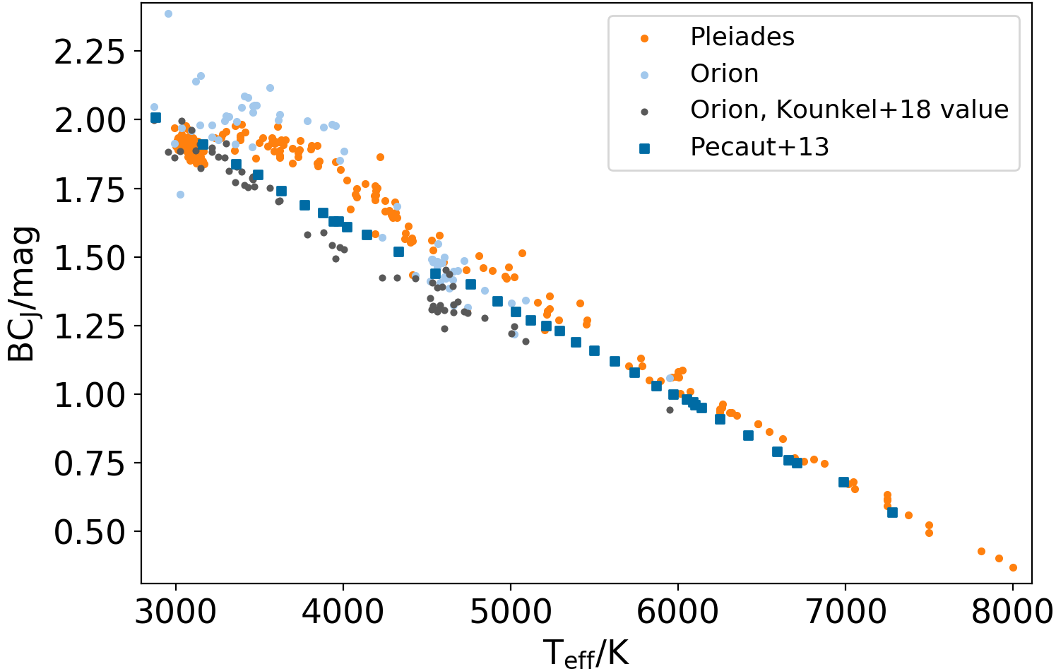
Figure 3: The relationship between the $J$-band bolometric correction and temperature directly from Pecaut & Mamajek (2013) in deep blue, the Pleiades APOGEE temperatures with bolometric corrections from Pecaut & Mamajek (2013) in orange, the Orion APOGEE temperatures with the Pecaut & Mamajek (2013) bolometric correction in light blue, and Orion APOGEE temperature with $BC_{J}$ converted from Kounkel et al. (2018) bolometric fluxes in gray.)

3.3 Fitting photospheric SEDs

In our fitting procedure, we find the minimum reduced $\chi_{\rm red}^{2}=\chi^{2}/(N-3)$, where $N$ is the number of data points, using the function scipy.optimize.minimize in python (Virtanen et al., 2019). The free parameters in the fit are an extinction-corrected $BP-RP$ (temperature), $A_{V}$ (extinction), and $m_{RP}$ (visual magnitude, converted to luminosity after extinction and bolometric corrections). Since these parameters have some degeneracies, the “minimize” function starts at 15 equally spaced locations of $BP-RP$ and 10 equally spaced locations of $A_{V}$.

For each photometric band, the uncertainty is estimated from a global evaluation of the average standard between the best-fit model and empirical measurement. The photometric uncertainty is first assumed to be $0.1$ mag to account for variability, unless the listed empirical error is larger than 0.1 mag. After fitting to all targets, the magnitude difference in all pass-bands is calculated. The standard deviation for each filter is then adopted as the magnitude uncertainty in the subsequent fitting process. We iterate one additional sequence to adopt final empirical uncertainties and measurements. Errors of the fitted parameters are calculated based on fits with $\chi^{2}-\chi^{2}_{\rm min}<3$ (Robitaille et al., 2007). Best-fit results at the edge of the fitting range are included in our tests (Section 3.6) but are excluded from any final results of Serpens members (Section 4.3).

The fits use as many of the photometric points as possible. However, as shown in Figure 2 (or Table 9) and described in Section 2.1, some photometry is only available over a limited range of $BP-RP$. For example, Pan-STARRS $g$ band photometry only exists at $0.8<BP-RP<3.2$, while APASS $V$ band photometry is available at $0.03<BP-RP<3$. Thus, when calculating $\chi^{2}$, $N$ will change with the input $BP-RP$, and a pass-band $X$ will not be used if the input $BP-RP$ exceeds the available $BP-RP$ range of pass-band $X$. Under these circumstances, a new minimum $\chi^{2}$ will be calculated for the relevant pass-bands in the previously fitted $BP-RP$.

The extinction-corrected $BP-RP$ of the best-fit SED is converted to temperature using the relationship determined from the Pleiades.

3.4 Bolometric corrections

The luminosity is calculated from $m_{RP}$, corrected for extinction and a $J$ band bolometric correction ($BC_{J}$) obtained for the relevant temperature from Pecaut & Mamajek (2013) for stars cooler than 7300 K. For hotter stars, the bolometric correction from $J$ band is obtained from PARSEC isochrones.

Since different $T_{\rm eff}$ calculation methods affect $BC_{J}$-$T_{\rm eff}$ relation, we compare $BC_{J}$-$T_{\rm eff}$ relations calculated from Pecaut & Mamajek (2013) $T_{\rm eff}$ and APOGEE $T_{\rm eff}$. For these comparisons, we with APOGEE $T_{\rm eff}$ include Pleiades stars (described in Section 2.1) and Orion stars (described in Section 2.2). The Orion stars are diskless stars with $A_{V}<=0.5$ and luminosities calculated by Kounkel et al. (2018)). Bolometric correction of these Orion stars via Kounkel et al. (2018) method is also included, where they derived bolometric flux from SED fitting and APOGEE $T_{\rm eff}$. The result ($BC_{J}$-$T_{\rm eff}$ relation) is shown in Figure 3, with the following results. When using APOGEE $T_{\rm eff}$ and Pecaut & Mamajek (2013) bolometric correction method, Pleiades and Orion relations overlap, with deviations at $\sim 4000$ K. Some of this difference maybe be caused by the discrepancy between APOGEE $T_{\rm eff}$ and Pecaut & Mamajek (2013) temperatures, as seen in the bottom panel of Figure 1.

3.5 Identifying stars with disks

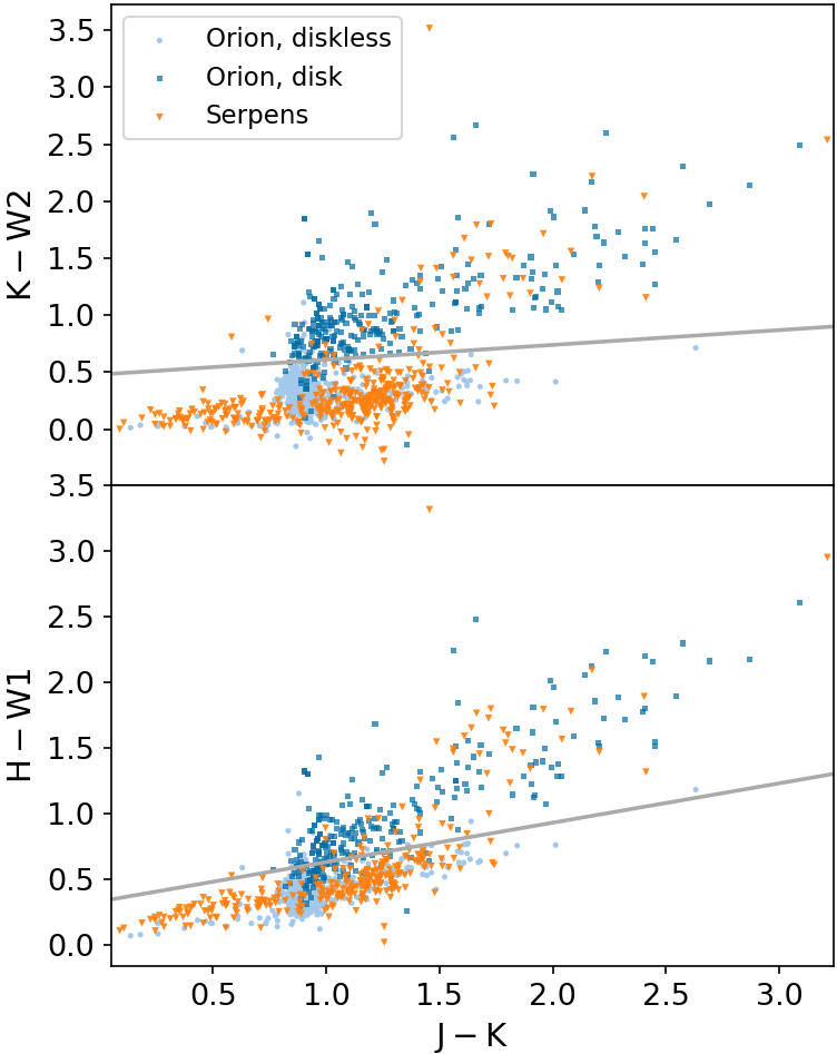
Figure 4: Color-color relationships to separate disk-hosting and diskless stars. In Orion, stars with disks (deep blue) and without disks (light blue) based on Spitzer photometry, separated by the solid gray line. Most optical members of Serpens (orange) are diskless stars.

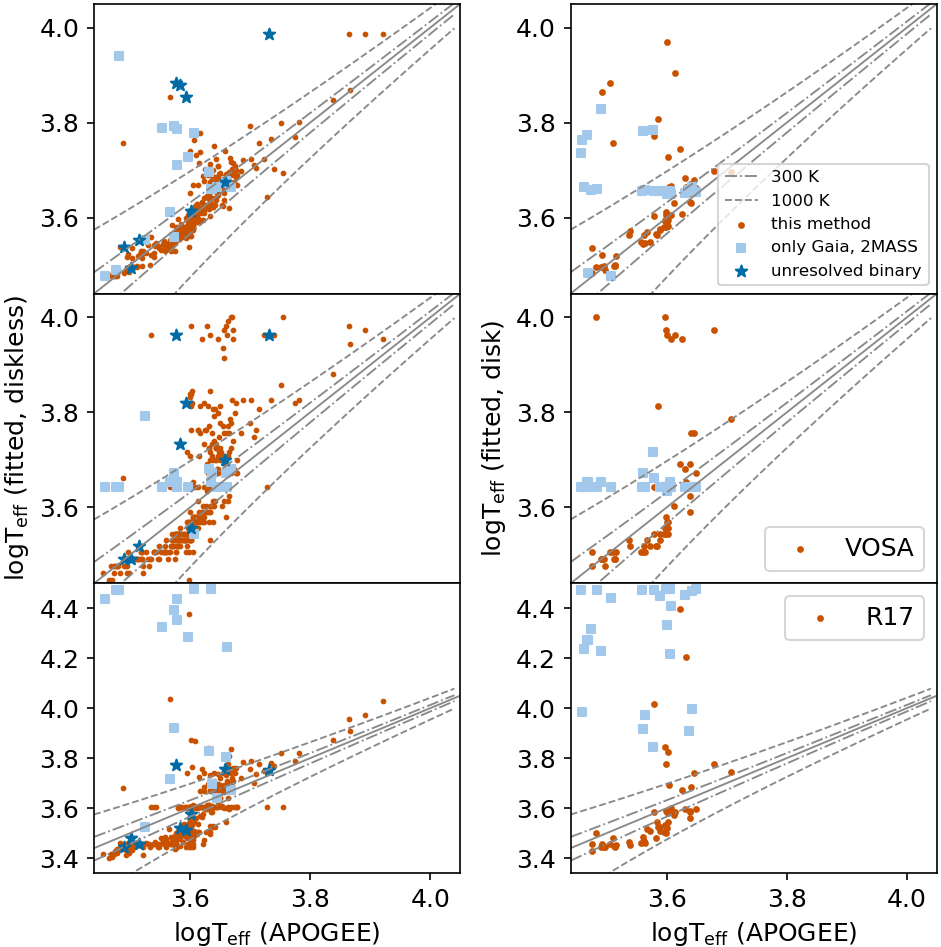
Figure 5: Comparison between temperatures from SED fits and literature (APOGEE) temperatures for diskless (left) and disk (right) stars in Orion, for our SED fitting method (top), VOSA (middle, Bayo et al., 2008), and Robitaille (2017) (bottom). The gray solid line represents equal temperature line, while gray dashed lines represent deviation of 300 K and 1000 K. The light blue square symbols are stars with only Gaia and 2MASS data in the fitting. The deep blue asterisk symbols are stars with a nearby source resolved by Gaia and within 2 mag in $G$ band, but unresolved by 2MASS.

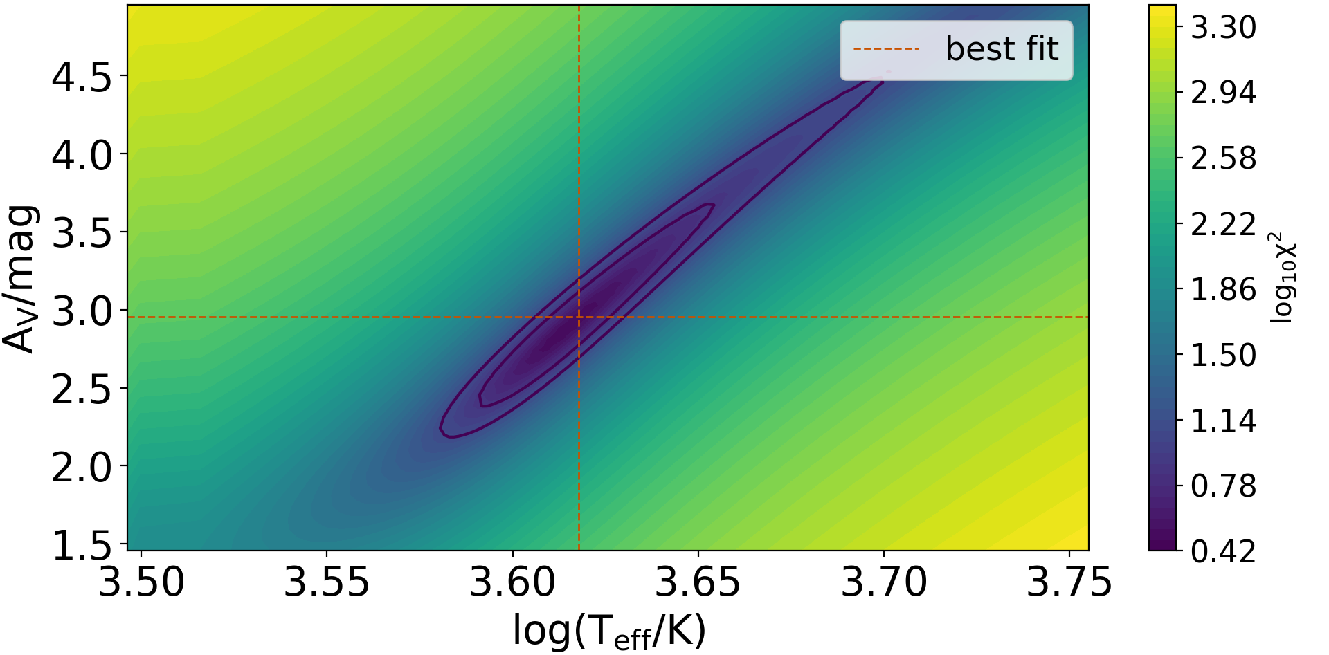
Figure 6: Contour of a diskless Orion star in the fitting calculated from grids of $T_{\rm eff}$ and $A_{V}$. Color bar represents $\log_{10}(\chi^{2})$. The black contours are $\chi^{2}-\chi^{2}_{min}=5$ and $\chi^{2}-\chi^{2}_{min}=10$. The orange lines are the best-fit $T_{\rm eff}$ and $A_{V}$.

The presence of a disk introduces complications to interpreting SEDs. Warm dust in accretion disks produce excess IR emission, especially in the all-sky WISE survey (see review by Williams & Cieza, 2011). Accretion produces excess H continuum emission that makes optical colors bluer, in some cases dominating over any photospheric emission (see review by Hartmann et al., 2016). For some viewing angles, the disk intercepts our line-of-sight to the star, so the observed emission from the star is extinguished and contaminated by scattered light. These processes are all variable (e.g. Grankin et al., 2007; Guo et al., 2018b; Venuti et al., 2021), which introduces additional uncertainties when comparing non-simultaneous data.

Figure 4 shows the 2MASS and WISE color-color relations used to separate disk and diskless stars, based on the identification of disks in the Orion sample from excess emission in Spitzer mid-IR imaging (Fang et al., 2013, 2017). To quantify the separation (Figure 4), we follow the “Class II box” method in Dunham et al. (2015) with disk and diskless stars separated by a line that maximizes the sum of the two kinds of probability: (a) the probability that a diskless star is located under the line (defined as the number of diskless stars under the line divided by the total number of diskless stars), and (b) the probability that a star under the line is classified as diskless (defined as the number of diskless stars under the line divided by the total number of stars under the line). Disks are identified from excess emission at $W2$, as seen in the $K-W2$ (or $H-W1$, if $W2$ photometry is unreliable) versus $J-K$. For stars with disks, $W1$ and $W2$ photometry are excluded from SED fits.

3.6 Testing the SED fitting results

To test the fitting method, we fit the SEDs of YSOs in Orion and then compare the resulting temperatures to those measured from APOGEE spectra (Cottaar et al., 2014; Kounkel et al., 2018). Fits to stars with and without disks are analyzed separately. We exclude stars that only have Gaia and 2MASS photometry and visual binaries that are resolved by Gaia and unresolved by 2MASS.

Figure 5 and Table 3 show the difference and scatter of fitted temperatures . In general, the difference and scatter of $T_{\rm eff}$ are 90 K and 433 K for stars without disks and 533 K and 1246 K for stars with disks. Our method is more reliable for both diskless and disk-hosting stars with $T_{\rm fit}<\sim$5000 K, where the difference and scatter are only -13 K and 208 K for diskless stars, and 53 K and 212 K for disk stars. For disk stars with higher fitted temperatures, the fit may be unreliable, affected by variability and by contamination of photospheric emission by emission from the accretion disk. Stars that only have Gaia and 2MASS photometry and also visual binaries that are resolved by Gaia and unresolved by 2MASS are included in Figure 5 to demonstrate that our method is not reliable for these stars. These stars are excluded in calculating the average temperature differences listed above.

Figure 5 also shows that there are more stars with $T_{\rm fit}-T_{\rm APOGEE}>300~{}K$ at $T_{\rm APOGEE}>\sim 4500~{}K\ (\sim 3.65$ dex) than at cooler $T_{\rm APOGEE}$, which is likely due to the larger degeneracy between $T_{\rm eff}$ and $A_{V}$ at higher temperature. Figure 6 shows the $\chi^{2}$ contours around the best-fit parameters for a diskless star, as calculated from grids of $T_{\rm eff}$ and $A_{V}$. The contours extend to high temperatures because of a large degeneracy between temperature and extinction. Such degeneracy is also shown in the bottom panel of Figure 7, where the color-color relation is closer to parallel with the extinction vector at higher temperature.

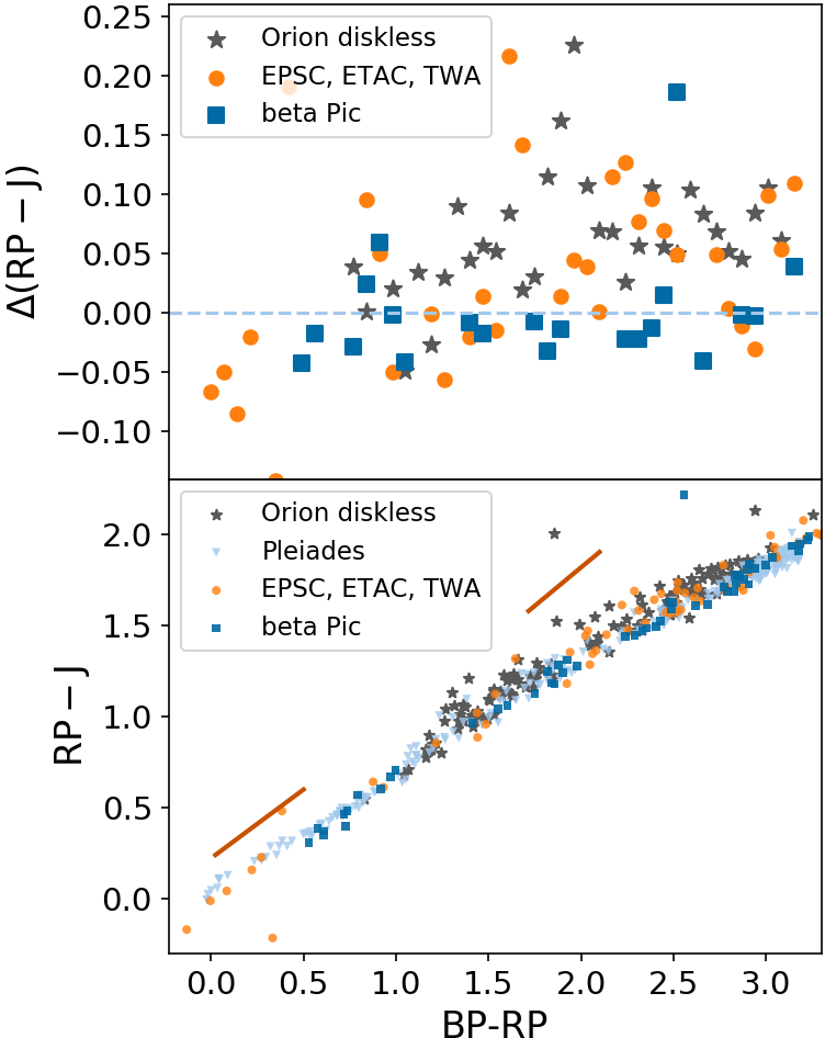
Figure 7: Color color diagrams (bottom) and residuals (top) for stars in groups with different ages. The Pleiades stars (light blue triangles) form the foundation for our fits, and are compared with diskless stars in Orion with $A_{V}<1$ (gray asterisk), the beta Pic Moving Group (deep blue square), $\epsilon$ Chamaeleontis, $\eta$ Chamaeleontis and TW Hya Association (orange). Deep orange line segments in the bottom panels are extinction vectors ($A_{V}=1$) at $BP-RP=0.5$ (left) and $BP-RP=2.1$ (right).

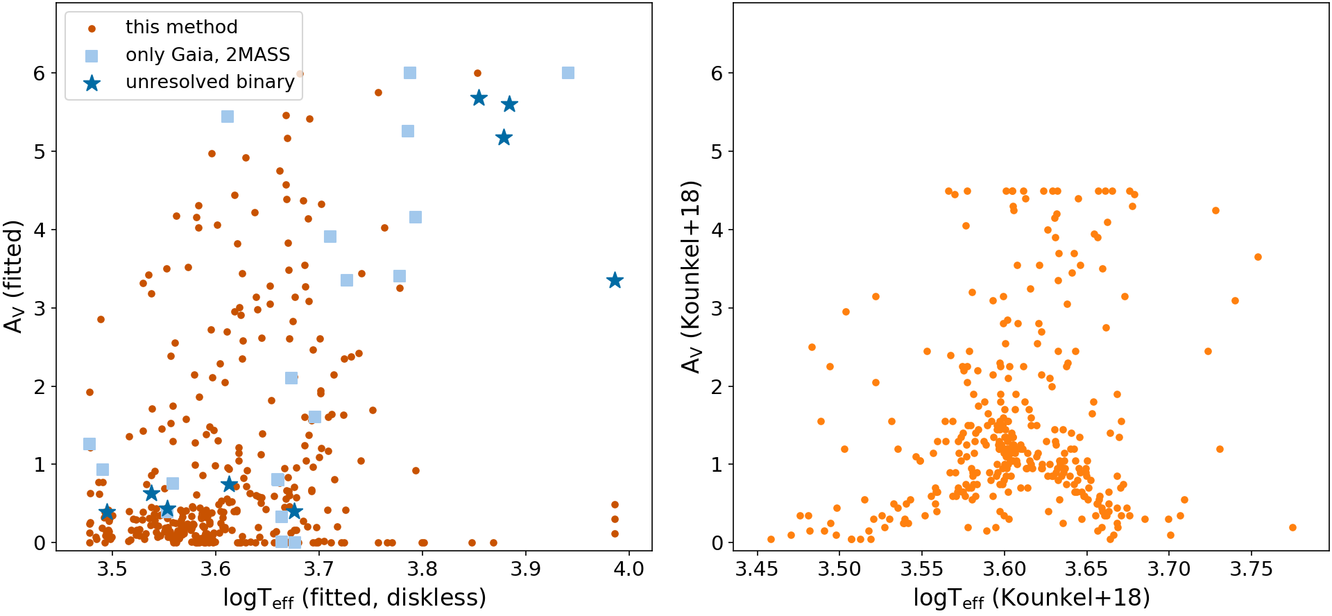
Figure 8: $T_{\rm eff}$ versus $A_{V}$ for diskless Orion stars, for (left) our results and (right) fits from Kounkel et al. (2018). The colors and symbols are the same as those in Figure 5.

Table 3: Temperature difference and scatter (in unit of K) between fitted and literature result for stars with the highest data quality .

$T_{\rm eff,fit}$ range (K)			Diskless			Disk
		this work	VOSA	R17	this work	VOSA	R17
<3500	Difference	-40	-323	-690	47	-194	-475
	Scatter	143	225	245	159	206	210
3500-4000	Difference	-129	-369	-431	-69	-344	-306
	Scatter	98	105	104	124	117	210
4000-5000	Difference	117	210	-21	186	392	605
	Scatter	240	436	389	234	246	199
>5000	Difference	857	2050	1565	3092	4114	5524
	Scatter	779	1474	2795	1350	1932	6366
All	Difference	90	380	-109	533	774	571
	Scatter	433	1324	1345	1246	1961	3331

Note. — The columns marked with “VOSA” and “R17” are comparison of VOSA and Robitaille (2017) SED fitting tools with details described in Section 3.6 and Section 3.7 separately.

Table 4: Average difference between model and observed magnitude

Region	disk	$T_{\rm eff,APOGEE}$	$\Delta g$	$\Delta B$	$\Delta BP$	$\Delta V$	$\Delta r$	$\Delta i$	$\Delta RP$	$\Delta z$	$\Delta y$	$\Delta J$	$\Delta H$	$\Delta K$	$\Delta W1$	$\Delta W2$
Orion	diskless	$<=4000$ K	0.13	0.3	0.02	0.10	0.08	0.03	0.03	0.01	0.02	0.03	0.03	0.02	0.03	0.04
		$4000-5000$ K	0.21	0.21	0.02	0.10	0.06	0.04	0.06	0.02	0.03	0.03	0.03	0.03	0.03	0.05
		$>5000$ K	0.16	0.20	0.01	0.08	0.05	0.05	0.03	0.01	0.03	0.04	0.02	0.02	0.03	0.05
		all	0.16	0.23	0.02	0.10	0.07	0.04	0.04	0.01	0.02	0.03	0.03	0.02	0.03	0.05
Orion	disk	$<=4000$ K	0.24	0.35	0.07	0.11	0.06	0.04	0.14	0.03	0.03	0.04	0.01	0.09	0.15	0.35
		$4000-5000$ K	0.47	0.21	0.07	0.07	0.18	0.08	0.17	0.05	0.05	0.08	0.04	0.15	0.15	0.34
		$>5000$ K	-	-	-	-	-	-	-	-	-	-	-	-	-	-
		all	0.39	0.22	0.07	0.07	0.10	0.05	0.15	0.04	0.03	0.05	0.02	0.10	0.15	0.34

Note. — Although the fitting on disk stars excludes $W1$ and $W2$, these pass-bands are still included in the table, representing the difference between model stellar photosphere SEDs and observed SEDs with infrared excess.

Note. — Only 1 disk star has $T_{\rm eff,APOGEE}>$5000 K, thus we do not report its magnitude difference.

Figure 8 shows the relationship between extinction and $T_{\rm eff}$ for diskless Orion stars from our results and from Kounkel et al. (2018). The distribution of extinctions in Kounkel et al. (2018) is $\sim 1$ mag higher for stars with $\log(T/K)\sim 3.6$ than for hotter and cooler stars, possibly due to differences between observed SEDs and synthetic spectra. Kounkel et al. (2018) first determined temperature from APOGEE spectra and then compared the observed SED with PHOENIX synthetic spectra (Husser et al., 2013) with the same $T_{\rm eff}$ to calculate $A_{V}$. If the stellar photosphere is redder than the synthetic spectrum, the calculated $A_{V}$ will be higher, leading to a gap in $T_{\rm eff}$ - $A_{V}$ relation (perhaps caused by the discrepancy seen in color-temperature scale in Figure 1). Such a gap is not seen in our fitting method (Figure 8, left panel), which is consistent with Orion stars having colors that are more similar to the Pleiades SEDs than to synthetic spectra.

Table 4 lists the average difference between fitted and observed magnitude of these Orion stars after two iterations of SED fits. In general, for diskless stars, the average magnitude difference is less than $\sim 0.03$ mag at pass-bands redder than $RP$. The larger uncertainties in blue wavelengths (except $BP$) are likely introduced by differences in spot coverage and by variability. For disk stars, the smallest average magnitude difference is at $H$ band. The $W2$ band, which is excluded in these fits, shows the largest difference, as expected for stars with excess infrared emission from disks. Optical pass-bands $BP$ and $RP$ have larger differences than the near-infrared passbands, likely because accretion variability and disk obscuration affect the optical more than the near-IR.

Additional descriptions and comments of these results are provided in Section 3.8.

3.7 Comparing our SED fits to other fitting methods

To compare with other SED fitting methods, photometry of stars in Orion are fit with the commonly used SED codes VOSA (Bayo et al., 2008) and Robitaille (2017) (hereafter Robitaille). Our fits with VOSA use the BT-Settl models with solar metallicity and surface gravity $\log(g)=4.5$, an extinction law from Fitzpatrick (1999) and improved by Indebetouw et al. (2005) in the infrared. The Robitaille fits use their “s—s-i” models (pure stellar photosphere models constructed from Castelli & Kurucz (2003) above 4000 K and PHOENIX atmospheres (Brott & Hauschildt, 2005) below 4000 K) with an extinction law consistent with $R_{V}=5.5$ (following the description in Forbrich et al., 2010).

Figure 5 and Table 3 show that the difference and scatter between the fitted and literature (spectroscopic) temperatures are 380 K and 1324 K for VOSA, -109 K and 1345 K for Robitaille (2017), and 90 K and 433 K for our method. All three methods are less reliable for stars that have only Gaia and 2MASS photometry and visual binaries that are resolved by Gaia and unresolved by 2MASS. In addition, at $\log T/K<3.6$, both the VOSA and Robitaille fits underestimate temperatures by $\sim$300 K to $\sim$1000 K relative to literature values. Both models also assess a wide range of temperatures for stars with spectroscopic temperatures of $\log T/K\sim 3.65$. In comparison, temperatures from our fits follow the literature estimates within $\sim 300$ K until $\log T/K=3.65$, where our models suffer from a similar but less severe dispersion. Possible reasons for this feature are discussed in Section 3.8.

In these comparisons, the stellar magnitude and fitting ranges are the same as Section 3.6. The Robitaille (2017) fits do not include additional temperature constraints, thus the fitted temperature can exceed the ranges of our method. Magnitude uncertainties are 0.1 mag in both VOSA and Robitaille (2017) fits, with no iteration executed in their methods.

3.8 Shortcomings and challenges in our SED fitting

This SED fitting method uses Pleiades stars to create templates to fit YSOs in the Serpens Molecular Clouds. However, the Pleiades stars are not perfect templates. Shortcomings caused by Pleiades include differences in surface gravity and spots (see Section 3.8.1). In addition, we comment on our fits to disk stars in Section 3.8.2, and show how positive extinction affects the fitting result on low extinction clusters (Section 3.8.3). Finally, we comment the outliers of the fitting result in Section 3.8.4.

3.8.1 Temporal evolution of color-color relations

Differences in color-color relations between Orion and Pleiades, perhaps caused by differences in gravity or spots, may lead to biases in the fitting result. In this subsection, we first give an example on how the difference in color-color relation influences the fitting result. We then discuss the effect of surface gravity and spots separately.

Figure 7 shows $(BP-RP)$-$(RP-J)$ for Pleiades, Orion, and members of the beta Pic Moving Group, $\epsilon$ Cha association, $\eta$ Cham association, and TW Hya Association from Gagné et al. (2018); Gagné & Faherty (2018). To quantify $(RP-J)-(RP-J)_{\rm Pleiades}$ at a given $BP-RP$, $(RP-J)-(RP-J)_{\rm Pleiades}$ is given by setting several bins in $BP-RP$ and calculating the average $RP-J$ in each bin that includes a star.

The $RP-J$ versus $BP-RP$ colors of the groups differ at $BP-RP\sim 2$ ($\sim 4000$ K or 3.6 dex), which may explain the temperature deviation in Figure 5. As a simple example, only $BP$, $RP$, and $J$ pass-bands are used in the following demonstration. First, a star in Orion with $A_{V}\sim 0$ mag, $BP-RP=2.15$ ($\sim 4000$ K or 3.6 dex) and $RP-J=1.62$ is selected. According to the Pleiades color-color relation and extinction vector in Figure 7, the fitted $BP-RP$ of this star is 1.32 ($\sim 4800$ K or 3.68 dex). While the fitted temperature is higher, the fitted extinction is also higher, leading to a gap in $T_{\rm eff}$-$A_{V}$ relation at $\sim 4000$ K. Although this is a simple demonstration using only three pass-bands, redder Orion stars may be one of the reasons for the temperature bump in Figure 5.

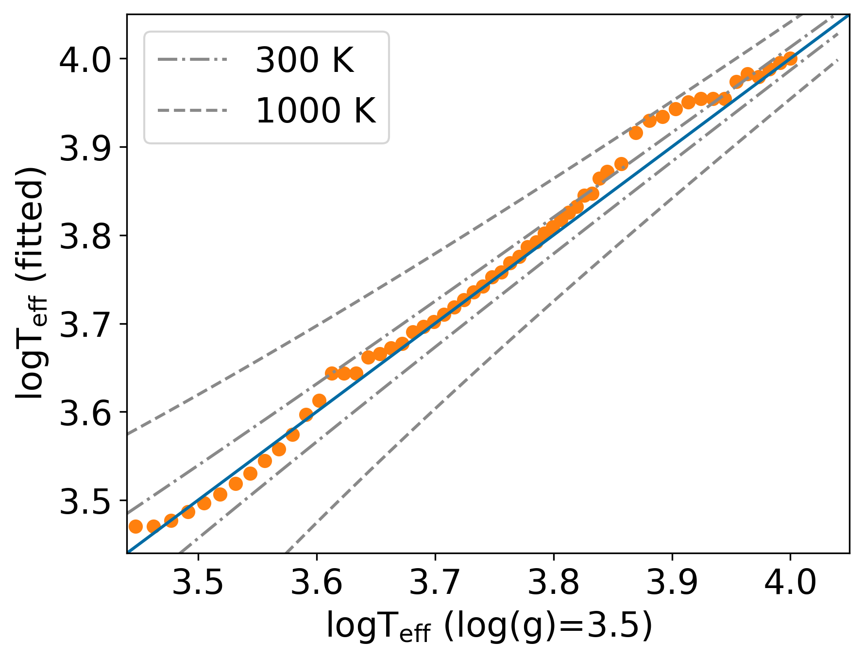
Figure 9: Comparison between temperatures for spectra with $\log g$ =3.5 and temperatures from fits to those spectra using $\log g$ =4.5 spectra as templates.

These colors may be caused by the increase in surface gravity as a star contracts, with empirical measurements from APOGEE of $\log(g)\sim 4.0$ for 2-6 Myr IC 348 stars to $\sim 4.8$ for $\sim$110 Myr Pleiades stars (Cottaar et al., 2014). To simulate the effect of surface gravity, we use BT-Settl models to describe that the lower gravity of younger stars leads to a higher fitted temperature at $\sim 4000$ K.

BT-Settl spectra with $\log g$ =4.5 are used to build basic SEDs as templates, while BT-Settl spectra with $\log g$ =3.5 are then used as the targets to be fitted. Offsets in Figure 9 (lower $T_{\rm fit}$ at $\sim$3.55 dex and higher $T_{\rm fit}$ at $\sim$3.61 dex is consistent with the similar offset in Figure 5. The offset at $3.6<\log{T_{\rm{eff}}}<3.7$ in Figure 5 is at least partially attributed to the difference in surface gravity.

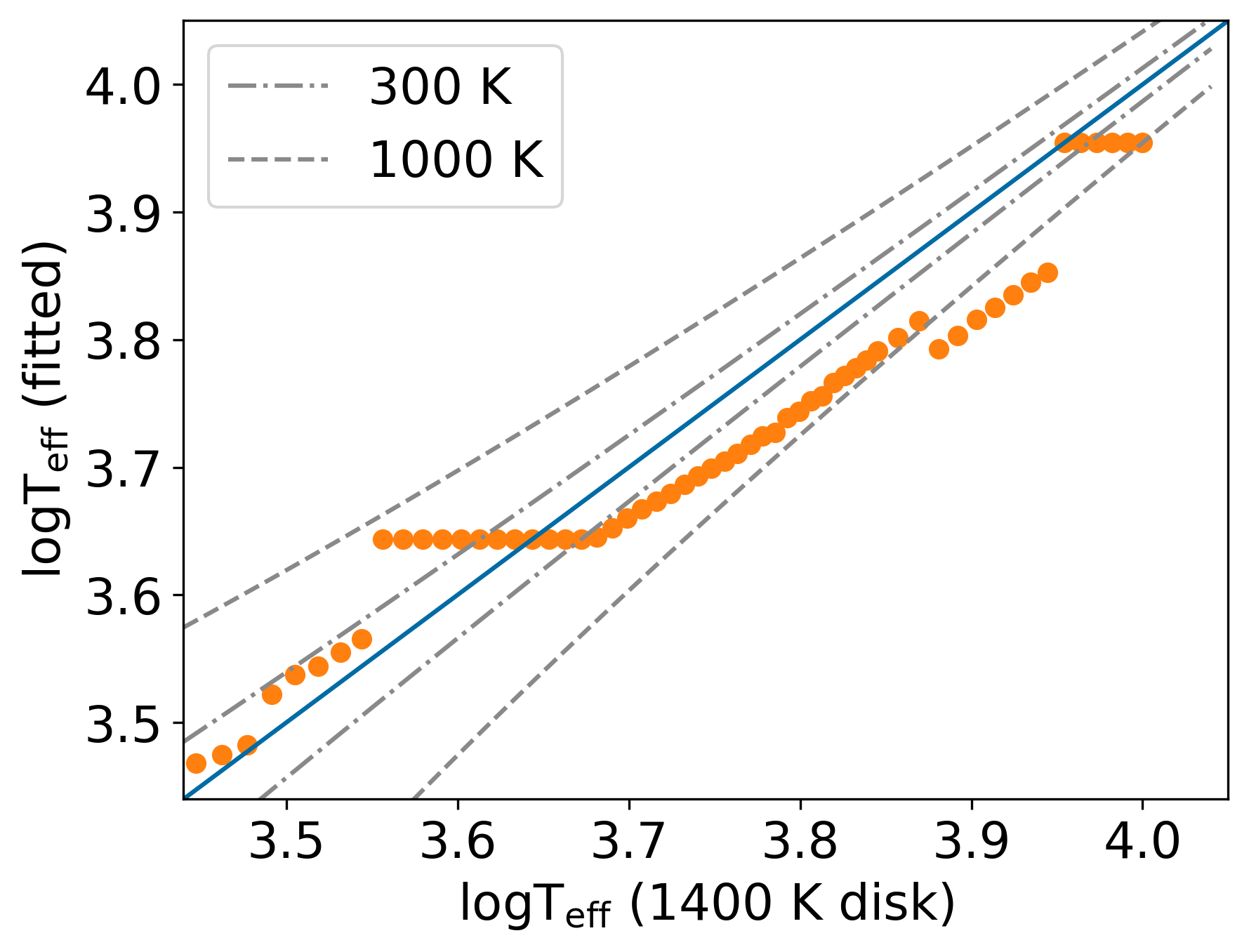
Figure 10: Comparison between the temperature of a BT-Settl spectra versus the fitted temperature of the spectrum plus a warm dust dusk.

In addition to surface gravity, spot properties also vary among YSOs (e.g., Grankin et al., 2008) and influence SED fitting result. Spots on magnetically active cool stars redden the broadband SED (e.g. Somers et al., 2020), leading to errors when fitting with single temperatures (Gully-Santiago et al., 2017). Although the Pleiades stars are heavily spotted (e.g. Stauffer et al., 2003; Fang et al., 2016; Guo et al., 2018a), our SED fits may be insufficient in incorporating spots, if they are more important for young stellar objects (Grankin et al., 2008).

3.8.2 Fits to disk stars

Stars with disks are not well described through photometric fits. Removing a few photometric points may avoid the influence of infrared excess and/or bluer optical colors caused by a disk, but enough pass-bands are still needed to constrain the photospheric properties. Most fitting routines, including ours, do not incorporate accretion, which alters colors and in some cases dominates the optical emission (e.g. Gahm et al., 2008). In such cases, any attempt to measure stellar properties from SEDs or spectra is dubious. More typical accreting stars, where the accretion flow affects but does not dominate the optical emission, have SEDs that are roughly simulated by models but are expected to show excess blue emission.

We evaluate uncertainties caused by emission from dust by creating SEDs from a combination of BT-Settl spectrum of the photosphere and a 1400 K blackbody for the dust, chosen as the dust sublimation temperature. The blackbody emission flux is scaled so that the $K$-band flux from the blackbody is two times of the photosphere flux (consistent with the ratios in Fischer et al., 2011). The spectrum is then fit with the BT-Settl spectra alone, excluding $W1$ and $W2$. The SED templates are based on interpolating BT-Settl color-color relations. The temperature comparison (Figure 10) shows that an offset of $\sim 1000K$ is present for stars at $\log T_{\rm eff}\sim 3.55$, while for the cooler stars the offset is smaller.

Although this simple approach indicates that the fits are robust to the presence of steady dust disks, the effect of disks are expected to be more significant than described here. In some cases the disk will obscure the star. Accretion from the disk onto the star contributes and in some cases dominates optical colors. Both disk obscuration and accretion are variable. These phenomenon are significant confounding factors that are not explored in this paper.

3.8.3 Fits to the Pleiades and constrained extinctions

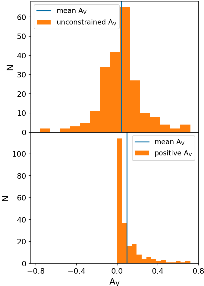
Figure 11: The distribution of best-fit $A_{V}$ (orange histogram; mean indicted with the blue line) of Pleiades stars, for fits that are unconstrained by reality and allowed to be negative (top panel) and fits that are constrained to be $\geq 0$ (bottom panel).

The extinction range ($0\leq A_{V}\leq 6$) affects the extinction distribution of a cluster with low extinction and statistical comparisons of low-extinction clusters to high-extinction clusters. Figure 11 shows the best-fit $A_{V}$ to stars in the Pleiades. The average $A_{V}$ is 0.04 mag when $A_{V}$ is allowed to be negative and 0.1 mag when $A_{V}$ cannot be negative. The spread in estimated $A_{V}$ and therefore the size of this effect is likely larger for younger stars.

3.8.4 Outliers in the temperature comparison

In this subsection, we comment on stars with the best-fit SED temperature deviating by 1000 K from the previously measured literature temperature, with a total number of 13 stars after excluding those with photometric issues in Section 3.6:

For the four stars in this small sample with Pan-STARRS photometry, three are saturated in the $z$ band. Since $z$ band has the largest weight among the magnitudes when fitting SEDs (Section 3.3, Table 4), the saturated z-band photometry has a significant influence on the fitting result. The fourth star has a $g$ band image where the star appears to fall at the edge of the detector.

Six stars are variable stars reported by ASAS-SN (the All-Sky Automated Survey for Supernovae, Shappee et al., 2014; Kochanek et al., 2017), with amplitudes from 0.1 mag to 0.3 mag. A seventh star has not been reported as a variable star but shows a wavy light curve with an amplitude of $\sim 0.1$ mag.

The previous two sets of stars have some overlap. Of the remaining stars, three with the highest $T_{\rm fit}$ have $A_{V}(\rm fit)<0.5$, indicating a higher degeneracy between $T_{\rm eff}$ and $A_{V}$, which is due to the extinction vectors becoming more parallel to color-color relations at higher temperature, as shown in the bottom panel of Figure 7. Two stars are not explained by the above descriptions.

Table 5: Fits of Serpens members

Gaia EDR3 ID	RA/deg	DEC/deg	Region	d/pc	Teff/K	$A_{V}$	$L$(log$L/L_{\odot}$)	Age/Myr	Mass/$M_{\odot}$	Disk	Flag
4309522600884785536	289.69099	10.80327	LDN 673	376	7014	0.84	0.69	21.8	1.50	-	1
4309648735482263936	290.35284	11.11158	LDN 673	414	4401	2.58	0.15	1.9	1.02	0	0
4309847540917708416	290.04547	11.3505	LDN 673	409	3013	2.03	-0.51	1.0	0.18	0	0
4309847884515108480	290.01491	11.37616	LDN 673	406	3743	2.03	-0.67	6.0	0.56	-	1
4271424759186100352	275.28395	-1.30382	Distrib	430	4282	1.90	-0.10	2.6	0.86	0	1
4271223720358239744	275.73095	-1.40617	Distrib	369	4322	0.28	-0.91	47.8	0.68	0	1
4271528250719881728	275.50849	-1.08444	Distrib	443	3005	1.29	-1.35	3.8	0.09	0	0
4269964371522804224	275.3711	-2.62225	Distrib	449	4526	0.00	-0.50	21.8	0.88	0	1
4269965196156468480	275.51853	-2.60617	Distrib	456	4215	0.12	-0.66	22.9	0.82	0	1
4270725160552584960	275.46313	-2.40182	Distrib	446	4157	0.80	-0.98	47.8	0.66	0	1
All photometry in a table for vizier

Note. — ”Flag”: ”0” represents that this star is not included in calculating cluster ages (Section 4.3). Individual distances are adopted from Gaia EDR3 parallaxes.

4 SED Fits to Members of the Serpens Star-forming regions

The primary motivation for this paper is to characterize the optically bright stars in Serpens. Of the previously identified optical members in Serpens, 569 stars pass the photometric selection criteria and have SEDs fit here. To analyze their SEDs, the first step is identifying if a star has a disk (Section 4.1). The SEDs are fit to the relevant bandpasses, with results and analysis presented in Section 4.2. We then analyze the cluster ages in Section 4.3.

4.1 Disk Presence

The presence of disks around young stars is typically assessed from mid-IR photometry. Since much of the Serpens cloud was imaged by Spitzer, we first cross-match the Serpens sample with Spitzer catalogs (Evans et al., 2003; Gutermuth et al., 2008; Dunham et al., 2015) and find 123 stars with Spitzer data. A disk is determined to be present in 52 stars based on an IR spectral index $\alpha>-1.6$, following Dunham et al. (2015). For the Serpens stars without Spitzer data, disk presence is identified by WISE and 2MASS color cuts (Figure 4). In total, there are 359 diskless stars (71 from Spitzer, 288 from 2MASS and WISE colors as seen in Figure 4), 86 disk stars (52 from Spitzer, 34 from WISE), and 231 stars without disk information due to the lack of both Spitzer data and reliable WISE data.

To confirm consistency in assessing disk presence or absence, we evaluate 82 members with both Spitzer and WISE photometry. Applying these color cuts to regions imaged by Spitzer show that the methods are mostly consistent. The 10% of stars that change classification between disk and diskless, all located near the borders of the classification system. To avoid the appearance of disk stars in fitting diskless stars, stars that have both WISE and Spitzer photometry are treated as diskless only if both sets of measurements indicate the lack of disk.

Disk properties from Figure 4 are evaluated from the results of SED fits to Serpens members. The fitted $W1$ and $W2$ magnitudes are compared with observed magnitudes to evaluate the disk selection in Figure 4. We would then reclassify the presence of a disk if the $W1$ or $W2$ magnitude is at least $0.78$ mag or $0.98$ mag (the average magnitude difference of disk stars) above the photospheric level, while disk stars would be re-classified as diskless if the $W1$ and $W2$ magnitude are less than $0.05$ mag and $0.09$ mag (the average magnitude difference of diskless stars) of the photospheric level. In this reassessment, only one star is reclassified into the diskless category, and all stars previously identified as diskless remain diskless. We update results following this possible reclassification.

4.2 Isochrone fits to stellar properties

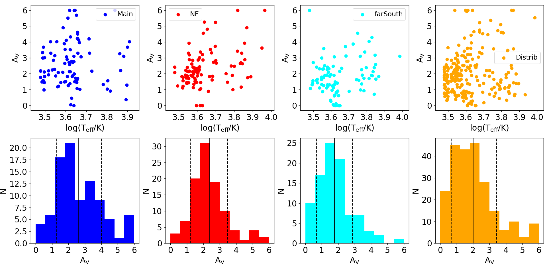
Figure 12: Temperature versus extinction (top panels) and the distribution of extinctions (bottom panels) for four major groups in Serpens. The black lines in bottom panels are the mean and standard deviation of $A_{V}$.

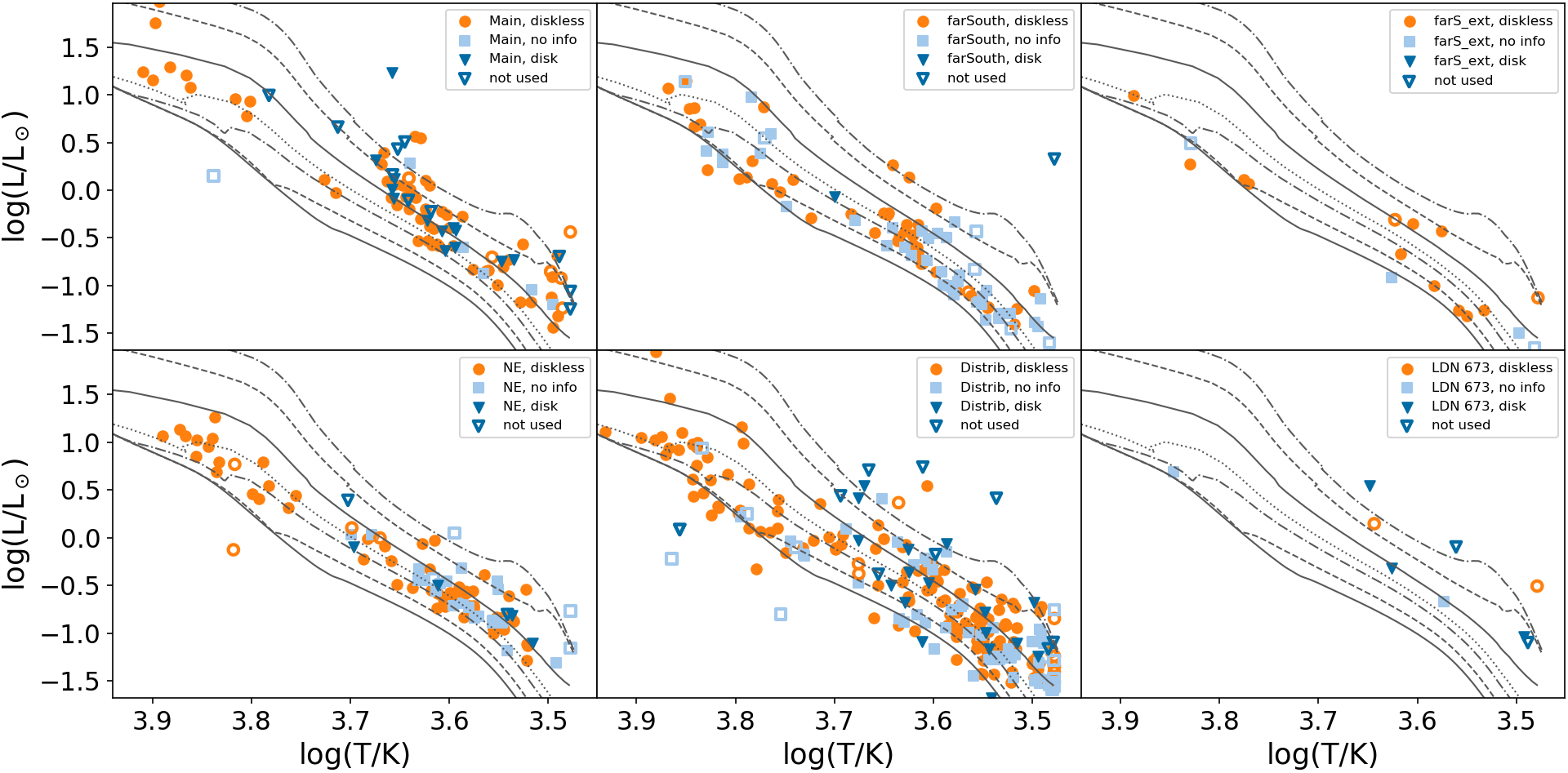
Figure 13: The HR diagram of Serpens members in different groups, compared with isochrones from the non-magnetic evolutionary tracks of Feiden (2016), for stars with disks (deep blue triangles), without disks (orange dots), and without disk information (light blue squares). Unfilled symbols are stars which are not used in calculating ages. The gray curves are isochrones with 1 Myr, 2 Myr, 5 Myr, 10 Myr, 15 Myr, 30 Myr, 50 Myr from top right to bottom left.

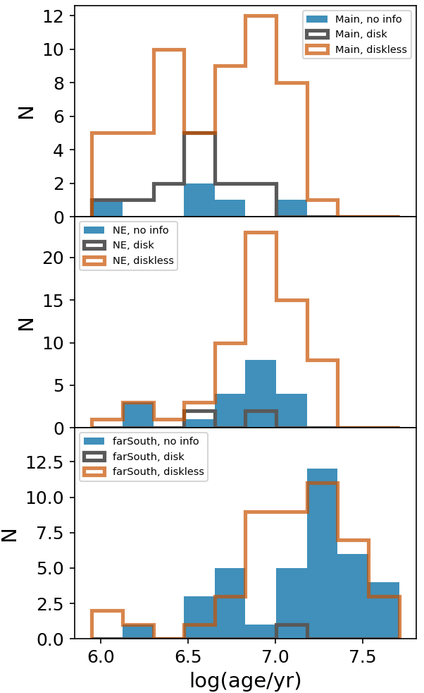
Figure 14: The distribution of ages for three groups in Serpens: Main (top panel), NE (medium panel) and far-South (bottom panel), in order of average age for the group. The age spread in each group may not be significant (see discussion in Soderblom et al., 2014).

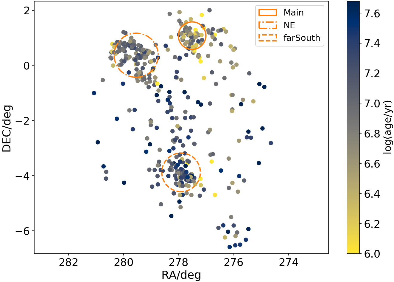
Figure 15: Spatial location of Serpens members with colors mapped by ages. Orange circles represent the location of three subgroups: Serpens Main, NE and farSouth, with location and radius adopted from Table 1 of Herczeg et al. (2019).

Table 5 presents the best fit temperatures, luminosities, and extinctions for stars associated with the Serpens Molecular Cloud. Figure 12 shows color excesses due to extinction versus temperature for stars in four different regions in Serpens (Main, NE, far-South, Distributed). The optical members of Serpens Main have the highest median extinction, while Serpens far-South is the least extincted, consistent with Serpens Main hosting more ongoing star formation than Serpens far-South.

The masses and ages of individual stars are determined by comparing the temperature and luminosity to pre-main sequence evolutionary models for non-magnetic stars calculated by Feiden (2016), using the isochrone fitting method in Zari et al. (2019). Specifically, the likelihood for a single star to come from an isochrone with an age of $\tau$ is

$$L(\tau)=\int L(\tau,m)dm,$$ (1)

where $m$ is the mass of a point in the isochrone, and $L(\tau,m)$ is calculated from

$$L(\tau,m)=\frac{1}{(2\pi)^{1/2}\sigma_{T}}\frac{1}{(2\pi)^{1/2}\sigma_{L}}\exp{(-\chi^{2}/2)},$$ (2)

with:

$$\chi^{2}=\left(\frac{T-T_{iso}}{\sigma_{T}}\right)^{2}+\left(\frac{Lum-Lum_{iso}}{\sigma_{Lum}}\right)^{2},$$ (3)

where $T$, $Lum$, $\sigma_{T}$, $\sigma_{L}$ represent temperature, luminosity and their errors (in log scale) of a star, while $T_{iso}$ and $Lum_{iso}$ are temperature and luminosity of a point in an isochrone which are determined by mass and age. The maximum $L(\tau)$ corresponds to the best-fit age. The isochrone fitting procedure is based on linear space of the isochrones.

4.3 Age estimates for Serpens subclusters

In this section, ages are estimated via different isochrones and different methods. Stars with photometric problems or with best-fit parameters at the edge of the parameter space of our grid (Section 3.6) are excluded in calculating ages, with a total number of 455 stars used in age estimation. The ages adopted in this study is derived in section 4.3.1, while the comparison of ages are presented in Section 4.3.2

4.3.1 Ages adopted in this study

Table 6: Ages and errors (Myr) of Serpens groups with non-magnetic isochrones

	disk	error	diskless	error	total	error	disk fraction
Main	3.0	0.5	4.0	0.2	4.0	0.2	0.22
NE	7.6	2.9	8.3	0.3	8.3	0.3	0.03
farSouth	9.5	9.3	11.5	0.4	13.8	0.9	0.04
farS_ext	-	-	21.9	1.6	21.9	1.4	0.00
FGAql	-	-	-	-	-	-	-
LDN673	2.9	0.5	-	-	6.3	1.4	-
Distrib	5.5	0.6	10.0	0.3	10.0	0.4	0.12

Note. — Estimated with isochrone fitting. Total includes disk and diskless, and sources with no disk information.

Table 7: Ages and errors (Myr) of Serpens groups with different isochrones and different estimation methods

	Feiden, standard		Feiden, magnetic		Feiden, magnetic		PARSEC		PARSEC		PARSEC
	$T_{\rm eff}-L$		$T_{\rm eff}-L$		$T_{\rm eff}-L$		$T_{\rm eff}-L$		$T_{\rm eff}-L$		CMD
	Cool stars		All stars		Cool stars		All stars		Cool stars		Cool stars
Region	age	error	age	error	age	error	age	error	age	error	age	error
Main	4.0	0.3	7.9	0.2	9.1	1.0	4.0	0.2	4.8	0.5	7.2	0.3
NE	6.9	0.5	17.4	0.5	18.2	1.6	7.9	0.3	7.6	0.5	9.1	0.3
farSouth	13.2	1.5	31.6	0.9	26.3	3.0	13.8	0.8	20.0	2.0	19.0	0.6
farS_ext	9.5	3.3	34.7	2.0	20.0	6.2	22.9	2.3	15.1	4.5	25.1	1.9
FGAql	-	-	-	-	-	-	-	-	-	-	-	-
LDN673	3.8	2.1	15.1	0.7	11.5	5.3	6.3	1.3	6.6	2.0	4.8	0.3
Distrib	6.6	0.5	22.9	0.5	15.8	1.0	10.0	0.3	10.0	0.6	10.5	0.3

Note. — Estimated with isochrone fitting.

Note. — $T_{\rm eff}-L$: Ages are estimated in temperature-luminosity space. CMD: Ages are estimated in color-magnitude diagram (Pan-STARRS $r-i$ versus $r$).

Note. — Cool stars: Stars with $r-i>1.2$ ($\sim 3500<T_{\rm eff}<\sim 4500K$).

The ages adopted in this paper are determined by comparing Feiden (2016) non-magnetic isochrones to the temperature and luminosity of each source, adopting individual stellar parallax distances for each star (see Figure 13. Table 6 lists the ages and errors of different groups within the cloud, as calculated from isochrone fitting. For the major groups in the cloud, Serpens Main is assessed an age of 4 Myr, Serpens NE is 8.3 Myr, Serpens far South at 13.8 Myr, and the extended group of far-South (labeled as farS_ext) is 21.9 Myr. The small LDN 673 Group age of 6.3 Myr is calculated from 5 stars and is therefore not well constrained. Serpens South and W40 are deeply embedded and lack sufficient optical members for age estimates, but they are presumably younger than Serpens Main.

Figure 14 shows the age distribution of Serpens Main, Northeast and far-South. To check if age distributions within a single subcluster are significant (see Figure 14), age errors of individual stars are calculated via the method in Zari et al. (2019) by adopting the 16th and the 84th percentiles of the likelihood (Equation 1) distribution. The average age error is $\sim 0.2$ dex. Since the error relies on temperature and luminosity errors from SED fitting, which are limited by fitting ranges (Section 3.6), the $\sim 0.2$ dex age error does not reflect the real age probability distribution. Although some age spread within clusters is likely, it is unclear from our current methods and analysis whether we could subdivide any group according to age. Adopting single distances for each cluster does not significantly change the age but would change individual stellar ages.

Figure 15 shows a map of members of the Serpens star-forming region, with stars colored by age. Age difference among subgroups (Figure 14 and Table 6) is also indicated by Figure 15. The youngest subgroup, Serpens Main, is the smallest and densest group, as shown in Figure 15, while the oldest stars are scattered in the distributed region.

4.3.2 Ages from other estimation methods

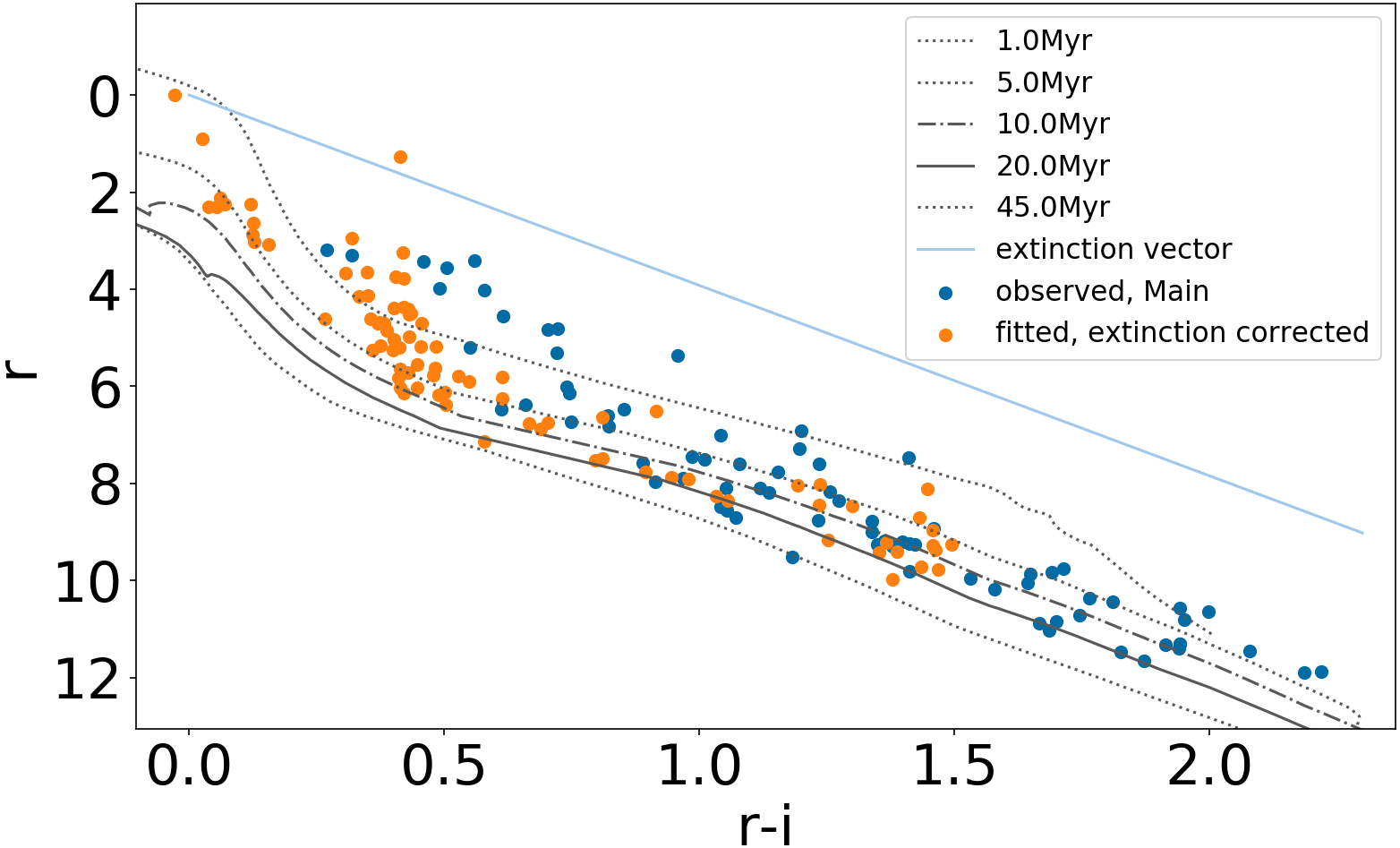
Figure 16: Color-magnitude diagram for Pan-STARRS $r$ versus $r-i$, with PARSEC isochrones (gray curves), with stars in Serpens Main (blue and orange dots represent the same set of stars with observed and extinction corrected result separately), and the extinction vector (light blue straight line) that runs parallel to the isochrones for cool stars.

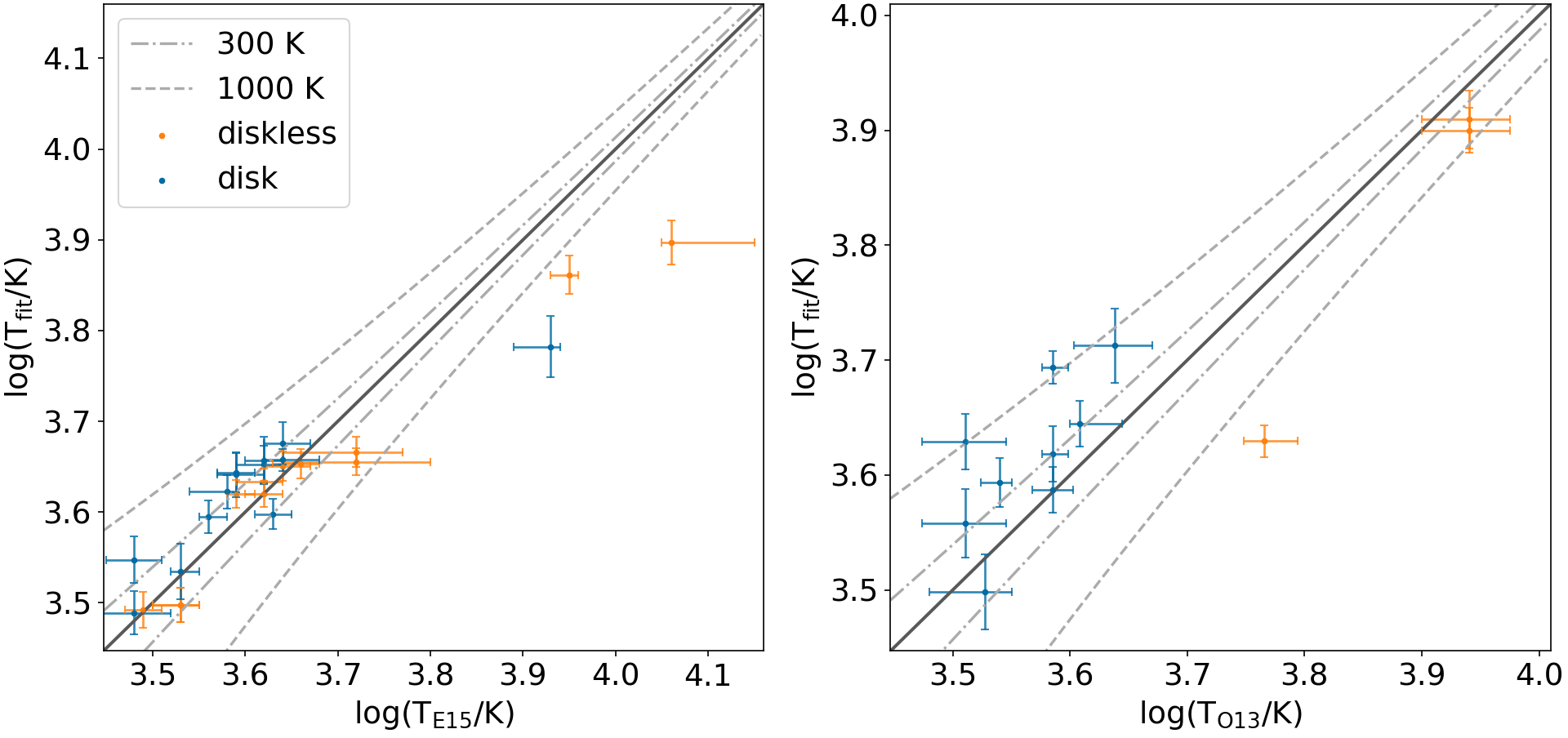
Figure 17: Comparison between temperatures derived in this paper and in Erickson et al. (2015) (left) and Oliveira et al. (2013) (right). Orange symbols are diskless stars, and blue symbols are disk stars.

The age estimates are sensitive to evolutionary tracks and to the method for isochronal fitting. In this section, we explore systematic uncertainties in the ages due to the methodological choices.

Table 7 compares ages from the non-magnetic and magnetic Feiden (2016) and from PARSEC tracks (Bressan et al., 2012; Chen et al., 2014, 2015; Tang et al., 2014). In general, the assessed ages of the magnetic Feiden (2016) evolutionary models are older than ages from non-magnetic models, due in part to the larger initial stellar radius in the magnetic models. The PARSEC ages are mostly consistent with the Feiden (2016) non-magnetic ages.

Studies are often limited to age estimates from color-magnitude diagrams and may lack extinction values that are needed for the placement of stars on HR diagrams. Some color-magnitude diagrams (including $r-i$ versus $r$ (Figure 16) have $r$ versus $r-i$ isochrones that are parallel to the extinction vector over some color (temperature) range, allowing for age estimates with limited information (e.g. Sicilia-Aguilar et al., 2004). The isochronal fits to these color-magnitude diagrams lead to ages that are older than HR diagram fits (Table 7, the last four columns), likely because the $r$ versus $r-i$ isochrones are not exactly parallel to the extinction vector. For example, a star with $r-i=1.3$ and $M_{r}=8.8$ is located along the 10 Myr isochrone, but if shifted for $A_{V}=2$ mag would then have $r-i=0.86$ and $M_{r}=7.1$, which corresponds to $\sim 7$ Myr. Thus, ages from observed $r-i$ versus $r$ are slightly older than extinction corrected ages.

5 A Revised Star Formation History of the Serpens Molecular Cloud

In Section 4.3, we estimate the following ages from Feiden (2016) non-magnetic isochrones for the following sub-clusters: Serpens Main at 4 Myr, Serpens NE at 8.3 Myr, Serpens far-South at 13.8 Myr, Serpens farS_ext at 21.9 Myr, the distributed population at 10 Myr, and LDN 673 Group at 6.3 Myr. The youngest regions, W40 and Serpens South, have few optical members identified for this study, so their ages are not assessed in this work. Serpens Main also has a large protostar population that is younger than the optical population evaluated here. In Appendix C, we apply similar techniques to the nearby open cluster Collinder 359 and assess an age of 21 Myr.

In this discussion, we compare our ages with literature ages, place the optical sources in the context of more complete catalogs, and discuss these results in the context of star formation within the Serpens cloud complex.

Table 8: Proper motion and radial velocity of Serpens groups and Collinder 359.

	PM(R.A.)	$\sigma$ (PM R.A.)	PM(Dec.)	$\sigma$ (PM Dec.)	RV	$\sigma$ (RV)	$N_{RV}$
	mas/yr	mas/yr	mas/yr	mas/yr	km/s	km/s
Main	3.09	0.40	-8.48	0.46	-9.6	2.4	2
NE	2.58	0.33	-8.13	0.36	-12.1	5.5	4
farSouth	1.94	0.36	-8.90	0.31	-2.4	2.1	5
farS_ext	1.76	0.50	-8.66	0.70	-	-	-
FGAql	1.67	0.19	-9.74	0.28	-	-	-
LDN673	2.56	0.55	-10.23	0.23	-	-	-
Collinder 359	0.64	0.16	-8.72	0.06	10.8	4.9	11

5.1 Comparisons of stellar parameters to results from other surveys

Several Serpens stars in our study have photospheric properties assessed previously with spectroscopic data. This section briefly compares our results to those literature results.

Erickson et al. (2015) used optical imaging of Serpens Main to select candidate YSOs from locations in the color-magnitude diagram and then evaluated membership of 700 candidates with moderate resolution optical spectra. Of their 63 optical members, 26 have Gaia DR2 proper motions or parallaxes that are inconsistent with Serpens, nine were identified as non-members from Gaia DR2 astrometry by Herczeg et al. (2019), two lack sufficient photometry for our fits (see Table 1), and one has no spectral type in Erickson et al. (2015). Figure 17 compares the temperatures from here and Erickson et al. (2015) for the remaining 25 stars in both studies. Three stars are at the upper limit of $A_{V}$ ($\sim 6$ mag) of the fitting, which is consistent with their literature $A_{V}$ (5.5-6.5 mag in Erickson et al. 2015, 5-9 mag in Getman et al. 2017). For cool stars ($<5000$ K), the fitted $T_{\rm eff}$ here generally agrees with Erickson et al. (2015) measurements, with an average difference of $\sim$250 K. Three hot stars have temperatures that are $>$2000 K cooler here than in Erickson et al. (2015). With Erickson et al. (2015) $T_{\rm eff}$ and luminosity,and Feiden (2016) non-magnetic isochrones, the members in Erickson et al. (2015) have an age of 2.8 Myr. For these overlapping stars, the derived ages are 3.7 Myr (Erickson et al. (2015) $T_{\rm eff}$ and luminosity) and 3.9 Myr (fitted $T_{\rm eff}$ and luminosity), indicating consistency in results. The younger overall cluster age obtained by Erickson et al. (2015) is likely attributed to differences in selection.

Oliveira et al. (2013) measured spectral types and temperature of candidate Serpens YSOs with optical spectroscopy and used Spitzer infrared photometry to study disk properties. Figure 17 compares the temperatures of the stars that overlap between our sample and Oliveira et al. (2013). Cool stars ($<\sim 5000$ K) have fitted $T_{\rm eff}$ $\sim$500 K hotter than in Oliveira et al. (2013) while hot stars have similar $T_{\rm eff}$. Using the Feiden (2016) isochrones, the ages of stars in Oliveira et al. (2013) are 1.8 Myr for all members. For stars that overlap between our samples, the average age is 1.7 Myr with $T_{\rm eff}$ and $L$ from Oliveira et al. (2013) and 3.8 Myr for properties measured here, a significant discrepancy that indicates methodological differences.

5.2 Comparison to the distribution of CO gas

Su et al. (2020) mapped CO towards the Aquila Rift region, which covers the Serpens star-forming region in our study (Serpens NE, farSouth and LDN 673). Strong CO emission found by Su et al. (2020) is consistent with the relatively young ages of optical members in Serpens NE and LDN 673. In Serpens far-South (also labeled as Sh 2-62 in Su et al. 2020, and also known as MWC 297 region, Rumble et al. 2015), the strong CO emission region is coincident with the members that are bright in the infrared and faint or undetected at optical wavelengths (see also Figure 4 of Herczeg et al. 2019). Although these regions are adjacent to each other, they are not necessarily related; the optical members that we associate with Serpens far-South are less extincted and spatially offset from the young stellar objects identified by Dunham et al. (2015). The older ($\sim 13.8$ Myr) optical members are not in the ongoing star-forming region of Serpens far-South and are not associated with molecular gas. The LSR velocities of ¹²CO in Serpens NE and far-South is between 8 km/s and 12 km/s (Figure 5 of Su et al., 2020), corresponding to $\sim-8$ km/s to $\sim-4$ km/s in heliocentric coordinate. Gaia radial velocities of the two groups (Table 8) are $<1\sigma$ away from the boundary of ¹²CO velocities.

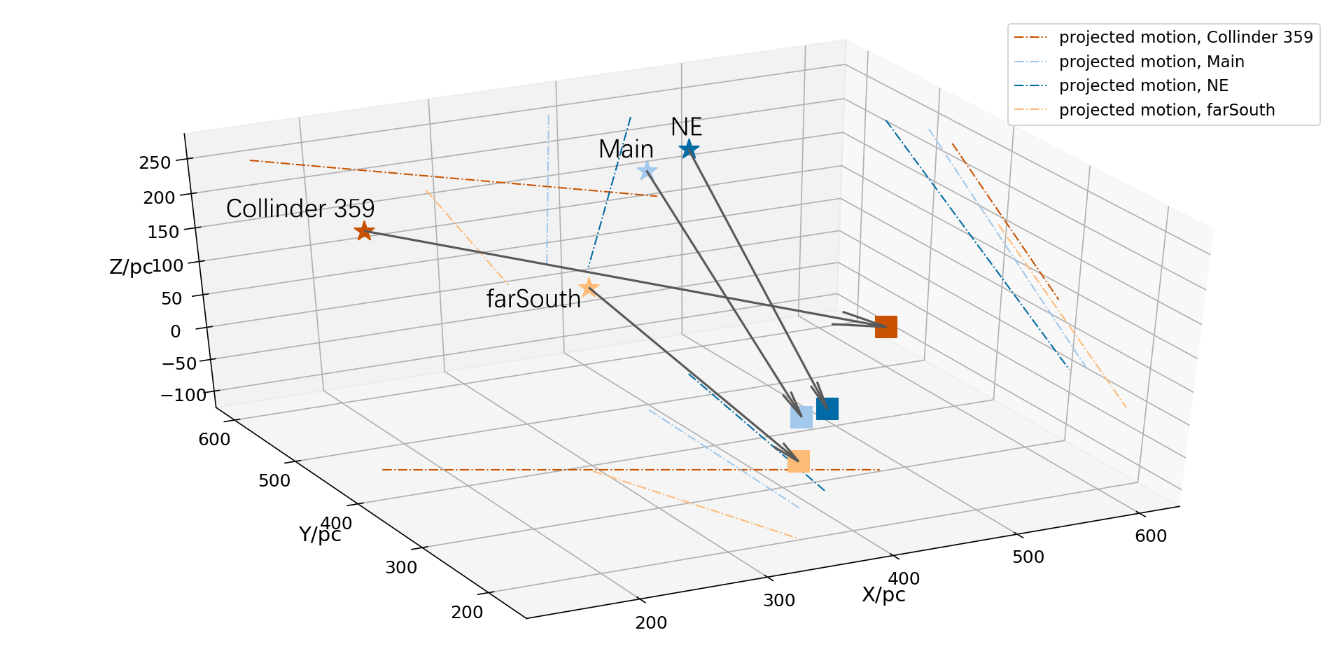
Figure 18: Current position (squares) and inferred position 15 Myr ago (star symbols) (Galactic coordinates, the Sun is at (X,Y,Z) = 0,0,0) of three groups in Serpens and nearby open cluster Collinder 359. Serpens Main is younger than 15 Myr but is still presented. Black arrows represent the space motion of the groups. Colored dashed lines are the projection of space motions into (X,Y), (X,Z) and (Y,Z) planes.

5.3 Co-location of disks and protostars

The disk fraction of a cluster provides an indication of cluster age, relative to the disk fraction in other clusters (e.g. Haisch et al., 2001; Hernández et al., 2008; Bell et al., 2013). In Serpens, some optically bright members are in clusters that have protostars, especially in the active star-forming regions Serpens Main and Serpens NE. Other Serpens members are far from any known protostars but are in groups that still have disks (see Figure 4 of Herczeg et al. 2019).

The overall disk fraction for the optical members of the Serpens star-forming region is 49 of 406 stars (12%), from the sample of high confidence members with reliable photometry (samples without WISE photometry are excluded). This disk fraction suggests ages of 5–10 Myr, roughly consistent with our age estimates.

This disk fraction applies only to the optical members and is not necessarily representative of the entire cluster. An analysis based on the full membership requires significant assumptions and extrapolations. For Serpens Main, the high-confidence members include 17 stars with disks and 62 diskless stars (22% disk fraction, as listed in Table 6). The total statistical population consists of 265 members, as measured from the excess population associated with the cluster (Herczeg et al., 2019). If we assume that the populations are similar, then the optical population would include 72.7 disk stars and 192.3 diskless stars. From infrared surveys, Dunham et al. (2015) identified 222 likely members (excluding AGB stars). Of the stars with Gaia astrometry, 50% of the evolved sources and 86% of the 73 disks are consistent with Serpens membership. In follow-up with the envelope tracer HCO⁺, Heiderman & Evans (2015) confirmed that 88% of candidate protostars in Serpens have an envelope, confirming membership and evolutionary stage. If we assume that all matches are in the statistical population to avoid double-counting, then we find that Serpens Main consists of 45.5 protostars, 122.6 stars with disks, and 197.8 diskless stars. This estimate includes significant uncertainties, including complications from binarity and extrapolations from the well-defined optical sample to the infrared sample, which may be younger. The disk fractions may be underestimated if many diskless sources have high extinctions, either because they have high extinctions or because they are located within or behind the cloud, and were not selected in the Dunham et al. (2015) catalog,

Based on the above arguments, we adopt for Serpens Main a disk fraction of 38% and a disk+protostar fraction of 46%. Similar estimates lead to disk+protostar fractions of 12% for Serpens NE and 16% for Serpens far-South. These disk fractions support our relative ages: Serpens Main is younger than Serpens NE and Serpens far-South. While these disk fractions indicate average ages for the clusters, the presence of protostars, disks, and diskless stars in the same cluster are likely the consequence of an age spread within the cluster (see, e.g. Kristensen & Dunham, 2018).

5.4 Dynamics of the subclusters in and around the Serpens Molecular Cloud

The identification of optically bright members of the Serpens molecular cloud complements previous selections from the infrared. The infrared selections identified several star clusters that are deeply embedded in molecular clouds (e.g., Winston et al., 2009; Kuhn et al., 2013; Dunham et al., 2015). The optically bright members are lightly extincted, some still in clusters and some distributed across the region. The infrared members trace the ongoing star formation, while the optical members trace star formation in the recent past. The ages of these different samples help to quantify when and where the bursts of star formation occurred.

To infer the formation history of Serpens, ages are combined with space velocities of these Serpens groups (Table 8), with proper motions obtained from Herczeg et al. (2019) and the weighted mean radial velocities and associated uncertainty obtained from members with velocities in Gaia DR2. The radial velocities of Serpens Main, NE, farSouth are $-9.6\pm 2.4$ km/s, $-12.1\pm 5.5$ km/s, and $-2.4\pm 2.1$ km/s separately. However, only few stars have radial velocity data (listed in Table 8), and the radial velocity uncertainties are significantly larger than proper motion uncertainties ($\sim 0.2$ mas, corresponding to $0.4$ km/s). Thus, the radial velocities are far less reliable than proper motions, and the radial velocity discrepancy between stars and gas is likely due to the uncertainties of stellar velocity. The radial velocity of Collinder 359 is calculated from Cantat-Gaudin et al. (2018) samples with membership probability $P_{memb}\geq 0.9$ and Gaia radial velocity, leading to $10.8\pm 4.9$ km/s.

With these space motions, the relative locations of the sub-clusters can be traced back in time (Figure 18). The two youngest groups, Serpens Main and Serpens NE (4 Myr and 8.3 Myr), have been co-moving from their birth to present, separated by a distance of $\sim 60$ pc (4 Myr ago) to $\sim 40$ pc now, indicating that they may have similar formation history. The highly embedded regions W40 and Serpens South lack optical members in this study and are expected to be in the same cloud complex as Serpens Main, as suggested by Ortiz-León et al. (2017). The older group, Serpens far-South (17 Myr), has larger velocity difference from Serpens Main (e.g., 4.6 km/s in Galactic X coordinate, 3.2 km/s in Y, and 3.7 km/s in Z). Thus, Serpens far-South may have a different origin from Serpens Main ($\sim 160$ pc away from Serpens Main at the birth of far-South) or had star formation triggered by some interaction that had a different velocity at that location. The open cluster Collinder 359 reached a minimum distance of $\sim 60$ pc to Serpens Main at $\sim 5$ Myr ago, when Serpens Main was born; whether such condition is coincidental or it reflects possible connections between Collinder 359 and Serpens is unclear.

The initial analysis of Gaia DR2 astrometry of the Serpens region by Herczeg et al. (2019) also includes a discussion of ages and kinematic properties of the sub-clusters. In Serpens NE, Herczeg et al. (2019) find that some stars are located outside of the molecular cloud, either because stars were born in a centralized space and were flung away (cluster dynamics) or because feedback from the older stars eroded nearby cloud and changed the birth place of younger stars. If these stars were born at the same spatial location, the velocity dispersion would require that they are $\sim 20$ Myr old. With the age of Serpens NE of 9 Myr, that scenario is more plausible than if the stars were much younger.

In addition to Serpens, some other nearby young star-forming regions also contain several subgroups with different kinematic properties. For example, Krause et al. (2018) studied stars and gas of the Scorpius–Centaurus association and described the following sequential scenario to explain the formation history of the subgroups in this association: the first star-forming activity generated superbubbles, which triggered more star-forming events, with subgroups that move in different directions due to gas interaction. Krause et al. (2018) also suggested that the scenario might apply to many young star-forming regions in the Milky Way. If Serpens has a similar formation scenario, the first star-forming event would start at $\sim 26$ Myr ago (Serpens farS_ext and farSouth), which triggered the second star-forming activity at $\sim 9$ Myr ago (Serpens NE and Main), and the current star-forming events are in W40 (the most embedded region), Serpens Main and NE.

Multiple star-forming events in a single cluster appears to be the common mode of star formation. In a Gaia DR2 study of the Orion OB association , Zari et al. (2019) found in that multiple star-forming events occurred and leaded to the subgroups. In a search for stellar groups in the Taurus field, Liu et al. (2021) identified 8 groups younger than $\sim 4$ Myr and 14 older groups (8-49 Myr). In a smaller region, Esplin & Luhman (2022) found older stars in Corona Australis and inferred a past burst of star formation, likely related to the ongoing star formation in the Coronet Cluster. These processes seem common to nearby low-mass star formation.

6 Conclusions

We develop an SED fitting method for diskless young stellar objects based on empirical color-color relationships from the Pleiades and temperatures measured from APOGEE near-IR spectra by Cottaar et al. (2014). When using stars in Orion to test the method, the fitted temperature is consistent with temperatures from APOGEE spectra (Kounkel et al., 2018) to within $\sim$240 K for diskless stars and $\sim$630 K ($\sim$170 K) for disk stars (with $T_{fit}<$5000 K), all substantial improvements on SED fitting from other commonly used methods. Shortcomings in the method include extinction coefficient variation, dust emission from stellar disk, different surface gravity, and different color-color relations among YSOs.

We collect photometry for high-confidence optical members of the Serpens Molecular Cloud and then fit SEDs with our empirical color-color relationships to estimate temperature and luminosity for each star. The stars belong to several distinct groups in and around the cloud. Subcluster ages range from $\sim 4$ Myr for Serpens Main to $\sim 22$ Myr for dispersed stars located to the south of the cloud for standard non-magnetic evolutionary tracks. The optically bright population is much older than the populations that are revealed from infrared selection criteria, such as the Serpens South region. We then use the ages to discuss possible connections between the distinct subclusters, including a possible explanation similar to the sequential star formation in Sco-Cen OB Association, as inferred by Krause et al. (2018). A deeper understanding of the star formation history of the Serpens Molecular Cloud and any causal connections between different regions will require spectroscopy, especially of infrared-selected members that are not optically visible, and analysis of star and gas motions.

Appendix A Color-color relations

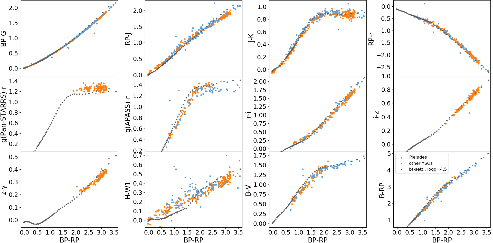
Figure 19: Relations between various colors and $BP-RP$. Red, cyan and blue dots represent colors from Pleiades stars, colors from other YSOs (Pecaut & Mamajek (2013), Gagné et al. (2018), Manara et al. (2013), Manara et al. (2017)), and colors calculated through BT-Settl spectra. A few stars in Pecaut & Mamajek (2013) may contain a dusty disk, according to $H-W1$.

In Section 2, we describe empirical color-color relationships and compare them to models. Here we provide supplemental figures and a Table presenting the colors used in our fits.

Table 9: Color-color table

T/K	BP-RP	J-RP	H-RP	K-RP	W1-RP	W2-RP	g-RP	r-RP	i-RP	z-RP	y-RP	B-RP	V-RP	g’-RP
3000	3.17	-1.93	-2.54	-2.83	-3.02	-3.23	3.51	2.32	0.55	-0.21	-0.61	-	-	-
3100	3.04	-1.86	-2.47	-2.74	-2.92	-3.12	3.38	2.17	0.53	-0.2	-0.56	4.24	2.76	3.39
3200	2.90	-1.79	-2.40	-2.67	-2.83	-3.02	3.25	2.03	0.50	-0.17	-0.52	4.17	2.64	3.33
3300	2.79	-1.73	-2.36	-2.62	-2.76	-2.94	3.15	1.91	0.49	-0.15	-0.48	4.09	2.54	3.26
3400	2.70	-1.69	-2.32	-2.57	-2.71	-2.87	3.05	1.81	0.47	-0.13	-0.44	4.01	2.45	3.19
3500	2.60	-1.64	-2.29	-2.53	-2.66	-2.80	2.96	1.71	0.46	-0.11	-0.40	3.93	2.36	3.12
3600	2.50	-1.59	-2.25	-2.49	-2.61	-2.73	2.86	1.62	0.45	-0.09	-0.37	3.83	2.26	3.03
3700	2.40	-1.54	-2.21	-2.44	-2.55	-2.66	2.76	1.52	0.43	-0.06	-0.33	3.71	2.16	2.93
3800	2.29	-1.49	-2.17	-2.39	-2.49	-2.58	2.65	1.43	0.42	-0.03	-0.28	3.58	2.06	2.82
3900	2.17	-1.43	-2.12	-2.33	-2.42	-2.49	2.53	1.33	0.41	0.00	-0.23	3.44	1.94	2.69
4000	2.05	-1.37	-2.06	-2.25	-2.34	-2.39	2.41	1.23	0.40	0.02	-0.18	3.27	1.82	2.55
4100	1.93	-1.30	-1.98	-2.17	-2.25	-2.28	2.28	1.13	0.39	0.05	-0.14	3.10	1.70	2.41
4200	1.82	-1.24	-1.91	-2.08	-2.16	-2.17	2.15	1.05	0.38	0.09	-0.09	2.93	1.59	2.26
4300	1.72	-1.17	-1.83	-1.99	-2.07	-2.07	2.03	0.97	0.37	0.11	-0.05	2.77	1.49	2.13
4400	1.63	-1.12	-1.75	-1.91	-1.98	-1.97	1.92	0.91	0.36	0.14	-0.01	2.63	1.40	2.00
4500	1.55	-1.06	-1.68	-1.82	-1.89	-1.88	1.81	0.85	0.36	0.16	0.02	2.49	1.31	1.89
4600	1.47	-1.02	-1.60	-1.75	-1.81	-1.79	1.71	0.80	0.35	0.18	0.05	2.37	1.24	1.79
4700	1.40	-0.97	-1.54	-1.67	-1.73	-1.71	1.62	0.76	0.35	0.20	0.07	2.25	1.17	1.70
4800	1.34	-0.93	-1.47	-1.60	-1.66	-1.63	1.54	0.72	0.35	0.22	0.10	2.15	1.11	1.61
4900	1.28	-0.89	-1.41	-1.53	-1.59	-1.56	1.46	0.69	0.34	0.23	0.12	2.05	1.06	1.53
5000	1.23	-0.85	-1.34	-1.46	-1.52	-1.49	1.38	0.66	0.34	0.24	0.14	1.96	1.01	1.45
5200	1.13	-0.78	-1.23	-1.33	-1.39	-1.36	1.23	0.60	0.33	0.26	0.18	1.79	0.91	1.32
5400	1.04	-0.72	-1.12	-1.22	-1.27	-1.24	1.10	0.56	0.33	0.28	0.21	1.63	0.83	1.20
5600	0.95	-0.66	-1.02	-1.11	-1.16	-1.13	0.97	0.52	0.33	0.30	0.24	1.49	0.75	1.09
5800	0.88	-0.60	-0.92	-1.00	-1.05	-1.02	0.84	0.48	0.32	0.31	0.27	1.36	0.68	0.99
6000	0.80	-0.55	-0.83	-0.90	-0.95	-0.92	0.72	0.45	0.32	0.32	0.29	1.24	0.62	0.89
6200	0.74	-0.50	-0.74	-0.81	-0.86	-0.83	-	0.42	0.32	-	-	1.12	0.56	0.81
6400	0.67	-0.46	-0.66	-0.73	-0.77	-0.75	-	0.39	0.31	-	-	1.01	0.51	0.73
6600	0.61	-0.41	-0.59	-0.64	-0.68	-0.66	-	0.37	0.31	-	-	0.91	0.46	0.65
6800	0.55	-0.37	-0.51	-0.57	-0.60	-0.59	-	0.34	0.31	-	-	0.81	0.41	0.58
7000	0.49	-0.33	-0.45	-0.50	-0.53	-0.52	-	0.32	0.30	-	-	0.72	0.36	0.52
7500	0.36	-0.25	-0.31	-0.34	-0.36	-0.36	-	0.28	0.30	-	-	0.52	0.26	0.38
8000	0.24	-0.19	-0.20	-0.23	-0.24	-0.24	-	0.25	0.29	-	-	0.35	0.18	0.26
8500	0.14	-0.13	-0.12	-0.14	-0.14	-0.15	-	0.22	0.29	-	-	0.21	0.12	0.18
9000	0.06	-0.10	-0.07	-0.08	-0.08	-0.09	-	0.21	0.28	-	-	0.10	0.06	0.11
9500	0	-0.07	-0.03	-0.04	-0.03	-0.04	-	-	-	-	-	-	-	-

Appendix B Fitting additional young stars

As mentioned in Section 2.1, some additional young stars are used to expand temperature range of Pan-STARRS photometry. These stars include: a) $<\sim 30$ Myr $\beta$ Pic, $\epsilon$ Cha, $\eta$ Cha, and TW Hya from BANYAN XI and XIII (Gagné et al., 2018; Gagné & Faherty, 2018); b) $\sim 1000$ stars selected from Kounkel & Covey (2019). The Kounkel & Covey (2019) catalog contains $\sim 0.3$ million stars within 1 kpc and with ages from $\sim 1$ Myr to $\sim 10$ Gyr. To select stars younger than or similar to Pleiades, we first pick stars younger than 300 Myr and within 1000 pc from Kounkel & Covey (2019). Then, only stars with photometry of all pass-bands in Section 2 are selected, leaving $\sim 12000$ stars. Finally, since expanding temperature range of Pan-STARRS photometry does not need a large amount of stars (e.g., the Pleiades sample in this method only includes $\sim 300$ stars), we further select $\sim 1000$ stars from the $\sim 12000$ stars, which is done by picking 1000 uniformly distributed numbers between 0 and 3.2 (the $BP-RP$ range of this fitting method), and finding stars with $BP-RP$ locating at these numbers. Such selection assures that the collected stars are basically uniformly distributed in the color range of the fitting, except the bluest end which is too bright for Pan-STARRS photometry.

To investigate whether Pleiades fits the additional young stars well, we use Pleiades to fit these stars, following the method in Section 3. Figure 20 and 21 show the fitted result of BANYAN and Kounkel & Covey (2019) stars. Because there is no APOGEE catalog containing most of these additional stars , the color $BP-RP$ is used for comparison instead of $T_{\rm eff}$.

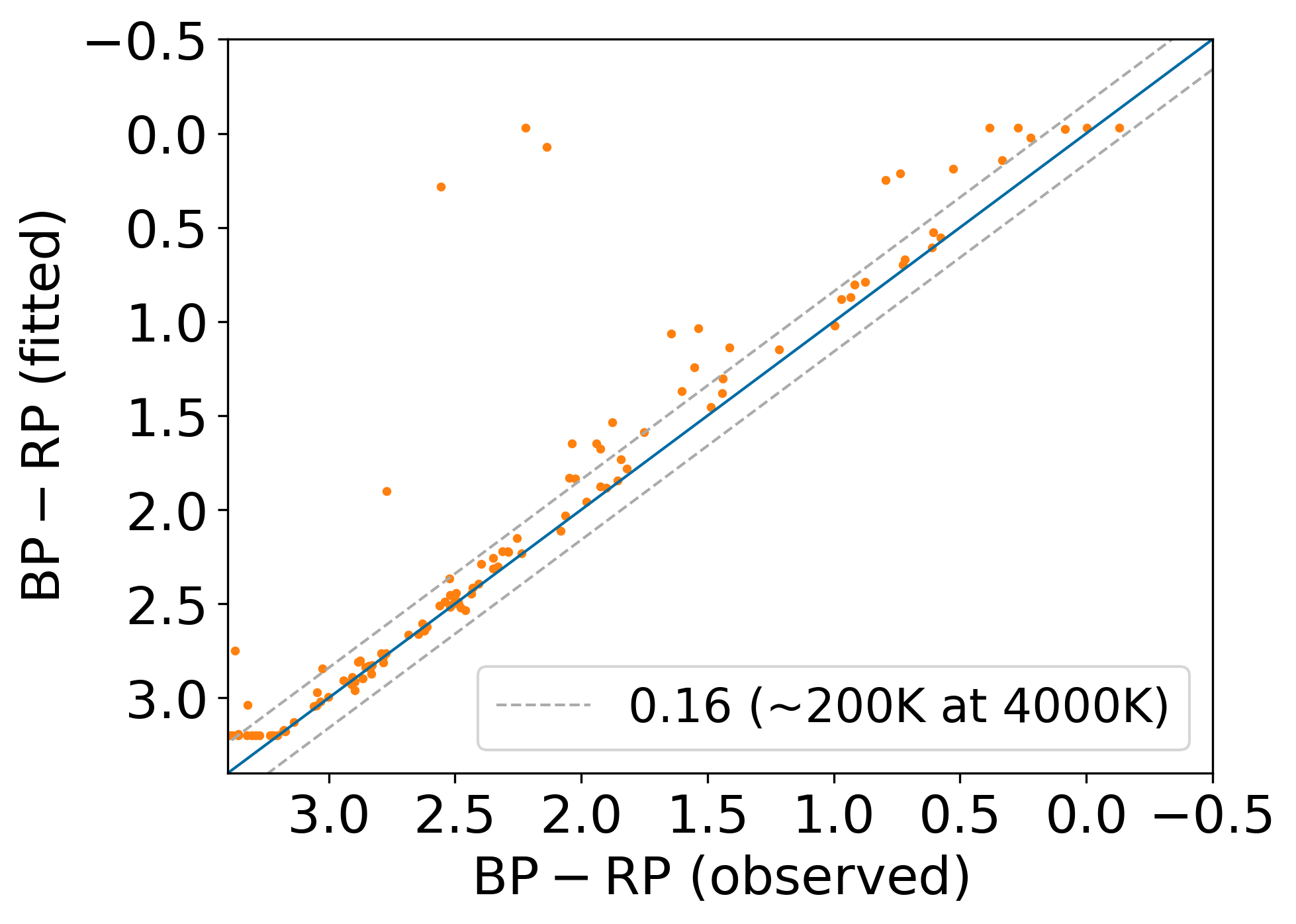
Figure 20: Comparison between observed $BP-RP$ (x-axis) and fitted $BP-RP$ (y-axis) of BANYAN YSOs.

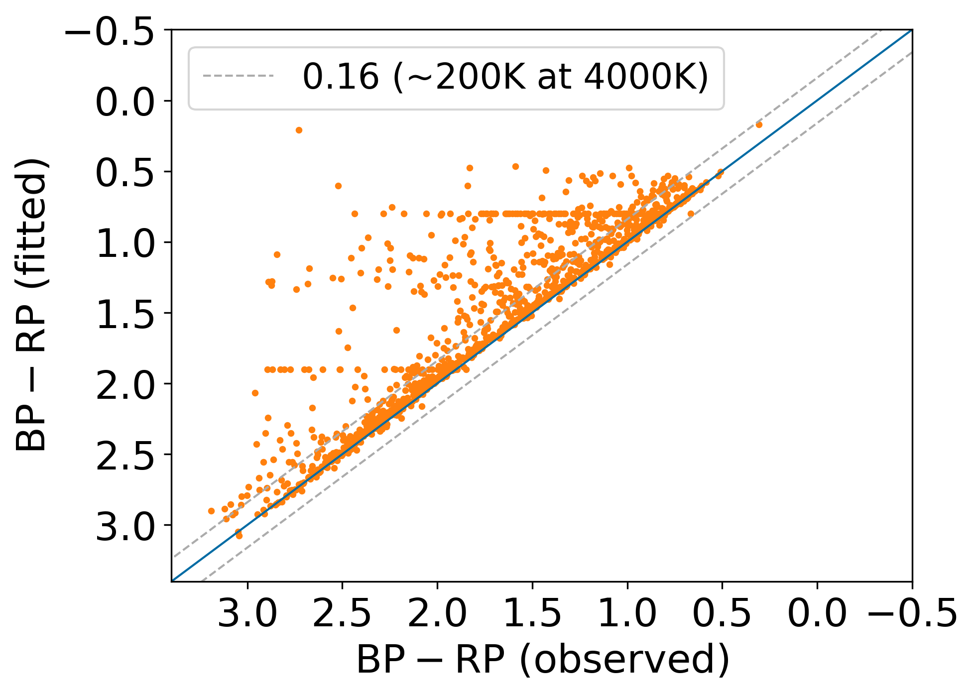
Figure 21: Comparison between observed $BP-RP$ (x-axis) and fitted $BP-RP$ (y-axis) of Kounkel et al. (2019) young stars. Extinction in the fitting is restricted to $A_{V}\geq 0$.

As shown in Figure 20, Pleiades fits well to the cooler YSOs ($BP-RP>2$, corresponding to $\sim 4000$ K). Among the three stars with the bluest fitted $BP-RP$, two have a protoplanetary disk and one has a nearby ($\sim 6$ arcsec) bright source that limits the accuracy of Gaia and 2MASS photometry and may contaminate 2MASS photometry. Pleiades also fits well to the hotter YSOs ($BP-RP<1$, corresponding to $\sim 5500$ K). Three stars at $BP-RP\sim 0.7$ show flux excess in $W1$ and $W2$, thus have bluer fitted $BP-RP$. Their fitted $BP-RP$ is close to observed values after removing WISE data. Stars at $1<BP-RP<2$ tend to have bluer fitted $BP-RP$, which is likely due to surface gravity difference.

Figure 21 also shows a good consistency between fitted $BP-RP$ and observed $BP-RP$. Some stars may have obvious extinction and/or disk, thus have bluer fitted $BP-RP$. The line structure at $(BP-RP)_{\rm fit}\sim 1.9$ and $(BP-RP)_{\rm fit}\sim 0.8$ corresponds to $BP-RP$ range of Pleiades Pan-STARRS and APASS data. The fitted $BP-RP$ is hardly redder than the observed $BP-RP$, due to the $A_{V}$ constraint ($>=0$) in the fitting. We then select additional young stars based on the result above, as described in Section 2.1.

Appendix C Age estimate for Collinder 359

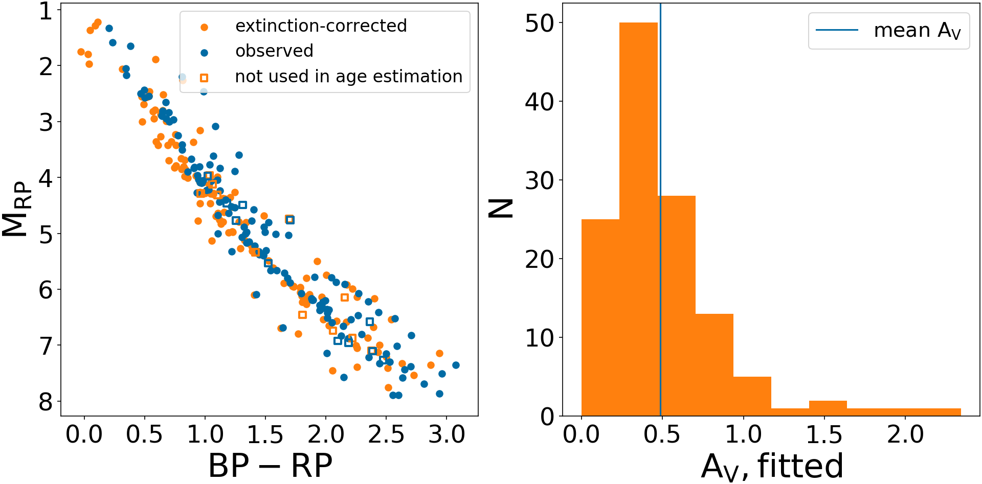
Figure 22: Gaia EDR3 color-magnitude diagram (left panel) and distribution of best-fit $A_{V}$ (right panel) of Collinder 359. The color-magnitude diagram includes the observed (blue) and extinction-corrected (orange) colors and magnitudes. Unfilled symbols are stars which are not used in calculating ages, and these stars are not included in the right panel.

Collinder 359 is a young open cluster located $\sim 130$ pc away from Serpens Main. The distance to Collinder 359 is $\sim 560$ pc (Cantat-Gaudin et al., 2018). In Section 5.4, we evaluate the possible connection between Collinder 359 and the ongoing star formation in Serpens, since they are physically located 130 pc away from each other. Collinder 359 has been previously estimated to have an age of $\sim 60$ Myr (Lodieu et al., 2006) and $\sim 28$ Myr (Kharchenko et al., 2013).

We re-evaluate the age of Collinder 359 as 21 Myr from the Feiden (2016) non-magnetic tracks, in a method consistent with the approach applied to the Serpens sample of young stars. The age is estimated from 127 stars selected from 138 members in Cantat-Gaudin et al. (2018) with membership probability $P_{\rm memb}\geq 0.9$, with 11 stars excluded due to their visual binaries that are unresolved by 2MASS. Figure 22 shows color-magnitude diagram and $A_{V}$ distribution of these Collinder 359 stars. After fitting a three-degree polynomial to the color-magnitude diagram, the rms is 0.41 for the observed CMD, 0.40 for the extinction-corrected CMD based on SED fitting result, and 0.38 for the observed CMD when using a single distance for all stars. The SED fitting result does not significantly affect the rms in color-magnitude diagram, due to the tight $A_{V}$ distribution of Collinder 359. The average fitted $A_{V}\sim$ 0.5 mag is consistent with $A_{V}\sim 0.5$ mag estimated by Kharchenko et al. (2013).

References

- Allard et al. (2012) Allard, F., Homeier, D., & Freytag, B. 2012, Philosophical Transactions of the Royal Society of London Series A, 370, 2765, doi: 10.1098/rsta.2011.0269
- Asplund et al. (2009) Asplund, M., Grevesse, N., Sauval, A. J., & Scott, P. 2009, ARA&A, 47, 481, doi: 10.1146/annurev.astro.46.060407.145222
- Astropy Collaboration et al. (2013) Astropy Collaboration, Robitaille, T. P., Tollerud, E. J., et al. 2013, A&A, 558, A33, doi: 10.1051/0004-6361/201322068
- Barrado et al. (2016) Barrado, D., Bouy, H., Bouvier, J., et al. 2016, A&A, 596, A113, doi: 10.1051/0004-6361/201629103
- Basri et al. (1996) Basri, G., Marcy, G. W., & Graham, J. R. 1996, ApJ, 458, 600, doi: 10.1086/176842
- Bayo et al. (2008) Bayo, A., Rodrigo, C., Barrado Y Navascués, D., et al. 2008, A&A, 492, 277, doi: 10.1051/0004-6361:200810395
- Bell et al. (2012) Bell, C. P. M., Naylor, T., Mayne, N. J., Jeffries, R. D., & Littlefair, S. P. 2012, MNRAS, 424, 3178, doi: 10.1111/j.1365-2966.2012.21496.x
- Bell et al. (2013) —. 2013, MNRAS, 434, 806, doi: 10.1093/mnras/stt1075
- Binks & Jeffries (2014) Binks, A. S., & Jeffries, R. D. 2014, MNRAS, 438, L11, doi: 10.1093/mnrasl/slt141
- Bouvier et al. (2018) Bouvier, J., Barrado, D., Moraux, E., et al. 2018, A&A, 613, A63, doi: 10.1051/0004-6361/201731881
- Bouy et al. (2015) Bouy, H., Bertin, E., Sarro, L. M., et al. 2015, A&A, 577, A148, doi: 10.1051/0004-6361/201425019
- Bressan et al. (2012) Bressan, A., Marigo, P., Girardi, L., et al. 2012, MNRAS, 427, 127, doi: 10.1111/j.1365-2966.2012.21948.x
- Brott & Hauschildt (2005) Brott, I., & Hauschildt, P. H. 2005, in ESA Special Publication, Vol. 576, The Three-Dimensional Universe with Gaia, ed. C. Turon, K. S. O’Flaherty, & M. A. C. Perryman, 565. https://arxiv.org/abs/astro-ph/0503395
- Cantat-Gaudin et al. (2018) Cantat-Gaudin, T., Jordi, C., Vallenari, A., et al. 2018, A&A, 618, A93, doi: 10.1051/0004-6361/201833476
- Carrera et al. (2019) Carrera, R., Bragaglia, A., Cantat-Gaudin, T., et al. 2019, A&A, 623, A80, doi: 10.1051/0004-6361/201834546
- Castelli & Kurucz (2003) Castelli, F., & Kurucz, R. L. 2003, in Modelling of Stellar Atmospheres, ed. N. Piskunov, W. W. Weiss, & D. F. Gray, Vol. 210, A20. https://arxiv.org/abs/astro-ph/0405087
- Chambers et al. (2016) Chambers, K. C., Magnier, E. A., Metcalfe, N., et al. 2016, arXiv e-prints, arXiv:1612.05560. https://arxiv.org/abs/1612.05560
- Chen et al. (2015) Chen, Y., Bressan, A., Girardi, L., et al. 2015, MNRAS, 452, 1068, doi: 10.1093/mnras/stv1281
- Chen et al. (2014) Chen, Y., Girardi, L., Bressan, A., et al. 2014, MNRAS, 444, 2525, doi: 10.1093/mnras/stu1605
- Cottaar et al. (2014) Cottaar, M., Covey, K. R., Meyer, M. R., et al. 2014, ApJ, 794, 125, doi: 10.1088/0004-637X/794/2/125
- Cutri et al. (2003) Cutri, R. M., Skrutskie, M. F., van Dyk, S., et al. 2003, VizieR Online Data Catalog, II/246
- Cutri et al. (2021) Cutri, R. M., Wright, E. L., Conrow, T., et al. 2021, VizieR Online Data Catalog, II/328
- Da Rio et al. (2016) Da Rio, N., Tan, J. C., Covey, K. R., et al. 2016, ApJ, 818, 59, doi: 10.3847/0004-637X/818/1/59
- Davies (2020) Davies, C. L. 2020, arXiv e-prints, arXiv:2008.07800. https://arxiv.org/abs/2008.07800
- Dunham et al. (2015) Dunham, M. M., Allen, L. E., Evans, Neal J., I., et al. 2015, ApJS, 220, 11, doi: 10.1088/0067-0049/220/1/11
- Eiroa et al. (2008) Eiroa, C., Djupvik, A. A., & Casali, M. M. 2008, The Serpens Molecular Cloud, ed. B. Reipurth, Vol. 5, 693
- Erickson et al. (2015) Erickson, K. L., Wilking, B. A., Meyer, M. R., et al. 2015, AJ, 149, 103, doi: 10.1088/0004-6256/149/3/103
- Esplin & Luhman (2022) Esplin, T. L., & Luhman, K. L. 2022, AJ, 163, 64, doi: 10.3847/1538-3881/ac3e64
- Evans et al. (2003) Evans, Neal J., I., Allen, L. E., Blake, G. A., et al. 2003, PASP, 115, 965, doi: 10.1086/376697
- Fang et al. (2013) Fang, M., Kim, J. S., van Boekel, R., et al. 2013, ApJS, 207, 5, doi: 10.1088/0067-0049/207/1/5
- Fang et al. (2017) Fang, M., Kim, J. S., Pascucci, I., et al. 2017, AJ, 153, 188, doi: 10.3847/1538-3881/aa647b
- Fang et al. (2016) Fang, X.-S., Zhao, G., Zhao, J.-K., Chen, Y.-Q., & Bharat Kumar, Y. 2016, MNRAS, 463, 2494, doi: 10.1093/mnras/stw1923
- Feiden (2016) Feiden, G. A. 2016, A&A, 593, A99, doi: 10.1051/0004-6361/201527613
- Fischer et al. (2011) Fischer, W., Edwards, S., Hillenbrand, L., & Kwan, J. 2011, ApJ, 730, 73, doi: 10.1088/0004-637X/730/2/73
- Fitzpatrick (1999) Fitzpatrick, E. L. 1999, PASP, 111, 63, doi: 10.1086/316293
- Forbrich et al. (2010) Forbrich, J., Tappe, A., Robitaille, T., et al. 2010, ApJ, 716, 1453, doi: 10.1088/0004-637X/716/2/1453
- Gagné et al. (2020) Gagné, J., David, T. J., Mamajek, E. E., et al. 2020, ApJ, 903, 96, doi: 10.3847/1538-4357/abb77e
- Gagné & Faherty (2018) Gagné, J., & Faherty, J. K. 2018, ApJ, 862, 138, doi: 10.3847/1538-4357/aaca2e
- Gagné et al. (2018) Gagné, J., Mamajek, E. E., Malo, L., et al. 2018, ApJ, 856, 23, doi: 10.3847/1538-4357/aaae09
- Gahm et al. (2008) Gahm, G. F., Walter, F. M., Stempels, H. C., Petrov, P. P., & Herczeg, G. J. 2008, A&A, 482, L35, doi: 10.1051/0004-6361:200809488
- Gaia Collaboration et al. (2018) Gaia Collaboration, Babusiaux, C., van Leeuwen, F., et al. 2018, A&A, 616, A10, doi: 10.1051/0004-6361/201832843
- Gaia Collaboration et al. (2021) Gaia Collaboration, Brown, A. G. A., Vallenari, A., et al. 2021, A&A, 649, A1, doi: 10.1051/0004-6361/202039657
- Getman et al. (2017) Getman, K. V., Broos, P. S., Kuhn, M. A., et al. 2017, ApJS, 229, 28, doi: 10.3847/1538-4365/229/2/28
- Getman et al. (2014a) Getman, K. V., Feigelson, E. D., & Kuhn, M. A. 2014a, ApJ, 787, 109, doi: 10.1088/0004-637X/787/2/109
- Getman et al. (2014b) Getman, K. V., Feigelson, E. D., Kuhn, M. A., et al. 2014b, ApJ, 787, 108, doi: 10.1088/0004-637X/787/2/108
- Grankin et al. (2008) Grankin, K. N., Bouvier, J., Herbst, W., & Melnikov, S. Y. 2008, A&A, 479, 827, doi: 10.1051/0004-6361:20078476
- Grankin et al. (2007) Grankin, K. N., Melnikov, S. Y., Bouvier, J., Herbst, W., & Shevchenko, V. S. 2007, A&A, 461, 183, doi: 10.1051/0004-6361:20065489
- Gully-Santiago et al. (2017) Gully-Santiago, M. A., Herczeg, G. J., Czekala, I., et al. 2017, ApJ, 836, 200, doi: 10.3847/1538-4357/836/2/200
- Guo et al. (2018a) Guo, Z., Gully-Santiago, M., & Herczeg, G. J. 2018a, ApJ, 868, 143, doi: 10.3847/1538-4357/aaeb9b
- Guo et al. (2018b) Guo, Z., Herczeg, G. J., Jose, J., et al. 2018b, ApJ, 852, 56, doi: 10.3847/1538-4357/aa9e52
- Gutermuth et al. (2008) Gutermuth, R. A., Bourke, T. L., Allen, L. E., et al. 2008, ApJ, 673, L151, doi: 10.1086/528710
- Haisch et al. (2001) Haisch, Karl E., J., Lada, E. A., & Lada, C. J. 2001, ApJ, 553, L153, doi: 10.1086/320685
- Hartmann et al. (2016) Hartmann, L., Herczeg, G., & Calvet, N. 2016, ARA&A, 54, 135, doi: 10.1146/annurev-astro-081915-023347
- Heiderman & Evans (2015) Heiderman, A., & Evans, Neal J., I. 2015, ApJ, 806, 231, doi: 10.1088/0004-637X/806/2/231
- Henden et al. (2015) Henden, A. A., Levine, S., Terrell, D., & Welch, D. L. 2015, in American Astronomical Society Meeting Abstracts, Vol. 225, American Astronomical Society Meeting Abstracts #225, 336.16
- Herczeg & Hillenbrand (2015) Herczeg, G. J., & Hillenbrand, L. A. 2015, ApJ, 808, 23, doi: 10.1088/0004-637X/808/1/23
- Herczeg et al. (2019) Herczeg, G. J., Kuhn, M. A., Zhou, X., et al. 2019, ApJ, 878, 111, doi: 10.3847/1538-4357/ab1d67
- Hernández et al. (2008) Hernández, J., Hartmann, L., Calvet, N., et al. 2008, ApJ, 686, 1195, doi: 10.1086/591224
- Hernández et al. (2010) Hernández, J., Morales-Calderon, M., Calvet, N., et al. 2010, ApJ, 722, 1226, doi: 10.1088/0004-637X/722/2/1226
- Hernández et al. (2007) Hernández, J., Hartmann, L., Megeath, T., et al. 2007, ApJ, 662, 1067, doi: 10.1086/513735
- Husser et al. (2013) Husser, T. O., Wende-von Berg, S., Dreizler, S., et al. 2013, A&A, 553, A6, doi: 10.1051/0004-6361/201219058
- Indebetouw et al. (2005) Indebetouw, R., Mathis, J. S., Babler, B. L., et al. 2005, ApJ, 619, 931, doi: 10.1086/426679
- Kado-Fong et al. (2016) Kado-Fong, E., Williams, P. K. G., Mann, A. W., et al. 2016, ApJ, 833, 281, doi: 10.3847/1538-4357/833/2/281
- Kharchenko et al. (2013) Kharchenko, N. V., Piskunov, A. E., Schilbach, E., Röser, S., & Scholz, R. D. 2013, A&A, 558, A53, doi: 10.1051/0004-6361/201322302
- Kochanek et al. (2017) Kochanek, C. S., Shappee, B. J., Stanek, K. Z., et al. 2017, PASP, 129, 104502, doi: 10.1088/1538-3873/aa80d9
- Könyves et al. (2015) Könyves, V., André, P., Men’shchikov, A., et al. 2015, A&A, 584, A91, doi: 10.1051/0004-6361/201525861
- Kounkel & Covey (2019) Kounkel, M., & Covey, K. 2019, AJ, 158, 122, doi: 10.3847/1538-3881/ab339a
- Kounkel et al. (2018) Kounkel, M., Covey, K., Suárez, G., et al. 2018, AJ, 156, 84, doi: 10.3847/1538-3881/aad1f1
- Kounkel et al. (2019) Kounkel, M., Covey, K., Moe, M., et al. 2019, AJ, 157, 196, doi: 10.3847/1538-3881/ab13b1
- Krause et al. (2018) Krause, M. G. H., Burkert, A., Diehl, R., et al. 2018, A&A, 619, A120, doi: 10.1051/0004-6361/201732416
- Kristensen & Dunham (2018) Kristensen, L. E., & Dunham, M. M. 2018, A&A, 618, A158, doi: 10.1051/0004-6361/201731584
- Kuhn et al. (2010) Kuhn, M. A., Getman, K. V., Feigelson, E. D., et al. 2010, ApJ, 725, 2485, doi: 10.1088/0004-637X/725/2/2485
- Kuhn et al. (2013) Kuhn, M. A., Povich, M. S., Luhman, K. L., et al. 2013, ApJS, 209, 29, doi: 10.1088/0067-0049/209/2/29
- Lançon et al. (2020) Lançon, A., Gonneau, A., Verro, K., et al. 2020, arXiv e-prints, arXiv:2012.09129. https://arxiv.org/abs/2012.09129
- Lee et al. (2021) Lee, J.-E., Lee, S., Lee, S., et al. 2021, arXiv e-prints, arXiv:2106.11518. https://arxiv.org/abs/2106.11518
- Liu et al. (2021) Liu, J., Fang, M., Tian, H., et al. 2021, ApJS, 254, 20, doi: 10.3847/1538-4365/abf4d1
- Lodieu et al. (2006) Lodieu, N., Bouvier, J., James, D. J., et al. 2006, A&A, 450, 147, doi: 10.1051/0004-6361:20054105
- Luhman & Esplin (2020) Luhman, K. L., & Esplin, T. L. 2020, AJ, 160, 44, doi: 10.3847/1538-3881/ab9599
- Mallick et al. (2013) Mallick, K. K., Kumar, M. S. N., Ojha, D. K., et al. 2013, ApJ, 779, 113, doi: 10.1088/0004-637X/779/2/113
- Manara et al. (2017) Manara, C. F., Frasca, A., Alcalá, J. M., et al. 2017, A&A, 605, A86, doi: 10.1051/0004-6361/201730807
- Manara et al. (2013) Manara, C. F., Testi, L., Rigliaco, E., et al. 2013, A&A, 551, A107, doi: 10.1051/0004-6361/201220921
- Mann et al. (2015) Mann, A. W., Feiden, G. A., Gaidos, E., Boyajian, T., & von Braun, K. 2015, ApJ, 804, 64, doi: 10.1088/0004-637X/804/1/64
- Mayne et al. (2007) Mayne, N. J., Naylor, T., Littlefair, S. P., Saunders, E. S., & Jeffries, R. D. 2007, MNRAS, 375, 1220, doi: 10.1111/j.1365-2966.2006.11347.x
- Megeath et al. (2012) Megeath, S. T., Gutermuth, R., Muzerolle, J., et al. 2012, AJ, 144, 192, doi: 10.1088/0004-6256/144/6/192
- Oliveira et al. (2013) Oliveira, I., Merín, B., Pontoppidan, K. M., & van Dishoeck, E. F. 2013, ApJ, 762, 128, doi: 10.1088/0004-637X/762/2/128
- Ortiz-León et al. (2017) Ortiz-León, G. N., Dzib, S. A., Kounkel, M. A., et al. 2017, ApJ, 834, 143, doi: 10.3847/1538-4357/834/2/143
- Pecaut & Mamajek (2013) Pecaut, M. J., & Mamajek, E. E. 2013, ApJS, 208, 9, doi: 10.1088/0067-0049/208/1/9
- Povich et al. (2013) Povich, M. S., Kuhn, M. A., Getman, K. V., et al. 2013, ApJS, 209, 31, doi: 10.1088/0067-0049/209/2/31
- Prato et al. (2008) Prato, L., Rice, E. L., & Dame, T. M. 2008, Where are all the Young Stars in Aquila?, ed. B. Reipurth, Vol. 4, 18
- Prisinzano et al. (2008) Prisinzano, L., Micela, G., Flaccomio, E., et al. 2008, ApJ, 677, 401, doi: 10.1086/528842
- Robitaille (2017) Robitaille, T. P. 2017, A&A, 600, A11, doi: 10.1051/0004-6361/201425486
- Robitaille et al. (2007) Robitaille, T. P., Whitney, B. A., Indebetouw, R., & Wood, K. 2007, ApJS, 169, 328, doi: 10.1086/512039
- Rodney & Reipurth (2008) Rodney, S. A., & Reipurth, B. 2008, The W40 Cloud Complex, ed. B. Reipurth, Vol. 5, 683
- Rodrigo & Solano (2020) Rodrigo, C., & Solano, E. 2020, in XIV.0 Scientific Meeting (virtual) of the Spanish Astronomical Society, 182
- Rodrigo et al. (2012) Rodrigo, C., Solano, E., & Bayo, A. 2012, SVO Filter Profile Service Version 1.0, IVOA Working Draft 15 October 2012, doi: 10.5479/ADS/bib/2012ivoa.rept.1015R
- Rumble et al. (2015) Rumble, D., Hatchell, J., Gutermuth, R. A., et al. 2015, MNRAS, 448, 1551, doi: 10.1093/mnras/stu2695
- Shappee et al. (2014) Shappee, B. J., Prieto, J. L., Grupe, D., et al. 2014, ApJ, 788, 48, doi: 10.1088/0004-637X/788/1/48
- Sicilia-Aguilar et al. (2004) Sicilia-Aguilar, A., Hartmann, L. W., Briceño, C., Muzerolle, J., & Calvet, N. 2004, AJ, 128, 805, doi: 10.1086/422432
- Skrutskie et al. (2019) Skrutskie, M. F., Cutri, R. M., Stiening, R., et al. 2019, 2MASS All-Sky Point Source Catalog, IPAC, doi: 10.26131/IRSA2
- Soderblom et al. (2014) Soderblom, D. R., Hillenbrand, L. A., Jeffries, R. D., Mamajek, E. E., & Naylor, T. 2014, in Protostars and Planets VI, ed. H. Beuther, R. S. Klessen, C. P. Dullemond, & T. Henning, 219, doi: 10.2458/azu_uapress_9780816531240-ch010
- Soderblom et al. (2009) Soderblom, D. R., Laskar, T., Valenti, J. A., Stauffer, J. R., & Rebull, L. M. 2009, AJ, 138, 1292, doi: 10.1088/0004-6256/138/5/1292
- Somers et al. (2020) Somers, G., Cao, L., & Pinsonneault, M. H. 2020, ApJ, 891, 29, doi: 10.3847/1538-4357/ab722e
- Somers & Stassun (2017) Somers, G., & Stassun, K. G. 2017, AJ, 153, 101, doi: 10.3847/1538-3881/153/3/101
- Soubiran et al. (2018) Soubiran, C., Cantat-Gaudin, T., Romero-Gómez, M., et al. 2018, A&A, 619, A155, doi: 10.1051/0004-6361/201834020
- Spina et al. (2017) Spina, L., Randich, S., Magrini, L., et al. 2017, A&A, 601, A70, doi: 10.1051/0004-6361/201630078
- Stauffer et al. (2003) Stauffer, J. R., Jones, B. F., Backman, D., et al. 2003, AJ, 126, 833, doi: 10.1086/376739
- Stauffer et al. (1998) Stauffer, J. R., Schild, R., Barrado y Navascués, D., et al. 1998, ApJ, 504, 805, doi: 10.1086/306095
- Su et al. (2020) Su, Y., Yang, J., Yan, Q.-Z., et al. 2020, ApJ, 893, 91, doi: 10.3847/1538-4357/ab7fff
- Suárez et al. (2017) Suárez, G., Downes, J. J., Román-Zúñiga, C., et al. 2017, AJ, 154, 14, doi: 10.3847/1538-3881/aa733a
- Tang et al. (2014) Tang, J., Bressan, A., Rosenfield, P., et al. 2014, MNRAS, 445, 4287, doi: 10.1093/mnras/stu2029
- Tonry et al. (2012) Tonry, J. L., Stubbs, C. W., Lykke, K. R., et al. 2012, ApJ, 750, 99, doi: 10.1088/0004-637X/750/2/99
- Vázquez-Semadeni et al. (2018) Vázquez-Semadeni, E., Zamora-Avilés, M., Galván-Madrid, R., & Forbrich, J. 2018, MNRAS, 479, 3254, doi: 10.1093/mnras/sty1586
- Venuti et al. (2021) Venuti, L., Cody, A. M., Rebull, L. M., et al. 2021, AJ, 162, 101, doi: 10.3847/1538-3881/ac0536
- Virtanen et al. (2019) Virtanen, P., Gommers, R., Oliphant, T. E., et al. 2019, arXiv e-prints, arXiv:1907.10121. https://arxiv.org/abs/1907.10121
- Wang & Chen (2019) Wang, S., & Chen, X. 2019, ApJ, 877, 116, doi: 10.3847/1538-4357/ab1c61
- Williams & Cieza (2011) Williams, J. P., & Cieza, L. A. 2011, ARA&A, 49, 67, doi: 10.1146/annurev-astro-081710-102548
- Winston et al. (2009) Winston, E., Megeath, S. T., Wolk, S. J., et al. 2009, AJ, 137, 4777, doi: 10.1088/0004-6256/137/6/4777
- Wright et al. (2019) Wright, E. L., Eisenhardt, P. R. M., Mainzer, A. K., et al. 2019, AllWISE Source Catalog, IPAC, doi: 10.26131/IRSA1
- Zari et al. (2019) Zari, E., Brown, A. G. A., & de Zeeuw, P. T. 2019, A&A, 628, A123, doi: 10.1051/0004-6361/201935781