RCP: Recurrent Closest Point for Scene Flow Estimation on 3D Point Clouds

Abstract

3D motion estimation including scene flow and point cloud registration has drawn increasing interest. Inspired by 2D flow estimation, recent methods employ deep neural networks to construct the cost volume for estimating accurate 3D flow. However, these methods are limited by the fact that it is difficult to define a search window on point clouds because of the irregular data structure. In this paper, we avoid this irregularity by a simple yet effective method. We decompose the problem into two interlaced stages, where the 3D flows are optimized point-wisely at the first stage and then globally regularized in a recurrent network at the second stage. Therefore, the recurrent network only receives the regular point-wise information as the input. In the experiments, we evaluate the proposed method on both the 3D scene flow estimation and the point cloud registration task. For 3D scene flow estimation, we make comparisons on the widely used FlyingThings3D [32] and KITTI [33] datasets. For point cloud registration, we follow previous works and evaluate the data pairs with large pose and partially overlapping from ModelNet40 [65]. The results show that our method outperforms the previous method and achieves a new state-of-the-art performance on both 3D scene flow estimation and point cloud registration, which demonstrates the superiority of the proposed zero-order method on irregular point cloud data. Our source code is available at https://github.com/gxd1994/RCP.

iter=0

iter=3

iter=7

iter=14

Figure 1: Visualization of the results on the KITTI scene flow dataset. With the increasing number of alternate optimizations, the source point cloud (in green) is gradually aligned with the target point cloud (in blue).

1 Introduction

Motion estimation is a fundamental building block for numerous applications such as robotics, augmented reality and autonomous driving. The low-level motion cues can serve other higher-level tasks such as object detection and action recognition. Given a pair or a sequence of images, we can estimate 2D flow fields from optical flow estimation by either classic variational methods or modern deep learning methods [25, 51, 52].

Different from the scene flow methods that extend 2D optical flow to stereoscopic or RGB-D image sequences [24, 21], increasing attention has been paid to the direct 3D flow estimation on point clouds recently, which has several advantages over image based methods for a variety of applications. For example, one of the most prominent benefits is that it avoids the image sensor readings and the additional computation of depth from images for autonomous driving, which enables low-latency 3D flow estimation for a high-speed driving vehicle. While for augmented reality, especially for AR glasses, the 3D flow estimation on point clouds enables the computation distribution on the cloud server because it saves much more transmission bandwidth than images. It also protects the privacy of the surrounding people by not using images.

Therefore, some learning based methods [61, 30, 18, 2, 27] utilizes the recent advances made for high-level tasks and customize the scene flow estimation specifically for point clouds. These methods predict the 3D flow vectors from cost-volumes, where similarity costs between 3D points from two point cloud sets are measured. However, different from the cost-volumes in 2D optical flow that search a fixed regular neighborhood around a pixel in consecutive images [25, 51, 52], it is impossible to define such a search window on point clouds because of the irregular data structure. Therefore, previous works like  [30, 64, 27, 18], they designed some complicated layers to measure the point-to-patch cost or patch-to-patch cost.

In this paper, we avoid this irregularity by a simple and effective method. We decompose the problem into two interlaced stages, where the 3D flows are optimized point-wisely at the first stage and then globally regularized in a recurrent network at the second stage. Therefore, the recurrent network only receives the regular point-wise information as the input. Besides the scene flow estimation, our method also enables another important motion estimation task that registers two point clouds with the different 6-DOF pose. Since we only measure the point-to-point costs, we avoid the discretization of the 6DOF solution space, which is difficult because the rotation vector and the translation vector are two different variables that have different scales and ranges.

To evaluate the proposed method, we conduct experiments on both the 3D scene flow estimation and the point cloud registration. For 3D scene flow estimation, we made comparisons on the widely used FlyingThings3D [32] and KITTI [33] benchmark. For point cloud registration, we follow the previous works and generate data pairs with large pose and partially overlapping from ModelNet40 [65]. We have achieved state-of-the-art results on both 3D scene flow estimation and point cloud registration, which demonstrate the superiority of the proposed zero-order method on irregular point cloud data.

2 Related work

Point Cloud Networks.

Prior to the emergency of neural networks, various hand-crafted 3D feature descriptors have been proposed based on the heuristic knowledge [20]. These descriptors usually accumulate measurements to histograms based on the spatial coordinates [14, 26, 54] or the geometry attributes [6, 44]. Other works such as PFH [43] and FPFH [42] have been proposed the descriptors which are rotation-invariant. Traditional features, however, are designed by hand and cannot be too complicated. More recently, more methods have begun to employ the deep neural networks to learn the features. 3DMatch [70] utilizes a contrastive loss to train a descriptor with 3D convolutional neural networks, but the voxelization leads to a loss of feature quality. To solve this, PPFNet [10] uses the PointNet [38] to directly learn the point cloud features. Also, the salient keypoints are detected to describe the point clouds [28, 68]. In this work, we use PointNet++ [39] to extract the point cloud features considering its strong feature representation ability.

3D Flow Estimation on Point Clouds.

The task of scene flow estimation is first introduced in [59] and then developed from images [24, 21] to point clouds [11, 57, 56]. [11] formulates the scene flow estimation problem as an energy minimization problem. [57] constructs occupancy grids and filters the background before the energy minimization and then refine the results with filtering after. An encoding network is introduced in a following up work to learn features from the occupancy grid [56].

Recently, more methods use deep neural networks for 3D flow estimation [61, 30, 18, 2, 27, 64]. A network that learns hierarchical features of point clouds and flow embeddings representing point motions is designed in FlowNet3D [30]. A bilateral convolutional layer which projects the point cloud to the permutohedral lattice is proposed in HPLFlowNet [18]. PointPWC-Net [64] proposes a learnable cost volume layer along with upsample and warping layers to build a coarse-to-fine deep network to efficiently handle point cloud. FLOT [37] uses optimal transport tools to estimate the scene flow without using multiscale analysis. Recent works [52, 29, 34, 19] get promising results by using the model unrolling method, FlowStep3D [27] adopts GRU[7] to iteratively refine the scene flow and show excellent results. However, all the above methods need to define the cost volume, which is difficult to design considering the irregularity of the point clouds. In contrast, we avoid this irregularity by optimizing the cost point-wisely and sending the regular point-wise information to a recurrent network.

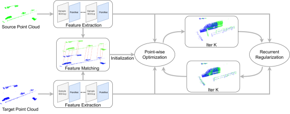
Figure 2: Overview of our framework. We first extract the point cloud features by a shared PointNet++ [39] backbone, followed by the sinkhorn algorithm [48] to get the initialized results from feature matching. Then, we decompose the problem into two sub-problems and utilize the proposed point-wise optimization and recurrent regularization modules to estimate either the 3D scene flow or the transformation.

Point Cloud Registration.

The task of point cloud registration is to find the spatial transformation between two point clouds. Traditional methods are mainly based on the iterative closest point (ICP)[3, 47] and its variants[48, 55, 67, 16, 40, 36, 41]. Recent works learn deep neural networks for point cloud registration and can be divided into two streams. One stream[71, 8, 17, 12, 35, 1, 23] studies how to leverage better point cloud feature presentation in off-the-shelf optimization. PointNetLK[1] defines a feature-metric distance between point clouds, which is measured by the features from PointNet[38], and unrolls the classical Lucas & Kanade (LK) algorithm into a recurrent network to minimize this distance.

Another stream[46, 62, 31, 63, 15, 23] studies the optimization process itself, which usually makes the optimization algorithm differentiable and incorporate it into a deep learning pipeline. To improve the robustness against noise, PCRNet[46] proposes a framework which estimates the pose with a deep MLP network instead of the traditional LK algorithm. Deep Closest Point[62] proposes an end-to-end pipeline with a point cloud embedding network, an attention-based matching module, and a differentiable singular value decomposition (SVD) layer to estimate the spatial transformation. RPM [17] and RPMNet [69] use Sinkhorn normalization [48] to handle outliers and partial visibility. To further decrease the sensibility to outlier points, RGM[15] develops a deep graph matching network which considers both the local geometry of each point and its structure and topology in a larger range so that more correspondences can be found. Inspired by RAFT [52], we use a recurrent network directly to estimate the residual of the transformation to find more high-quality correspondences.

3 Method

3.1 Overview

Given two point clouds $\mathcal{P}=\{{\bm{p}}_{1},{\bm{p}}_{2},\cdots{\bm{p}}_{M}\}$ and $\mathcal{Q}=\{{\bm{q}}_{1},{\bm{q}}_{2},\cdots{\bm{q}}_{N}\}$, where $\mathcal{P}$ and $\mathcal{Q}$ do not necessarily have the same number of points or have any exact correspondence between their points, our goal is to estimate the transformation $\mathcal{X}$ between them, which can be either a set of point-wise 3D flow vectors $\{{\bm{x}}_{1},{\bm{x}}_{2},\cdots{\bm{x}}_{M}\}$ for a dynamic scene or a 6-DOF transformation $\{{\bm{Q}},{\bm{T}}\}$ for a rigid scene, where ${\bm{Q}}$ is the rotation quaternion and ${\bm{T}}$ is the 3D translation vector. As shown in Fig. 2, we first extract the feature of each 3D point in $\mathcal{P}$ and $\mathcal{Q}$ by a shared PointNet++ [39] in Sec. 3.2, and then estimate the initial transformation $\mathcal{X}_{0}$ via the sinkhorn [37, 45, 9, 48] based feature matching. Then the initial solution $\mathcal{X}^{0}$ is further updated by minimizing the following objective function:

$$E(\mathcal{X})=D_{\mathcal{P},\mathcal{Q}}(\mathcal{X})+R(\mathcal{X}),$$ (1)

where the data term $D_{\mathcal{P},\mathcal{Q}}$ measures the feature distance between $\mathcal{P}$ and $\mathcal{Q}$ under a transformation $\mathcal{X}$, and the regularization term $R(\mathcal{X})$ measures the object-aware smoothness of $\mathcal{X}$ itself, i.e., neighboring points on the same object should have similar flow vectors.

However, optimizing Eq. (1) directly is difficult, and one of the major reasons is that a transformed point ${\bm{p}}_{m}+{\bm{x}}_{m}$ does not exactly correspond to any point ${\bm{q}}_{n}$ in $\mathcal{Q}$, so the feature distance between ${\bm{p}}_{m}$ and ${\bm{p}}_{m}+{\bm{x}}_{m}$ is invalid, and the data term $D_{\mathcal{P},\mathcal{Q}}$ is non-differentiable respect to the transformation $\mathcal{X}$. Inspired by the quadratic relaxation in previous works [50], we introduce an auxiliary transformation $\mathcal{Z}$ and convert Eq. (1) into:

$$E(\mathcal{X},\mathcal{Z})=D_{\mathcal{P},\mathcal{Q}}(\mathcal{Z})+R(\mathcal{X})+\|\mathcal{Z}-\mathcal{X}\|^{2}_{2}.$$ (2)

The auxiliary variable $\mathcal{Z}$ decouples the data term and the regularization term, so they can be optimized separately. Meanwhile, the additional term $\|\mathcal{Z}-\mathcal{X}\|^{2}_{2}$ enforces $\mathcal{Z}$ and $\mathcal{X}$ close to each other through the optimization process. The $\mathcal{Z}$ and the $\mathcal{X}$ are updated interlacedly as:

$$\mathcal{Z}^{k}=\operatorname*{arg\,min}_{\mathcal{Z}}D_{\mathcal{P},\mathcal{Q}}(\mathcal{Z})+\|\mathcal{Z}-\mathcal{X}^{k-1}\|^{2}_{2},$$ (3)

$$\mathcal{X}^{k}=\operatorname*{arg\,min}_{\mathcal{X}}\|\mathcal{Z}^{k}-\mathcal{X}\|^{2}_{2}+R(\mathcal{X}).$$ (4)

where $k$ represents the $k$-th iteration. At each iteration, we first solve $\mathcal{Z}^{k}$ via the point-wise optimization in Sec. 3.3 and then $\mathcal{X}^{k}$ via the recurrent regularization implicitly in Sec. 3.4.

3.2 Feature Extraction

First, we extract features that are used through the sinkhorn feature matching [48], point-wise optimization of Eq. (3) as well as the recurrent regularization of Eq. (4). We use PointNet++ [39] to extract features for each 3D point, and denote ${\bm{f}}_{\mathcal{P}}(\cdot)$ and ${\bm{f}}_{\mathcal{Q}}(\cdot)$ as the feature extraction operation on $\mathcal{P}$ and $\mathcal{Q}$ respectively. PointNet++  [39] designs the $set\_conv$ layer which includes the sample layer, the group layer and the PointNet [38] layer. The sample layers subsample the point clouds into $1/4$ of the original number by using iterative farthest point sampling. The group layer groups the $k$-nearest neighbor ($k=32$) points around each point and then uses max-pooling for feature aggregation.

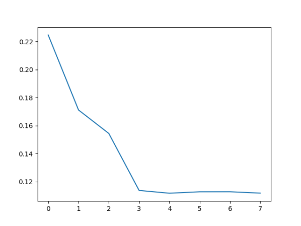
Cost

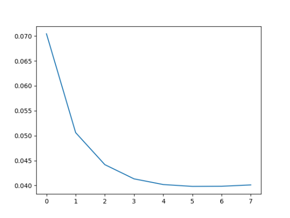
EPE3D

Figure 3: Curves of the cost and EPE3D error with respect to the iterations on the Flyingthigs3D dataset. As the alternate optimization progresses, the cost drops step by step, while the EPE3d error is decreased gradually.

3.3 Point-wise Optimization

Given the solution $\mathcal{X}^{k-1}=\{{\bm{x}}_{{1}}^{k-1},{\bm{x}}_{{2}}^{k-1},\cdots{\bm{x}}_{M}^{k-1}\}$ from the previous iteration, we first minimize Eq. (3) point-wisely to update $\mathcal{Z}^{k}$. The auxiliary transformation $\mathcal{Z}^{k}=\{{\bm{z}}_{{1}}^{k-1},{\bm{z}}_{{2}}^{k-1},\cdots{\bm{z}}_{M}^{k-1}\}$ contains the auxiliary flow vectors for each point in $\mathcal{P}$. An auxiliary flow vector ${\bm{z}}_{m}^{k}$ minimizes both the feature distance between ${\bm{f}}_{\mathcal{P}}({\bm{p}}_{m})$ and ${\bm{f}}_{\mathcal{Q}}({\bm{p}}_{m}+{\bm{z}}^{k}_{m})$ as well as the euclidean distance between ${\bm{z}}_{m}^{k}$ and ${\bm{x}}_{m}^{k-1}$:

$${\bm{z}}_{m}^{k}=\operatorname*{arg\,min}_{{\bm{z}}}\|{\bm{f}}_{\mathcal{P}}({\bm{p}}_{m})-{\bm{f}}_{\mathcal{Q}}({\bm{p}}_{m}+{\bm{z}})\|+\|{\bm{z}}-{\bm{x}}_{m}^{k-1}\|.$$ (5)

However, ${\bm{p}}_{m}+{\bm{z}}$ usually does not exactly correspond to any point ${\bm{q}}_{n}$ in $\mathcal{Q}$, so we use ${\bm{u}}_{n}={\bm{q}}_{n}-{\bm{p}}_{m}$ as a candidate for ${\bm{z}}_{m}^{k}$ and search for the best ${\bm{q}}_{n}$ within a local neighborhood $\Omega$ around ${\bm{p}}_{m}+{\bm{x}}_{m}^{k-1}$. This winer-take-all selection is further softened as a bilateral interpolation:

$$\footnotesize{\bm{z}}_{m}^{k}=\frac{1}{W}\sum_{{\bm{q}}_{n}\in\Omega}\exp(-\frac{\|{\bm{f}}_{\mathcal{P}}({\bm{p}}_{m})-{\bm{f}}_{\mathcal{Q}}({\bm{q}}_{n})\|}{\sigma_{{\bm{f}}}}-\frac{\|{\bm{u}}_{n}-{\bm{x}}_{m}^{k-1}\|}{\sigma_{{\bm{u}}}}){\bm{u}}_{n},$$ (6)

where $W$ is the normalization term that sum all the bilateral weights. Empirically, the reversed distance $-(\|{\bm{f}}_{\mathcal{P}}({\bm{p}}_{m})-{\bm{f}}_{\mathcal{Q}}({\bm{q}}_{n})\|)/\sigma_{{\bm{f}}})$ and $-(\|{\bm{u}}_{n}-{\bm{x}}_{m}^{k-1}\|)/\sigma_{{\bm{u}}}$ can be further replaced with cosine similarity for better performance, which converts Eq. (6) into:

$${\bm{z}}_{m}^{k}=\sum_{{\bm{q}}_{n}\in\Omega}\mathrm{softmax}({\bm{g}}^{\top}_{m}{\bm{g}}_{n}){\bm{u}}_{n},$$ (7)

where ${\bm{g}}_{m}$ concatenates ${\bm{f}}_{\mathcal{P}}({\bm{p}}_{m})$ and the positional encoding of ${\bm{p}}_{m}+{\bm{x}}_{m}^{k-1}$, while ${\bm{g}}_{n}$ concatenates ${\bm{f}}_{\mathcal{Q}}({\bm{q}}_{n})$ and the positional encoding of ${\bm{q}}_{n}$. Eq. (7) is similar to the attention  [58] mechanism, but uses the same feature operator for the key and the queries.

For point cloud registration, two additional steps are required. First, before Eq. (7), the point-wise flow vector ${\bm{x}}_{m}^{k-1}$ is calculated by the difference between ${\bm{p}}_{m}$ and its corresponding projection transformed by $\mathcal{X}^{k-1}=\{{\bm{Q}}^{k-1},{\bm{T}}^{k-1}\}$. Second, after ${\bm{z}}_{m}^{k}$ is estimated, the auxiliary 6-DOF transformation $\mathcal{Z}^{k}$ is computed via the PnP algorithm [13] from the auxiliary 3D flow vectors ${\bm{z}}_{1\cdots M}^{k}$.

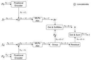
Figure 4: Details of point-wise optimization module. The positional encoder and the MLPs-attention blocks are both composed of two fully-connected layers. The parameters of these two blocks for point cloud $\mathcal{P}$ and $\mathcal{Q}$ are shared. The residual block is to obtain the position residual of currently estimated points and their neighborhood points.

3.4 Recurrent Regularization

Given the auxiliary transformation $\mathcal{Z}^{k}$ from the last section, we further implicitly regularize $\mathcal{Z}^{k}$ into $\mathcal{X}^{k}$ by a recurrent network. The recurrent network receives previous iteration’s hidden state ${\bm{h}}_{k-1}$ and the current iteration information ${\bm{v}}_{k}=[{\bm{f}}_{\mathcal{P}}({\bm{p}}_{m})-{\bm{f}}_{\mathcal{Q}}({\bm{p}}_{m}+{\bm{x}}_{m}^{k-1}),{\bm{z}}_{m}^{k}]$ as the inputs, where ${\bm{f}}_{\mathcal{Q}}({\bm{p}}_{m}+{\bm{x}}_{m}^{k-1})$ is interpolated similarly to Eq. (7). Then an updated hidden state ${\bm{h}}_{k}$ is produced from a recurrent unit such as GRU [7] as follows:

$${\bm{w}}_{k} =\sigma(set\_conv_{\bm{w}}([{\bm{h}}_{k-1},{\bm{v}}_{k}])),$$ (8)

$${\bm{r}}_{k} =\sigma(set\_conv_{\bm{r}}([{\bm{h}}_{k-1},{\bm{v}}_{k}])),$$

$$\tilde{{\bm{h}}}_{k} =\tanh(set\_conv_{\bm{h}}([{\bm{r}}_{k}\odot{\bm{h}}_{k-1},{\bm{v}}_{k}])),$$

$${\bm{h}}_{k} =(1-{\bm{w}}_{k})\odot{\bm{h}}_{k-1}+{\bm{w}}_{k}\odot\tilde{{\bm{h}}}_{k},$$

where $\odot$ is the element-wise product, $[\cdot,\cdot]$ is a concatenation and $\sigma(\cdot)$ is the sigmoid activation function. To initialize the first iteration’s hidden state ${\bm{h}}_{0}$, we set $\mathcal{Z}^{1}=\mathcal{X}_{0}$ and pass ${\bm{v}}_{1}$ through two $set\_conv$ layers.

After the new hidden state ${\bm{h}}_{k}$ has been produced, we use a transformation predictor consisting of two $set\_conv$ layers to estimate the residual $\Delta\mathcal{Z}^{k}$ between $\mathcal{Z}^{k}$ and the regularized transformation $\mathcal{X}^{k}$, and update the transformation as $\mathcal{X}^{k}=\mathcal{Z}^{k}+\Delta\mathcal{Z}^{k}$. For point cloud registration, we additionally max-pool the hidden state ${\bm{h}}_{k}$ overall points, and predict the residual 6-DOF transformation $\Delta\mathcal{Z}^{k}$ from the max-pooled feature vector, and update the transformation in $SE(3)$ manifold as $\mathcal{X}^{k}=\Delta\mathcal{Z}^{k}\otimes\mathcal{Z}^{k}$.

4 Training Loss

Similar to previous methods [64, 27], our networks can be trained in either a supervised way or a self-supervised way.

4.1 Supervised Training

In the training of the scene flow network, given the ground truth 3D flow vectors$\{{\bm{x}}^{*}_{{\bm{p}}_{i}}\}$ at each point ${\bm{p}}_{i}$, the $L_{1}$ loss is adopted as:

$$\mathcal{L}_{flow}=\frac{1}{M}\sum_{i}\|\hat{{\bm{x}}}_{{\bm{p}}_{i}}-{\bm{x}}^{*}_{{\bm{p}}_{i}}\|,$$ (9)

where $\{\hat{{\bm{x}}}_{{\bm{p}}_{i}}\}$ is the predicted flow from the recurrent regularization in the last iteration.

In the training of the point cloud registration network, we first transform the source point cloud $\mathcal{P}$ with the ground-truth transformation $\{{\bm{Q}}^{*},{\bm{T}}^{*}\}$ and the predicted transformation $\hat{{\bm{Q}}},\hat{{\bm{T}}}$ respectively, and then compute the difference between the transformed point clouds as:

$$\mathcal{L}_{register}=\frac{1}{M}\sum_{i}\|(\hat{{\bm{Q}}}\cdot{\bm{p}}_{i}+\hat{{\bm{T}}})-({\bm{Q}}^{*}\cdot{\bm{p}}_{i}+{\bm{T}}^{*})\|.$$ (10)

4.2 Self-supervised Training

The ground truth 3D flow is expensive, so the network needs to utilize the geometric priors as supervision when there is no access to the ground truth. Following previous work [64], our self-supervised loss for scene flow is composed of three terms: Chamfer distance, Smoothness regularization, and Laplacian regularization [60, 49].

Chamfer Term

The Chamfer distance enforces the source point cloud $\mathcal{P}$ to move close to the target point cloud $\mathcal{Q}$ with the mutual closest points as:

$$\mathcal{L}_{C}= \sum_{{\bm{p}}_{i}\in\mathcal{P}^{\prime}}\min_{{\bm{q}}_{j}\in\mathcal{Q}}\|{\bm{p}}_{i}-{\bm{q}}_{j}\|_{2}^{2}+\sum_{{\bm{q}}_{j}\in\mathcal{Q}}\min_{{\bm{p}}_{i}\in\mathcal{P}^{\prime}}\|{\bm{q}}_{j}-{\bm{p}}_{i}\|_{2}^{2},$$ (11)

where $\mathcal{P}^{\prime}$ is transformed from $\mathcal{P}$ by the predicted 3D flow vectors.

Smoothness Term

The smoothness constraint encourages the adjacent points to have similar 3D flow predictions as:

$$\mathcal{L}_{S}=\sum_{i}\frac{1}{|L({\bm{p}}_{i})|}\sum_{{\bm{p}}_{j}\in L({\bm{p}}_{i})}||\hat{{\bm{x}}}_{{\bm{p}}_{j}}-\hat{{\bm{x}}}_{{\bm{p}}_{i}}||_{2}^{2},$$ (12)

where $L({\bm{p}}_{i})$ is the local neighbor region of ${\bm{p}}_{i}$, and $|L({\bm{p}}_{i})|$ it the number of points in this local region.

Laplacian Term

The Laplacian coordinate vector approximates the local shape and curvature around a point ${\bm{p}}_{i}$ as:

$$\delta_{i}=\sum_{i}\frac{1}{|L({\bm{p}}_{i})|}\sum_{{\bm{p}}_{j}\in L({\bm{p}}_{i})}({\bm{p}}_{j}-{\bm{p}}_{i}).$$ (13)

Ideally, the transformed point cloud $\mathcal{P}^{\prime}$ should have the same Laplacian coordinate with the target point cloud $\mathcal{Q}$. So we adopt a regularization term based on the Laplacian coordinate similar to [64], as:

$$\mathcal{L}_{R}=\sum_{{\bm{p}}_{i}^{\prime}\in\mathcal{P}^{\prime}}\|\delta({\bm{p}}_{i}^{\prime})-\delta({\bm{q}}_{inter})\|_{2}^{2},$$ (14)

where $\delta({\bm{q}}_{inter})$ is the interpolated Laplacian coordinate from point cloud $Q$ at the same position as ${\bm{p}}_{i}^{\prime}$.

In summary, the self-supervised loss for the scene flow is defined as the weighted sum of these three terms, as:

$$\mathcal{L}_{selflow}=\alpha_{1}\mathcal{L}_{C}+\alpha_{2}\mathcal{L}_{S}+\alpha_{3}\mathcal{L}_{R}.$$ (15)

Datasets	Method	Sup.	EPE3D$\downarrow$	Acc3DS$\uparrow$	AccDR$\uparrow$	Outliers3D$\downarrow$
FlyingThings3D	ICP[4]	Self	$0.4062$	$0.1614$	$0.3038$	$0.8796$
	Ego-motion[53]	Self	$0.1696$	$0.2532$	$0.5501$	$0.8046$
	PointPWC-Net[64]	Self	$0.1246$	$0.3068$	$0.6552$	$0.7032$
	FlowStep3D[27]	Self	$0.0852$	$0.5363$	$0.8262$	$0.4198$
	Ours	Self	$\mathbf{0.0765}$	$\mathbf{0.5858}$	$\mathbf{0.8602}$	$\mathbf{0.4142}$
	FlowNet3D[30]	Full	$0.1136$	$0.4125$	$0.7706$	$0.6016$
	HPLFlowNet[18]	Full	$0.0804$	$0.6144$	$0.8555$	$0.4287$
	PointPWC-Net[64]	Full	$0.0588$	$0.7379$	$0.9276$	$0.3424$
	FLOT[37]	Full	$0.0520$	$0.7320$	$0.9270$	$0.3570$
	FlowStep3D [27]	Full	$0.0455$	$0.8162$	$0.9614$	$0.2165$
	Ours	Full	$\mathbf{0.0403}$	$\mathbf{0.8567}$	$\mathbf{0.9635}$	$\mathbf{0.1976}$
KITTI	ICP[4]	Self	$0.5181$	$0.0669$	$0.1667$	$0.8712$
	Ego-motion[53]	Self	$0.4154$	$0.2209$	$0.3721$	$0.8096$
	PointPWC-Net[64]	Self	$0.2549$	$0.2379$	$0.4957$	$0.6863$
	FlowStep3D[27]	Self	$0.1021$	$0.7080$	$0.8394$	$0.2456$
	Ours	Self	$\mathbf{0.0763}$	$\mathbf{0.7856}$	$\mathbf{0.8921}$	$\mathbf{0.1849}$
	FlowNet3D[30]	Full	$0.1767$	$0.3738$	$0.6677$	$0.5271$
	HPLFlowNet[18]	Full	$0.1169$	$0.4783$	$0.7776$	$0.4103$
	PointPWC-Net[64]	Full	$0.0694$	$0.7281$	$0.8884$	$0.2648$
	FLOT[37]	Full	$0.0560$	$0.7550$	$0.9080$	$0.2420$
	FlowStep3D [27]	Full	$0.0546$	$0.8051$	$0.9254$	$0.1492$
	Ours	Full	$\mathbf{0.0481}$	$\mathbf{0.8491}$	$\mathbf{0.9448}$	$\mathbf{0.1228}$

Table 1: Evaluation results on the FlyingThings3D [32] and KITTI [33] datasets. “Self" denotes training under the self-supervised setting while “Full" denotes under the supervised setting. All methods are only trained on FlyingThings3D [32]. In default setting, we set the iteration number to 7 and 14 for FlyingThings3D [32] and KITTI [33], respectively.

5 Experiments

5.1 3D Flow Estimation

Dataset

To make a fair comparison, we follow previous works [30, 64, 37, 27] to evaluate all participating methods on FlyingThings3D [32] and KITTI [33] for 3D flow estimation. The FlyingThings3D is a synthetic dataset that is rendered from scenes with multiple randomly sampled moving objects from the ShapeNet[5] dataset. It contains around 32k stereo images with ground truth disparity and optical flow maps. To use it for 3D flow estimation, we post-process it as in [64] into 19640 training pairs and 3824 testing pairs of point clouds, and each point cloud contains 8192 3D points on average. Similarly, the KITTI scene flow dataset [33] is also originally designed to evaluate the image based methods. We follow [64] and post-process it into 142 testing pairs only for evaluation.

Training Details

We train and evaluate our method with both the self-supervised and the supervised setting as described in Sec.4. To speed up the training, we adopt a two-stage training strategy: first, we set the batch size to 8 on 4 GTX 2080Ti GPUs, and alternate between the Eq. (7) and the Eq. (LABEL:equ:recurrent) for 3 times. The learning rate adopts the step decay strategy, where the initial learning rate is set to 1e-3 and then halved every 25 epochs, and 90 epochs were trained in total; second, we fine-tune the trained model from the first stage, but iterate more times and train for fewer epochs. We reduce the batch size to 4 to enable 7 iterations of Eq. (7) and Eq. (LABEL:equ:recurrent). The initial learning rate is also reduced to 1.25e-4 and then decayed every 5 epochs, and the model is trained for 10 epochs.

Quantitative Comparisons

We follow previous works [30, 64, 37, 27] to use the following metrics for evaluation:

1. EPE3D (m): $\sum||F_{pred}-F_{gt}||_{2}/N$ average distance error of all predicted values

2. Acc3DS: the percentage of points which statisfied $||F_{pred}-F_{gt}||_{2}<0.05m$ or $||F_{pred}-F_{gt}||_{2}/F_{gt}<5\%$

3. Acc3DR: the percentage of points which statisfied $||F_{pred}-F_{gt}||_{2}<0.1m$ or $||F_{pred}-F_{gt}||_{2}/F_{gt}<10\%$

4. Outliers3D: the percentage of points which statisfied $||F_{pred}-F_{gt}||_{2}>0.3m$ or $||F_{pred}-F_{gt}||_{2}/F_{gt}>10\%$.

As shown in Tab. 1, we have achieved state-of-the-art results for both self-supervised and supervised setting. Specifically, we performs better than the other methods by a large margin on the KITTI dataset, which demonstrates the superiority of our formulation in Eq. (7).

Method	MAE(R)	MAE(t)	Error(R)	Error(t)
ICP[4]	$13.719$	$0.132$	$27.250$	$0.280$
RPM[17]	$9.771$	$0.092$	$19.551$	$0.212$
FGR[71]	$19.266$	$0.090$	$30.839$	$0.192$
PointNetLK[1]	$15.931$	$0.142$	$29.725$	$0.297$
DCP-v2[62]	$6.380$	$0.083$	$12.607$	$0.169$
TEASER++[66]	$4.138$	$0.020$	$7.144$	$0.041$
RPMNet[69]	$0.893$	$0.0087$	$1.712$	$0.018$
Ours	$\mathbf{0.845}$	$\mathbf{0.0077}$	$\mathbf{1.665}$	$\mathbf{0.016}$

Table 2: Evaluation results on ModelNet40 [65] on partially visible setting with Gaussian noise.

 

 

 

 

 

PC1 and PC2

PC1+GT and PC2

PC1+Pred and PC2

Error

Figure 5: Qualitative results on the KITTI [33] scene flow dataset.

Iterations	KITTI				FlyingThings3D
	EPE3D$\downarrow$	Acc3DS$\uparrow$	AccDR$\uparrow$	Outliers3D$\downarrow$	EPE3D$\downarrow$	Acc3DS$\uparrow$	AccDR$\uparrow$	Outliers3D$\downarrow$
0	$0.1696$	$0.2744$	$0.5967$	$0.5671$	$0.1277$	$0.1809$	$0.6127$	$0.7428$
3	$0.0660$	$0.7513$	$0.8877$	$0.1893$	$0.0460$	$0.80720$	$0.9517$	$0.2476$
7	$0.0570$	$0.7979$	$0.9154$	$0.1566$	$0.0403$	$0.8567$	$0.9635$	$0.1976$
10	$0.0521$	$0.8245$	$0.9299$	$0.1385$	$0.0409$	$0.8532$	$0.9631$	$0.2035$
14	$0.0481$	$0.8491$	$0.9448$	$0.1228$	$0.0429$	$0.8368$	$0.9606$	$0.2227$

Table 3: Ablation studies of iterations.

Input

iter=0

iter=1

iter=3

iter=9

iter=14

Figure 6: Visualization of different iterations. As the number of iterations increases, two point clouds from KITTI[33] scene flow dataset are gradually aligned together.

5.2 Point Cloud Registration

Dataset

We follow previous methods [69] to evaluate on the ModelNet40 [65] dataset which contains 40 object categories of CAD models. Each CAD model is sampled into 2048 points and normalized into a unit sphere as in [69]. In order to generate training pairs with ground-truth rigid transformations, we follow RPMNet[69] to first synthetic transformation and then transform an existing source point cloud to the target point cloud. The transformation is synthesized by randomly sampling the rotation vector between $[0^{\circ},45^{\circ}]$ and the translation vector between $[-0.5,0.5]$. To simulate the condition of partial-to-partial registration, $30\%$ of the points are further removed according to a random direction [69]. We use the first 20 categories for training and validation and the remained 20 categories for evaluation.

Training Details

Compared with the FlyingThings3D, the ModelNet40 is a relatively small scale dataset, so we train our model for point cloud registration in a single stage, where the batch size is 8 on each GPU, and alternate between the Eq. (7) and the Eq. (LABEL:equ:recurrent) for 7 times. The learning rate also adopts the same decay strategy as above and is decayed every 100 epochs, while the model is trained 600 epochs.

Quantitative Comparisons

The quantitative comparisons follow previous works and use both the isotropic metrics $Error(R)$ and $Error(t)$ [69] as well as the anisotropic metric $MAE(R)$ and $MAE(t)$ [62]:

1. $Error(R)$: $arcos\frac{tr({R_{gt}}^{-1}R_{pred}-1)}{2}$

2. $Error(t)$: $||R_{gt}^{-1}t-t_{gt}||_{2}$

3. $MAE(R)$: $||Euler(R_{gt})-Euler(R_{pred})||_{1}$

4. $MAE(t)$: $||R_{gt}^{-1}t-t_{gt}||_{1}$.

As shown in Tab. 2, our method outperforms previous methods on both isotropic metrics and anisotropic metrics.

5.3 Ablation Studies

In order to further analyze the effectiveness of each component, we conduct ablation studies on 3D flow estimation and evaluate different variations of our model.

Point-wise Optimization

The first question is whether we need to further update the transformation after the recurrent regularization, i.e., can we remove the point-wise optimization Eq. (7) and only preserve the recurrent regularization Eq. (LABEL:equ:recurrent) to answer this question, we exclude Eq. (7) for both training and inference, which performs significantly worse as shown in the first row of Tab. 4 and indicate that the point-wise optimization is necessary. We also explore different alternative options for point-wise optimization. First, we only optimize the feature metric distance and do not constrain the difference between the auxiliary variable $\mathcal{Z}$ and $\mathcal{X}$. As shown in the second row of Tab. 4, the result is even worse than not using Eq. (7), which is because the feature distance only is ambiguous in some regions such as planar areas. Second, we use Eq. (5) directly instead of the soften version Eq. (7). We train the model with Gumbel Softmax and inference with argmax. The Gumbel Softmax performs worse than the soften version in Eq. (7), which is because the gradient back-propagated by the Eq. (7) is less noisy for training. Additionally, we also evaluate Eq. (6) using bilateral weight, which performs worse than Eq. (7). Therefore, we use Eq. (7) as the default setting to minimize Eq. (5) point-wisely.

Point-wise Optimization	EPE3D$\downarrow$	Acc3DS$\uparrow$	AccDR$\uparrow$	Outliers3D$\downarrow$
W/O	$0.0514$	$0.7612$	$0.9308$	$0.2880$
Feature Only	$0.0445$	$0.8327$	$0.9614$	$0.2318$
Gumbel Softmax	$0.0451$	$0.8262$	$0.9604$	$0.2370$
Bilateral Weight	$0.0441$	$0.8361$	$0.9555$	$0.2305$
Ours	$0.0403$	$0.8567$	$0.9635$	$0.1976$

Table 4: Ablation studies of point-wise optimization module. We show some alternative ways.

Recurrent Regularization

The second question is whether we need to solve Eq. (4) with a recurrent network, i.e., can we use standard point convolution? We replace the GRU [7] block with three $set\_conv$ [39] layers to keep similar model parameters for fair comparison, which increases the EPE3D from $0.0405$ to $0.0491$ as shown in Tab. 5. It indicates that the historical information passed by the recurrent unit regularizes the solution better. We also replace the GRU [7] unit with LSTM [22], which has slight improvement in Tab. 5. Therefore, we use GRU [7] as our default recurrent unit because of its simpler formulation.

Recurrent Reg.	EPE3D$\downarrow$	Acc3DS$\uparrow$	AccDR$\uparrow$	Outliers3D$\downarrow$
Set_Conv [39]	$0.0491$	$0.7682$	$0.9408$	$0.2823$
GRU [7]	$0.0403$	$0.8567$	$0.9635$	$0.1976$
LSTM [22]	$0.0402$	$0.8578$	$0.9642$	$0.1991$

Table 5: Ablation studies of recurrent regularization module. We use GRU [7] as our default recurrent unit because of the simple formulation.

Number of Iterations:

During training, the final iteration number of Eq. (7) and Eq. (LABEL:equ:recurrent) is 7. While during inference, we vary the iteration number from 3 to 14 to investigate how the performance changes along with the iteration number. As shown in Tab. 3, for the KITTI [33] dataset, all the metrics are gradually improved along with the increasing iteration number. However, for the FlyingThings3D[32] dataset, the performance reaches the peak when the iteration number is exactly the same as training, and gradually degrades afterward. It is because FlyingThings3D [32] is more challenging because of its larger motion and more complicated occlusion than KITTI [33]. Therefore, we set the iteration number to 7 for Flyingthings3D [32] and 14 for KITTI [33] as the default setting.

6 Conclusion

We propose a recurrent framework for the 3D motion estimation. To address the irregularity of the point cloud, we optimize the 3D flows on a point-wise cost. Then a recurrent network globally regularize the flow to output an accurate 3D motion estimation. We generalize our method to both the 3D scene flow estimation task and the point cloud registration task. The experiments demonstrate that our method outperforms previous methods and achieves a new state-of-the-art performance across all metrics.

References

- [1] Yasuhiro Aoki, Hunter Goforth, Rangaprasad Arun Srivatsan, and Simon Lucey. PointNetLK: Robust & efficient point cloud registration using pointnet. In IEEE Conference on Computer Vision and Pattern Recognition (CVPR), pages 7163–7172, 2019.
- [2] A. Behl, Despoina Paschalidou, S. Donné, and A. Geiger. Pointflownet: Learning representations for rigid motion estimation from point clouds. 2019 IEEE/CVF Conference on Computer Vision and Pattern Recognition (CVPR), pages 7954–7963, 2019.
- [3] Paul J Besl and Neil D McKay. Method for registration of 3-d shapes. In Sensor fusion IV: control paradigms and data structures, volume 1611, pages 586–606. International Society for Optics and Photonics, 1992.
- [4] Paul J. Besl and Neil D. McKay. A method for registration of 3-d shapes. IEEE Transactions on Pattern Analysis and Machine Intelligence (TPAMI), 14(2):239–256, 1992.
- [5] Angel X Chang, Thomas Funkhouser, Leonidas Guibas, Pat Hanrahan, Qixing Huang, Zimo Li, Silvio Savarese, Manolis Savva, Shuran Song, Hao Su, et al. Shapenet: An information-rich 3d model repository. arXiv preprint arXiv:1512.03012, 2015.
- [6] Hui Chen and Bir Bhanu. 3D free-form object recognition in range images using local surface patches. Pattern Recognition Letters, 28(10):1252–1262, 2007.
- [7] Kyunghyun Cho, Bart Van Merriënboer, Caglar Gulcehre, Dzmitry Bahdanau, Fethi Bougares, Holger Schwenk, and Yoshua Bengio. Learning phrase representations using rnn encoder-decoder for statistical machine translation. arXiv preprint arXiv:1406.1078, 2014.
- [8] Haili Chui and Anand Rangarajan. A feature registration framework using mixture models. In IEEE Workshop on Mathematical Methods in Biomedical Image Analysis. MMBIA-2000 (Cat. No. PR00737), pages 190–197. IEEE, 2000.
- [9] Marco Cuturi. Sinkhorn distances: Lightspeed computation of optimal transport. Advances in neural information processing systems, 26, 2013.
- [10] Haowen Deng, Tolga Birdal, and Slobodan Ilic. PPFNet: Global context aware local features for robust 3D point matching. In IEEE Conference on Computer Vision and Pattern Recognition (CVPR), 2018.
- [11] Ayush Dewan, Tim Caselitz, Gian Diego Tipaldi, and Wolfram Burgard. Rigid scene flow for 3d lidar scans. In Proceedings of the IEEE/RSJ International Conference on Intelligent Robots and Systems, pages 1765–1770. IEEE, 2016.
- [12] Zhen Dong, Bisheng Yang, Yuan Liu, Fuxun Liang, Bijun Li, and Yufu Zang. A novel binary shape context for 3d local surface description. ISPRS Journal of Photogrammetry and Remote Sensing, 130:431–452, 2017.
- [13] Martin A Fischler and Robert C Bolles. Random sample consensus: a paradigm for model fitting with applications to image analysis and automated cartography. Communications of the ACM, 24(6):381–395, 1981.
- [14] Andrea Frome, Daniel Huber, Ravi Kolluri, Thomas Bülow, and Jitendra Malik. Recognizing objects in range data using regional point descriptors. In European Conference on Computer Vision (ECCV), pages 224–237. Springer, 2004.
- [15] Kexue Fu, Shaolei Liu, Xiaoyuan Luo, and Manning Wang. Robust point cloud registration framework based on deep graph matching. In Proceedings of the IEEE/CVF Conference on Computer Vision and Pattern Recognition, pages 8893–8902, 2021.
- [16] Guy Godin, Marc Rioux, and Rejean Baribeau. Three-dimensional registration using range and intensity information. In Sabry F. El-Hakim, editor, Videometrics III, volume 2350, pages 279 – 290. International Society for Optics and Photonics, SPIE, 1994.
- [17] Steven Gold, Anand Rangarajan, Chien-Ping Lu, Suguna Pappu, and Eric Mjolsness. New algorithms for 2d and 3d point matching: pose estimation and correspondence. Pattern recognition, 31(8):1019–1031, 1998.
- [18] Xiuye Gu, Y. Wang, Chongruo Wu, Y. Lee, and Panqu Wang. Hplflownet: Hierarchical permutohedral lattice flownet for scene flow estimation on large-scale point clouds. 2019 IEEE/CVF Conference on Computer Vision and Pattern Recognition (CVPR), pages 3249–3258, 2019.
- [19] Xiaodong Gu, Weihao Yuan, Zuozhuo Dai, Chengzhou Tang, Siyu Zhu, and Ping Tan. Dro: Deep recurrent optimizer for structure-from-motion. arXiv preprint arXiv:2103.13201, 2021.
- [20] Yulan Guo, Mohammed Bennamoun, Ferdous Sohel, Min Lu, Jianwei Wan, and Ngai Ming Kwok. A comprehensive performance evaluation of 3D local feature descriptors. International Journal of Computer Vision, 116(1):66–89, 2016.
- [21] S. Hadfield and R. Bowden. Kinecting the dots: Particle based scene flow from depth sensors. In 2011 International Conference on Computer Vision, pages 2290–2295, 2011.
- [22] Sepp Hochreiter and Jürgen Schmidhuber. Long short-term memory. Neural computation, 9(8):1735–1780, 1997.
- [23] Shengyu Huang, Zan Gojcic, Mikhail Usvyatsov, Andreas Wieser, and Konrad Schindler. Predator: Registration of 3d point clouds with low overlap. In Proceedings of the IEEE/CVF Conference on Computer Vision and Pattern Recognition, pages 4267–4276, 2021.
- [24] F. Huguet and F. Devernay. A variational method for scene flow estimation from stereo sequences. In 2007 IEEE 11th International Conference on Computer Vision, pages 1–7, 2007.
- [25] Eddy Ilg, Nikolaus Mayer, Tonmoy Saikia, Margret Keuper, Alexey Dosovitskiy, and Thomas Brox. Flownet 2.0: Evolution of optical flow estimation with deep networks. In Proceedings of the IEEE conference on computer vision and pattern recognition, pages 2462–2470, 2017.
- [26] Andrew E Johnson and Martial Hebert. Using spin images for efficient object recognition in cluttered 3d scenes. IEEE Transactions on pattern analysis and machine intelligence, 21(5):433–449, 1999.
- [27] Yair Kittenplon, Yonina C Eldar, and Dan Raviv. Flowstep3d: Model unrolling for self-supervised scene flow estimation. In Proceedings of the IEEE/CVF Conference on Computer Vision and Pattern Recognition, pages 4114–4123, 2021.
- [28] Jiaxin Li and Gim Hee Lee. USIP: Unsupervised stable interest point detection from 3d point clouds. In International Conference on Computer Vision (ICCV), 2019.
- [29] Y. Li, M. Tofighi, V. Monga, and Y. C. Eldar. An algorithm unrolling approach to deep image deblurring. In ICASSP 2019 - 2019 IEEE International Conference on Acoustics, Speech and Signal Processing (ICASSP), pages 7675–7679, 2019.
- [30] Xingyu Liu, Charles R Qi, and Leonidas J Guibas. Flownet3d: Learning scene flow in 3d point clouds. In Proceedings of the IEEE Conference on Computer Vision and Pattern Recognition, pages 529–537, 2019.
- [31] Weixin Lu, Guowei Wan, Yao Zhou, Xiangyu Fu, Pengfei Yuan, and Shiyu Song. DeepICP: An end-to-end deep neural network for 3D point cloud registration. In International Conference on Computer Vision (ICCV), 2019.
- [32] Nikolaus Mayer, Eddy Ilg, Philip Hausser, Philipp Fischer, Daniel Cremers, Alexey Dosovitskiy, and Thomas Brox. A large dataset to train convolutional networks for disparity, optical flow, and scene flow estimation. In Proceedings of the IEEE Conference on Computer Vision and Pattern Recognition (CVPR), June 2016.
- [33] Moritz Menze, Christian Heipke, and Andreas Geiger. Joint 3d estimation of vehicles and scene flow. In Proc. of the ISPRS Workshop on Image Sequence Analysis (ISA), 2015.
- [34] Vishal Monga, Yuelong Li, and Yonina C Eldar. Algorithm unrolling: Interpretable, efficient deep learning for signal and image processing. arXiv preprint arXiv:1912.10557, 2019.
- [35] Yue Pan, Bisheng Yang, Fuxun Liang, and Zhen Dong. Iterative global similarity points: A robust coarse-to-fine integration solution for pairwise 3d point cloud registration. In 2018 International Conference on 3D Vision (3DV), pages 180–189. IEEE, 2018.
- [36] François Pomerleau, Francis Colas, and Roland Siegwart. A review of point cloud registration algorithms for mobile robotics. Foundations and Trends in Robotics, 4(1):1–104, 2015.
- [37] Gilles Puy, Alexandre Boulch, and Renaud Marlet. Flot: Scene flow on point clouds guided by optimal transport. In European conference on computer vision, pages 527–544. Springer, 2020.
- [38] Charles R Qi, Hao Su, Kaichun Mo, and Leonidas J Guibas. Pointnet: Deep learning on point sets for 3d classification and segmentation. In Proceedings of the IEEE conference on computer vision and pattern recognition, pages 652–660, 2017.
- [39] Charles Ruizhongtai Qi, Li Yi, Hao Su, and Leonidas J Guibas. Pointnet++: Deep hierarchical feature learning on point sets in a metric space. In Advances in neural information processing systems, pages 5099–5108, 2017.
- [40] Szymon Rusinkiewicz. A symmetric objective function for icp. ACM Transactions on Graphics (TOG), 38(4):1–7, 2019.
- [41] Szymon Rusinkiewicz and Marc Levoy. Efficient variants of the icp algorithm. In Proceedings third international conference on 3-D digital imaging and modeling, pages 145–152. IEEE, 2001.
- [42] Radu Bogdan Rusu, Nico Blodow, and Michael Beetz. Fast point feature histograms (FPFH) for 3D registration. In IEEE International Conference on Robotics and Automation (ICRA), pages 3212–3217, 2009.
- [43] Radu Bogdan Rusu, Nico Blodow, Zoltan Csaba Marton, and Michael Beetz. Aligning point cloud views using persistent feature histograms. In IEEE/RSJ International Conference on Intelligent Robots and Systems (IROS), pages 3384–3391, 2008.
- [44] Samuele Salti, Federico Tombari, and Luigi Di Stefano. Shot: Unique signatures of histograms for surface and texture description. Computer Vision and Image Understanding, 125:251–264, 2014.
- [45] Paul-Edouard Sarlin, Daniel DeTone, Tomasz Malisiewicz, and Andrew Rabinovich. Superglue: Learning feature matching with graph neural networks. In Proceedings of the IEEE/CVF conference on computer vision and pattern recognition, pages 4938–4947, 2020.
- [46] Vinit Sarode, Xueqian Li, Hunter Goforth, Yasuhiro Aoki, Rangaprasad Arun Srivatsan, Simon Lucey, and Howie Choset. PCRNet: Point cloud registration network using pointnet encoding. In International Conference on Computer Vision (ICCV), 2019.
- [47] Aleksandr Segal, Dirk Haehnel, and Sebastian Thrun. Generalized-icp. In Robotics: science and systems, volume 2, page 435. Seattle, WA, 2009.
- [48] Richard Sinkhorn. A relationship between arbitrary positive matrices and doubly stochastic matrices. The annals of mathematical statistics, 35(2):876–879, 1964.
- [49] Olga Sorkine. Laplacian Mesh Processing. In Yiorgos Chrysanthou and Marcus Magnor, editors, Eurographics 2005 - State of the Art Reports. The Eurographics Association, 2005.
- [50] Frank Steinbrücker, Thomas Pock, and Daniel Cremers. Large displacement optical flow computation withoutwarping. In 2009 IEEE 12th International Conference on Computer Vision, pages 1609–1614. IEEE, 2009.
- [51] Deqing Sun, Xiaodong Yang, Ming-Yu Liu, and Jan Kautz. Pwc-net: Cnns for optical flow using pyramid, warping, and cost volume. In Proceedings of the IEEE conference on computer vision and pattern recognition, pages 8934–8943, 2018.
- [52] Zachary Teed and Jia Deng. Raft: Recurrent all-pairs field transforms for optical flow. In European conference on computer vision, pages 402–419. Springer, 2020.
- [53] Ivan Tishchenko, Sandro Lombardi, Martin R Oswald, and Marc Pollefeys. Self-supervised learning of non-rigid residual flow and ego-motion. In 2020 International Conference on 3D Vision (3DV), pages 150–159. IEEE, 2020.
- [54] Federico Tombari, Samuele Salti, and Luigi Di Stefano. Unique shape context for 3D data description. In ACM Workshop on 3D Object Retrieval, 3DOR ’10, pages 57–62. ACM, 2010.
- [55] Yanghai Tsin and Takeo Kanade. A correlation-based approach to robust point set registration. In European Conference on Computer Vision (ECCV), pages 558–569. Springer, 2004.
- [56] Arash K Ushani and Ryan M Eustice. Feature learning for scene flow estimation from lidar. In Conference on Robot Learning, pages 283–292. PMLR, 2018.
- [57] Arash K Ushani, Ryan W Wolcott, Jeffrey M Walls, and Ryan M Eustice. A learning approach for real-time temporal scene flow estimation from lidar data. In Proceedings of the IEEE International Conference on Robotics and Automation, pages 5666–5673. IEEE, 2017.
- [58] Ashish Vaswani, Noam Shazeer, Niki Parmar, Jakob Uszkoreit, Llion Jones, Aidan N Gomez, Łukasz Kaiser, and Illia Polosukhin. Attention is all you need. In Advances in neural information processing systems, pages 5998–6008, 2017.
- [59] Sundar Vedula, Simon Baker, Peter Rander, Robert Collins, and Takeo Kanade. Three-dimensional scene flow. In Proceedings of the International Conference on Computer Vision, volume 2, pages 722–729. IEEE, 1999.
- [60] Nanyang Wang, Yinda Zhang, Zhuwen Li, Yanwei Fu, Wei Liu, and Yu-Gang Jiang. Pixel2mesh: Generating 3d mesh models from single rgb images. In Proceedings of the European Conference on Computer Vision (ECCV), pages 52–67, 2018.
- [61] Shenlong Wang, Simon Suo, Wei-Chiu Ma, Andrei Pokrovsky, and Raquel Urtasun. Deep parametric continuous convolutional neural networks. In Proceedings of the IEEE Conference on Computer Vision and Pattern Recognition, pages 2589–2597, 2018.
- [62] Yue Wang and Justin M. Solomon. Deep closest point: Learning representations for point cloud registration. In International Conference on Computer Vision (ICCV), 2019.
- [63] Yue Wang and Justin M Solomon. Prnet: Self-supervised learning for partial-to-partial registration. In Advances in Neural Information Processing Systems 32, pages 8814–8826. Curran Associates, Inc., 2019.
- [64] Wenxuan Wu, Zhi Yuan Wang, Zhuwen Li, Wei Liu, and Li Fuxin. Pointpwc-net: Cost volume on point clouds for (self-) supervised scene flow estimation. In European conference on computer vision, pages 88–107. Springer, 2020.
- [65] Zhirong Wu, Shuran Song, Aditya Khosla, Fisher Yu, Linguang Zhang, Xiaoou Tang, and Jianxiong Xiao. 3D ShapeNets: A deep representation for volumetric shapes. In IEEE Conference on Computer Vision and Pattern Recognition (CVPR), pages 1912–1920, 2015.
- [66] Heng Yang, Jingnan Shi, and Luca Carlone. Teaser: Fast and certifiable point cloud registration. IEEE Transactions on Robotics, 37(2):314–333, 2020.
- [67] Jiaolong Yang, Hongdong Li, Dylan Campbell, and Yunde Jia. Go-ICP: A globally optimal solution to 3D ICP point-set registration. IEEE Transactions on Pattern Analysis and Machine Intelligence (TPAMI), 38(11):2241–2254, 2015.
- [68] Zi Jian Yew and Gim Hee Lee. 3DFeat-Net: Weakly supervised local 3D features for point cloud registration. In European Conference on Computer Vision (ECCV). Springer, 2018.
- [69] Zi Jian Yew and Gim Hee Lee. Rpm-net: Robust point matching using learned features. In Proceedings of the IEEE/CVF conference on computer vision and pattern recognition, pages 11824–11833, 2020.
- [70] Andy Zeng, Shuran Song, Matthias Nießner, Matthew Fisher, Jianxiong Xiao, and Thomas Funkhouser. 3DMatch: Learning local geometric descriptors from RGB-D reconstructions. In IEEE Conference on Computer Vision and Pattern Recognition (CVPR), pages 199–208, 2017.
- [71] Qian-Yi Zhou, Jaesik Park, and Vladlen Koltun. Fast global registration. In European Conference on Computer Vision, pages 766–782. Springer, 2016.