Hierarchical dimensional crossover of an optically-trapped quantum gas with disorder

Abstract

Dimensionality serves as an indispensable ingredient in any attempt to formulate the low-dimensional physics, and studying the dimensional crossover at a fundamental level is challenging. The purpose of this work is to study the hierarchical dimensional crossovers, namely the crossover from three dimensions (3D) to quasi-2D and then to 1D. Our system consists of a 3D Bose-Einstein condensate (BEC) trapped in an anisotropic 2D optical lattice characterized by the lattice depths $V_{1}$ along the $x$ direction and $V_{2}$ along the $y$ direction, respectively, where the hierarchical dimensional crossover is controlled via $V_{1}$ and $V_{2}$. We analytically derive the ground-state energy, quantum depletion and the superfluid density of the system. Our results demonstrate the 3D-quasi-2D-1D dimensional crossovers in the behavior of quantum fluctuations. Conditions for possible experimental realization of our scenario are also discussed.

Key words: ultracold quantum gas, Bogoliubov theory, dimensional crossover, quantum depletion

Introduction.— Dimensionality plays a fundamental role in determining the properties of quantum many-body systems. It underpins many remarkable phenomena such as the high-Tc superconductivity Lee et al. (2006) and magic-angle graphene Cao et al. (2018a, b); Tarnopolsky et al. (2019) in two dimensions (2D) and the Tomonaga-Luttinger liquid Haldane (1981) in 1D. Therefore, there are ongoing interests and great efforts in investigating how dimensionality affects the properties of quantum many-body systems.

Tightly confined Bose-Einstein condensate (BEC) Bloch et al. (2008) provides an ideal playground for the theoretical and experimental explorations of the dimensional effects. In particular, the state-of-the-art technology allows the depth of an optical lattice to be arbitrarily tuned by changing the laser intensities, enabling realizations of quasi-1D Paredes et al. (2004) and quasi-2D Peppler et al. (2018); Holten et al. (2018) BECs. Thus, an important direction of investigation consists of studying the properties of a BEC system in the dimensional crossover.

Along this research line, many researches have been carried out. For instance, Refs. Orso et al. (2006); Hu et al. (2009) have shown that the presence of a 2D lattice can induce a 3D to 1D crossover in the behavior of quantum fluctuations; Refs. Hu and Liang (2011); Zhou et al. (2010); Faigle-Cedzich et al. (2021) have investigated quantum phases along the 3D-2D crossover and the visualization of the dimensional effects in collective excitations. These works Orso et al. (2006); Hu et al. (2009); Hu and Liang (2011); Zhou et al. (2010); Hu et al. (2019); Yin et al. (2020); Faigle-Cedzich et al. (2021); Yao et al. consider the tight confinement scheme that gives rise to a direct dimensional crossover from 3D to 2D or 1D (i.e., 3D-2D or 3D-1D crossover). Instead, we will be interested in the hierarchical dimensional crossovers, i.e., the 3D-quasi-2D-1D dimensional crossovers.

We will be interested in the effect of dimensionality on not only the ground state energy and quantum depletion but also the transport properties. This is motivated by experimental realizations of BECs in the presence of disorder White et al. (2009); Paiva et al. (2015). For example, superfluidity represents a kinetic property of a system, and the superfluid density is a transport coefficient determined by the linear response theory. In this work, we investigate the 3D - quasi-2D - 1D crossovers in the properties of a disorder BEC trapped in an anisotropic optical lattice, using the Green function approach. Specifically we calculate the ground-state energy and quantum depletion, as well as the superfluid density, and we analyze the combined effects of dimensionality and disorder.

Model.— At zero temperature, an optically-trapped BEC can be well described by the $N$-body Hamiltonian Orso et al. (2006); Hu et al. (2009); Hu and Liang (2011); Zhou et al. (2010)

$$\hat{H}-\mu\hat{N}=\int{\rm d}\bm{r}\hat{\Psi}^{\dagger}(\bm{r})\bigg{[}-\frac{\hbar^{2}\nabla^{2}}{2m}-\mu + V_{\text{opt}}(\bm{r})+V_{\text{ran}}(\bm{r})$$ (1)

$$+ \frac{g}{2}\hat{\Psi}^{\dagger}\hat{\Psi}\bigg{]}\hat{\Psi}(\bm{r}),$$

where $\hat{\Psi}(\bm{r})$ is the field operator for bosons with mass $m$, $\mu$ is the chemical potential, $\hat{N}=\int{\rm d}\bm{r}\hat{\Psi}^{\dagger}(\bm{r})\Psi(\bm{r})$ is the number operator, and $g=4\pi\hbar^{2}a_{\text{3}D}/m$ is the coupling constant with $a_{\text{3}D}$ being the 3D scattering length Petrov et al. (2000). In Hamiltonian (1), $V_{\text{opt}}(\bm{r})$ and $V_{\text{ran}}(\bm{r})$, respectively, describe the anisotropic 2D optical lattice and the external random potential.

We consider the anisotropic 2D optical lattice in Hamiltonian (1) in the form Bloch et al. (2008)

$$V_{\text{opt}}(\bm{r})=E_{R}[V_{1}\sin^{2}(q_{B}x)+V_{2}\sin^{2}(q_{B}y)],$$ (2)

where $V_{1,2}$ denote the laser intensities and $E_{R}=\hbar^{2}q_{B}^{2}/2m$ is the recoil energy, with $\hbar q_{B}$ being the Bragg momentum and $m$ the atomic mass. The lattice period is fixed by $d=\pi/q_{B}$. Atoms are free in the $z$ direction. By controlling the depths of the optical lattice $V_{1}$ and $V_{2}$, crossovers to low dimensions are expected to occur via the hierarchical access of new energy scales: firstly, a 3D Bose gas becomes quasi-2D when the energetic restriction to freeze $x$-direction excitations is reached; next, by further freezing the kinetic energy along the $y$-direction, the quasi-2D BEC is expected to enter the quasi-1D regime.

Moreover, in Hamiltonian (1), $V_{\text{ran}}(\bm{r})=\sum_{i}^{N_{\text{imp}}}v(\bm{r}-\bm{r}_{i})$ can be produced by the random potential Huang and Meng (1992); Hu et al. (2009); Zhou et al. (2010). For sufficiently dilute disorder White et al. (2009); Paiva et al. (2015), $v(\bm{r})$ can be approximated by an effective pseudopotential, i.e., $v(\bm{r})=g_{\text{imp}}\delta(\bm{r})$, where $g_{\rm{imp}}=2\pi\hbar^{2}\tilde{b}/m$ is the effective coupling constant of an impurity-boson pair and $\tilde{b}$ is the effective scattering length accounting for the presence of a 2D optical lattice Astrakharchik et al. (2002); Yao et al. (2020).

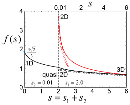
Figure 1: Scaling function $f(s)$ in Eq. (11) (black solid line) and its 3D (black dotted line) asymptotic behavior with $s=s_{1}+s_{2}$ being the dimensionless tunneling rates. In the left side of the vertical dashed line, we fix $s_{2}=0.01$ and set $s_{1}=[0,2]$. The blue dot denotes the 1D Lieb-Liniger limit of $f(0)=\frac{4\sqrt{2}}{3}$. In the right side, we fix $s_{1}=2$ and set $s_{2}=[0.01,4]$. As $s$ decreases from $6$ to $0$, the model system realizes the step-by-step dimensional crossover from 3D to quasi-2D and then 1D. In comparison, the red solid line denotes the one-step dimensional crossover from 3D to pure 2D studied in Ref. Zhou et al. (2010) with the red dotted curve being the pure 2D asymptotic behavior.

We assume the lattice depths $V_{1}$ and $V_{2}$ in Eq. (2) in unit of the recoil energy of $E_{R}$ are relatively large ($V_{1}\geq 5$, $V_{2}\geq 5$), so that the interband gap of $E_{\text{gap}}$ is bigger than the chemical potential of $\mu$, i. e. $E_{\text{gap}}\gg\mu$. Meanwhile, because of the quantum tunneling, the overlap of the wave functions of two consecutive wells are still sufficient to ensure full coherence even in the presence of disorder. By this assumption Orso et al. (2006); Hu et al. (2009); Hu and Liang (2011); Zhou et al. (2010), we restrict ourselves to the lowest band, where the physics is governed by the ratio between the chemical potential $\mu$ and the bandwith of $4(J_{1}+J_{2})$, where $J_{1}$ and $J_{2}$ are the tunneling rates between neighboring wells. Generally speaking, for $4(J_{1}+J_{2})\gg\mu$, the system retains an anisotropic 3D behavior, whereas for $4(J_{1}+J_{2})\simeq\mu$, the system undergoes a dimensional crossover to a 1D regime. In the limit of $4(J_{1}+J_{2})\ll\mu$, the model system can be treated as 1D. Following Refs. Orso et al. (2006); Hu et al. (2009); Hu and Liang (2011); Zhou et al. (2010), we treat our model system within the tight-binding approximation as shown in Appendix A. The lowest Bloch band of the model system can be described in terms of the Wannier functions as $\phi_{k_{x}}(x)\phi_{k_{y}}(y)$, with $\phi_{k_{x_{i}}}(x_{i})=\sum_{l}{\rm e}^{{\rm i}ldk_{x_{i}}}w(x_{i}-ld)$. Here, $w(x_{i})=\exp\left[-x_{i}^{2}/2\sigma_{i}^{2}\right]/\pi^{1/4}\sigma_{i}^{1/2}$ and $d/\sigma_{i}=\pi V_{i}^{1/4}\exp\left(-1/4\sqrt{V_{i}}\right)$ ($i=1,2$ and $x_{1}=x$, $x_{2}=y$). We remark that this work is limited into a tight-binding approximation by neglecting beyond-lowest-Bloch-band transverse modes along the $x$ and $y$ directions. Further considering the effects of beyond-lowest-Bloch-band transverse modes on the dimensional crossover goes beyond the scope of this work.

Directly following Refs. Hu et al. (2009); Zhou et al. (2010), we expand the field operators in Hamiltonian (1) as $\hat{\Psi}(\bm{r})=\sum_{\bm{k}}\hat{a}_{\bm{k}}{\rm e}^{-{\rm i}k_{z}z}\phi_{k_{x}}(x)\phi_{k_{y}}(y)$ and obtain

$$H-\mu N = \sum_{\bm{k}}\left(\varepsilon^{0}_{\bm{k}}-\mu\right)\hat{a}^{\dagger}_{\bm{k}}\hat{a}_{\bm{k}}+\frac{\tilde{g}}{2V}\sum_{\bm{k},\bm{q},{\bm{k}}^{\prime}}\hat{a}^{\dagger}_{\bm{k}+\bm{q}}\hat{a}^{\dagger}_{{\bm{k}}^{\prime}-{\bm{q}}}\hat{a}_{{\bm{k}}^{\prime}}\hat{a}_{\bm{k}}$$ (3)

$$+ \sum_{{\bm{k}},{\bm{k}}^{\prime}}\hat{a}^{\dagger}_{\bm{k}}\hat{a}_{\bm{k}^{\prime}}V_{\bm{k}-\bm{k}^{\prime}},$$

where

$$\varepsilon^{0}_{\bm{k}}=\frac{\hbar^{2}k_{z}^{2}}{2m}+2[J-J_{1}\cos k_{x}-J_{2}\cos k_{y}],$$ (4)

is the energy dispersion of the non-interacting system. Here, $J_{1}$ and $J_{2}$ are the tunneling rates along the $x$- and $y$-direction, respectively. Moreover, we have $J=J_{1}+J_{2}$, $V$ is the volume of the model system, and $\tilde{g}=gd^{2}/(2\pi\sigma_{1}\sigma_{2})$ is the renormalized coupling constant. The $V_{\bm{k}}=1/V\int{\rm e}^{{\rm i}{\bm{k}}\cdot{\bm{r}}}V_{\text{ran}}{\rm d}\bm{r}$ in Eq. (3) is the Fourier transform of disorder potential.

We remark that in this work, we do not consider the effect of the confinement-induced resonance (CIR) Peng et al. (2010); Zhang and Zhang (2011) on the coupling constant $\tilde{g}$. The basic physics of CIR can be understood in the language of Feshbach resonance Bergeman et al. (2003), where the scattering open channel and closed channels are, respectively, represented by the ground-state transverse mode and the other transverse modes along the tight-confinement dimensions. Within the tight-binding approximation assumed in this work, the ultracold atoms are frozen in the states of the lowest Bloch band and can not be excited into the other transverse modes. Thus the effect of CIR on $\tilde{g}$ can be safely ignored as the closed channels are absent Peng et al. (2010); Zhang and Zhang (2011); Bergeman et al. (2003).

Our subsequent calculations proceed in two steps. First, we calculate the ground state energy and quantum depletion. Previous studies Hu et al. (2009); Zhou et al. (2010) have shown that the effects of disorder simply lead to trivial energy shifts in the ground state energy, and therefore, we shall ignore the disorder potential in this part of calculations and set $V_{\text{ran}}=0$. Second, we investigate how the dimensionality affects the superfluid density in the presence of the disorder potential $V_{\text{ran}}\neq 0$.

Ground state energy and quantum depletion — For an optically-trapped Bose gas described by Hamiltonian (1), the ground state energy $E_{g}$ and quantum depletion can be calculated via the single-particle Green function $G(\bm{k},\omega)$ Souza et al. (2021) as follows

$$\frac{E_{g}}{V}\!=\!\frac{\tilde{g}n^{2}}{2}\!\!+\!\!\lim\limits_{t\rightarrow 0-}\!\!\frac{1}{(2\pi)^{3}d^{2}}\!\!\int\!\!{\rm d}k_{z}{\rm d}^{2}\bm{k}\!\!\int\!\!\frac{{\rm d}\omega}{2\pi{\rm i}}{\rm e}^{-{\rm i}\omega t}\!E_{\bm{k}}G(\bm{k},\omega),$$ (5)

$$\frac{N-N_{0}}{N}\!=\!\lim\limits_{t\rightarrow 0-}\frac{{\rm i}}{(2\pi)^{4}d^{2}n}\int{\rm d}k_{z}{\rm d}^{2}\bm{k}\int{\rm d}\omega{\rm e}^{-{\rm i}\omega t}G(\bm{k},\omega),$$ (6)

with $E(\bm{k})$ being the excitation energy. In Eqs. (5) and (6), the $G(\bm{k},\omega)$ is the Fourier transformation of the Green function

$$G(\bm{k},t-t^{\prime})=-{\rm i}\left\langle T\hat{a}_{\bm{k}}(t)\hat{a}_{\bm{k}}^{\dagger}(t^{\prime})\right\rangle,$$ (7)

in the Heisenberg representation, where $T$ denotes the chronological product.

By applying the Bogoliubov theory Orso et al. (2006); Hu et al. (2009); Hu and Liang (2011); Zhou et al. (2010); Faigle-Cedzich et al. (2021) to the Hamiltonian (1), we follow the standard procedures and obtain

$$G(\bm{k},\omega)=\frac{\omega+\varepsilon^{0}_{\bm{k}}+\tilde{g}n}{\omega^{2}-E^{2}_{\bm{k}}+{\rm i}0}.$$ (8)

Here, $n_{0}$ is the condensate density, $E_{\bm{k}}=\sqrt{\varepsilon^{0}_{\bm{k}}(\varepsilon^{0}_{\bm{k}}+2\tilde{g}n)}$ and $\varepsilon^{0}_{\bm{k}}$ is defined in Eq. (4).

By plugging Eq. (8) into Eqs. (5) and (6), respectively, the ground state energy $E_{g}$ and quantum depletion $(N-N_{0})/N$ are straightforwardly obtained (see the detailed derivations in Appendix B)

$$\frac{E_{g}}{V}=\frac{1}{2}\tilde{g}n^{2}-\frac{\sqrt{2m\tilde{g}n}\tilde{g}n}{4\pi\hbar d^{2}}f\left(\frac{2J}{\tilde{g}n}\right),$$ (9)

and

$$\frac{N-N_{0}}{N}=\frac{1}{4\pi\hbar d^{2}}\sqrt{\frac{2m\tilde{g}}{n}}h\left(\frac{2J}{\tilde{g}n}\right).$$ (10)

In Eqs. (9) and (10), the functions $f(s)$ and $h(s)$, respectively, are given by

$$f(s)=\frac{\pi}{2}\int_{-\pi}^{\pi}\frac{{\rm d}^{2}{\bm{k}}}{(2\pi)^{2}}\frac{1}{\sqrt{s\gamma}}{}_{2}F_{1}\left[\frac{1}{2},\frac{3}{2},3,\frac{-2}{s\gamma}\right],$$ (11)

and

$$h(s)=\int_{-\pi}^{\pi}\frac{{\rm d}^{2}{\bm{k}}}{(2\pi)^{2}}\int_{0}^{\infty}\frac{{\rm d}\eta}{\sqrt{\eta}}\left[\frac{\eta+s\gamma+1}{\sqrt{(\eta+s\gamma)(\eta+s\gamma+2)}}-1\right].$$ (12)

In Eqs. (11) and (12), the variable $s$ stands for $s=s_{1}+s_{2}=2(J_{1}+J_{2})/\tilde{g}n$, which can be controlled by the strength of optical lattice in Eq. (2), and $\gamma=1-(J_{1}/J)\cos k_{x}-(J_{2}/J)\cos k_{y}$. The function ${}_{2}F_{1}\left(a,b,c,d\right)$ in Eq. (11) is the hypergeometric function.

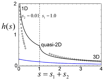
Figure 2: The behavior of $h(s)$ as the dimensionless tunneling rates of $s_{1,2}$ change independently. In the left side of the vertical dashed line, we fix $s_{2}=0.01$ and set $s_{1}=[0,1]$. In the right side, we fix $s_{1}=1$ and set $s_{2}=[0.01,3]$. The BEC behaves from 1D-like to quasi-2D like, and finally to 3D-like, as $s$ increases. The two black dotted lines denote the 1D and 3D asymptotic behaviors respectively. The blue curve describes the disorder-induced quantum depletion along the dimensional crossover, which is plotted by the functions $\frac{g^{2}_{\rm imp}n_{\rm imp}}{4\pi\tilde{g}^{2}n}\int_{-\pi}^{\pi}{\rm d}^{2}{\bm{k}}(2+s\gamma)^{-\frac{3}{2}}$ with $g^{2}_{\rm imp}n_{\rm imp}/({\tilde{g}^{2}n})=0.1$.

Equations (9) and (10) are the key results of this work. In Figs. 1 and 2, we plot $f(s)$ and $h(s)$, respectively. In the limit $s\rightarrow\infty$, the system is anisotropic 3D, whereas in the opposite limit $s\rightarrow 0$, the system is 1D. Thus, when continuously decreasing $s=2(J_{1}+J_{2})/\tilde{g}n$ by enhancing the confinement, the system necessarily crossovers from the anisotropic 3D to 1D.We emphasize that the 3D-like gas here is referred as to an optically-trapped Bose gas in the tight-binding approximation, which is different from 3D Bose gas in the almost free space. However, from the theoretical angles, we can extend the parameter regimes from tight-binding-3D-gas to beyond-tight-binding-3D-gas, i.e. entering the parameter regime of $V_{1}<5$, $V_{2}<5$. In what follows, we are surprised to find that our analytical results can recover the Lee-Huang-Yang results obtained from the 3D free space as the surprising bonus of our analytical results. To induce the hierarchical dimensional crossover, we consider the following scheme for controlling the lattice depths, which consists of two stages: (i) we first fix the lattice strength $V_{1}=5$ and increase $V_{2}$ from the initial strength of $V_{2}=5$ to the final strength of $V_{2}=12$ (i.e., $s_{2}$ is decreased to almost zero), where the system is expected to crossover from the 3D to the quasi-2D; (ii) we fix $V_{2}=12$ and further increase the value of $V_{1}$ from the initial strength of $V_{1}=5$ to the final strength of $V_{1}=12$ until the value of $s=s_{1}+s_{2}$ is almost zero.

In the process (i), the behavior of the functions of $f(s)$ and $h(s)$ are shown by the solid curves in Figs. 1 and 2. Let us first check whether our analytical results in Eqs. (9) and (10) in the limit $s\rightarrow\infty$ can recover the well-known 3D results of Bose gases. For $s\rightarrow\infty$, corresponding to the anisotropic 3D regime, we find $f(s)\simeq 1.43\sqrt{2/s}-32\sqrt{2}/(15\pi s)$ in Eq. (11) and $h(s)\simeq 8/(3\pi\sqrt{2}s)$, as denoted by the black circled curves in Figs. 1 and 2, respectively. Thus we exactly recover the 3D results of the quantum ground state energy and quantum depletion in Ref. Zhou et al. (2010). We note that our work is different from Ref. Zhou et al. (2010), where one adds a 1D optical lattice and increases the lattice depth to realize a purely 2D system. Instead, our scheme realizes the quasi-2D quantum system. To compare the two, we also plot the $f(s)$ associated with the case in Ref. Zhou et al. (2010) [see red curves in Fig. 1]. As clearly shown, our scheme realizes a quasi-2D (black curve), instead of a purely 2D, quantum system before it further crossovers to quasi-1D.

In the process (ii), we increase $V_{1}$ and fix the lattice depth $V_{2}$, where the system is expected to crossover from the quasi-2D to the quasi-1D and then to pure 1D. In particular, we note that the function $f(s)$ shown in Fig. 1 exactly approaches $3\sqrt{2}/4$ in the limit $s\rightarrow 0$, corresponding to the Lieb-Liniger result of 1D Bose gas in Ref. Orso et al. (2006). For the quantum depletion shown in Fig. 2, the function $h(s)$ diverges as $h(s)\simeq-\ln(1.35s)/\sqrt{2}$. This signals that in the absence of tunneling there is no real BEC, in agreement with the general theorems in one dimension.

Our results in Eqs. (9) and (10) complement the descriptions of dimensional crossovers described in Refs. Orso et al. (2006); Hu et al. (2009); Zhou et al. (2010); Hu and Liang (2011). We also note that the theoretical treatments beyond the Bogoliubov approximation are beyond the scope of this work.

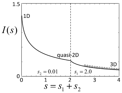
Figure 3: The behavior of $I(s)$ as the dimensionless tunneling rates of $s_{1,2}$ change independently. In the left side of the vertical dashed line, we fix $s_{2}=0.01$ and set $s_{1}=[0,2]$. In the right side, we fix $s_{1}=2$ and set $s_{2}=[0.01,2]$. The BEC behaves from 1D-like to quasi-2D like, and finally to 3D-like, as $s$ increases. The black dotted line in the right side denotes the 3D asymptotic behavior.

Superfluid density — In the second part of this paper, we apply the linear response theory to investigate the effects of disorder on the superfluid density of the BEC trapped in a 2D optical lattice. The superfluid density $\rho_{s}$ is determined by the response of the momentum density to an externally imposed velocity field. We calculate $\rho_{s}$ based on the Bogoliubov approximation. Note that Ref. Huang and Meng (1992) pioneered in the study of the superfluid density of a 3D disordered Bose gas within the framework of Bogoliubov theory, which is consistent with the results obtained by the Beliaev-Popov diagrammatic technique Lopatin and Vinokur (2002). In the context of ultracold Bose gas, one of the authors in Refs. Hu et al. (2009); Zhou et al. (2010) has investigated the disorder-induced superfluid density along the 3D-1D dimensional crossover using the Bogoliubov approximation.

In a disordered BEC, the static current-current response function consists of the low-frequency, long-wavelength longitudinal response $\chi_{L}\left(\bm{k}\right)$ and the transverse response $\chi_{T}\left(\bm{k}\right)$, i.e., $\chi_{ij}\left(\bm{k}\right)=\frac{k_{i}k_{j}}{k^{2}}\chi_{L}\left(\bm{k}\right)+(\delta_{ij}-\frac{k_{i}k_{j}}{k^{2}})\chi_{T}\left(\bm{k}\right)$, see details of the definition of $\chi_{ij}$ in Refs. Hu et al. (2009); Zhou et al. (2010). The transverse response of a BEC is only due to the normal fluid, since the superfluid component can only participate in the irrotational flow.

For the disordered BEC trapped in a 2D optical lattice described by Hamiltonian (1), where the rotational symmetry is broken, the response function along the unconfined $z$ direction is different from that in the confined $x$-$y$ plane. In the following, we assume a slow rotation with respect to the $z$ axis and calculate the transverse response function along the $z$ direction. We find

$$\rho_{n} = \lim_{k\rightarrow 0}\chi_{T}\left(\bm{k}\right)=\chi_{zz}(0,0)=\frac{2n}{m}\sum\limits_{p}\frac{p_{z}^{2}\varepsilon^{0}_{\bm{k}}}{E^{4}(\bm{k})}\langle|V_{\bm{k}}|^{2}\rangle$$ (13)

$$= \frac{\tilde{R}\sqrt{2m\tilde{g}n}}{16\hbar d^{2}}I(s),$$

where $\tilde{R}=n_{\rm imp}\tilde{b}^{2}/n\tilde{a}^{2}_{3D}$ and $I(s)$ with $s=s_{1}+s_{2}={2(J_{1}+J_{2})}/{\tilde{g}{n}}$ is given by

$$I(s)=\int_{-\pi}^{\pi}\frac{{\rm d}^{2}{\bm{k}}}{(2\pi)^{2}}\frac{2}{\sqrt{s\gamma+2}(s\gamma+1+\sqrt{s\gamma(s\gamma+2)})}.$$ (14)

Equation (13) can be interpreted as the second-order term in the perturbation expansion of the normal-fluid density in terms of the weak disorder $V_{\bm{k}}$.

The result of Eq. (13) is plotted in Fig. 3. In the asymptotic 3D limit, one finds $I(s)\simeq 4\sqrt{2}/(3\pi s)$, corresponding to the dotted curve in Fig. 3. In this case, Equation (13) recovers the corresponding result of 3D Bose gases as in Ref. Zhou et al. (2010). Equation (13) presents another key result of this paper, which provides an analytical expression for the normal fluid density in a Bose fluid in an anisotropic two-dimensional optical lattice with the presence of weak disorder. The superfluid density $\rho_{s}=\rho-\rho_{n}$ is thus straightforwardly obtained.

Discussion and conclusion — We justify the Bogoliubov approximation used in our calculations a posteriori by estimating the quantum depletion Orso et al. (2006). The experimental work Xu et al. (2006) by Ketterle’s group has shown that the Bogoliubov theory provides a semiquantitative description for an optically-trapped BEC even when the quantum depletions is in excess of $50\%$. For a uniform BEC, the quantum depletion is $(N-N_{0})/N=8/3\sqrt{na_{3D}^{2}}$ and the Bogoliubov approximation is valid provided $\sqrt{na_{3D}^{2}}$ is small. For an optically-trapped BEC, the quantum depletion is modified qualitatively as $(8m^{*}/3m)\sqrt{n\tilde{a}_{3D}/\pi}$ with $m^{*}$ being the effective mass, which remains small for typical experimental parameters as in Ref. Orso et al. (2006). For an optically-trapped Bose gas along the dimensional crossovers, we can estimate the quantum depletion $(N-N_{0})/N$ with the help of Fig. 2. Considering typical experiments in an optically-trapped BEC as in Ref. Bloch et al. (2008), the relevant parameters are: $n=3\times 10^{13}{\rm cm}^{-3}$, $d=430{\rm nm}$, $a_{3D}=5.4{\rm nm}$, and $d/\sigma_{1}\sim d/\sigma_{2}\sim 1$. The quantum depletion in Eq. (10) is thus evaluated as $(N-N_{0})/N\sim 0.0036\times h(s)$, with $h(s)$ shown in Fig. 2. It’s clear that the quantum depletion $(N-N_{0})/N<20\%$, and therefore, the Bogoliubov approximation is valid in the sprit of Ref. Xu et al. (2006). Apart from the phase fluctuations due to the tight confinement along $x$ and $y$ directions, the effect of the disorder potential can also enhance quantum fluctuations and thus affect the Bogoliubov approximation. As such, we calculate the disorder-induced correction to the quantum depletion as

$$\frac{\Delta N^{\prime}}{N}=\frac{1}{4\pi\hbar d^{2}}\sqrt{\frac{2m\tilde{g}}{n}}\frac{g^{2}_{\rm imp}n_{\rm imp}}{4\pi\tilde{g}^{2}n}\int_{-\pi}^{\pi}{\rm d}^{2}{\bm{k}}(2+s\gamma)^{-\frac{3}{2}}.$$ (15)

For the case of weak disorder of $g^{2}_{\rm imp}n_{\rm imp}/\tilde{g}^{2}n=0.1$ with $n_{\rm imp}$ being the impurity density, the quantum depletion due to the disorder along the dimensional crossover is shown by the blue curves in Fig. 2. This result indicates the quantum depletion due to the disorder is small and the Bogoliubov approximation is still valid.

Summarizing, we have investigated a 3D disordered BEC trapped in an anisotropic 2D optical lattice characterized by the lattice depths of $V_{1}$ in $x$-direction and $V_{2}$ in $y$-direction, respectively. We have derived the analytical expressions of the ground-state energy, quantum depletion and superfluid density of the system. Our results show the hierarchical, 3D-quasi-2D-1D crossovers in the behavior of quantum fluctuations and the superfluid density. The physics of the hierarchical dimensional crossover involves the interplay of three quantities: the strength of the optical lattice, the interaction between bosonic atoms, and the strength of disorder. All these quantities are experimentally controllable using state-of-the-art technologies. In particular, the depth of an optical lattice can be tuned from $0E_{R}$ to $32E_{R}$ almost at will Bloch et al. (2008). Therefore, the phenomena discussed in this paper should be observable within the current experimental capabilities. Observing this hierarchical dimensional effect directly would present an important step in revealing the interplay between dimensionality and quantum fluctuations in quasi-low dimensions. The present work is based on the Bogoliubov theory. Future studies along this direction include the treatment of the system for the whole range of interatomic interaction strength, from zero to infinity, as well as for arbitrarily strong disorder.

We thank Chao Gao for stimulating discussions. This work was supported by the Zhejiang Provincial Natural Science Foundation (Grant Nos. LZ21A040001 and LQ20A040004), the National Natural Science Foundation of China (Nos. 12074344, and 12104407) and the key projects of the Natural Science Foundation of China (Grant No. 11835011).

Note added.— Before submitting our work, we notice that a similar work Yao et al. has studied the 2D-1D dimensional crossover. In contrast, our work has focused on the gradual 3D-2D-1D dimensional crossover.

Appendix A Validity of tight-binding approximation

In the tight-binding approximation Bloch et al. (2008), the tunnelling rates of $J_{1}$ and $J_{2}$ along the $x-$ and $y-$ directions are defined as

$$J_{1}=\int_{-\infty}^{\infty}{\rm d}xw^{*}(x)\left(-\frac{\hbar^{2}}{2m}\frac{\partial^{2}}{\partial x^{2}}+V_{1}\times E_{R}\sin^{2}(q_{B}x)\right)w(x),$$ (16)

$$J_{2}=\int_{-\infty}^{\infty}{\rm d}yw^{*}(y)\left(-\frac{\hbar^{2}}{2m}\frac{\partial^{2}}{\partial y^{2}}+V_{2}\times E_{R}\sin^{2}(q_{B}y)\right)w(y),$$ (17)

with $w(x)$ and $w(y)$ being the Wannier functions in the $x-$ and $y-$ directions. The analytic solutions for the Wannier functions can be obtained by solving the 1D Mathieu problem as shown in Ref. Slater (1952). In such, the approximate analytic expressions of tunnelling rates $J_{1}$ and $J_{2}$ have been derived in Ref. Likharev and Zorin (1985)

$$\frac{J_{1}}{E_{R}}=\frac{1}{4}\left(\frac{2}{\pi}\right)^{\frac{1}{2}}\left(\frac{V_{1}}{4}\right)^{\frac{3}{4}}2^{5}\exp\left(-2\sqrt{V_{1}}\right),$$ (18)

$$\frac{J_{2}}{E_{R}}=\frac{1}{4}\left(\frac{2}{\pi}\right)^{\frac{1}{2}}\left(\frac{V_{2}}{4}\right)^{\frac{3}{4}}2^{5}\exp\left(-2\sqrt{V_{2}}\right),$$ (19)

In order for analytical expressions of $J_{1}$ and $J_{2}$ to be valid, the considered energy band must be a slowly varying function of the quasi-momentum. Hence, the potential depth s must be sufficiently large. Note that the tight-binding approximation is valid under the following conditions (i) Lattice depths od $V_{1}$ and $V_{2}$ in Eq. (2) are relatively large ($V_{1}\geq 5$, $V_{2}\geq 5$) to make sure that the interband gap of $E_{\text{gap}}$ is bigger than the chemical potential of $\mu$, i. e. $E_{\text{gap}}\gg\mu$; (ii) The overlap of the wave functions of two consecutive wells are still sufficient to ensure full coherence because of the quantum tunneling.

Now we are ready to give the rough estimations of parameter regimes of the tight-binding approximation being valid. Here, we use the typically experimental parameters of an optically-trapped Bose gas in Ref. Du et al. (2010). The typical detailed parameters read as follows: the recoil energy is $E_{R}\approx h\times 3.33{\rm kHz}$ with $h$ being Plank constant and the chemical potential of gas is $\mu\approx\tilde{g}n\approx h\times 400{\rm Hz}$. In the case of ($V_{1}\approx 5$, $V_{2}\approx 5$), we can estimate the parameters of $J_{1}/E_{R}\approx J_{2}/E_{R}\approx 0.09$ based on Eqs. (18) and (19). Then we can further estimate the dimensionless parameters used in the figures of this work as follows: $s=2(J_{1}+J_{2})/\tilde{g}n=(2(J_{1}+J_{2})/R_{R})(E_{R}/\tilde{g}n)\approx 2(0.09+0.09)\times 10=3.6$, suggesting that our model system is 3D-like. Meanwhile, as shown in Ref. Du et al. (2010), the optically-trapped Bose gas is entirely superfluid below the critical lattice height $V_{c}\approx 13E_{R}$ corresponding to $J_{1}$ and $J_{2}$ being almost zero because of the exponential decrease in Eqs. (18) and (19). We conclude that the tight-binding approximation can be regarded to be valid under $5<V_{1}<13$ and $5<V_{2}<13$, corresponding to $0<s<4$ as shown in Figs. 1 and 2.

Appendix B Detailed derivations of Eqs. (9) and (10).

In this appendix, we give the detailed derivations of Eqs. (9) and (10) . The derivation of Eq. (9) in the main text can be written as follows

$$\frac{E_{g}}{V}= \frac{\tilde{g}n^{2}}{2}+\lim\limits_{t\rightarrow 0-}\frac{1}{(2\pi)^{3}d^{2}}\int{\rm d}k_{z}{\rm d}^{2}{\bm{k}}\int\frac{{\rm d}\omega}{2\pi{\rm i}}{\rm e}^{-{\rm i}\omega t}E_{\bm{k}}G({\bm{k}},\omega)$$

$$= \frac{\tilde{g}n^{2}}{2}+\frac{1}{(2\pi)^{3}d^{2}}\int{\rm d}k_{z}{\rm d}^{2}{\bm{k}}\int_{C}\frac{{\rm d}\omega}{2\pi{\rm i}}E_{\bm{k}}G({\bm{k}},\omega),$$ (20)

with

$$\int_{C}{\rm d}\omega G(\bm{k},\omega)= \int_{C}{\rm d}\omega\frac{\omega+\varepsilon^{0}_{\bm{k}}+\tilde{g}n}{\omega^{2}-E^{2}_{\bm{k}}+{\rm i}0}$$

$$= \int_{C}{\rm d}\omega\frac{\omega+\varepsilon^{0}_{\bm{k}}+\tilde{g}n}{2E_{\bm{k}}}(\frac{1}{\omega-E_{\bm{k}}+{\rm i}0}-\frac{1}{\omega+E_{\bm{k}}-{\rm i}0})$$

$$= 2\pi{\rm i}\lim\limits_{\omega\rightarrow-E_{\bm{k}}+{\rm i}0}\frac{\omega+\varepsilon^{0}_{\bm{k}}+\tilde{g}n}{2E_{\bm{k}}}(\omega+E_{\bm{k}}-{\rm i}0)\frac{-1}{\omega+E_{\bm{k}}-{\rm i}0}$$

$$= -\pi{\rm i}\frac{\varepsilon^{0}_{\bm{k}}+\tilde{g}n-E_{\bm{k}}}{E_{\bm{k}}},$$ (21)

where we have used the residue theorem, and $C$ denotes the integration path around the upper half-plane. Then we have

$$\frac{E_{g}}{V}= \frac{\tilde{g}n^{2}}{2}-\frac{1}{(2\pi)^{3}d^{2}2}\int_{-\pi}^{\pi}{\rm d}^{2}{\bm{k}}\int_{-\infty}^{\infty}{\rm d}k_{z}(\varepsilon^{0}_{\bm{k}}+\tilde{g}n-E_{\bm{k}})$$

$$= \frac{\tilde{g}n^{2}}{2}-{\rm Int},$$ (22)

with

$${\rm Int}= \frac{1}{(2\pi)^{3}d^{2}2}\int_{-\pi}^{\pi}{\rm d}^{2}{\bm{k}}\int_{-\infty}^{\infty}{\rm d}k_{z}(\varepsilon^{0}_{\bm{k}}+\tilde{g}n-E_{\bm{k}})$$

$$= \frac{1}{(2\pi)^{3}d^{2}2}\int_{-\pi}^{\pi}{\rm d}^{2}{\bm{k}}\int_{-\infty}^{\infty}{\rm d}k_{z}(\frac{\hbar^{2}k_{z}^{2}}{2m}+2J\gamma+\tilde{g}n-\sqrt{(\frac{\hbar^{2}k_{z}^{2}}{2m}+2J\gamma)(\frac{\hbar^{2}k_{z}^{2}}{2m}+2J\gamma+2\tilde{g}n)})$$

$$= \frac{1}{(2\pi)^{3}d^{2}2\hbar}\int_{-\pi}^{\pi}{\rm d}^{2}{\bm{k}}\int_{-\infty}^{\infty}{\rm d}p_{z}(\frac{p_{z}^{2}}{2m}+2J\gamma+\tilde{g}n-\sqrt{(\frac{p_{z}^{2}}{2m}+2J\gamma)(\frac{p_{z}^{2}}{2m}+2J\gamma+2\tilde{g}n)})$$

$$= \frac{\sqrt{2m}2}{(2\pi)^{3}d^{2}2\hbar}\int_{-\pi}^{\pi}{\rm d}^{2}{\bm{k}}\int_{0}^{\infty}{\rm d}p_{z}(p_{z}^{2}+2J\gamma+\tilde{g}n-\sqrt{(p_{z}^{2}+2J\gamma)(p_{z}^{2}+2J\gamma+2\tilde{g}n)})$$

$$= \frac{\sqrt{2m}\tilde{g}n\sqrt{\tilde{g}n}}{(2\pi)^{3}d^{2}\hbar}\int_{-\pi}^{\pi}{\rm d}^{2}{\bm{k}}\int_{0}^{\infty}{\rm d}p_{z}(p_{z}^{2}+s\gamma+1-\sqrt{(p_{z}^{2}+s\gamma)(p_{z}^{2}+s\gamma+2)}),$$ (23)

where $\gamma=1-\frac{J_{1}}{J}\cos(k_{x})-\frac{J_{2}}{J}\cos(k_{y})$ and $s=\frac{2J}{\tilde{g}n}$. We then let $p_{z}^{2}+s\gamma=\beta$,

$${\rm Int}=\frac{\sqrt{2m}\tilde{g}n\sqrt{\tilde{g}n}}{(2\pi)^{3}d^{2}\hbar}\int_{-\pi}^{\pi}{\rm d}^{2}{\bm{k}}\int_{s\gamma}^{\infty}\frac{{\rm d}\beta}{2\sqrt{\beta-s\gamma}}(\beta+1-\sqrt{\beta(\beta+2)}).$$ (24)

We then let $s\gamma/\beta=\tau$, and ${\rm d}\beta=-s\gamma{\rm d}\tau/\tau^{2}$,

$${\rm Int}= \frac{\sqrt{2m}\tilde{g}n\sqrt{\tilde{g}n}}{(2\pi)^{3}d^{2}\hbar 2}\int_{-\pi}^{\pi}{\rm d}^{2}{\bm{k}}\int_{0}^{1}\frac{s\gamma}{\tau^{2}}{\rm d}\tau\frac{1}{\sqrt{\frac{s\gamma}{\tau}-s\gamma}}(\frac{s\gamma}{\tau}+1-\sqrt{\frac{s\gamma}{\tau}(\frac{s\gamma}{\tau}+2)})$$

$$= \frac{\sqrt{2m}\tilde{g}n\sqrt{\tilde{g}n}}{(2\pi)^{3}d^{2}\hbar 2}\int_{-\pi}^{\pi}{\rm d}^{2}{\bm{k}}\int_{0}^{1}{\rm d}\tau\frac{\sqrt{s\gamma}}{\sqrt{\tau}}\frac{1}{\sqrt{1-\tau}}(\frac{s\gamma}{\tau^{2}}+\frac{1}{\tau}-\frac{s\gamma}{\tau^{2}}\sqrt{1+\frac{2\tau}{s\gamma}})$$

$$= \frac{\sqrt{2m}\tilde{g}n\sqrt{\tilde{g}n}}{(2\pi)^{3}d^{2}\hbar 2}\int_{-\pi}^{\pi}{\rm d}^{2}{\bm{k}}\frac{1}{\sqrt{s\gamma}}\int_{0}^{1}{\rm d}\tau\frac{1}{\sqrt{\tau}}\frac{1}{\sqrt{1-\tau}}(\frac{(s\gamma)^{2}}{\tau^{2}}+\frac{s\gamma}{\tau}-\frac{(s\gamma)^{2}}{\tau^{2}}\sqrt{1+\frac{2\tau}{s\gamma}}),$$ (25)

where the integration about $\tau$ can be written as the hypergeometric function

$$\int_{0}^{1}{\rm d}\tau\frac{1}{\sqrt{\tau}}\frac{1}{\sqrt{1-\tau}}(\frac{(s\gamma)^{2}}{\tau^{2}}+\frac{s\gamma}{\tau}-\frac{(s\gamma)^{2}}{\tau^{2}}\sqrt{1+\frac{2\tau}{s\gamma}})=\frac{\pi}{2}{}_{2}F_{1}[\frac{1}{2},\frac{3}{2},3,\frac{-2}{s\gamma}],$$ (26)

hence we obtain

$${\rm Int}= \frac{\sqrt{2m}\tilde{g}n\sqrt{\tilde{g}n}}{(2\pi)^{3}d^{2}\hbar 2}\int_{-\pi}^{\pi}{\rm d}^{2}{\bm{k}}\frac{1}{\sqrt{s\gamma}}\frac{\pi}{2}{}_{2}F_{1}[\frac{1}{2},\frac{3}{2},3,\frac{-2}{s\gamma}]$$

$$= \frac{\sqrt{2m\tilde{g}n}\tilde{g}n}{4\pi\hbar d^{2}}\frac{\pi}{2}\int_{-\pi}^{\pi}\frac{{\rm d}^{2}{\bm{k}}}{(2\pi)^{2}}\frac{1}{\sqrt{s\gamma}}{}_{2}F_{1}[\frac{1}{2},\frac{3}{2},3,\frac{-2}{s\gamma}]$$

$$= \frac{\sqrt{2m\tilde{g}n}\tilde{g}n}{4\pi\hbar d^{2}}f(s),$$ (27)

with

$$f(s)=\frac{\pi}{2}\int_{-\pi}^{\pi}\frac{{\rm d}^{2}{\bm{k}}}{(2\pi)^{2}}\frac{1}{\sqrt{s\gamma}}{}_{2}F_{1}[\frac{1}{2},\frac{3}{2},3,\frac{-2}{s\gamma}].$$ (28)

Finally we get the Eqs. (9) in the main text

$$\frac{E_{g}}{V}= \frac{\tilde{g}n^{2}}{2}-{\rm Int}$$

$$= \frac{\tilde{g}n^{2}}{2}-\frac{\sqrt{2m\tilde{g}n}\tilde{g}n}{4\pi\hbar d^{2}}f(s).$$ (29)

The derivation of Eqs. (10) in the main text is as follows

$$\frac{N-N_{0}}{N}= \lim\limits_{t\rightarrow 0-}\frac{{\rm i}}{(2\pi)^{4}d^{2}n}\int{\rm d}k_{z}{\rm d}^{2}{\bm{k}}\int{\rm d}\omega{\rm e}^{-{\rm i}\omega t}G(\bm{k},\omega)$$

$$= \frac{{\rm i}}{(2\pi)^{4}d^{2}n}\int{\rm d}k_{z}{\rm d}^{2}{\bm{k}}\int_{C}{\rm d}\omega G(\bm{k},\omega)$$

$$= \frac{{\rm i}}{(2\pi)^{4}d^{2}n}\int{\rm d}k_{z}{\rm d}^{2}{\bm{k}}(-\pi{\rm i})\frac{\varepsilon^{0}_{\bm{k}}+\tilde{g}n-E_{\bm{k}}}{E_{\bm{k}}}$$

$$= \frac{1}{2(2\pi)^{3}d^{2}n}\int{\rm d}k_{z}{\rm d}^{2}{\bm{k}}\frac{\varepsilon^{0}_{\bm{k}}+\tilde{g}n-E_{\bm{k}}}{E_{\bm{k}}}$$

$$= \frac{1}{2(2\pi)^{3}d^{2}n}\int_{-\pi}^{\pi}{\rm d}^{2}{\bm{k}}\int_{-\infty}^{\infty}{\rm d}k_{z}[\frac{\frac{\hbar^{2}k_{z}^{2}}{2m}+2J\gamma+\tilde{g}n}{\sqrt{(\frac{\hbar^{2}k_{z}^{2}}{2m}+2J\gamma)(\frac{\hbar^{2}k_{z}^{2}}{2m}+2J\gamma+2\tilde{g}n)}}-1]$$

$$= \frac{1}{2(2\pi)^{3}\hbar d^{2}n}\int_{-\pi}^{\pi}{\rm d}^{2}{\bm{k}}\int_{-\infty}^{\infty}{\rm d}p_{z}[\frac{\frac{p_{z}^{2}}{2m}+2J\gamma+\tilde{g}n}{\sqrt{(\frac{p_{z}^{2}}{2m}+2J\gamma)(\frac{p_{z}^{2}}{2m}+2J\gamma+2\tilde{g}n)}}-1]$$

$$= \frac{\sqrt{2m}}{2(2\pi)^{3}\hbar d^{2}n}\int_{-\pi}^{\pi}{\rm d}^{2}{\bm{k}}\int_{-\infty}^{\infty}{\rm d}p_{z}[\frac{p_{z}^{2}+2J\gamma+\tilde{g}n}{\sqrt{(p_{z}^{2}+2J\gamma)(p_{z}^{2}+2J\gamma+2\tilde{g}n)}}-1]$$

$$= \frac{\sqrt{2m}}{2(2\pi)^{3}\hbar d^{2}n}\int_{-\pi}^{\pi}{\rm d}^{2}{\bm{k}}2\int_{0}^{\infty}\frac{{\rm d}\eta}{2\sqrt{\eta}}[\frac{\eta+2J\gamma+\tilde{g}n}{\sqrt{(\eta+2J\gamma)(\eta+2J\gamma+2\tilde{g}n)}}-1]$$

$$= \frac{\sqrt{2m\tilde{g}n}}{2(2\pi)^{3}\hbar d^{2}n}\int_{-\pi}^{\pi}{\rm d}^{2}{\bm{k}}\int_{0}^{\infty}\frac{{\rm d}\eta}{\sqrt{\eta}}[\frac{\eta+s\gamma+1}{\sqrt{(\eta+s\gamma)(\eta+s\gamma+2)}}-1]$$

$$= \frac{1}{4\pi\hbar d^{2}}\sqrt{\frac{2m\tilde{g}}{n}}\int_{-\pi}^{\pi}\frac{{\rm d}^{2}{\bm{k}}}{(2\pi)^{2}}\int_{0}^{\infty}\frac{{\rm d}\eta}{\sqrt{\eta}}[\frac{\eta+s\gamma+1}{\sqrt{(\eta+s\gamma)(\eta+s\gamma+2)}}-1]$$

$$= \frac{1}{4\pi\hbar d^{2}}\sqrt{\frac{2m\tilde{g}}{n}}h(s),$$ (30)

with

$$h(s)=\int_{-\pi}^{\pi}\frac{{\rm d}^{2}{\bm{k}}}{(2\pi)^{2}}\int_{0}^{\infty}\frac{{\rm d}\eta}{\sqrt{\eta}}[\frac{\eta+s\gamma+1}{\sqrt{(\eta+s\gamma)(\eta+s\gamma+2)}}-1].$$ (31)

References

Lee et al. (2006)Patrick A. Lee, Naoto Nagaosa, and Xiao-Gang Wen, “Doping a mott
insulator: Physics of high-temperature superconductivity,” Rev.
Mod. Phys. 78, 17–85
(2006).
Cao et al. (2018a)Yuan Cao, Valla Fatemi,
Ahmet Demir, Shiang Fang, Spencer L. Tomarken, Jason Y. Luo, Javier D. Sanchez-Yamagishi, Kenji Watanabe, Takashi Taniguchi, Efthimios Kaxiras, Ray C. Ashoori, and Pablo Jarillo-Herrero, “Correlated insulator behaviour at half-filling
in magic-angle graphene superlattices,” Nature 556, 80–84 (2018a).
Cao et al. (2018b)Yuan Cao, Valla Fatemi,
Ahmet Demir, Shiang Fang, Spencer L. Tomarken, Jason Y. Luo, Javier D. Sanchez-Yamagishi, Kenji Watanabe, Takashi Taniguchi, Efthimios Kaxiras, Ray C. Ashoori, and Pablo Jarillo-Herrero, “Correlated insulator behaviour at half-filling
in magic-angle graphene superlattices,” Nature 556, 80–84 (2018b).
Tarnopolsky et al. (2019)Grigory Tarnopolsky, Alex Jura Kruchkov, and Ashvin Vishwanath, “Origin of
magic angles in twisted bilayer graphene,” Phys. Rev. Lett. 122, 106405 (2019).
Haldane (1981)F. D. M. Haldane, “Effective harmonic-fluid approach to low-energy properties of
one-dimensional quantum fluids,” Phys. Rev. Lett. 47, 1840–1843 (1981).
Bloch et al. (2008)Immanuel Bloch, Jean Dalibard, and Wilhelm Zwerger, “Many-body
physics with ultracold gases,” Rev. Mod. Phys. 80, 885–964 (2008).
Paredes et al. (2004)Belén Paredes, Artur Widera, Valentin Murg, Olaf Mandel, Simon Fölling, Ignacio Cirac, Gora V. Shlyapnikov, Theodor W. Hänsch, and Immanuel Bloch, “Tonks–girardeau gas of ultracold atoms in an optical lattice,” Nature 429, 277–281
(2004).
Peppler et al. (2018)T. Peppler, P. Dyke,
M. Zamorano, I. Herrera, S. Hoinka, and C. J. Vale, “Quantum anomaly and 2d-3d crossover in strongly
interacting fermi gases,” Phys. Rev. Lett. 121, 120402 (2018).
Holten et al. (2018)M. Holten, L. Bayha,
A. C. Klein, P. A. Murthy, P. M. Preiss, and S. Jochim, “Anomalous breaking of scale invariance in a
two-dimensional fermi gas,” Phys. Rev. Lett. 121, 120401 (2018).
Orso et al. (2006)G. Orso, C. Menotti, and S. Stringari, “Quantum fluctuations and
collective oscillations of a bose-einstein condensate in a 2d optical
lattice,” Phys. Rev. Lett. 97, 190408 (2006).
Hu et al. (2009)Ying Hu, Zhaoxin Liang, and Bambi Hu, “Effects of disorder on
quantum fluctuations and superfluid density of a bose-einstein condensate in
a two-dimensional optical lattice,” Phys.
Rev. A 80, 043629
(2009).
Hu and Liang (2011)Ying Hu and Zhaoxin Liang, “Visualization of
dimensional effects in collective excitations of optically trapped
quasi-two-dimensional bose gases,” Phys. Rev. Lett. 107, 110401 (2011).
Zhou et al. (2010)Kezhao Zhou, Ying Hu,
Zhaoxin Liang, and Zhidong Zhang, “Optically trapped
quasi-two-dimensional bose gases in a random environment: Quantum
fluctuations and superfluid density,” Phys.
Rev. A 82, 043609
(2010).
Faigle-Cedzich et al. (2021)Bruno M. Faigle-Cedzich, Jan M. Pawlowski, and Christof Wetterich, “Dimensional crossover in ultracold fermi gases from
functional renormalization,” Phys. Rev. A 103, 033320 (2021).
Hu et al. (2019)Hui Hu, Brendan C. Mulkerin, Umberto Toniolo, Lianyi He, and Xia-Ji Liu, “Reduced quantum anomaly in a
quasi-two-dimensional fermi superfluid: Significance of the
confinement-induced effective range of interactions,” Phys. Rev. Lett. 122, 070401 (2019).
Yin et al. (2020)X. Y. Yin, Hui Hu, and Xia-Ji Liu, “Few-body perspective of a quantum
anomaly in two-dimensional fermi gases,” Phys. Rev. Lett. 124, 013401 (2020).
(17)Hepeng Yao, Lorenzo Pizzino,
and Thierry Giamarchi, “Strongly-interacting bosons at 2d-1d dimensional crossover,” arXiv:2204.02240v1 .
White et al. (2009) M. White, M. Pasienski, D. McKay, S. Q. Zhou, D. Ceperley, and B. DeMarco, “Strongly
interacting bosons in a disordered optical lattice,” Phys. Rev. Lett. 102, 055301 (2009).
Paiva et al. (2015)Thereza Paiva, Ehsan Khatami,
Shuxiang Yang, Valéry Rousseau, Mark Jarrell, Juana Moreno, Randall G. Hulet, and Richard T. Scalettar, “Cooling atomic gases with disorder,” Phys. Rev. Lett. 115, 240402 (2015).
Petrov et al. (2000)D. S. Petrov, M. Holzmann, and G. V. Shlyapnikov, “Bose-einstein condensation
in quasi-2d trapped gases,” Phys. Rev. Lett. 84, 2551–2555 (2000).
Huang and Meng (1992)Kerson Huang and Hsin-Fei Meng, “Hard-sphere bose
gas in random external potentials,” Phys.
Rev. Lett. 69, 644–647
(1992).
Astrakharchik et al. (2002)G. E. Astrakharchik, J. Boronat, J. Casulleras,
and S. Giorgini, “Superfluidity versus
bose-einstein condensation in a bose gas with disorder,” Phys.
Rev. A 66, 023603
(2002).
Yao et al. (2020)Hepeng Yao, Thierry Giamarchi, and Laurent Sanchez-Palencia, “Lieb-liniger bosons in a shallow quasiperiodic potential: Bose glass phase
and fractal mott lobes,” Phys. Rev. Lett. 125, 060401 (2020).
Peng et al. (2010)Shi-Guo Peng, Seyyed S. Bohloul, Xia-Ji Liu,
Hui Hu, and Peter D. Drummond, “Confinement-induced resonance in
quasi-one-dimensional systems under transversely anisotropic confinement,” Phys. Rev. A 82, 063633 (2010).
Zhang and Zhang (2011)Wei Zhang and Peng Zhang, “Confinement-induced resonances in quasi-one-dimensional traps with
transverse anisotropy,” Phys. Rev. A 83, 053615 (2011).
Bergeman et al. (2003)T. Bergeman, M. G. Moore,
and M. Olshanii, “Atom-atom scattering under
cylindrical harmonic confinement: Numerical and analytic studies of the
confinement induced resonance,” Phys. Rev. Lett. 91, 163201 (2003).
Souza et al. (2021)R S Souza, Axel Pelster, and F E A dos Santos, “Green’s function approach to
the bose–hubbard model with disorder,” New
Journal of Physics 23, 083007 (2021).
Lopatin and Vinokur (2002)A. V. Lopatin and V. M. Vinokur, “Thermodynamics
of the superfluid dilute bose gas with disorder,” Phys. Rev. Lett. 88, 235503 (2002).
Xu et al. (2006)K. Xu, Y. Liu, D. E. Miller, J. K. Chin, W. Setiawan, and W. Ketterle, “Observation of strong quantum depletion in a gaseous
bose-einstein condensate,” Phys. Rev. Lett. 96, 180405 (2006).
Likharev and Zorin (1985)K. K. Likharev and A .B. Zorin, “Theory of the
bloch-wave oscillations in small josephson junctions,” J. Low. Temp.
Phys. 59, 347 (1985).
Du et al. (2010)X Du,
Shoupu Wan, Emek Yesilada, C Ryu, D J Heinzen, Zhaoxin Liang, and Biao Wu, “Bragg
spectroscopy of a superfluid bose–hubbard gas,” New Journal of Physics 12, 083025 (2010).