Explosive behaviour in networks of Winfree oscillators

Abstract.

We consider directed networks of Winfree oscillators with power law distributed in- and out-degree distributions. Gaussian and power law distributed intrinsic frequencies are considered, and these frequencies are positively correlated with oscillators’ in-degrees. The Ott/Antonsen ansatz is used to derive degree-based mean field equations for the expected dynamics of networks, and these are numerically analysed. In a variety of cases “explosive” transitions between either two different steady states or between a steady state and a periodic solution are found, and these transitions are explained using bifurcation theory.

1. Introduction

The study of networks is driven by the many real-world systems which can be represented in this way [23], such as networks of neuronal [28], cardiac [4] or smooth muscle [40] cells. In networks of oscillators it is often the conditions under which the oscillators synchronise which are of interest [29, 36]. For networks of nonidentical oscillators there is often a continuous transition from asynchrony to higher and higher levels of synchrony as the strength of coupling between oscillators is increased [12, 36]. But recently a different form of transition known as “explosive synchrony” (ES) has been observed. Here, there is a discontinuous increase in network coherence as the coupling strength between oscillators is increased (see [6] for a review). This behaviour was first reported by [8] in an undirected network of Kuramoto oscillators [12] for which the intrinsic frequency of an oscillator was equal to its degree, the degrees having an inverse power law distribution. The authors emphasised that the explosive transition was due to there being a relationship between a local network property (an oscillator’s degree) and a property of an oscillator (its intrinsic frequency) — in this case a positive correlation between the two. Since the publication of [8] there have been many studies of ES [17, 2, 42, 41].

As recently noted by [11], ES is not actually an unexpected phenomenon, since if there is a continuous transition to synchrony through either a transcritical or pitchfork bifurcation as, say, the strength of coupling between oscillators is increased, then by varying a second parameter sufficiently the criticality of the bifurcation will change. This change leads to bistability and a region of hysteresis as the original parameter is varied (i.e. an “explosive” transition).

Many studies of ES use Kuramoto phase oscillators which are coupled through phase differences. However, more realistic oscillators are not coupled in this way, instead having interactions which depend on the states of the two oscillators which are coupled [37, 21, 3, 19]. The oscillator we study – the Winfree model [39] – is a phase oscillator similar in form to the Kuramoto oscillator but is not described with phase differences, instead involving a “phase response curve” and a pulsatile function of phase. We are not aware of any reports of ES in networks of Winfree oscillators, and as one of our contributions we report here our observations of this phenomenon in our numerical explorations of networks of Winfree oscillators in a variety of network configurations.

Most previous studies of networks of Winfree oscillators have focused on the all-to-all coupled case [1, 26, 10, 7, 27], with an exception being [16]. Many previous studies of ES have considered undirected networks, where oscillators are either coupled or not. However, we consider directed networks – as seen in neuronal systems – where one oscillator influences other oscillators coupled downstream but without necessarily a reciprocal influence back upstream.

The bistability that often accompanies ES is of interest as it allows a network to have more than one stable state for a given set of parameters, with the current state often determined by the network’s history. A prominent example of such bistability is in networks which exhibit Up and Down states [38, 30], with transitions between these states driven by either fluctuations or noise of some form, or by transient inputs. The abrupt transitions between states may also provide a model for the conscious-unconscious transition when awaking from anesthesia [35].

The structure of the paper is as follows. In Sec. 2 we present the network we consider and the degree-based mean field description of its dynamics, derived using the Ott/Antonsen ansatz. Specific cases of independent in- and out-degrees, and equal in- and out-degrees, are considered. In Sec. 3 we consider a Gaussian distribution of intrinsic frequencies which are positively correlated with oscillators’ in-degrees. In Sec. 4 we consider an inverse power law distribution of intrinsic frequencies and again correlate them with oscillators’ in-degrees. We consider the cases of independent in- and out-degrees, and equal in- and out-degrees. A variety of “explosive” transitions are observed and explained using simple bifurcation theory. We conclude in Sec. 5.

2. Model

The model describing a directed network of Winfree oscillators is as presented in [16, 26]:

$$\frac{d\theta_{j}}{dt}=\omega_{j}+U(\theta_{j})\frac{\epsilon}{\langle k\rangle}\sum_{n=1}^{N}A_{jn}T(\theta_{n});\qquad j=1,2\dots N$$ (1)

where $\epsilon$ is the strength of coupling, $\langle k\rangle$ is the mean degree of the network and the connectivity is given by the adjacency matrix $A$ with $A_{jn}=1$ if oscillator $n$ connects to oscillator $j$ and zero otherwise. The $\omega_{j}$ are chosen from a Lorentzian distribution with centre and half-width at half-maximum to be discussed below. The phase response curve [32, 22] is chosen to be $U(\theta)=-\sin{\theta}$ and the pulsatile function $T$ which has a maximum at $\theta=0$ is

$$T(\theta)=\frac{8}{35}(1+\cos{\theta})^{4}$$ (2)

The in-degree of oscillator $j$ is

$$k_{in,j}=\sum_{n=1}^{N}A_{jn}$$ (3)

and the out-degree of oscillator $n$ is

$$k_{out,n}=\sum_{j=1}^{N}A_{jn}$$ (4)

We consider large networks where all in- and out-degrees are large and assume that the network can be characterised by its degree distribution $P({\bf k})$ where ${\bf k}=(k_{in},k_{out})$, and an assortativity function $a({\bf k}^{\prime}\to{\bf k})$ giving the probability that an oscillator with degree ${\bf k}^{\prime}$ connects to one with degree ${\bf k}$, given that such oscillators exist. $P({\bf k})$ is normalised such that $\sum_{{\bf k}}P({\bf k})=N$ and we choose the marginal distributions of the in-degrees and the out-degrees to be equal.

Using the theory in [16] (or see [15, 5] for similar derivations) one can show that the long-time dynamics of the network is described by

$$\frac{\partial b({\bf k},t)}{\partial t}=\frac{\epsilon R({\bf k},t)}{2}+[i\omega_{0}({\bf k})-\Delta({\bf k})]b({\bf k},t)-\frac{\epsilon R({\bf k},t)}{2}[b({\bf k},t)]^{2}$$ (5)

where $\omega_{0}({\bf k})$ and $\Delta({\bf k})$ are the centre and half-width at half-maximum, respectively, of the Lorentzian distribution from which the values of $\omega_{j}$ for oscillators with degree ${\bf k}$ are chosen:

$$g(\omega({\bf k}))=\frac{\Delta({\bf k})/\pi}{[\omega({\bf k})-\omega_{0}({\bf k})]^{2}+\Delta^{2}({\bf k})}$$ (6)

The variable

$$b({\bf k},t)=\int_{-\infty}^{\infty}\int_{0}^{2\pi}f(\theta,\omega|{\bf k},t)e^{-i\theta}d\theta\ d\omega$$ (7)

is the complex-valued order parameter for oscillators with degree ${\bf k}$, where $f(\theta,\omega|{\bf k},t)d\theta d\omega$ is the probability that an oscillator with degree ${\bf k}$ has phase in $[\theta,\theta+d\theta]$ and frequency in $[\omega,\omega+d\omega]$ at time $t$. $R({\bf k},t)$ is given by

$$R({\bf k},t)=\frac{1}{\langle k\rangle}\sum_{{\bf k}^{\prime}}P({\bf k}^{\prime})a({\bf k}^{\prime}\to{\bf k})G({\bf k}^{\prime},t)$$ (8)

where

$$G({\bf k},t) = 1+\frac{4\left[b({\bf k},t)+\overline{b}({\bf k},t)\right]}{5}+\frac{2\left[b^{2}({\bf k},t)+\overline{b}^{2}({\bf k},t)\right]}{5}$$ (9)

$$+\frac{4\left[b^{3}({\bf k},t)+\overline{b}^{3}({\bf k},t)\right]}{35}+\frac{b^{4}({\bf k},t)+\overline{b}^{4}({\bf k},t)}{70}$$

where overline indicates the complex conjugate. The form of $G$ is determined by the function $T(\theta)$. This derivation of a degree-dependent mean field description uses the Ott/Antonsen ansatz [24, 25]. A crucial ingredient for the use of this ansatz is the sinusoidal form of the function $U(\theta)$.

We are interested in the case of neutral assortativity, for which [31]

$$a({\bf k}^{\prime}\to{\bf k})=\frac{k_{out}^{\prime}k_{in}}{N\langle k\rangle}$$ (10)

and cases where either the in- and out-degree of an oscillator are independent, or they are equal (and thus perfectly correlated). Writing $P(k_{in}^{\prime},k_{out}^{\prime})$ instead of $P({\bf k}^{\prime})/N$ we have

$$R(k_{in},k_{out})=\frac{k_{in}}{\langle k\rangle^{2}}\sum_{k_{in}^{\prime}}\sum_{k_{out}^{\prime}}P(k_{in}^{\prime},k_{out}^{\prime})k_{out}^{\prime}G(k_{in}^{\prime},k_{out}^{\prime},t)$$ (11)

which is clearly independent of $k_{out}$. Thus both $b$ and $G$ must also be independent of $k_{out}$ and we have

$$R(k_{in},t)=\frac{k_{in}}{\langle k\rangle^{2}}\sum_{k_{in}^{\prime}}Q(k_{in}^{\prime})G(k_{in}^{\prime},t)$$ (12)

where

$$Q(k_{in}^{\prime})=\sum_{k_{out}^{\prime}}P(k_{in}^{\prime},k_{out}^{\prime})k_{out}^{\prime}.$$ (13)

For the case of the in- and out-degrees of an oscillator being independent, $P(k_{in}^{\prime},k_{out}^{\prime})$ factorises: $P(k_{in}^{\prime},k_{out}^{\prime})=p(k_{in})p(k_{out}^{\prime})$ where $p$ is the marginal distribution of either the in- or out-degrees. In this case,

$$R(k_{in},t)=\frac{k_{in}}{\langle k\rangle}\sum_{k_{in}^{\prime}}p(k_{in}^{\prime})G(k_{in}^{\prime},t).$$ (14)

Alternatively, if $k_{in}=k_{out}$ for each oscillator (i.e. each oscillator has the same in- and out-degree) then $Q(k_{in}^{\prime})=k_{in}^{\prime}p(k_{in}^{\prime})$ and

$$R(k_{in},t)=\frac{k_{in}}{\langle k\rangle^{2}}\sum_{k_{in}^{\prime}}p(k_{in}^{\prime})k_{in}^{\prime}G(k_{in}^{\prime},t).$$ (15)

In either case the “input” to an oscillator with in-degree $k_{in}$ is proportional to its in-degree, i.e. $k_{in}$.

One could use this theory to investigate the effects of choosing different degree distributions $p$ as in [14] but instead we fix $p$ as a power law distribution and look at the effects of correlating an oscillator’s frequency with its degree. Specifically, we make $\Delta$ independent of degree but choose $\omega_{0}$ to be a function of $k_{in}$ only. (One could make $\omega_{0}$ a function of $k_{out}$ as well, or instead, but doing so increases the computational cost, and the phenomena we are interested in occur when $\omega_{0}$ is a function of $k_{in}$ only.) Thus the equations of interest are

$$\frac{\partial b(k_{in},t)}{\partial t}=\frac{\epsilon R(k_{in},t)}{2}+[i\omega_{0}(k_{in})-\Delta]b(k_{in},t)-\frac{\epsilon R(k_{in},t)}{2}[b(k_{in},t)]^{2}$$ (16)

where $m\leq k_{in}\leq M$, where $m$ and $M$ are the minimum and maximum in- and out-degrees respectively, $R$ is given by either (14) or (15) and $G$ is given by (9) but with only dependence on in-degree.

Note that in previous work [16] we used similar equations as those above to investigate the effects of varying the correlation between in- and out-degrees of Winfree oscillators, and of parameter- and degree-based assortativity. We also examined the effects of correlating oscillators’ intrinsic frequencies with their in-degrees, but did not consider varying the coupling strength. Also, there we considered uniform degree distributions rather than power law, as we do here and as many other researchers do.

Below we will use the mean firing frequency of a network to describe its behaviour, so now derive an expression for that. The dynamics of an oscillator with in-degree $k_{in}$ is

$$\frac{d\theta}{dt}=\omega(k_{in})-\epsilon R(k_{in})\sin{\theta}.$$ (17)

If $|\omega(k_{in})|>\epsilon R(k_{in})$ then the oscillator will fire periodically with frequency

$$\frac{\sqrt{\omega^{2}(k_{in})-\epsilon^{2}R^{2}(k_{in})}}{2\pi}.$$ (18)

Thus the expected frequency for oscillators with in-degree $k_{in}$ is

$$f(k_{in}) =\frac{1}{2\pi}\mbox{Re}\left(\int_{-\infty}^{\infty}g(\omega(k_{in}))\sqrt{\omega^{2}(k_{in})-\epsilon^{2}R^{2}(k_{in})}\ d\omega(k_{in})\right)$$

$$=\frac{1}{2\pi}\sqrt{\frac{\omega_{0}^{2}(k_{in})-\Delta^{2}-\epsilon^{2}R^{2}(k_{in})+\sqrt{[\omega_{0}^{2}(k_{in})-\Delta^{2}-\epsilon^{2}R^{2}(k_{in})]^{2}+4\Delta^{2}\omega_{0}^{2}(k_{in})}}{2}}$$ (19)

where $g$ is the Lorentzian (6) and thus the mean firing rate over the network is

$$F=\frac{1}{2\pi}\sum_{k_{in}}p(k_{in})f(k_{in})$$ (20)

For comparison with our results below we briefly describe the dynamics of a fully connected network of Winfree oscillators. Two types of behaviour are typically seen in such a network: synchronous and asynchronous [26, 7], although the fraction of oscillators actually oscillating varies in different asynchronous states. Increasing $\epsilon$ tends to destroy synchronous behaviour through a saddle-node-on-invariant-circle (SNIC) bifurcation, as many of the oscillators “lock” to an approximate fixed point. For moderate $\epsilon$ increasing the spread of intrinsic frequencies tends to destroy synchronous behaviour through a supercritical Hopf bifurcation, as the oscillators become too dissimilar in frequency to synchronise [26]. Below we will see a wider variety of bifurcations resulting from the networks’ structure.

3. Gaussian frequency distribution

We choose the degree distribution $p(k)$ to be a truncated power law distribution with exponent $-3$, as many others have done when studying ES [18, 8]:

$$p(k)=\begin{cases}a/k^{3}&m\leq k\leq M\\ 0&\mbox{ otherwise}\end{cases}$$ (21)

where $a$ is a normalisation such that

$$\sum_{k=m}^{M}\frac{a}{k^{3}}=1.$$ (22)

Since the degrees are all large (i.e. $1\ll m$) we treat $k$ as a continuous variable and approximate the sum in (22) by an integral, giving $a=2m^{2}M^{2}/(M^{2}-m^{2})$. The cumulative distribution function for $k$ is

$$\widehat{p}(k)=\int_{m}^{k}p(s)\ ds=\frac{a}{2}\left(\frac{1}{m^{2}}-\frac{1}{k^{2}}\right).$$ (23)

We need to specify the dependence of $\omega_{0}$ on $k_{in}$. In this section we consider the case where for a particular realisation of the network, we randomly choose the target frequencies from a Gaussian distribution with mean 1 and standard deviation $\sigma$, then assign the smallest target frequency to the oscillator with smallest in-degree, the second smallest target frequency to the oscillator with second smallest in-degree, etc. (For oscillators with equal in-degree, they are ranked in random order.) For oscillator $j$ the actual $\omega_{j}$ is then chosen from a Lorentzian with centre equal to the target frequency for oscillator $j$ and half-width at half-maximum (HWHM) equal to $\Delta$, similar to the scheme in [34].

In this case we have

$$\omega_{0}(k)=\widehat{q}^{-1}(\widehat{p}(k))$$ (24)

where $\widehat{q}$ is the cumulative distribution function of the appropriate Gaussian distribution, i.e.

$$\widehat{q}(\omega)=\frac{1}{2}\left[1+\mbox{erf}\left(\frac{\omega-1}{\sqrt{2}\sigma}\right)\right]$$ (25)

A demonstration of this is shown in Fig. 1 where we create a directed network with $N=2000$ nodes using the configuration model [23], then randomly chose $N$ target frequencies from a Gaussian distribution with mean 1 and standard deviation $0.01$, then associated the smallest frequency with the node with smallest in-degree etc. These values are shown as dots in panel (a), along with the theoretical relationship (24). Panel (b) shows the actual values of the $\omega_{j}$ (dots), taken from a Lorentzian with centre equal to the values in panel (a) and HWHM 0.00005.

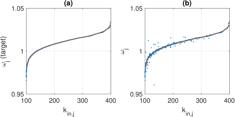
Figure 1. (a): solid line: (24); dots: target frequencies and degrees for one realisation of a network. (b): solid line: (24); dots: actual frequencies and degrees for one realisation of a network. Parameters: $m=100,M=400,N=2000,\sigma=0.01,\Delta=0.00005$.

Clearly there is a positive correlation between $k_{in,j}$ and $\omega_{j}$, but the Pearson correlation coefficient between them, defined by

$$\rho_{k\omega}=\frac{\sum_{j=1}^{N}(k_{in,j}-\langle k\rangle)(\omega_{j}-\bar{\omega})}{\sqrt{\sum_{j=1}^{N}(k_{in,j}-\langle k\rangle)^{2}}\sqrt{\sum_{j=1}^{N}(\omega_{j}-\bar{\omega})^{2}}}$$ (26)

where $\bar{\omega}$ is the mean of the $\omega_{j}$, is less than 1 and (using this construction) cannot be systematically varied, as was possible in [16, 15]. Note that the idea of not having a perfect match between an oscillator’s degree and a prescribed frequency (as we have here for $\Delta\neq 0$) was discussed in [33], where it was shown that such a mismatch actually created ES.

To investigate the influence of varying the correlation between $k_{in,j}$ and $\omega_{j}$, we created a sequence of the appropriate degrees, chose values of $\omega$ from a Gaussian distribution and randomly paired them. We then repeatedly performed Monte Carlo swaps of $\omega$ values; potential swaps were accepted if they increased the Pearson correlation coefficient toward a target value – typically a positive number. This approach required substantial effort to satisfy high correlations $(\geq 0.9)$, since a sequence of $\omega$ randomly paired with degree sequences typically exhibited no correlation. Alternatively, we maximised the correlation between the $k_{in,j}$ and $\omega_{j}$ by initially sorting both sequences as above. Aligning maximal-minimal values then produced the highest possible correlation coefficient for given sequences which we then reduced using Monte Carlo swaps, with swaps accepted if they pushed the correlation value toward a target value. Sequences of degrees and frequencies generated with this approach were assembled into adjacency matrices utilising our network assembly scheme, the “permutation method”, presented previously [20]. Note that with this approach of constructing networks the Ott/Antonsen approach cannot be used, and we must simulate the resulting networks to determine their behaviour.

3.1. Results

We numerically investigate (16) with (14). We evaluate functions at all integer in-degrees satisfying $m+1\leq k_{in}\leq M-1$ to avoid the singularities in $\widehat{q}^{-1}$ when its argument is either 0 or 1, resulting in a moderately large set of ordinary differential equations. We could use a more efficient method which approximates the sum in (14) with fewer “virtual” degrees as explained in [15], but that is unnecessary here. Typically we integrate (16) to a stable fixed point and then use pseudo-arclength continuation to follow the fixed point as parameters are varied, determining the stability of the fixed point from the eigenvalues of the linearisation of the dynamics about the fixed point [13, 9]. Periodic solutions are studied in a similar way by putting a Poincaré section in the flow (at Re[$b(m+1,t)]=0$) and integrating from this section until the solution next hits this section. Stability is given by the Floquet multipliers of the periodic solution.

The usual complex-valued order parameter defined for the network (1) is

$$Y(t)=\frac{1}{N}\sum_{j=1}^{N}e^{i\theta_{j}}$$ (27)

and for (16) the appropriate measure is

$$Z(t)=\sum_{k_{in}}p(k_{in})\bar{b}(k_{in},t)$$ (28)

We first vary $\epsilon$ with $\sigma=0.01$. Results are shown in Fig. 2, where panel (a) shows results from (16). For small $\epsilon$ (16) has a stable fixed point at which the network is incoherent, with $|Z|$ being small. As $\epsilon$ is increased the fixed point undergoes a subcritical Hopf bifurcation, becoming unstable. (In the all-to-all coupled network, this Hopf bifurcation is supercritical.) The unstable periodic orbit created in this bifurcation is shown with red crosses and it becomes stable in a saddle-node bifurcation. Thus there is a small range of $\epsilon$ values for which the network is bistable. (For periodic orbits, the quantity plotted on the vertical axis is the average over one period of $|Z(t)|$.)

Panel (b) of Fig. 2 shows $|Y|$ for the network (1) with $\epsilon$ quasistatically increased or decreased, using the final state of the network at one value of $\epsilon$ as the initial condition for the next value. The value plotted is the mean over 5000 time units of $|Y(t)|$. The bistability and hysteresis is clear. Networks of the form used in (1) were created using the configuration model [newman03]. Both self-connections and multiple connections between oscillators removed in a random way [16]. Values of $\omega_{j}$ were then assigned as above, using Lorentzian distributions centred at target frequencies.

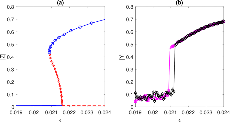
Figure 2. (a): $|Z|$ for fixed point (lines) and periodic solutions (symbols) of (16). Blue solutions are stable while red are unstable. (b): $|Y|$ for the network (1). Black corresponds to increasing $\epsilon$ and magenta to decreasing. Parameters: $m=100,M=400,N=2000,\sigma=0.01,\Delta=0.0005$.

Following the Hopf bifurcation and saddle-node bifurcation of periodic orbits shown in Fig. 2(a) as both $\sigma$ and $\epsilon$ are varied we obtain Fig. 3. Although the range of values of $\epsilon$ for which the system is bistable is small, it increases as $\sigma$ is increased. We have shown that even with very different distributions of in-degrees and intrinsic frequencies, positively correlating them can induce ES in a directed network of Winfree oscillators.

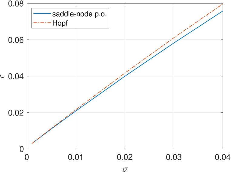
Figure 3. Curves of Hopf and saddle-node bifurcations as seen in Fig. 2(a) as both $\sigma$ and $\epsilon$ are varied. The network is bistable between the curves. Parameters: $m=100,M=400,\Delta=0.0005$.

The results of our numerical investigation into the effects of varying the correlation between the $k_{in,j}$ and $\omega_{j}$ ($\rho_{k\omega}$) are shown in Fig 4 (panels C and D). We varied $\rho_{k\omega}$ between 0.6 and 0.95 using the Monte-Carlo degree-swapping method explained above and for each network we quasistatically increased or decreased the coupling strength $\epsilon$ and measured the time-averaged value of $|Y|$. This is shown in Fig 4C where we see results similar to those in Fig. 2 — a small region of bistability. Panel D of Fig 4 shows the fraction of effective frequencies as the coupling strength is progressively increased, at $\rho_{k\omega}=0.95$.

The distribution of frequencies and their fractional evolution corresponds to the mean and standard deviation of the Gaussian distribution, and the highest concentration of frequencies around the mean emerge dominant. However, the effects of having a large value of $\rho_{k\omega}$ for Gaussian distributed intrinsic frequencies is minimal compared with that for power law distributed frequencies, considered next.

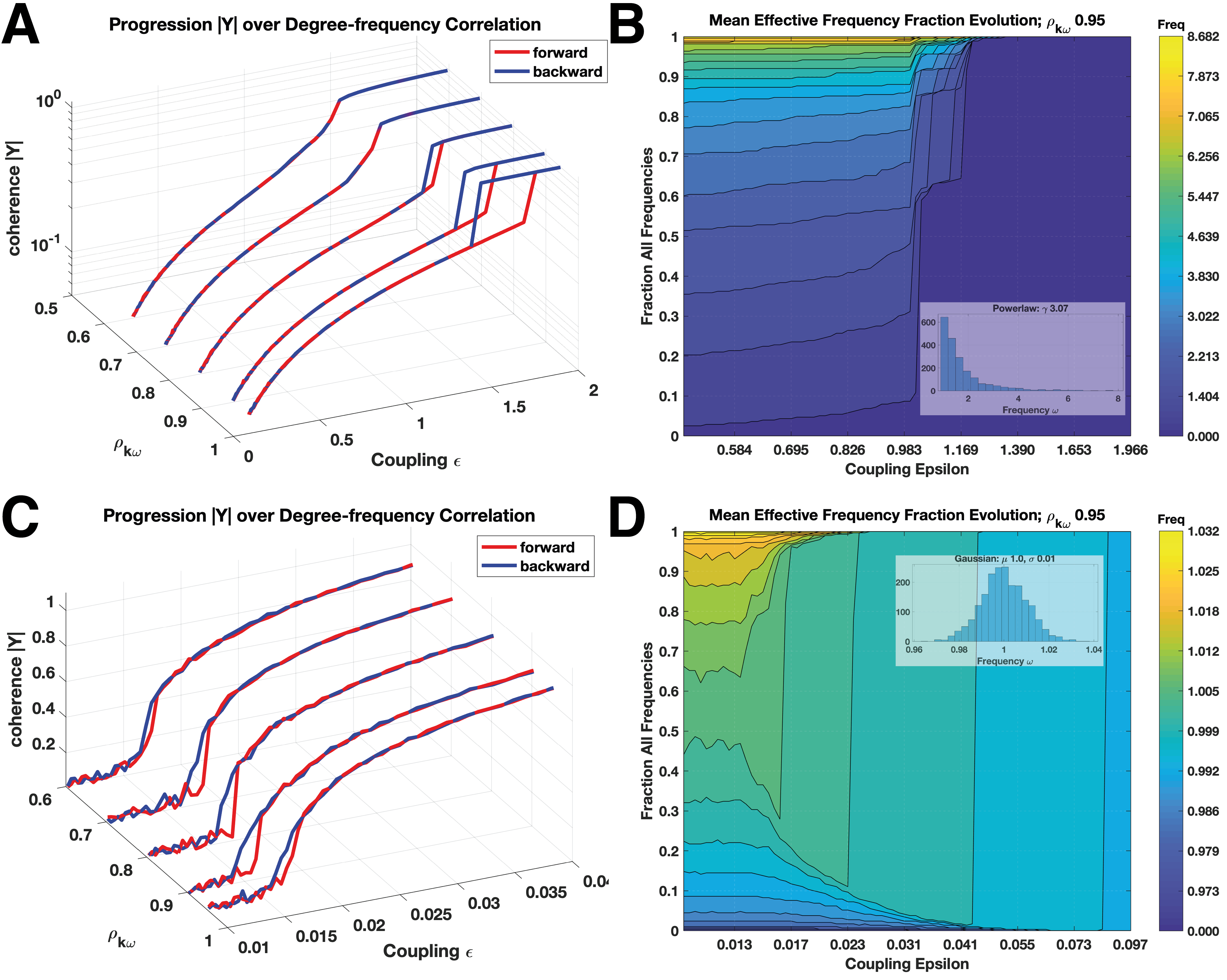
Figure 4. Panels A and C: $|Y|$ as $\epsilon$ is quasistatically varied for networks with different values of $\rho_{k\omega}$. Panels B and D: Progression of mean-effective frequency fraction distribution over increasing coupling strength $\epsilon$, for $\rho_{k\omega}$ = 0.95; note distinct colour scales for effective frequency evolution due to underlying $\omega$ distributions (histograms, insets Panels B & D), and distinct $\epsilon$ scales reflecting hysteresis over different coupling strengths. Panels A and B show results when the intrinsic frequencies are power law distributed with an exponent of $-3.07$ and in- and out-degrees drawn from power law distribution with same exponent and neutral correlation between the in- and out-degrees. Panels C and D show results for Gaussian distributed frequencies with mean $1.0$ and $\sigma=0.01$, while in- and out-degrees are power law distributed with exponent $-2.66$ and the in-degrees are highly correlated with the out-degrees ($\rho=0.89$).

4. Power law frequency distribution

We keep the power law distribution of degrees (21) and now consider the case where the target distribution frequency distribution is also power law distributed and limited between $c$ and $C$, but with the exponent as a parameter, i.e.

$$p_{\omega_{0}}(\omega_{0})=\begin{cases}a_{\omega}/\omega_{0}^{\gamma+1}&c\leq\omega_{0}\leq C\\ 0&\mbox{ otherwise}\end{cases}$$ (29)

where $a_{\omega}=\gamma c^{\gamma}C^{\gamma}/(C^{\gamma}-c^{\gamma})$. As above, having created a network we randomly choose target frequencies from the distribution (29), then assign the smallest target frequency to the oscillator with the smallest in-degree, all the way up to the largest target frequency being associated with oscillator with the largest in-degree. The actual $\omega_{j}$ are then chosen from a Lorentzian with HWHM equal to $\Delta$ centred at the target frequency, as above. The dependence of $\omega_{0}$ on $k$ is then

$$\omega_{0}(k)=\widehat{p}_{\omega_{0}}^{-1}(\widehat{p}(k))$$ (30)

where $\widehat{p}_{\omega_{0}}$ is the cumulative distribution function of $p_{\omega_{0}}$, i.e

$$\widehat{p}_{\omega_{0}}(\omega_{0})=\frac{a_{\omega}}{\gamma}\left(\frac{1}{c^{\gamma}}-\frac{1}{\omega_{0}^{\gamma}}\right)$$ (31)

4.1. Highly correlated degree and frequency

4.1.1. Independent degrees

We first consider the case of independent degrees, as in Sec. 3. Thus we numerically investigate (16) with (14), but using (30). We choose $\Delta=0.01$, set $c=1,C=6$, and initially choose $\gamma=2$. As in Sec. 3, for small $\epsilon$ the system has a stable fixed point and this becomes unstable through a subcritical Hopf bifurcation as $\epsilon$ is increased. The results are shown in Fig. 5 where we see the periodic orbit created in the Hopf bifurcation, giving the same scenario as in Fig. 2 (a). Quasistatically increasing $\epsilon$ the solution of (16) would jump from a fixed point to a periodic state with amplitude significantly larger than zero. Decreasing $\epsilon$, the solution would jump from a finite-amplitude periodic orbit to a fixed point. (As above, for periodic orbits, the quantity plotted on the vertical axis is the average over one period of $|Z(t)|$.)

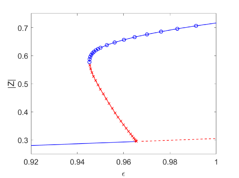
Figure 5. $|Z|$ for fixed point (lines) and periodic (symbols) solutions of (16). Blue solutions are stable while red are unstable. Parameters: $c=1,C=6,m=100,M=400,\gamma=2,\Delta=0.01$.

The behaviour of a particular realisation of the discrete network (1) is slightly different, since a fixed point of (16) corresponds to an incoherent solution of (1) for which $|Y|$ is not constant, having small fluctuations about an average value. An example of such dynamics is shown in Fig. 6(a), with $\epsilon=0.92$. (Other parameters have the same values as in Fig. 5.) We see that most oscillators are oscillating, but with independent phases. Similarly, a periodic solution of (16) corresponds to a solution of (1) for which $|Y|$ is nearly periodic, with the vast majority of the oscillators having the same average frequency, as shown in Fig. 6(b) ($\epsilon=1$). Some with high in-degree fire at multiples of this frequency and some are unlocked, giving a state referred to by [1] as “partially locked hybrid states.” See also [26] for examples of these dynamics.

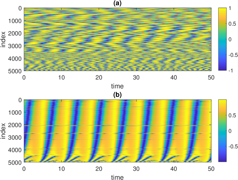
Figure 6. $\sin{\theta}$ shown in colour for a simulation of (1). The oscillators are sorted by their in-degree. (a): $\epsilon=0.92$. (b): $\epsilon=1$. Other parameters: $N=5000,c=1,C=6,m=100,M=400,\gamma=2,\Delta=0.01$.

However for $\gamma=1$ the results are very different. As seen in Fig. 7(a) the branch with the lower value of $|Z|$ still undergoes a Hopf bifurcation. Numerical integration of (16) near the bifurcation does not show a stable periodic orbit so this bifurcation seems subcritical, creating an unstable periodic orbit as $\epsilon$ is decreased. This orbit never becomes stable, and we hypothesise that it is destroyed in a homoclinic bifurcation with the “middle” unstable branch. Thus the system has no stable periodic orbits, but rather a region of bistability between two fixed points with different values of $|Z|$. Either increasing or decreasing $\epsilon$ the network jumps from one fixed point to another. Fig. 7(b) shows the mean firing rate $F$ across the network and we see that the branch with large $|Z|$ has small $F$ and vice versa. So even if $|Z|$ is large, normally indicating synchronous oscillations, here it corresponds to a state in which most of the oscillators are locked at an approximate fixed point, not firing.

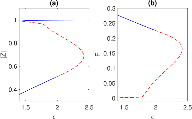
Figure 7. (a) $|Z|$ and (b) mean firing rate $F$ for fixed points of (16). Solid: stable; dashed: unstable. The bifurcation on the lower branch in (a) is a subcritical Hopf. Parameters: $c=1,C=6,m=100,M=400,\gamma=1,\Delta=0.01$.

Fig. 8 shows (on a logarithmic scale) the expected frequency for oscillators with in-degree $k_{in}$, given by (19), for three coexisting steady states in Fig. 7 at $\epsilon=1.7$. The stable solution with highest frequencies has the lowest value of $|Z|$ and vice versa. Interestingly, for the upper curve the frequency increases with in-degree $k_{in}$, but for the lower two curves the maximum frequency does not occur at either extreme of the $k_{in}$ values.

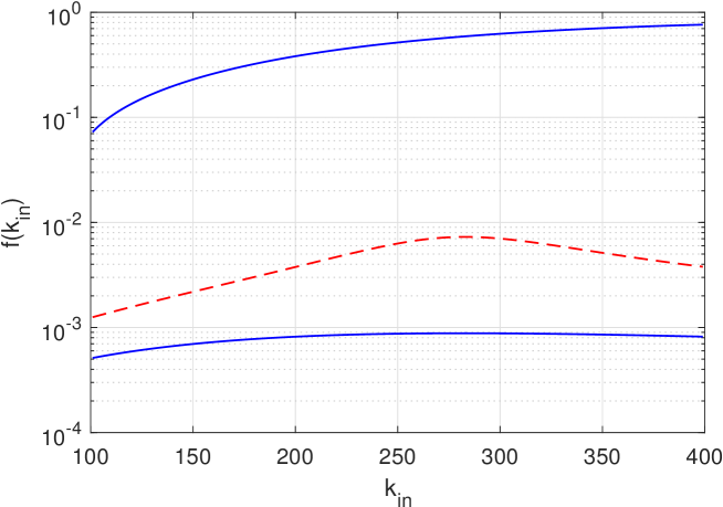
Figure 8. Expected frequency for oscillators with in-degree $k_{in}$, given by (19), for three coexisting steady states at $\epsilon=1.7$. See Fig. 7. Blue: stable solutions; red: unstable solution. Other parameters: $c=1,C=6,m=100,M=400,\gamma=1,\Delta=0.01$.

A third scenario occurs for $\gamma=1.5$, as seen in Fig. 9. The fixed point that is stable for small $\epsilon$ becomes unstable through a subcritical Hopf bifurcation as $\epsilon$ is increased as in Fig. 5, but the stable periodic orbit is destroyed in a SNIC bifurcation which occurs at a slightly lower value of $\epsilon$ than that at which the Hopf bifurcation occurs. So if $\epsilon$ is slowly increased the network will jump from one fixed point to another fixed point. But if $\epsilon$ is then decreased the network will switch from a fixed point to a stable periodic orbit. This stable orbit is then destroyed in a saddle-node bifurcation as $\epsilon$ is further decreased and the network will jump to the original fixed point.

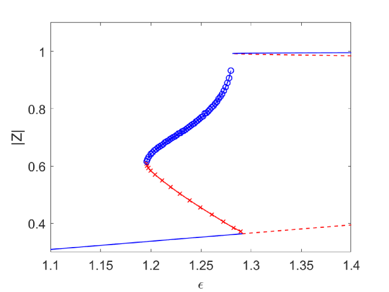
Figure 9. $|Z|$ for fixed point (lines) and periodic (symbols) solutions of (16). Blue solutions are stable while red are unstable. The stable branch of periodic orbits terminates at the SNIC bifurcation. Parameters: $c=1,C=6,m=100,M=400,\gamma=1.5,\Delta=0.01$.

4.1.2. Identical degrees

We now consider the case of identical in- and out-degrees. We numerically investigate (16) with (15), using the power law distribution of degrees (21) and the power law distribution of frequencies (29). The results for $\gamma=2$ are shown in Fig. 10. The scenario is qualitatively the same as in Fig. 9, with bistability between either two fixed points or between a fixed point and a periodic solution.

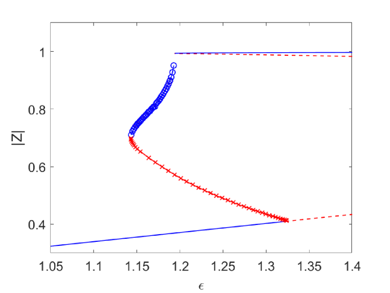
Figure 10. Identical degrees. $|Z|$ for fixed point (lines) and periodic (symbols) solutions of (16). Blue solutions are stable while red are unstable. The stable branch of periodic orbits terminates at the SNIC bifurcation. Parameters: $c=1,C=6,m=100,M=400,\gamma=2,\Delta=0.01$.

For $\gamma=1$ we obtain Fig. 11, showing yet another scenario. Here there are no Hopf bifurcations, only two saddle-node bifurcations of fixed points, with region of bistability between them.

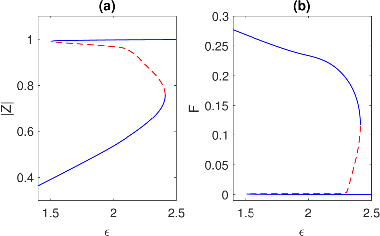
Figure 11. Identical degrees. (a) $|Z|$ and (b) mean firing rate $F$ for fixed points of (16). Solid: stable; dashed: unstable. Parameters: $c=1,C=6,m=100,M=400,\gamma=1,\Delta=0.01$.

All of the results reported in this section have been verified using simulations of the discrete network (results not shown).

4.1.3. Varying degree-frequency correlation

We repeated our numerical investigation into the effects of varying degree-frequency correlations — which we denoted $\rho_{k\omega}$ — generated via the Monte-Carlo swapping and permutation assembly method with power law distributed frequencies. The results are shown in Fig. 4 panels A and B. Increasing $\rho_{k\omega}$ corresponds with the appearance and subsequent widening of the region of hysteresis, for the power law distributed $\omega$. The Gaussian distribution (Panels C and D) alternatively demonstrates hysteresis but with narrowing at the highest level of correlation and is more sensitive to the network realisation, or final assembly of the connectivity matrix $A$ given the same degree and $\omega$ sequence. Some realisations demonstrated hysteresis but others did not with all other elements identical, and compared to the power law distributed frequencies, we observed less consistency in emergent hysteresis across the multiple network realisations. Further, the Gaussian $\omega$ results are clearly and simply noisier, partly due to the scale of plots showing hysteresis at far lower $\epsilon$ values. This is also due to the modes of synchronisation for these two $\omega$ distributions: the Gaussian with dynamic synchrony and the power law with destructive or a quiescent synchrony as observed with locking the system at fixed points of zero frequency. Note the progression of mean effective frequency distributions with increasing coupling strength (at the highest $\rho_{k\omega}=0.95$), where the power law $\omega$ system collapses into quiescence (Fig. 4 panel B) as opposed to the scenario for Gaussian distributed $\omega$ (Fig. 4 panel D). Coherence frequencies emerge at levels dictated by the concentration of $\omega$ values for each distribution: power law close to zero and Gaussian close to the mean ($\mu=1.0$).

5. Discussion

We have considered directed networks of Winfree oscillators with truncated inverse power law distributions of both in- and out-degrees. We considered the case of oscillators having independent in- and out-degrees, and also the case where they are equal. For independent degrees we examined both Gaussian and power law distributed intrinsic frequencies, having these frequencies highly correlated with oscillators’ in-degrees as a result of sorting both sets and associating quantities of equal rank. We investigated the effects of varying this degree of correlation. For identical in- and out-degrees we also considered power law distributed frequencies with a positive correlation between an oscillator’s in-degree and its intrinsic frequency. We varied both the width of the Gaussian frequency distribution (when used) and the exponent in the power law frequency distribution and examined the transitions that occurred as the strength of coupling within the network was varied.

In all cases shown there was an “explosive” transition as the coupling strength was varied from one fixed point to another, or between a fixed point and a periodic solution. An exception occurs with lower degree-frequency correlations for the power law frequency distributed case. A variety of scenarios were seen. This is in contrast to the similar and much more widely studied Kuramoto model, for which transitions are only between an incoherent fixed point and a partially synchronous periodic solution [6, 8]. The range of scenarios is a result of the form of a Winfree oscillator: for strong enough coupling an oscillator will approximately lock to a fixed point, so that even though the measure of synchrony $|Z|$ may increase as coupling strength is increased, this does not necessarily correspond to synchronous firing, as can be seen in Figs. 7 and 11.

Acknowledgements: This work was partially supported by the Marsden Fund Council from Government funding, managed by Royal Society Te Aparangi, grant number 17-MAU-054.

References

- [1] Joel T Ariaratnam and Steven H Strogatz. Phase diagram for the winfree model of coupled nonlinear oscillators. Physical Review Letters, 86(19):4278, 2001.
- [2] S Boccaletti, JA Almendral, S Guan, I Leyva, Z Liu, I Sendiña-Nadal, Z Wang, and Y Zou. Explosive transitions in complex networks’ structure and dynamics: Percolation and synchronization. Physics Reports, 660:1–94, 2016.
- [3] Christoph Börgers and Nancy Kopell. Synchronization in networks of excitatory and inhibitory neurons with sparse, random connectivity. Neural Computation, 15(3):509–538, 2003.
- [4] Aldo Casaleggio, Michael L Hines, and Michele Migliore. Computational model of erratic arrhythmias in a cardiac cell network: the role of gap junctions. PLoS One, 9(6):e100288, 2014.
- [5] Sarthak Chandra, David Hathcock, Kimberly Crain, Thomas M. Antonsen, Michelle Girvan, and Edward Ott. Modeling the network dynamics of pulse-coupled neurons. Chaos, 27(3):033102, 2017.
- [6] Raissa M. D’Souza, Jesus Gómez-Gardeñes, Jan Nagler, and Alex Arenas. Explosive phenomena in complex networks. Advances in Physics, 68(3):123–223, 2019.
- [7] Rafael Gallego, Ernest Montbrió, and Diego Pazó. Synchronization scenarios in the winfree model of coupled oscillators. Physical Review E, 96(4):042208, 2017.
- [8] Jesús Gómez-Gardeñes, Sergio Gómez, Alex Arenas, and Yamir Moreno. Explosive synchronization transitions in scale-free networks. Phys. Rev. Lett., 106:128701, Mar 2011.
- [9] Willy JF Govaerts. Numerical methods for bifurcations of dynamical equilibria, volume 66. Siam, 2000.
- [10] Seung-Yeal Ha, Jinyeong Park, and Sang Woo Ryoo. Emergence of phase-locked states for the winfree model in a large coupling regime. Discrete & Continuous Dynamical Systems, 35(8):3417, 2015.
- [11] Christian Kuehn and Christian Bick. A universal route to explosive phenomena. Science Advances, 7(16):eabe3824, 2021.
- [12] Y. Kuramoto. Chemical oscillations, waves, and turbulence. Springer-Verlag, 1984.
- [13] C. R. Laing. Numerical bifurcation theory for high-dimensional neural models. The Journal of Mathematical Neuroscience, 4(1):1, 2014.
- [14] Carlo R Laing. Effects of degree distributions in random networks of type-i neurons. Physical Review E, 103(5):052305, 2021.
- [15] Carlo R Laing and Christian Bläsche. The effects of within-neuron degree correlations in networks of spiking neurons. Biological Cybernetics, 114:337–347, 2020.
- [16] Carlo R Laing, Christian Bläsche, and Shawn Means. Dynamics of structured networks of winfree oscillators. Front Syst Neurosci, 15:631377, 2021.
- [17] I Leyva, A Navas, I Sendina-Nadal, JA Almendral, JM Buldú, M Zanin, D Papo, and S Boccaletti. Explosive transitions to synchronization in networks of phase oscillators. Scientific reports, 3(1):1–5, 2013.
- [18] Weiqing Liu, Ye Wu, Jinghua Xiao, and Meng Zhan. Effects of frequency-degree correlation on synchronization transition in scale-free networks. EPL (Europhysics Letters), 101(3):38002, 2013.
- [19] Tanushree B Luke, Ernest Barreto, and Paul So. Complete classification of the macroscopic behavior of a heterogeneous network of theta neurons. Neural Computation, 25:3207–3234, 2013.
- [20] Shawn A Means, Christian Bläsche, and Carlo R Laing. A permutation method for network assembly. PLoS One, 15(10):e0240888, 2020.
- [21] Sung Moon, Katherine Cook, Karthikeyan Rajendran, I. G. Kevrekidis, Jaime Cisternas, and C. R. Laing. Coarse-grained clustering dynamics of heterogeneously coupled neurons. Journal of Mathematical Neuroscience, 5(1):2, 2015.
- [22] Theoden I. Netoff, Matthew I. Banks, Alan D. Dorval, Corey D. Acker, Julie S. Haas, Nancy Kopell, and John A. White. Synchronization in hybrid neuronal networks of the hippocampal formation. Journal of Neurophysiology, 93(3):1197–1208, 2005. PMID: 15525802.
- [23] M.E.J. Newman. The structure and function of complex networks. SIAM Review, 45(2):167–256, 2003.
- [24] E. Ott and T.M. Antonsen. Low dimensional behavior of large systems of globally coupled oscillators. Chaos, 18:037113, 2008.
- [25] E. Ott and T.M. Antonsen. Long time evolution of phase oscillator systems. Chaos, 19:023117, 2009.
- [26] Diego Pazó and Ernest Montbrió. Low-dimensional dynamics of populations of pulse-coupled oscillators. Physical Review X, 4(1):011009, 2014.
- [27] Diego Pazó, Ernest Montbrió, and Rafael Gallego. The winfree model with heterogeneous phase-response curves: analytical results. Journal of Physics A: Mathematical and Theoretical, 52(15):154001, 2019.
- [28] V. Pernice, B. Staude, S. Cardanobile, and S. Rotter. How structure determines correlations in neuronal networks. PLoS Computational Biology, 7(5), 2011. cited By 117.
- [29] A. Pikovsky, M. Rosenblum, and J. Kurths. Synchronization. Cambridge University Press, 2001.
- [30] Dietmar Plenz and Stephen T Kitai. Up and down states in striatal medium spiny neurons simultaneously recorded with spontaneous activity in fast-spiking interneurons studied in cortex–striatum–substantia nigra organotypic cultures. Journal of Neuroscience, 18(1):266–283, 1998.
- [31] Juan G Restrepo and Edward Ott. Mean-field theory of assortative networks of phase oscillators. EPL (Europhysics Letters), 107(6):60006, 2014.
- [32] Nathan W Schultheiss, Astrid A Prinz, and Robert J Butera. Phase response curves in neuroscience: theory, experiment, and analysis. Springer, 2011.
- [33] Per Sebastian Skardal and Alex Arenas. Disorder induces explosive synchronization. Phys. Rev. E, 89:062811, Jun 2014.
- [34] Per Sebastian Skardal, Juan G Restrepo, and Edward Ott. Frequency assortativity can induce chaos in oscillator networks. Physical Review E, 91(6):060902, 2015.
- [35] Moira L Steyn-Ross, D Alistair Steyn-Ross, James W Sleigh, and DTJ Liley. Theoretical electroencephalogram stationary spectrum for a white-noise-driven cortex: evidence for a general anesthetic-induced phase transition. Physical Review E, 60(6):7299, 1999.
- [36] S.H. Strogatz. From Kuramoto to Crawford: exploring the onset of synchronization in populations of coupled oscillators. Physica D, 143:1–20, 2000.
- [37] Yasuhiro Tsubo, Jun-nosuke Teramae, and Tomoki Fukai. Synchronization of excitatory neurons with strongly heterogeneous phase responses. Physical review letters, 99(22):228101, 2007.
- [38] CJ Wilson and Y Kawaguchi. The origins of two-state spontaneous membrane potential fluctuations of neostriatal spiny neurons. Journal of Neuroscience, 16(7):2397–2410, 1996.
- [39] Arthur T Winfree. Biological rhythms and the behavior of populations of coupled oscillators. Journal of Theoretical Biology, 16(1):15–42, 1967.
- [40] Jinshan Xu, Shakti N Menon, Rajeev Singh, Nicolas B Garnier, Sitabhra Sinha, and Alain Pumir. The role of cellular coupling in the spontaneous generation of electrical activity in uterine tissue. PLoS One, 10(3):e0118443, 2015.
- [41] Xiyun Zhang, Stefano Boccaletti, Shuguang Guan, and Zonghua Liu. Explosive synchronization in adaptive and multilayer networks. Physical review letters, 114(3):038701, 2015.
- [42] Xiyun Zhang, Yong Zou, Stefano Boccaletti, and Zonghua Liu. Explosive synchronization as a process of explosive percolation in dynamical phase space. Scientific reports, 4(1):1–6, 2014.