Numerical analysis of ligament instability and breakup in shear flow

Abstract

In this study, we perform a numerical analysis of the instability of a ligament in shear flow and investigate the effects of air-liquid shear on the growth rate of the ligament interface, breakup time, and droplet diameter formed by the breakup. The ligament is stretched in the flow direction by the shearing of airflow. Furthermore, as the influence of the shear flow increases, the ligament becomes deformed into a liquid sheet, and a perforation forms at the center of the liquid sheet. The liquid sheet breaks up due to the growth of the perforation and contracts under the influence of surface tension, forming two ligaments with diameters smaller than that of the original ligament. The shearing of the airflow causes the original ligament to elongate, and the cross-section of the ligament becomes elliptical, which increases instability. As a result, the growth rate of the ligament exceeds the theoretical value, and increases with increasing wavenumber of the initial disturbance. Therefore, the diameter of the formed droplets in shear flow decreases due to the increase in the wavenumber that governs the breakup of the ligament, and because the growth rate increases, the breakup time for the ligament decreases. As the velocity difference of the shear flow increases, constrictions of the ligament form earlier and the diameter of the satellite droplet increases. As the diameter of the satellite droplet increases and that of the main droplet decreases, the dispersion of the droplet diameter decreases, making the diameter uniform.

I Introduction

Liquid atomization technology is used in various fields, including industry, agriculture, and medicine. In industry, atomization technology is applied in internal combustion engines, spray coating, spray drying, and powder production. Elucidation of atomization characteristics would thus help improve performance. The process of liquid atomization is not fully understood because it consists of very complicated and small-scale phenomena. Studies on the deformation and breakup of simple-shaped liquids such as liquid sheets, liquid columns, and droplets have been conducted to elucidate atomization.

In the general atomization process, as the ejected liquid (in the form of a liquid sheet or a liquid column) is destabilized by the shearing of gas and liquid, a fine-scale liquid column, called a ligament, is generated and the liquid eventually splits into small droplets Hashimoto (1995). Theoretical studies Senecal et al. (1999); O’Rourke and Amsden (1987), experimental studies Yoshida (2000); Negeed et al. (2011), and numerical studies Li and Tankin (1991); Lozano, Olivares, and Dopazo (1998); Li, Renardy, and Renardy (2000); Kan and Yoshinaga (2007) have been conducted on the destabilization of liquid sheets and droplets. Although many studies on the destabilization of liquid columns and cylindrical liquid jets have been reported Rayleigh (1878); Weber (1931); Donnelly, Glaberson, and Chandrasekhar (1966); Yuen (1968); Goedde and Yuen (1970); Rutland and Jameson (1971); Lafrance (1975); Sterling and Sleicher (1975); Hoyt and Taylor (1977); Tjahjadi, Stone, and Ottino (1992); Park, Yoon, and Heister (2006); Kasyap, Sivakumar, and Raghunandan (2009); Hoeve et al. (2010); Lakdawala, Thaokar, and Sharma (2015); Wang and Fang (2015), few studies have been conducted on fine-scale ligaments, and thus the destabilization of ligaments is not fully understood.

In previous studies Fraser et al. (1962); Dombrowski and Johns (1963), the instability of a ligament formed in the atomization process is often considered based on the linear theory of the instability of a stationary liquid column Rayleigh (1878). Rayleigh’s theory does not consider the effects of viscosity and surrounding fluids. The instability of a liquid column in consideration of viscosity Weber (1931); Sterling and Sleicher (1975); Lakdawala, Thaokar, and Sharma (2015) and the instability of a cylindrical liquid jet due to the shearing of gas and liquid Hoyt and Taylor (1977) have been investigated.

In a study of cylindrical liquid jets Hoyt and Taylor (1977), the formation of small-scale liquid columns was observed at the interface of the liquid column destabilized by velocity shear. The breakup of this fine-scale secondary liquid column (ligament) generates droplets. When an external force such as velocity shear acts on a liquid that is not limited to a liquid column (i.e., it is a continuum), turbulence occurs inside the liquid. The growth of this turbulence deforms the liquid interface, leading to the formation of fine ligaments Hashimoto (1995); Sallam, Dai, and Faeth (1999). Finally, fine sprays form due to the repeated breakup of ligaments and droplets. Therefore, the breakup characteristics of ligaments should be investigated to clarify spray characteristics.

In the high-speed flow field in an atomizer, because both the gas and liquid flows are turbulent, the turbulence intensity at the gas-liquid interface increases with time. In such a flow field, the airflow around a ligament is not uniform; instead, it is shear flow with a velocity gradient. In this case, because the ligament is deformed by the shear flow, the breakup time and droplet diameter will be different from those of a ligament in a stationary fluid or a uniform airflow. However, the behavior of a ligament in turbulent flow and the effect of shear flow on the instability of a ligament have not been sufficiently investigated.

To clarify the behavior of a ligament in turbulent flow, we perform a numerical analysis of a ligament in shear flow and investigate the effects of gas-liquid shear on the growth rate at the ligament interface, break time, and droplet size.

II Numerical Procedures

This study considers incompressible viscous flow. We apply the level set method to track the interface Sussman, Smereka, and Osher (1994). In addition, the continuum surface force method Brackbill, Kothe, and Zemach (1992) is used to evaluate the surface tension, which is treated as the body force. The governing equations for incompressible two-phase flow are the continuity equation, the Navier-Stokes equation, the advection equation for the level set function, and the reinitialization equation, which are given as follows:

$$\nabla\cdot{\bf u}=0,$$ (1)

$$\frac{\partial{\bf u}}{\partial t}+\nabla\cdot({\bf u}{\bf u})=\frac{1}{\rho}\left[-\nabla p+\frac{1}{Re}\nabla\cdot(2\mu{\bf D})+\frac{1}{We}\kappa\hat{\bf n}\delta_{s}\right],$$ (2)

$$\frac{\partial\phi}{\partial t}+{\bf u}\cdot\nabla\phi=0,$$ (3)

$$\frac{\partial\phi}{\partial\tau}+{\bf V}\cdot\nabla\phi=S(\phi_{0}),$$ (4)

$${\bf V}=S(\phi_{0})\frac{\nabla\phi}{|\nabla\phi|},$$ (5)

where $t$ is time, ${\bf u}=(u,v,w)$ is the velocity vector at the coordinates ${\bf x}=(x,y,z)$, $\rho$ is the density, $p$ is the pressure, $\mu$ is the viscosity coefficient, and ${\bf D}$ is the strain rate tensor. $\kappa$ is the interface curvature, $\hat{\bf n}$ is the unit normal vector at the interface, $\delta_{s}$ is the delta function, and $\phi$ is the level set function. $\phi_{0}$ is the level set function before reinitialization. The variables in the fundamental equations are non-dimensionalized as follows using the reference values of length $L_{\mathrm{ref}}$, velocity $U_{\mathrm{ref}}$, density $\rho_{\mathrm{ref}}$, and viscosity coefficient $\mu_{\mathrm{ref}}$:

$$t^{*}=\frac{U_{\mathrm{ref}}t}{L_{\mathrm{ref}}}\ ,\quad{\bf x}^{*}=\frac{\bf x}{L_{\mathrm{ref}}}\ ,\quad{\bf u}^{*}=\frac{\bf u}{U_{\mathrm{ref}}}\ ,\quad p^{*}=\frac{p}{\rho U_{\mathrm{ref}}^{2}}\ ,\quad\phi^{*}=\frac{\phi}{L_{\mathrm{ref}}},\quad$$

$$\rho^{*}=\frac{\rho}{\rho_{\mathrm{ref}}}\ ,\quad\mu^{*}=\frac{\mu}{\mu_{\mathrm{ref}}}\ ,$$ (6)

where the superscript $*$ represents a dimensionless variable and is omitted in the above governing equations. As dimensionless parameters in these equations, $Re=U_{\mathrm{ref}}L_{\mathrm{ref}}/\nu$ is the Reynolds number, $We=\rho_{\mathrm{ref}}L_{\mathrm{ref}}U_{\mathrm{ref}}^{2}/\sigma$ is the Weber number, and $\sigma$ is the surface tension coefficient. The strain rate tensor is defined as

$${\bf D}=\frac{1}{2}\left[\nabla{\bf u}+(\nabla{\bf u})^{T}\right].$$ (7)

The density and viscosity coefficients for the gas-liquid two-phase flow are expressed as

$$\rho=\rho_{g}+(\rho_{l}-\rho_{g})H(\phi),\quad\mu=\mu_{g}+(\mu_{l}-\mu_{g})H(\phi),$$ (8)

where the subscripts $l$ and $g$ represent liquid and gas, respectively. $H(\phi)$ is the Heaviside function and is given as

$$H(\phi)=\left\{\begin{array}[]{ll}1&\quad\mbox{if}\quad\phi>\epsilon,\\ 0&\quad\mbox{if}\quad\phi<-\epsilon,\\ \displaystyle\frac{\phi+\epsilon}{2\epsilon}+\frac{1}{2\pi}\sin\left(\frac{\pi\phi}{\epsilon}\right)&\quad\mbox{if}\quad|\phi|\leq\epsilon.\end{array}\right.$$ (9)

The gas-liquid interface is represented as a transition region with a thickness of $2\varepsilon$, where $\varepsilon$ is set to $1.0-2.0$ times the grid width. The interface curvature and the unit normal vector are expressed as

$$\kappa=-\nabla\cdot\hat{\bf n},$$ (10)

$$\hat{\bf n}=\frac{\nabla\phi}{|\nabla\phi|}.$$ (11)

The delta function at the interface is obtained as the gradient of the Heaviside function as follows:

$$\delta_{\mathrm{s}}=\nabla_{\phi}H(\phi)=\left\{\begin{array}[]{ll}0&\quad\mbox{if}\quad|\phi|>\epsilon,\\ \displaystyle\frac{1}{2\epsilon}\left[1+\cos\left(\frac{\pi\phi}{\epsilon}\right)\right]&\quad\mbox{if}\quad|\phi|\leq\epsilon.\end{array}\right.$$ (12)

The simplified marker and cell method Amsden and Harlow (1970) is used to solve Eqs. (1) and (2). The Crank-Nicholson method is used to discretize the time derivatives, and time marching is performed. The second-order central difference scheme is used for the discretization of the space derivatives. For the discretization of Eq. (3), the Crank-Nicholson method is applied for the time derivative and the fifth-order weighted essentially non-oscillatory (WENO) scheme Jiang and Peng (2000) is applied for the space derivatives. For Eq. (4), the total variation diminishing Runge-Kutta method with third-order accuracy Shu and Osher (1988, 1989) is applied for the time derivative and the fifth-order WENO scheme Jiang and Peng (2000) is applied for the space derivatives.

III Calculation Conditions

III.1 Comparison with theoretical solution

In this study, we first analyze the instability of the interface of a stationary ligament to verify the validity of the above calculation method for phenomena in which surface tension has a great effect. A cylindrical coordinate system is used for the analysis, and an axisymmetric ligament is considered. The origin is placed on the central axis of a ligament with diameter $d$. The direction of the central axis is the $x$-axis and the radial direction is the $r$-axis. A disturbance $\eta$, which is a cosine function with a small initial amplitude $\eta_{0}$, is applied to the surface of the ligament with radius $a$.

$$\eta=\eta_{0}\cos(2\pi x/\lambda),$$ (13)

where $k=2\pi/\lambda$ is the wavenumber and $\lambda$ is the wavelength. The interface of the stationary ligament fluctuates due to the influence of this disturbance. This study varies the wavenumber $k$ of the initial disturbance and compares the growth rate of the interface for each wavenumber with the theoretical value for the liquid column Rayleigh (1878); Weber (1931). We perform axisymmetric two-dimensional analyses for inviscid and viscous fluids.

The calculation region is $\lambda$ in the axial direction and $2a$ in the radial direction. Three uniform grids, with dimensions of $81\times 26$ (grid1), $101\times 51$ (grid2), and $121\times 101$ (grid3) are used for the calculations. The minimum grid widths are $0.04d$, $0.02d$, and $0.01d$, respectively. As described later, in the analyses for inviscid and viscous fluids, we confirmed that appropriate results are obtained even with the dimensions of grid2 and grid1.

Regarding the initial conditions in this calculation, the fluid is stationary, and a small disturbance with an initial amplitude of $\eta_{0}$ is applied to the interface. Periodic boundary conditions for velocity are applied at $x=0$ and $\lambda$, symmetry conditions are assumed at $r=0$, and slip boundary conditions are applied at $r=2a$. For the level set function, periodic boundary conditions are applied at $x=0$ and $\lambda$, symmetry conditions are assumed at $r=0$, and the boundary value at $r=2a$ is obtained by extrapolation.

In our calculation, the diameter of the ligament is $d=1.0\times 10^{-5}$ m. The liquid is a light oil and the surrounding gas is air. The densities of the liquid and gas are $\rho_{l}=851$ kg/m³ and $\rho_{g}=1.20$ kg/m³ and the viscosity coefficients are $\mu_{l}=2.225\times 10^{-3}$ Pa s and $\mu_{g}=1.827\times 10^{-5}$ Pa s, respectively. The surface tension coefficient is $\sigma=2.44\times 10^{-2}$ N/m. The reference values used in the calculation are $L_{\mathrm{ref}}=d$ and $U_{\mathrm{ref}}=d[\sigma/(\rho_{l}d^{3})]^{1/2}$. The dimensionless time $T$ is $T=t/(\rho_{l}d^{3}/\sigma)^{1/2}$ and the Weber number $We$ is $We=1.0$. In the calculation considering viscosity, the Ohnesorge number, which is defined as $Oh=\mu_{l}/(\rho_{l}\sigma L_{\mathrm{ref}})^{1/2}$, is set to $Oh=0.15$. Under these conditions, the Reynolds number is $Re=6.67$. The time intervals used in the calculation are $\Delta t/(d/U_{\mathrm{ref}})=8.0\times 10^{-4}$, $4.0\times 10^{-4}$, and $2.0\times 10^{-4}$ for grid1, grid2, and grid3, respectively. Calculations are performed for dimensionless wavenumbers $ka=0.3$, 0.5, 0.7, and 0.9, and the growth rate of the ligament interface at each wavenumber is compared with the theoretical results for a liquid column Rayleigh (1878); Weber (1931). The growth rate $\omega_{0}$ of the interface for the inviscid liquid column is defined by linear theory as

$$\omega_{0}^{2}=\frac{\sigma}{\rho_{l}a^{3}}\frac{\alpha I_{1}(\alpha)}{I_{0}(\alpha)}(1-\alpha^{2}),$$ (14)

where $\alpha=ka$ and $In(\alpha)$ is a modified Bessel function of the first kind. The dimensionless growth rate $\Omega_{0}$ is defined as $\Omega_{0}=\omega_{0}/[\sigma/(\rho_{l}a^{3})]^{1/2}$. From linear theory, the growth rate $\omega$ of the interface for the viscous liquid column is defined as

$$\omega^{2}+\frac{3\mu_{l}\alpha^{2}}{\rho_{l}a^{2}}\omega=\frac{\sigma}{2\rho_{l}a^{3}}(1-\alpha^{2})\alpha^{2}.$$ (15)

The dimensionless growth rate $\Omega$ is defined as $\Omega=\omega/[\sigma/(\rho_{l}a^{3})]^{1/2}$.

To examine the effect of the initial amplitude on the growth of the interface, the results obtained using three amplitudes ($\eta_{0}/d=0.01$, 0.001, and 0.0001) were compared. There was no difference in the results for $\eta_{0}/d\leq 0.01$. It was found that $\eta_{0}/d=0.01$ was sufficiently small. Therefore, the results obtained using $\eta_{0}/d=0.01$ are shown below.

III.2 Instability analysis of ligament in shear flow

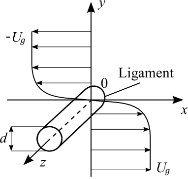
Figure 1: Flow configuration and coordinate system for ligament in shear flow

Next, we investigate the instability of a ligament in a shear flow. Figure 1 shows the flow configuration and coordinate system for this ligament. The origin is placed on the central axis of a ligament with diameter $d$. The horizontal direction is the $x$-axis, the vertical direction is the $y$-axis, and the central axis of the ligament is the $z$-axis. The gas moves in the positive and negative directions of the $x$-axis at a velocity $U_{g}$ on the lower and upper sides of the ligament, respectively. The velocity difference of the shear flow is $\Delta U=2U_{g}$. An initial disturbance with wavelength $\lambda$ is applied to the surface of the ligament.

The calculation region is $10d$ in the $x$-axis direction, $8d$ in the $y$-axis direction, and $\lambda$ in the $z$-axis direction. In the analysis described in subsection III.1, appropriate results were obtained even with the minimum grid width of grid1 in the two-dimensional viscous analysis. Thus, in this three-dimensional viscous analysis, we use a non-uniform grid with dimensions of $159\times 141\times 81$ (grid2) and a minimum grid width of $0.04d$. Using grids with dimensions of $103\times 87\times 41$ (grid1) and $209\times 197\times 101$ (grid3) and minimum grid widths of $0.08d$ and $0.02d$, respectively, we analyzed the behavior of the interface in the shear flow and confirmed that there is no grid dependence on the interface and velocity distributions. The droplet diameter after ligament breakup is compared with the results of previously reported experiments and calculations to show the validity of our calculation results.

As the initial condition in this calculation, the following velocity is applied to the gas:

$$u=-U_{g}\tanh(y/\delta),$$ (16)

where $\delta$ is a parameter related to the velocity boundary layer thickness. In this study, we set $\delta/d=0.5$ and set the velocity boundary layer thickness to about the radius of the ligament so that the entire ligament is in an airflow with a velocity gradient.

This study defines the dimensionless velocity difference as $\Delta U^{*}=\Delta U/U_{\mathrm{ref}}$ by non-dimensionalizing the velocity difference $\Delta U$ using the reference velocity $U_{\mathrm{ref}}$, as described later. The gas velocity difference $\Delta U$ in this study is determined by referring to previous diesel spray experiments Arai and Hiroyasu (1993); Suh, Park, and Lee (2007); Suh and Lee (2008); Kim and Lee (2008); Zama, Ochiai, and Arai (2012). The velocity of droplets in diesel spray depends on the injection pressure and atmospheric density. It is approximately 0-100 m/s for a low-speed spray and 0-200 m/s for a high-speed spray. In this study, we set $\Delta U=0$, 10, 20, 40, 60, 80, and 100 m/s for incompressible flow. The dimensionless velocity difference is $\Delta U^{*}=0$, 5.9, 11.9, 23.7, 35.6, 47.4, and 59.2, respectively.

As in the previous subsection, an initial disturbance with a small amplitude $\eta_{0}$ is applied to the surface of the ligament. Regarding the boundary conditions for the velocity and level set function, periodic boundary conditions are given for the $x$- and $z$-axes. At the upper and lower boundaries in the $y$-axis direction, uniform flow velocities $-U_{g}$ and $U_{g}$ are given, respectively, and the level set function is extrapolated.

In this calculation, the liquid is a light oil and the gas is air. The physical properties are the same as those described in subsection III.1. The reference values of length and velocity are defined as $L_{\mathrm{ref}}=d$ and $U_{\mathrm{ref}}=[\sigma/(\rho_{l}d^{3})]^{1/2}$, respectively, and the Ohnesorge number is defined as $Oh=\mu_{l}/(\rho_{l}\sigma L_{\mathrm{ref}})^{1/2}$.

In our calculation, the ligament diameter is determined by back calculation from the droplet diameter using linear theory Rayleigh (1878). The diameter of a droplet formed by the atomizer depends on several factors, such as the nozzle diameter, injection pressure, and nozzle shape, but is generally about $1.0\times 10^{-5}$ $-2.0\times 10^{-4}$ m Tamaki, Shimizu, and Hiroyasu (2001); Lee and Park (2002); Liu et al. (2006); Suh, Park, and Lee (2007); Suh and Lee (2008); Kim and Lee (2008). In linear theory Rayleigh (1878), the relationship between the diameter $d$ of the liquid column and the diameter $d_{\mathrm{drop}}$ of the droplet is expressed as $d_{\mathrm{drop}}=1.89d$. From this, the ligament diameter is $d=5.3\times 10^{-6}$-$1.0\times 10^{-4}$ m. In this calculation, the ligament diameter is set to $d=1.0\times 10^{-5}$ m. Then, the Reynolds number, Weber number, and Ohnesorge number are $Re=6.67$, $We=1.0$, and $Oh=0.15$, respectively. The time interval used in the calculation is $\Delta t/(d/\Delta U)=0.0005$.

IV Results and Discussion

IV.1 Comparison with theoretical solution

To investigate the growth rate of the ligament interface, Fig. 2 shows the time variation of the amplitude of the interface. The results for inviscid and viscous ligaments are shown on the left and right sides, respectively. The amplitude is the average value of the amplitudes at the center and end of the ligament. At all wavenumbers, the amplitude of the interface increases exponentially with time. The growth of the interface amplitude is the fastest at $ka=0.7$ and the slowest at $ka=0.3$. The growth of the interface of the viscous ligament is slower overall than that of the inviscid ligament.

(a) inviscid ligament

(b) viscous ligament

Figure 2: Time variations of amplitude for stationary ligament

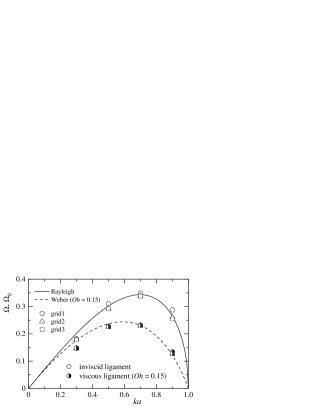
Figure 3: Growth rate of interface for stationary ligament

The validity of our calculation method is verified by comparing the growth rate of the ligament interface with the theoretical values Rayleigh (1878); Weber (1931). Figure 3 compares the dimensionless growth rates $\Omega_{0}$ and $\Omega$ obtained using each grid with the theoretical values Rayleigh (1878); Weber (1931). In the analysis for the inviscid ligament, the calculation results using the three grids agree well with the theoretical values at all wavenumbers. In the analysis for the viscous ligament, the calculation results at all wavenumbers agree well with the theoretical values, and there is no difference in the results using the three grids. Our calculation method captures the behavior of the ligament under consideration of viscosity even with the dimensions of grid1. These results indicate that the behavior of the ligament interface deformed by surface tension was captured in this analysis and that grid2 had sufficient resolution.

IV.2 Deformation of ligament due to shear flow

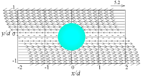
(a) $T=0$

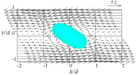
(b) $T=0.1$

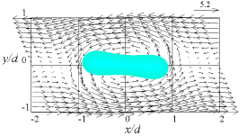
(c) $T=0.3$

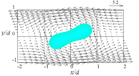
(d) $T=0.5$

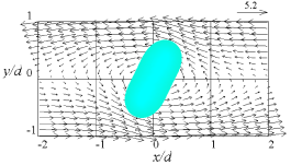
(e) $T=0.7$

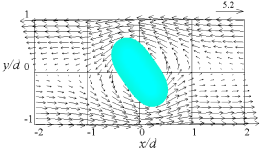
(f) $T=0.9$

Figure 4: Time variations of ligament interface and velocity vectors for $\Delta U^{*}=11.9$

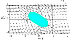
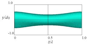
(a) $T=1.0$

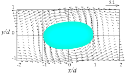
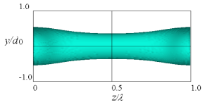
(b) $T=2.0$

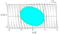
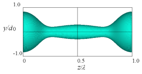
(c) $T=3.0$

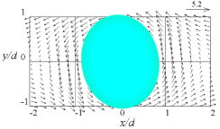
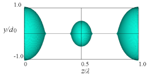
(d) $T=4.0$

Figure 5: Time variations of ligament interface and velocity vectors for $\Delta U^{*}=11.9$

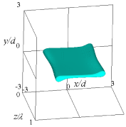
(a) $T=0.3$

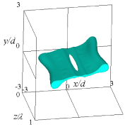
(b) $T=0.6$

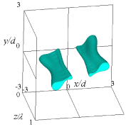
(c) $T=0.7$

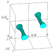
(d) $T=1.2$

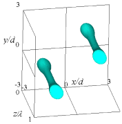
(e) $T=1.5$

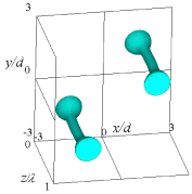
(f) $T=1.8$

Figure 6: Time variations of interface for $\Delta U^{*}=23.7$

First, we investigate the deformation of a ligament due to shear flow. Figure 4 shows the time variation of the flow field and ligament at $ka=0.7$ and $\Delta U^{*}=11.9$. Here, the interface distribution and velocity field near $z/\lambda=1.0$ are shown. At $T=0-0.3$, the ligament is stretched in the $x$-direction by the shear of the airflow. At that time, the airflow is along the interface of the ligament. As a result, after $T=0.5$, the ligament rotates counterclockwise. At $T=0.9$, the cross-section of the ligament is elliptical.

The time variation of the flow field and ligament after $T=1.0$ for $ka=0.7$ and $\Delta U^{*}=11.9$ is shown in Fig. 5. The figure on the left shows the interface distribution and velocity field near $z/\lambda=1.0$, and the figure on the right shows a side view of the ligament. The ligament interface grows with time and the ligament eventually breaks up. The position of the ligament interface at $x/d=0$ oscillates up and down. The radius at the center of the ligament decreases with time. In each side view at $T=1.0$ and 2.0, the interface distribution has a cosine-like form and a constriction is generated at the center of the ligament. At $T=3.0$, the interface disturbance grows in a non-cosine manner, and the interface near $z/\lambda=0.25$ and 0.75 is constricted. As a result, the ligament does not break up in the center; instead, it breaks up around $z/\lambda=0.25$ and 0.75. At $T=4.0$, a small-scale droplet forms between the droplets at both ends. The small droplet in the center is called a satellite droplet. The formation of satellite droplets has been confirmed in previous experiments and numerical analyses for slow jets Goedde and Yuen (1970); Rutland and Jameson (1971); Lakdawala, Thaokar, and Sharma (2015). In this study, the droplets at the two ends are referred to as the main droplets.

Figure 6 shows the time variation of the ligament interface at $\Delta U^{*}=23.7$. At $T=0.3$, the ligament is stretched in the $x$-direction by the shear of the airflow and is deformed into a liquid sheet. At $T=0.6$, a perforation forms at the center of the liquid sheet due to the initial disturbance at the interface. The growth of this perforation causes a breakup at $x/d=0$. Because the split liquid sheet contracts due to surface tension, two ligaments with diameters smaller than that of the original ligament are generated at $T=1.2$. After $T=1.2$, the interfaces of these ligaments also grow with time. It is considered that these ligaments break up again, resulting in the formation of smaller droplets and an increase in the number of droplets. For $\Delta U^{*}>23.7$, the transformation to a liquid sheet, the breakup of the liquid sheet, and the subsequent formation of ligaments are similar to those shown in Fig. 6.

The time variation of the height of the ligament interface at $x/d=0$ near $z/\lambda=1.0$ for $\Delta U^{*}=23.7$, 35.6, 47.4, and 59.2 is shown in Fig. 7. Here, the results up to the time when the ligament breakup occurs at $x/d=0$ are shown. The thickness of the liquid sheet is asymptotic to a constant value for all $\Delta U^{*}$. It can be seen that the breakup time for the liquid sheet becomes shorter as $\Delta U^{*}$ increases.

Figure 7: Time variations of interface position at $ka=0.7$ for $\Delta U^{*}=23.7$, 35.6, 47.4, and 59.2

The ligament formed after the liquid sheet splits becomes unstable again under the influence of the shear of the airflow. Therefore, in the following, we consider the conditions under which the ligament does not split again into liquid sheets and investigate the effect of shear flow on the growth rate of the ligament and the breakup for $\Delta U^{*}=0$, 5.9, and 11.9.

IV.3 Variation in growth rate of ligament due to shear flow

(a) denormalized distributions

(b) normalized distributions

Figure 8: Time variations of cross–sectional averaged axial velocity for $\Delta U^{*}=0$, 5.9, and 11.9

To investigate the flow in the ligament, the time variation of the axial velocity averaged in the cross-section in the ligament at $z/\lambda=0.75$ for $ka=0.7$ and $\Delta U^{*}=0$, 5.9, and 11.9 is shown in Fig. 8(a). Figure 8(b) shows the values of the axial velocity $w$ in Fig. 8(a) non-dimensionalized by the axial velocity $w_{0}$ at $\Delta U^{*}=0$. As the interface grows, the liquid near the center of the ligament moves to the end of the ligament. As a result, in Fig. 8(a), $w$ increases with time. In addition, $w$ at each time increases as $\Delta U^{*}$ increases. It can be seen from this result that the velocity of the liquid moving from the central part of the ligament to the end part increases, and the growth of the interface becomes faster. In Fig. 8(b), $w$ at $\Delta U^{*}=5.9$ and 11.9 is significantly higher than that at $\Delta U^{*}=0$. The distributions at $\Delta U^{*}=5.9$ and 11.9 have maximum values around $T=0.4$ and 0.6, respectively. This is because cross-sections of the ligament at $\Delta U^{*}=5.9$ and 11.9 become elliptical between $T=0-0.4$ and $T=0-0.6$, respectively, and the destabilization increased. At $\Delta U^{*}=5.9$, the cross-section gradually becomes circular again, so the increase in $w$ subsides. However, at $\Delta U^{*}=11.9$, the cross-section of the ligament is elliptical even after $T=0.6$, so $w$ increases significantly.

Figure 9: Time variations of amplitude at $\Delta U^{*}=0$, 5.9, and 11.9 for $ka=0.7$

Figure 9 shows the time variation of the amplitude of the disturbance at the interface for $ka=0.7$ and $\Delta U^{*}=0$, 5.9, and 11.9 to investigate the growth rate of the ligament interface. Because the cross-section of the ligament affected by the shear flow is non-circular, the amplitude $\eta/d$ of the ligament interface is calculated using the following equation:

$$\eta/d=r_{\mathrm{eq}}/d-r_{0}/d,$$ (17)

where $r_{\mathrm{eq}}$ is the equivalent radius of the circle obtained from the cross-sectional area of the ligament, $r_{0}$ is the radius of the ligament when no initial disturbance is applied, and $r_{0}/d=0.5$. The dimensionless growth rates at $\Delta U^{*}=0$, 5.9, and 11.9 are 0.22, 0.30, and 0.61, respectively, and the growth of the disturbance amplitude becomes faster as $\Delta U^{*}$ increases.

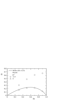
Figure 10: Growth rate of interface for $\Delta U^{*}=0$ and 11.9

In Fig. 10, the variation of the dimensionless growth rate $\Omega$ with the wavenumber $ka$ at $\Delta U^{*}=0$ and 11.9 is compared with the theoretical value Weber (1931). The growth rate of the ligament interface at $\Delta U^{*}=0$ agrees well with the theoretical value and it is the highest at $ka=0.7$. In contrast, at $\Delta U^{*}=11.9$, the growth rate is higher than the theoretical value, and that at $ka=0.9$ is higher than that at $ka=0.7$. In a previous study Rayleigh (1878), the growth rate of a liquid column in a stationary fluid was the highest at $ka=0.7$. Thus, the wavenumber that governs the breakup of a liquid column was $ka=0.7$. However, in a shear flow, the growth rate of the ligament is higher than the theoretical value, and increases with increasing wavenumber. Therefore, the formed droplet diameter in the shear flow decreases due to the increase in the wavenumber that governs the breakup of the ligament, and because the growth rate increases, the breakup time for the ligament becomes shorter.

IV.4 Effect of shear flow on ligament breakup

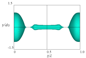
(a) $ka=0.3$ ($T=7.2$)

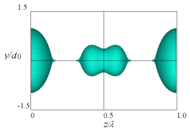
(b) $ka=0.5$ ($T=4.8$)

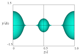
(c) $ka=0.7$ ($T=3.9$)

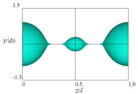
(d) $ka=0.9$ ($T=3.7$)

Figure 11: Side view of ligament interface for $\Delta U^{*}=11.9$

Next, we investigate the effect of shear flow on ligament breakup. Figure 11 shows the interface distribution immediately after breakup at wavenumbers $ka=0.3$, 0.5, 0.7, and 0.9 for $\Delta U^{*}=11.9$. The dimensionless time at each wavenumber is $T=7.2$, 4.8, 3.9, and 3.7, respectively. Satellite droplets are generated at all wavenumbers. At $ka=0.3$, a ligament forms between the main droplets. This ligament contracts with time and eventually becomes a droplet.

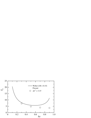
Figure 12: Breakup time variations at various wavenumbers for $\Delta U^{*}=11.9$

For $\Delta U^{*}=11.9$, the time at which breakup was confirmed at each wavenumber was taken as the breakup time $T_{b}$ in this calculation. A comparison with the breakup time for the ligament predicted using linear theory Weber (1931) is shown in Fig. 12. The predicted value was obtained by assuming that the ligament breaks up when the interface amplitude at each wavenumber grows and becomes equal to the radius of the ligament. In this analysis, the growth rate of the ligament at $\Delta U^{*}=11.9$ is higher than the theoretical value Weber (1931). Therefore, the breakup time for the ligament in this analysis is shorter than that predicted by theory.

Table 1 shows the diameter $d_{m}$ of the main droplet and the diameter $d_{s}$ of the satellite droplet at $\Delta U^{*}=0$, 5.9, and 11.9 for $ka=0.7$. In this analysis, the equivalent diameter of the droplet was calculated from the volume of the liquid in the main droplet and the satellite droplet. As $\Delta U^{*}$ increases, the diameter of the satellite droplet increases and that of the main droplet decreases.

Table 1: Droplet size at $ka=0.7$ for $\Delta U^{*}=0$, 5.9, and 11.9

velocity difference $\Delta U^{*}$	main droplet $d_{m}/d$	satellite droplet $d_{s}/d$
0	1.87	0.318
5.9	1.858	0.4922
11.9	1.761	0.8662

Figure 13 shows the distributions of the interface, pressure, and axial velocity of the ligament at $\Delta U^{*}=0$, 5.9, and 11.9 for $ka=0.7$. Because the cross-section of the ligament affected by the shear of the airflow is non-circular, the interface distribution for the ligament at $\Delta U^{*}=5.9$ and 11.9 shows the equivalent radius of the circle obtained from the cross-sectional area of the ligament. The pressure is the distribution at $x/d=0$ and $y/d=0$ and the axial velocity is the average cross-sectional value in the ligament. The dimensionless time is $T=6.5$, 5.0, and 3.6 for $\Delta U^{*}=0$, 5.9, and 11.9, respectively, and this figure shows the result immediately before the ligament breaks up. Regarding the interface distribution of the ligament, as $\Delta U^{*}$ increases, the radius near the center of the ligament increases, and the constriction forms at an earlier time. Regarding the pressure distribution, the pressure near the constriction is the highest at $\Delta U^{*}=5.9$ and 11.9. As a result, because the liquid in the center of the ligament does not move to the end, the flow velocity in the center of the ligament is almost zero at $\Delta U^{*}=5.9$. At $\Delta U^{*}=11.9$, the pressure difference between the constricted part and the central part increases, causing flow from the vicinity of the constricted part to the central part, as shown in the velocity distribution. Based on the existence of this liquid flow, it is considered that the diameter of the satellite droplet increases at $\Delta U^{*}=11.9$. Therefore, the diameter of the satellite droplet increases because the constrictions form early at both ends of the ligament interface.

(a) interface distributions

(b) pressure distributions

(c) axial velocities

Figure 13: Time variations of ligament interface, pressure, and axial velocity distributions

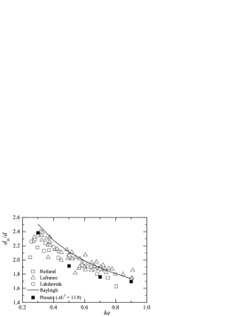
(a) main drop

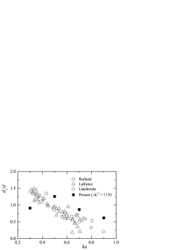
(b) satellite drop

Figure 14: Comparison of droplet diameter with previous studies for various wavenumbers

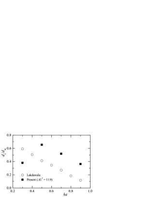
Figure 15: Comparison of drop diameter ratio with previous study for various wavenumbers

Figure 14 compares the droplet diameters obtained in this analysis with the results obtained from previous experiments on slow jets Rutland and Jameson (1971); Lafrance (1975) and a numerical analysis Lakdawala, Thaokar, and Sharma (2015). Figure 14(a) shows the diameter of the main droplet and Fig. 14(b) shows the diameter of the satellite droplet. In Fig. 14(a), the solid line shows the diameter of the droplet calculated using linear theory Rayleigh (1878). In this analysis, the diameter of the main droplet formed at $\Delta U^{*}=11.9$ is smaller than that observed in previous research. The relationship between the droplet diameter and the wavenumber is consistent with previous results. In Fig. 14(b), the diameter of the satellite droplet formed at $\Delta U^{*}=11.9$ is larger than that observed in previous studies, except at $ka=0.3$. At $ka=0.3$, the diameter of the satellite droplet is smaller than that at $ka=0.5$ because the diameter of the main droplet is larger than that for other wavenumbers.

Finally, Fig. 15 compares the ratio $d_{s}/d_{m}$ (i.e., the ratio of the diameter of the satellite droplet to that of the main droplet) with results obtained in a numerical analysis for slow jets Lakdawala, Thaokar, and Sharma (2015). In this analysis, $d_{s}/d_{m}$ at $\Delta U^{*}=11.9$ is larger than that reported in a previous study except at $ka=0.3$. The diameters of the main droplet and satellite droplet are close to each other. This indicates that the ligament breaks up under the influence of the shear of the airflow, resulting in a decrease in the dispersion of the droplet diameter and homogenization of the diameter.

V Conclusion

In this study, we performed a numerical analysis of the instability of a ligament in shear flow and investigated the effects of gas-liquid shear on the growth rate of the ligament interface, breakup time, and droplet diameter formed by the breakup. The following findings were obtained.

The ligament is stretched in the flow direction by the shear of the airflow. As the influence of the shear flow increases, the ligament deforms into a liquid sheet and a perforation forms at the center of the liquid sheet. The liquid sheet breaks up due to the growth of the perforation and contracts under the influence of surface tension, forming two ligaments with diameters smaller than that of the original ligament.

The shear of the airflow causes the original ligament to elongate, and the cross-section of the ligament becomes elliptical, which increases the instability. As a result, the growth rate of the ligament exceeds the theoretical value, and increases as the wavenumber of the initial disturbance increases. Therefore, the diameter of the formed droplet in shear flow decreases due to the increase in the wavenumber that governs the breakup of the ligament, and because the growth rate increases, the breakup time for the ligament becomes shorter.

As the velocity difference in the shear flow increases, constrictions of the ligament form earlier, and the diameter of the satellite droplet increases. As the diameter of the satellite droplet increases and the diameter of the main droplet decreases, the variation in the droplet diameter decreases, and the diameter becomes uniform.

Author Declarations

Conflicts of Interest: The authors have no conflicts to disclose.

Author Contributions: H. Y. conceived and planned the research, and developed the calculation method and numerical codes. K. N. performed the simulations. H. Y. and K. N. contributed equally to analyzing data, reaching conclusions, and writing the paper.

References

- Hashimoto (1995) H. Hashimoto, “Hydrodynamic discussion for liquid breakup mechanism,” Atomization: J. ILASS-Japan 4-2, 2–13 (1995), (in Japanese).
- Senecal et al. (1999) P. K. Senecal, D. P. Schmidt, I. Nouar, C. J. Rutland, R. D. Reitz, and M. L. Corradini, “Modeling high-speed viscous liquid sheet atomization,” Int. J. Multiph. Flow 25, 1073–1097 (1999).
- O’Rourke and Amsden (1987) P. J. O’Rourke and A. A. Amsden, “The TAB method for numerical calculation of spray droplet breakup,” in 1987 SAE International Fall Fuels and Lubricants Meeting and Exhibition, Technical Paper 872089 (SAE International in United States, 1987).
- Yoshida (2000) T. Yoshida, “Displacement and deformation of a liquid drop exposed to airstreams,” JSME, Ser. B, 66, 3147–3152 (2000), (in Japanese).
- Negeed et al. (2011) E. S. R. Negeed, S. Hidaka, M. Kohno, and Y. Takata, “Experimental and analytical investigation of liquid sheet breakup characteristics,” Int. J. Heat Fluid Flow 32, 95–106 (2011).
- Li and Tankin (1991) X. Li and R. S. Tankin, “On the temporal instability of a two–dimensional viscous liquid sheet,” J. Fluid Mech. 226, 425–443 (1991).
- Lozano, Olivares, and Dopazo (1998) A. Lozano, A. G. Olivares, and C. Dopazo, “The instability growth leading to a liquid sheet breakup,” Phys. Fluids 10, 2188–2197 (1998).
- Li, Renardy, and Renardy (2000) J. Li, Y. Y. Renardy, and M. Renardy, “Numerical simulation of breakup of a viscous drop in simple shear flow through a volume-of-fluid method,” Phys. Fluids 12, 269–282 (2000).
- Kan and Yoshinaga (2007) K. Kan and T. Yoshinaga, “Instability of a planar liquid sheet with surrounding fluids between two parallel walls,” Fluid Dyn. Res. 39, 389–412 (2007).
- Rayleigh (1878) L. Rayleigh, “On the instability of jets,” Proc. London Math. Soc. s1-10, 4–13 (1878).
- Weber (1931) C. Weber, “Zum zerfall eines flüssigkeitsstrahles,” Z. Angew. Math. Mech. 11, 136–154 (1931).
- Donnelly, Glaberson, and Chandrasekhar (1966) R. J. Donnelly, W. Glaberson, and S. Chandrasekhar, “Experiments on the capillary instability of a liquid jet,” Proc. R. Soc. Lond. A 290, 547–556 (1966).
- Yuen (1968) M. C. Yuen, “Non-linear capillary instability of a liquid jet,” J. Fluid Mech. 33, 151–163 (1968).
- Goedde and Yuen (1970) E. F. Goedde and M. C. Yuen, “Experiments on liquid jet instability,” J. Fluid Mech. 40, 495–511 (1970).
- Rutland and Jameson (1971) D. F. Rutland and G. J. Jameson, “A non-linear effect in the capillary instability of liquid jets,” J. Fluid Mech. 46, 267–271 (1971).
- Lafrance (1975) P. Lafrance, “Nonlinear breakup of a laminar liquid jet,” Phys. Fluids 18, 428–432 (1975).
- Sterling and Sleicher (1975) A. M. Sterling and C. A. Sleicher, “The instability of capillary jets,” J. Fluid Mech. 68, 477–495 (1975).
- Hoyt and Taylor (1977) J. W. Hoyt and J. J. Taylor, “Waves on water jets,” J. Fluid Mech. 83, 119–127 (1977).
- Tjahjadi, Stone, and Ottino (1992) M. Tjahjadi, H. A. Stone, and J. M. Ottino, “Satellite and subsatellite formation in capillary breakup,” J. Fluid Mech. 243, 297–317 (1992).
- Park, Yoon, and Heister (2006) H. Park, S. S. Yoon, and S. D. Heister, “On the nonlinear stability of a swirling liquid jet,” Int. J. Multiph. Flow 32, 1100–1109 (2006).
- Kasyap, Sivakumar, and Raghunandan (2009) T. V. Kasyap, D. Sivakumar, and B. N. Raghunandan, “Flow and breakup characteristics of elliptical liquid jets,” Int. J. Multiph. Flow 35, 8–19 (2009).
- Hoeve et al. (2010) W. V. Hoeve, S. Gekle, J. H. Snoeijer, M. Versluis, M. P. Brenner, and D. Lohse, “Breakup of diminutive Rayleigh jets,” Phys. Fluids 22, 122003 (2010).
- Lakdawala, Thaokar, and Sharma (2015) A. M. Lakdawala, R. Thaokar, and A. Sharma, “DGLSM based study of temporal instability and formation of satellite drop in a capillary jet breakup,” Chem. Eng. Sci. 130, 239–253 (2015).
- Wang and Fang (2015) F. Wang and T. Fang, “Liquid jet breakup for non-circular orifices under low pressures,” Int. J. Multiph. Flow 72, 248–262 (2015).
- Fraser et al. (1962) R. P. Fraser, P. Eisenklam, N. Dombrowski, and D. Hasson, “Drop formation from rapidly moving liquid sheets,” AIChE J. 8, 672–680 (1962).
- Dombrowski and Johns (1963) N. Dombrowski and W. R. Johns, “The aerodynamic instability and disintegration of viscous liquid sheets,” Chem. Eng. Sci. 18, 203–214 (1963).
- Sallam, Dai, and Faeth (1999) K. A. Sallam, Z. Dai, and G. M. Faeth, “Drop formation at the surface of plane turbulent liquid jets in still gases,” Int. J. Multiph. Flow 25, 1161–1180 (1999).
- Sussman, Smereka, and Osher (1994) M. Sussman, P. Smereka, and S. Osher, “A level set approach for computing solutions to incompressible two–phase flow,” J. Comput. Phys. 114, 146–159 (1994).
- Brackbill, Kothe, and Zemach (1992) J. U. Brackbill, D. B. Kothe, and C. Zemach, “A continuum method for modeling surface tension,” J. Comput. Phys. 100, 335–354 (1992).
- Amsden and Harlow (1970) A. A. Amsden and F. H. Harlow, “A simplified MAC technique for incompressible fluid flow calculations,” J. Comput. Phys. 6, 322–325 (1970).
- Jiang and Peng (2000) G. S. Jiang and D. Peng, “Weighted ENO schemes for Hamilton–Jacobi equations,” J. Sci. Comput. 21, 2126–2143 (2000).
- Shu and Osher (1988) C. W. Shu and S. Osher, “Efficient implementation of essentially non–oscillatory shock–capturing schemes,” J. Comput. Phys. 77, 439–471 (1988).
- Shu and Osher (1989) C. W. Shu and S. Osher, “Efficient implementation of essentially non–oscillatory shock–capturing schemes, II,” J. Comput. Phys. 83, 32–78 (1989).
- Arai and Hiroyasu (1993) M. Arai and H. Hiroyasu, “Droplet velocities in a diesel spray (2nd report, decelation process of turbulence),” Atomization: J. ILASS-Japan 2-2, 46–51 (1993), (in Japanese).
- Suh, Park, and Lee (2007) H. K. Suh, S. W. Park, and C. S. Lee, “Effect of piezo–driven injection system on the macroscopic and microscopic atomization characteristics of diesel fuel spray,” Fuel 86, 2833–2845 (2007).
- Suh and Lee (2008) H. K. Suh and C. S. Lee, “Experimental and analytical study on the spray characteristics of dimethyl ether (DME) and diesel fuels within a common-rail injection system in a diesel engine,” Fuel 87, 925–932 (2008).
- Kim and Lee (2008) D. J. Kim and J. K. Lee, “Analysis of the transient atomization characteristics of diesel spray using time–resolved PDPA data,” Int. J. Automot. Technol. 9, 297–305 (2008).
- Zama, Ochiai, and Arai (2012) Y. Zama, W. Ochiai, and M. Arai, “Study on a diesel spray movement under high density surroundings,” Atomization: J. ILASS-Japan 21, 84–91 (2012), (in Japanese).
- Tamaki, Shimizu, and Hiroyasu (2001) N. Tamaki, M. Shimizu, and H. Hiroyasu, “Enhancement of atomization of a liquid jet at low injection pressure,” JSME, Ser. B 67, 3147–3152 (2001), (in Japanese.
- Lee and Park (2002) C. S. Lee and S. W. Park, “An experimental and numerical study on fuel atomization characteristics of high–pressure diesel injection sprays,” Fuel 81, 2417–2423 (2002).
- Liu et al. (2006) H.-F. Liu, X. Gong, W.-F. Li, F.-C. Wang, and Z.-H. Yu, “Prediction of droplet size distribution in sprays of prefilming air–blast atomizers,” Chem. Eng. Sci. 61, 1741–1747 (2006).