Experimental observation of violent relaxation and the formation of out-of-equilibrium quasi-stationary states.

Abstract

Large scale structures in the Universe, ranging from globular clusters to entire galaxies, are the manifestation of relaxation to out-of-equilibrium states that are not described by standard statistical mechanics at equilibrium. Instead, they are formed through a process of a very different nature, i.e. violent relaxation. However, astrophysical time-scales are so large that it is not possible to directly observe these relaxation dynamics and therefore verify the details of the violent relaxation process. We develop a table-top experiment and model that allows us to directly observe effects such as mixing of phase space, and violent relaxation, leading to the formation of a table-top analogue of a galaxy. The experiment allows us to control a range of parameters, including the nonlocal (gravitational) interaction strength and quantum effects, thus providing an effective test-bed for gravitational models that cannot otherwise be directly studied in experimental settings.

Introduction — The observable Universe is populated with objects and structures that evolve over time whereas galaxies and globular clusters appear to be macroscopically stationary objects at thermodynamic equilibrium [1]. However, Chandrasekhar pointed out in 1941 that the time necessary for these objects to reach thermal equilibrium is actually much larger than their age [2]. This has been confirmed by observations determining that these astrophysical structures are indeed far from thermal equilibrium (see, e.g., [3]). Lynden-Bell in 1967 proposed a mechanism, violent relaxation, by which these out-of-equilibrium quasi-stationary structures can actually form [4]. It has been subsequently understood that the formation of these states is generic in Hamiltonian systems with a long range interacting potential, i.e., a potential that is not integrable as a result of its extension over large scales [5]. This phenomenon is similar to what arises in plasmas subject to Landau damping, in which there is an exchange of energy between the electromagnetic wave generated by the particles of the plasma and the particles themselves [6]. Landau damping has been observed in plasma experiments [7, 8, 9, 10, 11, 12, 13] and in space plasma turbulence [14].
Violent relaxation, however, is more elusive and has not been observed to date in a repeatable or controllable experiment. Indeed, experimental observation of the dynamics of the formation of quasi-stationary states via violent relaxation is hindered for essentially two reasons. First, there are systems in which it is potentially present, but it is destroyed by the stochastic noise generally present in these systems [15]. Second, there are systems in which violent relaxation is actually present, but the associated timescales are too large to actually be observed. This is the case of astrophysical systems such as galaxies, independently if it is constituted by classical (non-quantum) dark matter particles (see e.g. [16, 17, 18, 19]), or composed by quantum matter (see e.g. [20, 21, 22, 23, 24]). In these systems violent relaxation occurs in timescales of the order of million years [1].
Here, using a table-top nonlinear optics experiment, we report the experimental observation of a violent relaxation process and the subsequent formation of a quasi-stationary state in the form of a “table-top galaxy”. The ability to also tune the parameters of the interaction provides a valid test-bed to compare theory and observations, and a new approach to the study of the dynamics of long range interacting systems.

Self-gravitating systems. The temporal evolution of self-gravitating particles of dark matter, of mass $m$, defined by a wavefunction $\psi$, is described in 3D by the Newton–Schrödinger equations (NSE):

$$\mathrm{i}\hbar\partial_{t}\psi+\frac{\hbar^{2}}{2m}\nabla^{2}\psi+m\phi\psi=0$$ (1a)

$$\nabla^{2}\phi=-4\pi G|\psi|^{2},$$ (1b)

where $|\psi|^{2}$ is the mass density, $G$ the gravitational constant and $\nabla^{2}$ the three-dimensional (3D) Laplacian. The gravitational potential, $\phi$, generated by the mass distribution itself, depends on the constant $G$ and the mass density. When the system is in the semi-classical regime, which corresponds to $\hbar/m\ll 1$, the main processes leading towards a quasi-stationary state are usually characterized by two distinct phenomena [1]: mixing and violent relaxation. The former, which is caused by the evolution of the density distribution in the gravitational potential, mixes the phase-space while conserving the distribution of energy density. The latter consists in the evolution of the distribution of energy as a result of oscillations of the potential. Mixing alone can give rise to a quasi-stationary state, but violent relaxation makes the process much more efficient. In this case, the quasi-stationary solution corresponds to the formation of an oscillating soliton in the center of the system (defined as the ground state of Eq. (1), see e.g. [25]) surrounded by a classical solution, usually described by the Vlasov-Poisson equation, which is the $\hbar/m\to 0$ limit of the NSE [21, 26]. The characteristic size of the soliton, $\xi$, can be estimated by calculating the scale for which the kinetic and potential energies are of the same order of magnitude, giving $\xi=\hbar/m\sqrt{s/8\pi GM}$, where $M$ is the total mass of the system and $s$ the characteristic size of the whole system. To monitor the degree of classicality, we define the parameter $\chi=\xi/s$, the semi-classical limit corresponding to $\chi\to 0$.

Optical system. The evolution of the amplitude, $\mathcal{E}$, of a monochromatic laser beam propagating through a thermally focusing nonlinear medium in the paraxial approximation is described by [27, 28, 29]:

$$\mathrm{i}\/\partial_{z}\mathcal{E}+\frac{1}{2k_{0}n_{b}}\nabla_{\perp}^{\,2}\/\mathcal{E}+k_{0}\Delta n\mathcal{E}=0,$$ (2a)

$$\nabla_{\perp}^{\,2}\/\Delta n=-\frac{\alpha\beta}{\kappa}|\mathcal{E}|^{2}.$$ (2b)

The operator $\nabla_{\perp}^{\,2}$ is the transverse two-dimensional (2D) Laplacian, $k_{0}=\frac{2\pi}{\lambda}$ the wave-number of the incident laser with $n_{b}$ the background refractive index of the medium. The non-local nonlinear refractive index change, $\Delta n$, is induced by the beam itself heating the medium. $\beta$ is the medium thermo-optic coefficient, $\kappa$ its thermal conductivity and $\alpha$ its absorption coefficient.
Provided that the propagation axis, $z$, plays the role of time, $t$, the similarity between Eqs. (1) and (2) underpins the opportunity to directly observe 2D violent relaxation in a laboratory experiment.
We define a transverse length scale for which both the linear and nonlinear effects are of the same order as $\xi=\sqrt{z_{\rm nl}/(2k_{0}n_{b})}$. $z_{\rm nl}=\kappa/(\alpha\beta k_{0}P)$ is the longitudinal length over which the effect of the nonlinear term becomes substantial and $P$ is the power of the laser beam. Preparing the initial beam with transverse width $s$ dictates the propagation regime of the system. For $\chi=\xi/s=1$, a soliton of characteristic size $\xi$ is expected to form. The optical equivalent of the above-mentioned semi-classical regime is obtained when $\chi\ll 1$. Although $\chi$ is evolving with $z$, this specific condition is maintained during the propagation.
Moreover, one can define a local energy density of the optical system as

$$\mathcal{U}(\mathbf{r},z)=\frac{\left|\nabla_{\perp}\mathcal{E}(\mathbf{r},z)\right|^{2}}{2k\left|\mathcal{E}(\mathbf{r},z)\right|^{2}}-k_{0}\Delta n(\mathbf{r},z).$$ (3)

The first contribution corresponds to the kinetic (linear) energy, the second one to the potential (nonlinear) energy. The total energy is a conserved quantity. In order to characterise and quantify mixing and violent relaxation in optical experiments, we define two quantities. First, the Wigner transform [30] $F(\boldsymbol{r},\boldsymbol{k},z)$ of the optical field $\mathcal{E}$ is the density of probability to find a portion of the optical beam at the position $\boldsymbol{r}$ with wavevector $\boldsymbol{k}$. We use the evolution of $F$ with respect of $z$ to study the mixing of the phase-space. Second, the evolution of the distribution of energy density $\nu(\mathcal{U})$ of the optical field $\mathcal{E}$, captures the main signatures of the violent relaxation process (see Methods for detailed expressions).

Experimental setup. Figure 1(a) shows a schematic representation the experiment. A continuous-wave laser beam with a Gaussian profile and wavelength $\lambda=532$ nm propagates in a thermo-optical nonlinear medium made of three aligned identical slabs of lead-doped glass for a total length $L=30$ cm, represented here as a single slab.

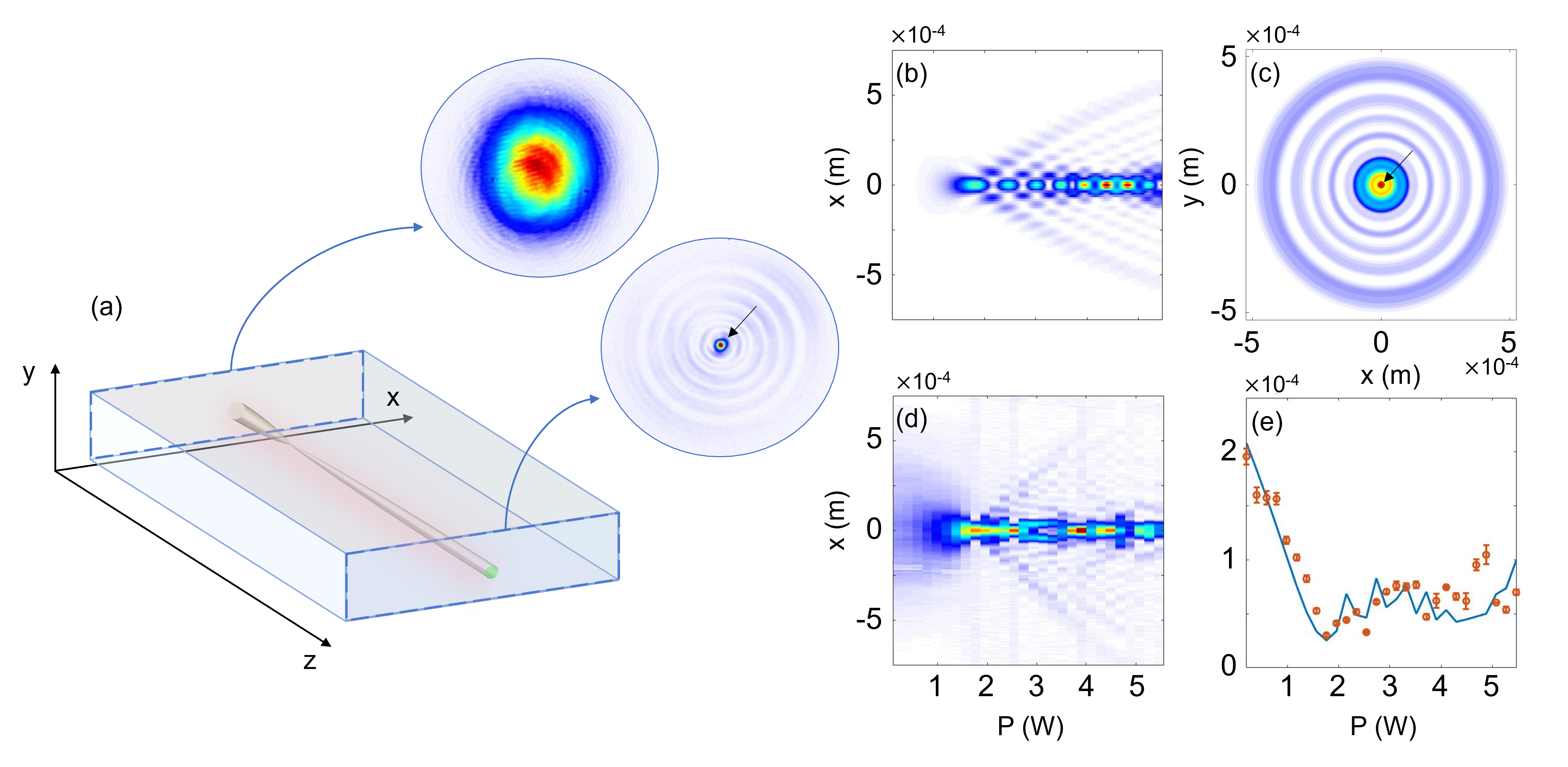
Figure 1: (a) Sketch of the experiment: a Gaussian laser beam propagating in a lead-doped crystal. The diffusion of heat inside the nonlinear medium is represented by the glowing red profile. Insets show the input and output experimental profiles at $P=5$ W. (b),(d) $y=0$ slice of the beam intensity profile as a function of one transverse coordinate $x$ and power, obtained from the numerical simulation (b) and experimental data (d). (c) Simulation of the transverse plane $(x,y)$ at $z=L$ for the power $P=5$ W. We observe the soliton (red dot indicated by the black arrow) surrounded by the classical part corresponding to $\chi\to 0$. (e) Comparison between experiment (red dots with error-bars) and simulation (blue curve) of the average size of the beam profile as a function of power.

The beam width $s=350\leavevmode\nobreak\ \mu$m at the sample input facet is chosen experimentally by a system of lenses (not shown) such that the condition $\chi\ll 1$ is fulfilled (see details in Methods). When the intense laser beam propagates inside the crystal, it induces a nonlocal interaction (heating) of the medium (depicted as a red glow around the propagating beam in Fig. 1(a)). The beam at the output facet of the medium is imaged onto a camera, where we collect its interference with a reference beam (not shown). By using the Off-Axis Digital Holography (OADH) technique [31], we are able to access the the spatial distribution of both the intensity and the phase of output field. To explore the full dynamics of the laser beam, we tune the initial power from 0.2 W to 5.5 W. The insets in Fig. 1(a) show the experimental beam intensity profile at the input and output crystal facets for input power $P=5$ W. The output intensity profile shows the expected central soliton (ground state, indicated in the figure), surrounded by the classical solution.
Experimentally, it is only possible to access the field at the output facet of the sample and not at the full nonlinear propagation inside the material. However, by expressing the propagation coordinate in terms of the relevant dynamical characteristic scale $z_{\mathrm{dyn}}=s\sqrt{n_{b}\kappa/\alpha\beta P}$ (see Methods), one can show that varying the initial power $P$ and measuring the intensity at fixed $z=L$ as a function of $L/z_{\mathrm{dyn}}$ is equivalent to measuring the intensity at different steps $z$ inside the material at fixed $P$ as a function of $z/z_{\mathrm{dyn}}$ (now with $z_{\mathrm{dyn}}$ fixed). There is hence a direct mapping between power $P$ and propagation length $z$, when $\chi\ll 1$. Tuning the power, $P$, we are able to follow the $z$-evolution of the beam amplitude $\mathcal{E}$ corresponding to the time-evolution of the mass distribution in astrophysics. We therefore hereafer use $P$ to parameterize the system evolution [see Figs. 1(b-e)].

Collapse and quasi-stationary state of the system. Figure 1(b) and (d) depict the intensity profiles (along $y=0$) measured at the output of the glass sample as a function of power $P$ obtained from the numerical simulations (details in Supplementary Discussion) and experiments, respectively. We observe good qualitative agreement of two main features, i.e., the initial collapse that is then followed by a stabilization showing that for large $P$, the system is reaching a quasi-stationary state. A plot of the simulated intensity distribution for the power $P=5$ W is shown in Fig. 1(c). It illustrates the typical expected solution which combines a solitonic part (the high intensity peak in the center of the structure) with a surrounding classical part (compare to the experimental inset in Panel (a)). A quantitative comparison is provided in Fig. 1(d) by plotting the average size of the beam $R$ (see Methods) for both the numerical simulation (curve) and experiments (circles). We observe a good agreement and the small differences in the oscillatory part after the collapse can be expected due to their chaotic nature [32], which therefore strongly depend on the experimental input conditions.

Phase-space mixing. We next study the existence of mixing in the system by analysing the evolution of the phase-space. To this end, we use the Wigner distribution (see Methods) of the full complex-valued optical field. The experimental and numerical results are presented in Fig. 2 and, here again, are in a good agreement. At the initial stage, the system has a Gaussian spatial distribution with a very narrow dispersion along the $k_{x}$-axis. As $P$ increases, the phase mixing starts by first rolling up the phase-space (indicated by the white arrows) and then forming characteristic filaments [1]. In the Supplementary Discussion, we show numerically that in a system where only mixing is present, such as in the Snyder-Mitchell model [33], the evolution of the system is significantly different. In the following, we demonstrate an additional and direct signature of violent relaxation by studying the evolution of the distribution of energy density of the system.

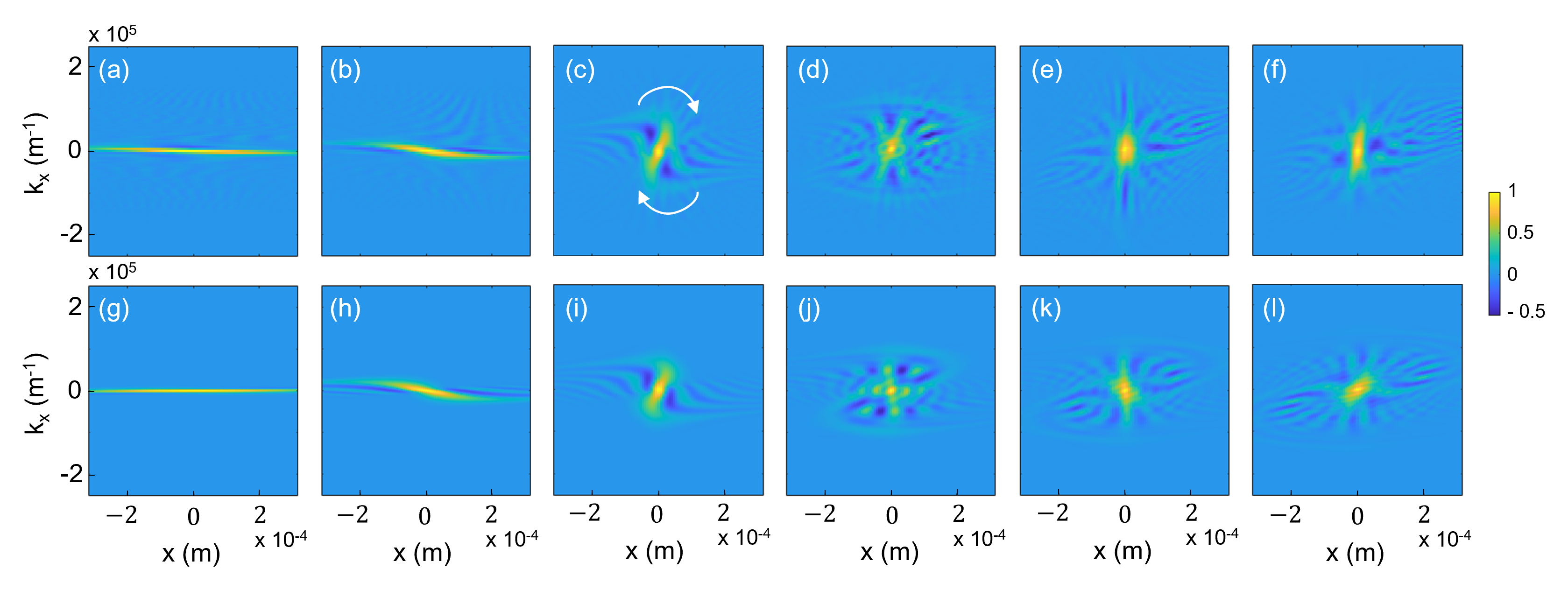
Figure 2: Results of experiment - top row (a)-(f) - and simulation - bottom row (g)-(l) - for the $y=0,k_{y}=0$ profiles of the Wigner distribution at different powers: (a),(g) $P=0.2$W, (b),(h) $P=1$W,(c),(i) $P=2$W,(d),(j) $P=3$W,(e),(k) $P=4$W,(f),(l) $P=5$W.

Direct observation of violent relaxation. In a classical system (i.e., $\chi\to 0$) with no losses, the only mechanism responsible for a change in the distribution of energy density is the violent relaxation process [1]. Figure 3 shows the experimental (a) and numerical (b) distribution of energy density, $\nu(\mathcal{E})$, obtained for various input powers, $P$. Before the minimum collapse (around $P\approx 1.8$ W), we observe that the distribution of energy density globally decreases because it is dominated by the potential energy and the system is collapsing. In contrast, after the collapse, the distribution of energy density exhibits two characteristic ‘structures’, which persist for the whole subsequent evolution: one at smaller energies, which corresponds to the inner region which has already completely relaxed. A second ‘structure’ at higher energies is related to the more peripheral regions, which have not completely relaxed yet. We observe however, as power increases after the collapse, the distribution of energy density tends asymptotically to a quasi-stationary state. At higher powers ($>5$ W) we observe (more clearly in the simulations) also the formation of a soliton that is associated with the minimal energy of the system.

Discussion. These results highlight the details of the violent relaxation dynamics. These do rely on the condition $\chi\ll 1$, so as to isolate the classical dynamics that we are interested in here. In our experiments, $\chi=2.3\times 10^{-2}/\sqrt{P}$, with $P$ measured in Watts (see Methods) and is therefore of order $10^{-2}\ll 1$ over the full evolution. However, at the same time the effect of the finite value of $\chi$ is actually still visible in the Wigner distribution (Fig. 2) where the negative regions correspond to quantum effects (see e.g. [34]). Equation (2) gives the Heisenberg uncertainty relation $\Delta k_{x}\Delta x\sim 1$, which corresponds to the typical size of the observed negative regions. These can be seen to be relatively small compared to the total surface in which the Wigner function is non-zero, indeed as a direct consequence of $\chi\ll 1$. Moreover, it is possible to explicitly show that $\chi$ is also sufficiently small as to have negligible effects also on the distribution of energy density (Supplementary Discussion).
We also note that the experimental system intrinsically exhibits losses (required to induce the nonlocal interaction through weak absorption of the beam). The total loss (including also air-glass interface reflections) is estimated to be $\sim 50\%$. These losses modify the second term of Eq. (3). However, we verified through numerical simulations (see Supplementary Discussion), that the presence of losses in the experiment has a limited impact on the distribution of energy density. Furthermore, the field evolution is only weakly modified. Drawing a connection with astrophysics, absorption and losses would correspond to a loss of mass in the system that does not alter the global dynamics and the presence of violent relaxation.

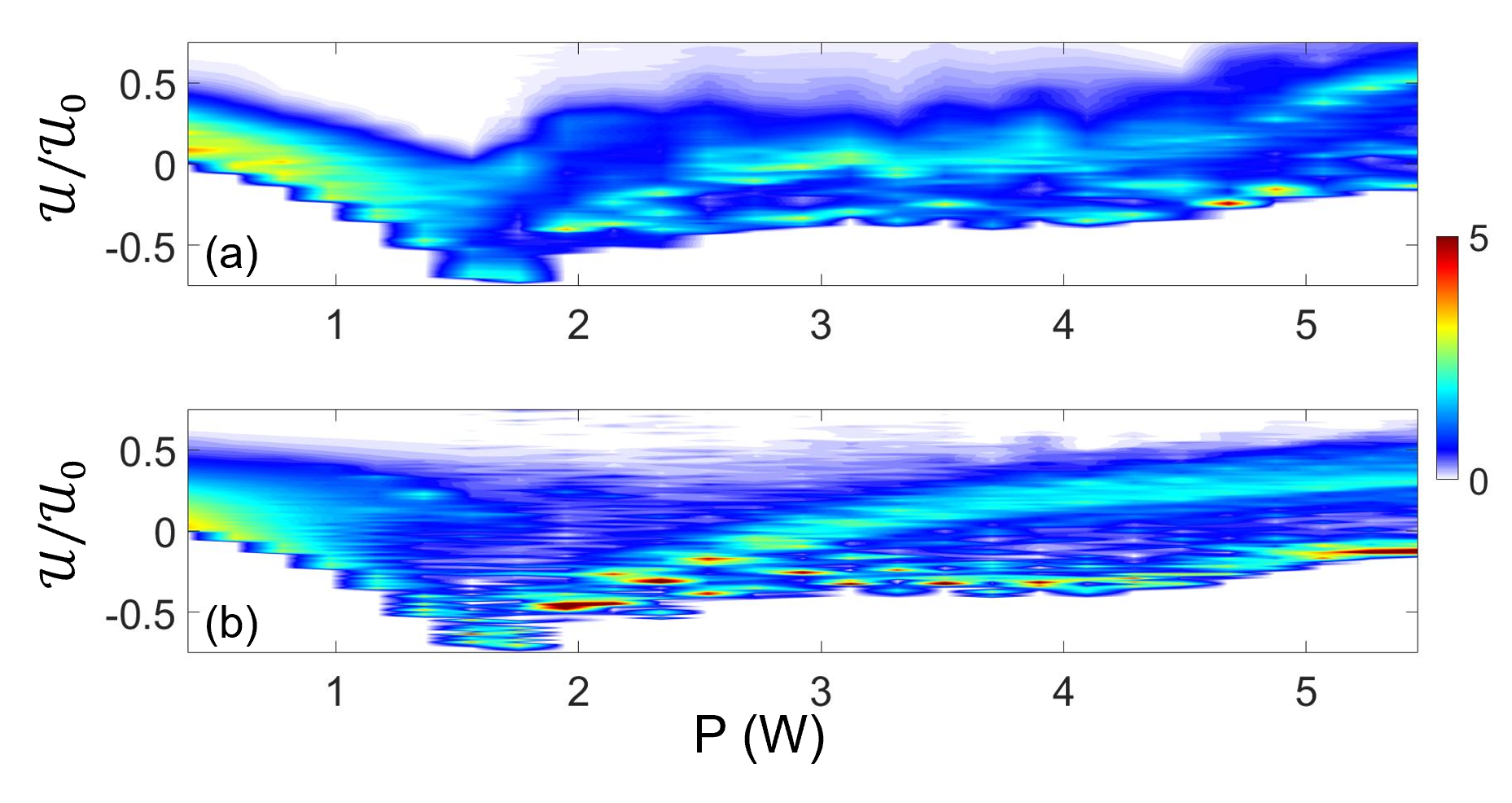
Figure 3: Distribution of energy density map a for the experiment (a) and simulation (b).

Conclusions. We have provided experimental evidence of violent relaxation in a long interaction-range system that gives a direct confirmation of the formation of an out-of-equilibrium stationary state that follows the scenario advanced by Lynden-Bell in 1967 [4]. Our experiments relate to observable galaxies whose formation dynamics are not directly observable or at least, are not repeatable. With our table-top experiments, we can directly connect our parameters to those of a particle-based system, as shown in Fig. 4, corresponding to the galaxy distribution for a particle system with parameters equivalent to those of the experiment, to be compared with Fig. 1(c), corresponding to numerics (see also SM). The parameters can then also be tuned in order to make the system more or less classical, i.e., to tune up to which spatial scale quantum effects are important. Here, we focused on the classical evolution, where the spatial scale of analogue quantum effects is one order of magnitude smaller than the size of the system.

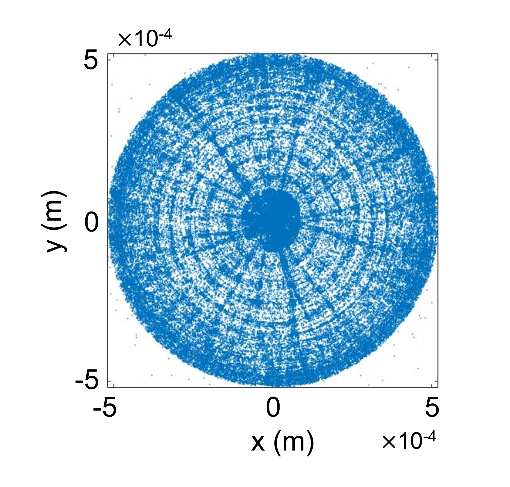
Figure 4: N-body simulation performed evolving self-gravitating particles of dark matter. We have used $2^{17}$ N-body particles and the parameters map directly on to those used in the experiments (see SM for details), i.e. this galaxy is the particle version of the optical galaxies shown in Fig. 1(a) inset (experiment) and (c) (numerical simulation).

The next steps may cover further aspects of long range systems such as investigating the effect of angular momentum, studying mergers of structures (which are known as the main mechanism of the formation of spiral galaxies), and simulating systems corresponding to various Dark Matter models.

I Methods

Experiment — The experimental setup is shown in Fig.5. A continuous-wave laser with a Gaussian profile with wavelength $\lambda=532$ nm is split into 2 components: a reference beam and a target beam. The reference beam is expanded using a system of lenses and incident onto a CMOS camera. The target beam is shaped to have waist $s=350\leavevmode\nobreak\ \mu$m (waist calculated where the intensity falls of $1/e^{2}$ - the value has been obtained by a Gaussian fit of the beam intensity at the sample input face - see inset in Fig. 1) and shines onto three aligned identical slabs of lead-doped glass (height $D=5$ mm, width $W=40$ mm and length $L_{0}=100$ mm each, hence a total length $L=300$ mm), represented as a single crystal.
The glass is a self-focusing nonlinear optical medium with thermal conductivity $\kappa=0.7$ Wm^-1K^-1, background refractive index $n_{b}=1.8$, absorption coefficient $\alpha=1m^{-1}$, thermo-optic coefficient $\beta=\frac{\partial n}{\partial T}=2.2\cdot 10^{-5}$ K^-1 and transmission coefficient at the sample interface $T=0.92$. The value of the coefficient $\beta$ is found by a fit of the experimental beam evolution and results to be 1.6 times larger than the value provided by the manufacturer. With these experimental parameters, we have $z_{\mathrm{nl}}\approx 2.7/P$ mm and $\chi=2.3\times 10^{-2}/\sqrt{P}$. As explained in the main text, since it is only possible to measure $\mathcal{E}$ at the end of the sample, in order to explore its value inside the sample we make use of mapping between propagation distance $z$ and power. This mapping holds if the parameter $\chi$ is kept constant and therefore it is necessary to vary the width $s$ of the initial condition (see the definition of $z_{dyn}$ and $\chi$ in the main paper). However, as shown in the Supplementary Discussion, for sufficiently small values of $\chi$, which is the case in our setup, the experiment is weakly sensitive to a variation of $\chi$. Therefore, we keep $s$ constant when varying $P$ to simplify the experimental procedure.

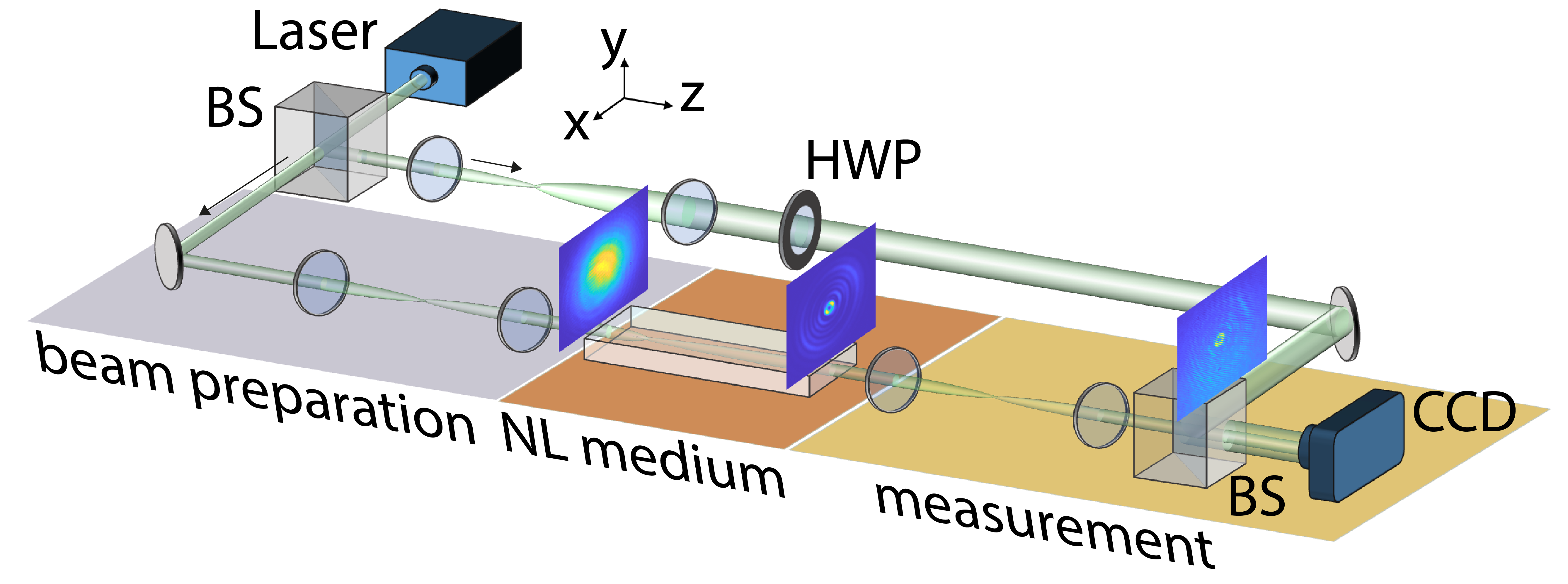
Figure 5: Experimental setup: a monochromatic laser beam is split into 2 components: a target and a reference beam. The reference beam is expanded using a system of lenses and incident onto a CMOS camera. The target beam is imaged onto the front face of the nonlinear sample through a 4f-imaging system that also allow to choose the input beam waist size. After the nonlinear propagation, the target beam at the output sample face is imaged onto a CMOS camera, where we collect its interference with the reference beam (all beams have the same optical frequency $\lambda=532$ nm). Half-wave plates ($HWP\lambda/2$) are placed along the beams paths in order to finely tune the beam polarizations in order to have the maximum visibility of the interference fringes. We collect with the CMOS camera the interferograms of the mixed field and the reference. By means of the off-axis digital holography technique [31], we are able to reconstruct the amplitudes and phases of the target beam. Target beam input powers range from $0.2\,W$ to $5.5\,W$, with a $0.25\,W$ step. Top images in the set-up sketch show the experimental intensity profile of the beam at that point in propagation distance: first image from the left is the input beam intensity, then there is the output facet beam profile ($P=5$ W); last image is the interference of the output target with the reference beam.

Data analysis — The experimental intensity profiles are characterized by a background noise - this is removed by averaging out the intensity at pixels that are at the edge of the $(x,y)$ beam profiles; this average is used as an estimate for the background noise and then subtracted from the whole experimental data. We then apply a noise mask, i.e. the intensity points far from the main body of the beam profile are set to zero. On the other hand, the interferograms do not need the noise removal, since the off axis digital holography technique requires a Fourier-transform of the beam which automatically filters all high-frequency contributions from the signal.
z to P mapping — A natural dynamical characteristic length scale $z_{\mathrm{dyn}}$ appears in the regime $\chi\ll 1$. This can be calculated writing the corresponding Newton equation of Eq. (2): $n_{b}k_{0}d^{2}\vec{r}_{\perp}/dz^{2}=k_{0}\nabla_{\perp}\Delta n$, where $\vec{r}_{\perp}$ is the position in the transverse plane. Using that the typical size $r_{\perp}\propto s$ and hence $\nabla_{\perp}\/\Delta n\propto\Delta n/s$ and the initial velocities $d\vec{r}_{\perp}/dz\simeq 0$, we get $z_{\mathrm{dyn}}=s\sqrt{n_{b}\kappa/\alpha\beta P}$. This expression allows to map $P$ with $z$.
Observables — The size of the system is measured using the quantity $R(z)=(P_{y_{0}})^{-1}\int I(x,y=0,z)\left|x\right|dx$ with $P_{y_{0}}=\int I(x,y=0,z)dx$.

Using the polar symmetry of the beam amplitude, we compute the Wigner transform [30] on the $(x,k_{x})$ plane as

$$F(x,k_{x},z)=\int dx^{\prime}\,\mathcal{E}\left(x+x^{\prime}/2,0,z\right)\mathcal{E}^{*}\left(x-x^{\prime}/2,0,z\right)e^{ik_{x}x^{\prime}},$$ (4)

where $F(x,k_{x},z)$ is a representation of the classical density of probability to find a piece of beam at the position $(x,0)$ with wavevector $(k_{x},0)$. The distribution of energy density is defined as

$$\nu(\mathcal{U})=\frac{1}{P}\int d^{2}r\,\delta\left[\mathcal{U}-\mathcal{U}(\mathbf{r},z)\right]I(\mathbf{r},z),$$ (5)

where $\delta$ is the Dirac delta function.

Acknowledgements. The authors acknowledge financial support from EPSRC (UK Grant No. EP/P006078/2) and the European Union’s Horizon 2020 research and innovation program, Grant Agreement No. 820392. D.F. acknowledges financial support from the Royal Academy of Engineering Chair in Emerging Technology programme. M.L. and B.M. acknowledges support by the grant Segal ANR-19-CE31-0017 of the French Agence Nationale de la Recherche.

Author contributions. B.M. and D.F. conceived the project and ideas. M.L., M.C.B. and R.P. performed the experiments, data analysis and numerical simulations. B.M. and E.M.W. performed theoretical analysis. D.C. contributed to numerical simulations. C.M. and M.B. contributed to data analysis. All authors contributed to the manuscript.

References

- [1] J. Binney and S. Tremaine, Galactic Dynamics: Second Edition. Princeton University Press, 2008.
- [2] I. S. Chandrasekhar, “The time of relaxation of stellar systems,” Astr. J., vol. 93, p. 285, 1941.
- [3] B. Anguiano, S. R. Majewski, C. R. Hayes, C. A. Prieto, X. Cheng, C. M. Bidin, R. L. Beaton, T. C. Beers, and D. Minniti, “The stellar velocity distribution function in the milky way galaxy,” The Astronomical Journal, vol. 160, p. 43, jun 2020.
- [4] D. Lynden-Bell, “Statistical mechanics of violent relaxation in stellar systems,” Monthly Notices of the Royal Astronomical Society, vol. 136, p. 101, 1967.
- [5] A. Campa, T. Dauxois, and S. Ruffo, “Statistical mechanics and dynamics of solvable models with long-range interactions,” Physics Reports, vol. 480, no. 3, pp. 57–159, 2009.
- [6] L. D. Landau, “On the vibrations of the electronic plasma,” J. Phys. (USSR), vol. 10, pp. 25–34, 1946.
- [7] J. Malmberg and C. Wharton, “Collisionless damping of electrostatic plasma waves,” Physical Review Letters, vol. 13, no. 6, p. 184, 1964.
- [8] V. K. Neil and A. M. Sessler, “Longitudinal resistive instabilities of intense coasting beams in particle accelerators,” Review of Scientific Instruments, vol. 36, no. 4, pp. 429–436, 1965.
- [9] L. J. Laslett, V. K. Neil, and A. M. Sessler, “Transverse resistive instabilities of intense coasting beams in particle accelerators,” Review of Scientific Instruments, vol. 36, no. 4, pp. 436–448, 1965.
- [10] C. Damm, J. Foote, A. Futch Jr, A. Hunt, K. Moses, R. Post, and J. Taylor, “Evidence for collisionless damping of unstable waves in a mirror-confined plasma,” Physical Review Letters, vol. 24, no. 10, p. 495, 1970.
- [11] K. Gentle and A. Malein, “Observations of nonlinear landau damping,” Physical Review Letters, vol. 26, no. 11, p. 625, 1971.
- [12] M. Sugawa, “Observation of self-interaction of bernstein waves by nonlinear landau damping,” Physical review letters, vol. 61, no. 5, p. 543, 1988.
- [13] J. Danielson, F. Anderegg, and C. Driscoll, “Measurement of landau damping and the evolution to a bgk equilibrium,” Physical review letters, vol. 92, no. 24, p. 245003, 2004.
- [14] C. Chen, K. Klein, and G. G. Howes, “Evidence for electron landau damping in space plasma turbulence,” Nature communications, vol. 10, no. 1, pp. 1–8, 2019.
- [15] M. Chalony, J. Barré, B. Marcos, A. Olivetti, and D. Wilkowski, “Long-range one-dimensional gravitational-like interaction in a neutral atomic cold gas,” Phys. Rev. A, vol. 87, p. 013401, Jan. 2013.
- [16] F. Zwicky, “Die Rotverschiebung von extragalaktischen Nebeln,” Helvetica Physica Acta, vol. 6, pp. 110–127, Jan. 1933.
- [17] A. Boyarsky, O. Ruchayskiy, D. Iakubovskyi, A. V. Maccio’, and D. Malyshev, “New evidence for dark matter,” arXiv e-prints, p. arXiv:0911.1774, Nov. 2009.
- [18] Y. Sofue, M. Honma, and T. Omodaka, “Unified Rotation Curve of the Galaxy – Decomposition into de Vaucouleurs Bulge, Disk, Dark Halo, and the 9-kpc Rotation Dip –,” Publications of the Astronomical Society of Japan, vol. 61, p. 227, Feb. 2009.
- [19] G. Cupani, M. Mezzetti, and F. Mardirossian, “Cluster mass estimation through fair galaxies,” Monthly Notices of the Royal Astronomical Society, vol. 403, pp. 838–847, Apr. 2010.
- [20] W. Hu, R. Barkana, and A. Gruzinov, “Fuzzy cold dark matter: the wave properties of ultralight particles,” Physical Review Letters, vol. 85, no. 6, p. 1158, 2000.
- [21] H.-Y. Schive, T. Chiueh, and T. Broadhurst, “Cosmic structure as the quantum interference of a coherent dark wave,” Nature Physics, vol. 10, no. 7, pp. 496–499, 2014.
- [22] L. Hui, J. P. Ostriker, S. Tremaine, and E. Witten, “Ultralight scalars as cosmological dark matter,” Physical Review D, vol. 95, no. 4, p. 043541, 2017.
- [23] D. J. Marsh and J. C. Niemeyer, “Strong constraints on fuzzy dark matter from ultrafaint dwarf galaxy eridanus ii,” Physical review letters, vol. 123, no. 5, p. 051103, 2019.
- [24] S. Alexander, J. J. Bramburger, and E. McDonough, “Dark disk substructure and superfluid dark matter,” Physics Letters B, vol. 797, p. 134871, 2019.
- [25] I. M. Moroz, R. Penrose, and P. Tod, “Spherically-symmetric solutions of the Schrödinger-Newton equations,” Classical and Quantum Gravity, vol. 15, pp. 2733–2742, Sept. 1998.
- [26] P. Mocz, L. Lancaster, A. Fialkov, F. Becerra, and P.-H. Chavanis, “Schrödinger-poisson–vlasov-poisson correspondence,” Physical Review D, vol. 97, no. 8, p. 083519, 2018.
- [27] T. Roger, C. Maitland, K. Wilson, N. Westerberg, D. Vocke, E. M. Wright, and D. Faccio, “Optical analogues of the newton–schrödinger equation and boson star evolution,” Nature communications, vol. 7, no. 1, pp. 1–8, 2016.
- [28] R. Bekenstein, R. Schley, M. Mutzafi, C. Rotschild, and M. Segev, “Optical simulations of gravitational effects in the newton–schrödinger system,” Nature Physics, vol. 11, no. 10, pp. 872–878, 2015.
- [29] A. Navarrete, A. Paredes, J. R. Salgueiro, and H. Michinel, “Spatial solitons in thermo-optical media from the nonlinear schrödinger-poisson equation and dark-matter analogs,” Physical Review A, vol. 95, no. 1, p. 013844, 2017.
- [30] E. P. Wigner, “On the quantum correction for thermodynamic equilibrium,” in Part I: Physical Chemistry. Part II: Solid State Physics, pp. 110–120, Springer, 1997.
- [31] J. Bertolotti, “Off-Axis Digital Holography Tutorial.” https://jacopobertolotti.com/tutorials.html.
- [32] P. O. Vandervoort, “On chaos in the oscillations of galaxies,” Monthly Notices of the Royal Astronomical Society, vol. 411, pp. 37–53, 01 2011.
- [33] A. W. Snyder and D. J. Mitchell, “Accessible solitons,” Science, vol. 276, no. 5318, pp. 1538–1541, 1997.
- [34] E. J. Heller, “Phase space interpretation of semiclassical theory,” The Journal of Chemical Physics, vol. 67, no. 7, pp. 3339–3351, 1977.