RSI-Grad-CAM: Visual Explanations from Deep Networks via Riemann-Stieltjes Integrated Gradient-based Localization

Neural networks are becoming increasingly better at tasks that involve classifying and recognizing images. At the same time techniques intended to explain the network output have been proposed. One such technique is the Gradient-based Class Activation Map (Grad-CAM), which is able to locate features of an input image at various levels of a convolutional neural network (CNN), but is sensitive to the vanishing gradients problem. There are techniques such as Integrated Gradients (IG), that are not affected by that problem, but its use is limited to the input layer of a network. Here we introduce a new technique to produce visual explanations for the predictions of a CNN. Like Grad-CAM, our method can be applied to any layer of the network, and like Integrated Gradients it is not affected by the problem of vanishing gradients. For efficiency, gradient integration is performed numerically at the layer level using a Riemann-Stieltjes sum approximation. Compared to Grad-CAM, heatmaps produced by our algorithm are better focused in the areas of interest, and their numerical computation is more stable. Our code is available at https://github.com/mlerma54/RSIGradCAM.

1 Introduction

The visualization of features captured by convolutional neural networks (CNN) helps explain how they make their predictions. This is a field of rapid development in which many techniques have been proposed, tested, and validated; methods to provide explanations for the predictions of a CNN can be grouped into three main categories: primary attribution methods, layer attribution methods and neuron attribution methods [Hochreiter 2020].

Primary attribution methods evaluate the contribution of each input to the output of a model. This approach is model-agnostic, meaning that primary attribution methods work the same regardless of the internal structure of the network or machine learning system used, in that depends only on inputs and outputs, not on internal structure. Some examples are Integrated Gradients (IG) [Sundararajan 2017] and Local Interpretable Model-Agnostic Explanations (LIME) [Ribeiro 2016].

Layer attribution methods evaluate the contribution of each neuron in a given layer to the output of the model. These methods are useful to determine the location of medium and high level features such as the spacial location of the various elements that compose an image. Some examples are Class Activation Mapping (CAM) [Zhou 2016] and its derivatives such as Gradient-based CAM (Grad-CAM) [Selvaraju 2017] and Grad-CAM++ [Chattopadhyay 2018].

Neuron attribution methods evaluate the contribution of each input feature to the activation of given hidden neurons. Both primary and layer attribution methods can be converted into neuron attribution methods by replacing the network output with any neuron activation. For instance Neuron Integrated Gradients is equivalent to Integrated Gradients considering the output to be simply the output of the identified neuron. They may be useful when we are interested in determining how the activation of a given neuron, rather than the network output, depends on the input of the network. It is also possible to combine the effect of the input on a given neuron and the effect of the neuron on the network output, as in the Neuron Conductance method described in [Dhamdhere 2018].

In our study we look at three gradient based methods: Gradient Guided Class Activation Map (Grad-CAM, a layer attribution method) [Selvaraju 2017], Integrated Gradients (a primary attribution method) [Sundararajan 2017], and Integrated Grad-CAM (layer attribution) [Sattarzadeh 2021]. We examine their advantages and limitations, and propose a modification of Grad-CAM in which gradients are replaced with integration of gradients computed at any layer rather than the input layer. This allows our method to simultaneously overcome the limitations of grad-CAM, and Integrated Gradients, namely vulnerability to the vanishing gradients problem, and applicability to the network input only respectively.

2 Previous Work

Our attribution method combines ideas from two existing techniques: Grad-CAM and Integrated Gradients. In this section we explain how these methods work. We also look at the Integrated Grad-CAM technique introduced in [Sattarzadeh 2021], and show how it differs from ours.

2.1 Grad-CAM

The technique introduced in [Selvaraju 2017] uses the gradients of any target concept flowing into a convolutional layer to produce a heatmap, also called saliency map or localization map, intended to highlight the contribution of regions in the image for predicting the concept.

Grad-CAM works as follows (see Figure 1). First we must pick a convolutional layer $A$, which is composed of a number of feature maps, also called channels, $A^{1},A^{2},\dots,A^{N}$ (where $N$ is the number of feature maps in the picked layer), all of them with the same dimensions. At the network input they are just the three RGB channels of the input image. In the following layers the channels/feature maps are supposed to capture progressively higher features of the image (beginning with edge detection, shapes, textures, geometric shapes, and ultimately whole categories such as “dog” and “cat”). We will use the term “channels” when referring to the third dimension of a layer, and “feature maps” if we want to stress their feature capturing role.

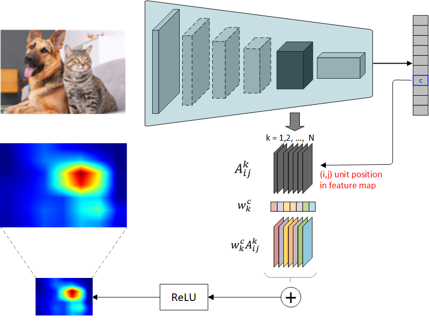
Figure 1: Grad-CAM overview

Let $A^{k}$ be the $k$-th feature map of the picked layer, and let $A_{ij}^{k}$ be the activation of the unit in the position $(i,j)$ of the $k$-th feature map. Then, the localization map, or “heatmap,” is obtained by combining the feature maps of the layer using weights $w_{k}^{c}$ that capture the contribution of the $k$-th feature map to the output $y^{c}$ of the network corresponding to class $c$.

In order to compute the weights, we pick a class $c$ and determine how much the output $y^{c}$ of the network depends of each unit of the $k$-th feature map, as measured by the gradient $\partial y^{c}/\partial A_{ij}^{k}$, which can be obtained by using the backpropagation algorithm. The gradients are then averaged thorough the feature map to yield a weight $w_{k}^{c}$, as indicated in equation (1). Here $Z$ is the size (number of units) of the feature map.

$$w_{k}^{c}=\overbrace{\frac{1}{Z}\sum_{i}\sum_{j}}^{\text{global average pooling}}\hskip-30.0pt\underbrace{\frac{\partial y^{c}}{\partial A_{ij}^{k}}}_{\text{gradients via backprop}}$$ (1)

Optionally, the weights could be computed using positive gradients:

$$w_{k}^{c}=\frac{1}{Z}\sum_{i}\sum_{j}\text{ReLU}\left(\frac{\partial y^{c}}{\partial A_{ij}^{k}}\right)$$ (2)

Where $\text{ReLU}(x)=\text{max}(x,0)$ is the Rectified Linear Unit function. This can be justified by the intuition that negative gradients correspond to units where features from a class different from the chosen class are present.

The next step consists of combining the feature maps $A^{k}$ with the weights computed above, as shown in equation (3). Note that the combination is also followed by a Rectified Linear Unit function $\text{ReLU}(x)=\text{max}(x,0)$, because we are interested only in the features that have a positive influence on the class of interest. The result $L_{\text{Grad-CAM}}^{c}$ is called class-discriminative localization map by the authors. It can be interpreted as a coarse heatmap of the same size as the chosen convolutional feature map.

$$L_{\text{Grad-CAM}}^{c}=\text{ReLU}\underbrace{\Biggl{(}\sum_{k}w_{k}^{c}A^{k}\Biggr{)}}_{\text{linear combination}}$$ (3)

After the heatmap has been produced, it can be normalized and upsampled via bilinear interpolation to the size of the original image, and overlapped with it to highlight the areas of the input image that contribute to the network output corresponding to the chosen class (see Figure 2).

Figure 2: Original image (left). Grad-CAM locating a dog (center) and a cat (right).

The method is very general, and can be applied to any (differentiable) network outputs.

In spite of its success, Grad-CAM has a limitation. It has the possibility of getting a very small or practically zero gradient ($\partial y^{c}/\partial A_{ij}^{k}\approx 0)$ when the network output is near saturation, i.e., when the value of the output is very close to its maximum (say $100\%$ score assigned to a class). In this instance, any increase in the value is very small (almost zero). This vanishing gradient problem was first noticed in the context of training neural networks by the backpropagation algorithm (see e.g. [Hochreiter 1998]), but it can appear in any application based on backpropagating gradients. If the saturation occurs at the network output, then it can be palliated by replacing the final output of the network (typically a softmax) with the activations of the layer right before the final softmax (as in the description included in [Selvaraju 2017]), however the problem can potentially affect any layer.

2.2 Integrated Gradients

A related attribution technique, introduced in [Sundararajan 2017], is Integrated Gradients (IG). The authors study the problem of finding a method to attribute predictions of a deep network to its input features that verifies two desirable properties (called “axioms” by the authors). To formulate them we need a baseline input in which all features are absent (e.g. a blank image), and a given input in which some features are present (say the image of a fireboat). The properties are the following:

• Sensitivity: For every input and baseline that differ in one feature but have different predictions, the differing feature should be given a non-zero attribution.

• Implementation invariance: Two functionally equivalent networks should have identical attributions for the same input image and baseline image.

The sensitivity property is violated by Grad-CAM and other methods relying on gradients. This happens because a relevant feature may be given no attribution due to vanishing gradient when the network output gets close to its saturation point. The authors present this example: consider a one variable, one ReLU network implementing the following function:

$$f(x)=1-\text{ReLU}(1-x)$$ (4)

Its graph is shown in Figure 3.

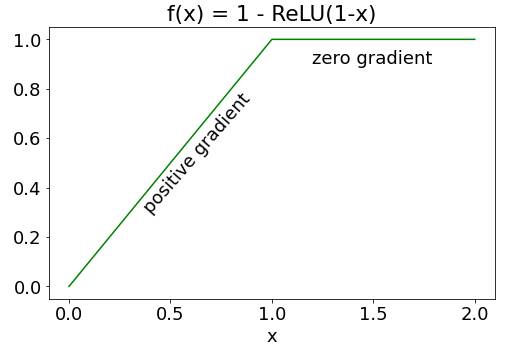
Figure 3: Example of violation of the sensitivity property because of vanishing gradient.

Suppose the input is $x=2$ and its associated baseline is $x=0$. Then, the function changes from $f(0)=0$ to $f(2)=1$, but $f(x)$ becomes flat for $x>1$, and the gradient method gives attribution $f^{\prime}(2)=0$. But this contradicts the fact that the value of the function has changed, so the attribution should not be zero.

The method proposed in [Sundararajan 2017] is immune to that problem because it does not depend only on one gradient at a given level of activation, but on the result of integrating gradients along a set of network inputs obtained by interpolating between a baseline input (e.g. a black image) and the actual desired input.

The authors describe their method with a theoretical model that uses continuous functions, and later describe how to implement it in a discrete setting. They interpret a network as a multivariate function $F:\mathbb{R}^{d}\to[0,1]$ from its $d$ inputs to the prediction $F(x)$ of the network for a given input $x\in\mathbb{R}^{d}$. In case $x$ represents an image, then $d$ would be its number of pixels, and $F(x)$ may represent the probability that the image contains a given object, say a fireboat. The goal would be to determine which pixels in the image contribute to the prediction of the network, in other words, which of those pixels are part of the fireboat image.

Hence, instead of using a single image the method uses a sequence of interpolated images between a baseline $x^{\prime}$ and the given image $x$:

$$\gamma(\alpha)=x^{\prime}+\alpha(x-x^{\prime})\qquad 0\leq\alpha\leq 1$$ (5)

Each interpolated image is a combination of $\gamma(0)=x^{\prime}$ (baseline) and $\gamma(1)=x$ (given image). Then, the gradient of the network output with respect to each input pixel $x_{i}$ is integrated as shown in equation (6).

$$\texttt{IntegratedGrads}_{i}(x)::=\\ (x_{i}-x^{\prime}_{i})\times\int_{\alpha=0}^{1}\frac{\partial F(x^{\prime}+\alpha\times(x-x^{\prime}))}{\partial x_{i}}\,d\alpha$$ (6)

In the equation, the factor $(x-x^{\prime})$ appears when using as variables of integration the pixel values of the interpolated image, so that the differential within the integral is $d(x^{\prime}+\alpha\times(x-x^{\prime}))=(x-x^{\prime})\times d\alpha$. Since it does not depend on $\alpha$, the factor $(x-x^{\prime})$ can be taken outside the integral.

In practice the integral can be approximated numerically with a Riemann sum:

$$\texttt{IntegratedGrads}_{i}^{approx}(x)::=\\ (x_{i}-x^{\prime}_{i})\sum_{\ell=1}^{m}\frac{\partial F(x^{\prime}+\frac{\ell}{m}\times(x-x^{\prime}))}{\partial x_{i}}\times\frac{1}{m}$$ (7)

where $m$ represents the number of interpolation steps. This parameter $m$ can be adjusted by experimentation, although it is recommended to give it a value between 50 and 200.

The result plays the role of a localization map, although compared to Grad-CAM, Integrated Gradients tends to look more grainy, while Grad-CAM heatmaps are smoother (see Figure 4 as an example).

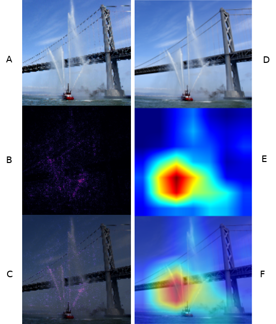
Figure 4: A fireboat image located by Integrated Gradients (left) and Grad-CAM (right). For integrated gradients it is shown: (A) input image, (B) IG attribution mask, (C) overlay of attribution mask with original image. For Grad-CAM we show (D) the original image, (E) heatmap, (F) overlay.

The IG attribution mask is the output of Integrated Gradients for this figure, showing the contribution of each input pixel to the class “fireboat.”

A problem with the Integrated Gradients method is that it is designed for working with the network inputs and may miss features captured at hidden layers. A workaround consists of considering the activations of a hidden layer $A$ as input of the part of the network above that layer, as suggested in the layer integrated gradients method listed in [Hochreiter 2020]. The role of the inputs now will be played by the activations of layer $A$, and the value of $F$ will be the output of the network $y^{c}$ for some fix class $c$. Let $A_{\text{baseline}}$ be the activations of layer $A$ when we feed the network with the baseline input $x^{\prime}$, and let $A_{\text{final}}$ be the activations of layer $A$ when the we feed the network with the final input $x$. Then a linear interpolation at the layer level yields

$$A(\alpha)=A_{\text{baseline}}+\alpha\,(A_{\text{final}}-A_{\text{baseline}})\qquad 0\leq\alpha\leq 1$$ (8)

Let $y^{c}(\alpha)$ be the network output for a value of $\alpha$ between 0 and 1. Using equation (7) we get a localization map $L$ with the same shape as $A$ and elements

$$L_{ij}^{k}=(A_{ij}^{k}(1)-A_{ij}^{k}(0))\left(\frac{1}{m}\sum_{\ell=1}^{m}\frac{\partial y^{c}(\alpha_{\ell})}{\partial A_{ij}^{k}}\right)$$ (9)

The result can be expressed in a more compact way as follows:

$$L=(A(1)-A(0))\odot\left(\frac{1}{m}\sum_{\ell=1}^{m}\frac{\partial y^{c}(\alpha_{\ell})}{\partial A}\right)$$ (10)

where $\odot$ represents the Hadamard (element-wise) product [Horn 2012]. For visualization purposes $L$ can be summed across its channels, i.e., $L^{\prime}=\sum_{k=1}^{N}L^{k}$, max-min normalized, and finally resized to the size of the original image.

We note that the axiomatic properties of IG applied to a hidden layer may still hold for the part of the network above the chosen layer, but it won’t hold for the whole network—in particular the method won’t be implementation invariant anymore. Another issue concerns the choice of baseline for a hidden layer. While such choice can be guided by heuristic arguments when dealing with network inputs such as images, it is less clear when dealing with latent features at the layer level—what set of activations can be taken to mean “absence” of a feature?

2.3 Integrated Grad-CAM

Suitable combinations of the ideas behind Grad-CAM and Integrated Gradients can lead to new techniques that overcome the shortcomings of each of them, particularly:

• Violation of the sensitivity axiom by Grad-CAM.

• Applicability of Integrated Gradients to network inputs only.

Next, we will discuss the Integrated Grad-CAM technique introduced in [Sattarzadeh 2021].

Combining equations (1) and (3) we get the following expression for the final heatmap in the original Grad-CAM:

$$L_{\text{Grad-CAM}}^{c}=\text{ReLU}\Biggl{(}\sum_{k}\frac{1}{Z}\sum_{i,j}\frac{\partial y^{c}}{\partial A_{ij}^{k}}A^{k}\Biggr{)}$$ (11)

Similarly to Integrated Gradients, the authors use a set of interpolated images between a baseline $x^{\prime}$ and a final image $x$ as shown in (5). Those images are fed to the network, and for each of them the activations of the chosen layer and the gradients of the score $y^{c}$ respect to the activations $A_{ij}^{k}$ are computed. Then, an explanation map $M^{c}$ (playing the role of Grad-CAM’s $L^{c}$ localization map) is generated using the following formula:

$$M^{c}=\int_{\alpha=0}^{1}\text{ReLU}\Biggl{(}\sum_{k}\sum_{i,j}\frac{\partial y^{c}(\alpha)}{\partial A_{ij}^{k}}\Delta_{k}(\alpha)\Biggr{)}\,d\alpha$$ (12)

where $\Delta_{k}(\alpha)=A^{k}(\alpha)-A^{k}(0)$. Here $\partial y^{c}(\alpha)/\partial A_{ij}^{k}$ represents the partial derivative of $y^{c}$ with respect to $A_{ij}^{k}$ when the input $\gamma(\alpha)=x^{\prime}+\alpha(x-x^{\prime})$ is fed to the network, and $A_{ij}^{k}(\alpha)$ is the value of the activation in location $(i,j)$ of the $k$-th feature map of the chosen layer. The explanation map can be computed numerically using a Riemann sum for the integral:

$$M^{c}\approx\sum_{\ell=1}^{m}\text{ReLU}\Biggl{(}\frac{1}{m}\sum_{k}\sum_{i,j}\frac{\partial y^{c}(\alpha_{\ell})}{\partial A_{ij}^{k}}\Delta_{k}(\alpha_{\ell})\Biggr{)}$$ (13)

where $m$ is the number of interpolation steps, and $\alpha_{\ell}=\ell/m$. Finally, $M^{c}$ is upsampled to the dimensions of the input image via bilinear interpolation.

Comparing (11) and (12) we see that the Integrated Grad-CAM equations differs from Grad-CAM in the following:

• The factor $1/Z$ is missing, which is not really relevant since the heatmap obtained is typically normalized to a fix interval of intensities, hence a global constant factor can be ignored.

• The activations of the feature maps $A^{k}$ are replaced with the differences $\Delta_{k}(\alpha)=A^{k}(\alpha)-A^{k}(0)$ between activations obtained when the network is fed with an interpolated image and the ones corresponding to the baseline.

• The final explanation map is integrated along the set of interpolated images.

In sum, the method is equivalent to averaging Grad-CAM saliency maps obtained for multiple copies of the input, which are linearly interpolated with the defined baseline.

3 Methodology

In this section we will introduce a novel attribution method combining ideas from Grad-CAM and Integrated Gradients, but essentially different from the approach used in Integrated Grad-CAM. Also, our method, unlike Integrated Gradients, is not based on axioms. The authors of IG express skepticism about empirical evaluations of attribution methods, for that reason their work is based on axioms capturing desirable properties of an attribution method. Our work will rely on empirical evaluations. In the next section we will provide metrics showing how our method overperforms Grad-CAM and Integrated Grad-CAM.

Like the Integrated Gradients attribution method, our algorithm feeds the network with a set of inputs obtained by interpolation between a baseline and a final input. Then, it computes feature-map weights to be used like in Grad-CAM, except that instead of gradients it uses the integral of those gradients to compute the weight assigned to each feature-map.

The computation of the integrated gradients is formally equivalent to the numerical computation of a Riemann-Stieltjes Integral [Protter 1991]. We start with a brief explanation of the concepts and mathematical techniques, and then show how to use them to produce the three attribution methods: Grad-CAM, Integrated Grad-CAM, and our RSI-Grad-CAM. We finish with a summary comparing the methods discussed.

3.1 Motivation and Theoretical Background

Our technique aims to replace the gradients of the activations $A_{ij}^{k}$ used by Grad-CAM with their integral as the network is fed by a sequence of interpolated images (recall that $k$ indexes the feature maps within a given layer, and $(i,j)$ is the location of each of the units of the feature map). The main motivation is that we are not interested in how much the output network $y^{c}$ for a given class $c$ changes for an infinitesimal change of the activations $A_{ij}^{k}$, but how much it changes along the whole interval of values taken by each activation $A_{ij}^{k}$ as the image fed to the network goes from baseline to final image. The idea behind this technique is inspired by the gradient theorem for line integrals [Williamson 2004, p. 374]: a line integral through a gradient field $\nabla F$ of a scalar vector field $F\!:\!\mathbb{R}^{n}\to\mathbb{R}$ along a given curve $\gamma\!:\![0,1]\to\mathbb{R}^{n}$ equals the difference between the values of the scalar field at the endpoints $\mathbf{p}=\gamma(0)$ and $\mathbf{q}=\gamma(1)$ of the curve:

$$F(\mathbf{q})-F(\mathbf{p})=\\ \int_{\gamma}\nabla F(\mathbf{x})\cdot d\mathbf{r}=\int_{\gamma}\sum_{i=1}^{n}\frac{\partial F}{\partial x_{i}}dx_{i}\sum_{i=1}^{n}\int_{\gamma}\frac{\partial F}{\partial x_{i}}dx_{i}$$ (14)

Each term $\int_{\gamma}\frac{\partial F}{\partial x_{i}}dx_{i}$ of the final sum is the contribution of the $i$-th variable $x_{i}$ to the total change of $F$. The gradient theorem is the basis of the completeness property of Integrated Gradients [Sundararajan 2017, proposition 1]. In our case, the function will be the output of the network for a given class $y^{c}$, and the variables of integration will be the activations $A_{ij}^{k}$. The gradients are $\partial y^{c}/\partial A_{ij}^{k}$, and the term corresponding to the contribution of unit $(i,j)$ in feature map $k$ will be $\int_{\gamma}\frac{\partial y^{c}}{\partial A_{ij}^{k}}\,dA_{ij}^{k}$.

Note that the $A_{ij}^{k}$ are not independent variables, but (potentially complicated) functions of the network inputs. An integral in which the variable of integration is replaced with a function is called a Riemann-Stieltjes integral [Protter 1991]. In general the integral of a function $f$ with respect to another function $g$ is expressed like this:

$$\int_{a}^{b}f(x)\,dg(x)$$ (15)

where $g(x)$ is called the integrator. In our problem the activations $A_{ij}^{k}$ will play the role of integrators. This kind of integral can be numerically approximated with a modification of a Riemann sum as follows:

$$\int_{a}^{b}f(x)\,dg(x)\approx\sum_{\ell=1}^{m}f(x_{\ell})[g(x_{\ell})-g(x_{\ell-1})]$$ (16)

where $x_{\ell}=a+\tfrac{\ell}{m}(b-a)$.

3.2 Riemann-Stieltjes Sum Approximation

Here the idea is to use a Riemann-Stieltjes integral like (15), with $f=\partial y^{c}/\partial A_{ij}^{k}$ as integrand, and $g=A_{ij}^{k}$ in the role of integrator, so the weight assigned to feature-map $k$ of the chosen layer for a given class $c$ will be:

$$w_{k}^{c}=\frac{1}{Z}\sum_{i,j}\int_{\alpha=0}^{\alpha=1}\frac{\partial y^{c}(\alpha)}{\partial A_{ij}^{k}}\,dA_{ij}^{k}(\alpha)$$ (17)

where $\alpha$ is the interpolating parameter varying between $0$ and $1$.

Note that (17) is just a line integral of the gradient of $y^{c}$ as a function of the activations $A_{ij}^{k}$, along the parametric curve $A^{k}(\alpha)$ joining $A^{k}(0)$ and $A^{k}(1)$.

The approximate value of the integral in (17) is given by the following Riemann-Stieltjes sum, as in (16):

$$\int_{\alpha=0}^{\alpha=1}\frac{\partial y^{c}(\alpha)}{\partial A_{ij}^{k}}\,dA_{ij}^{k}(\alpha)\approx\\ \sum_{\ell=1}^{m}\Biggl{\{}\frac{\partial y^{c}(\alpha_{\ell})}{\partial A_{ij}^{k}}\times\Delta A_{ij}^{k}(\alpha_{\ell}))\Biggr{\}}$$ (18)

where $\alpha_{\ell}=\ell/m$ and $\Delta A_{ij}^{k}(\alpha_{\ell})=A_{ij}^{k}(\alpha_{\ell})-A_{ij}^{k}(\alpha_{\ell-1})$. Hence, the following is a numerical approximation of the $w_{k}^{c}$:

$$w_{k}^{c}=\frac{1}{Z}\sum_{i,j}\left(\sum_{\ell=1}^{m}\Biggl{\{}\frac{\partial y^{c}(\alpha_{\ell})}{\partial A_{ij}^{k}}\times\Delta A_{ij}^{k}(\alpha_{\ell})\Biggr{\}}\right)$$ (19)

As mentioned for Grad-CAM, optionally the integrated gradients can be replaced with positive integrated gradients if we want to use only the units that contribute positively to the output of the network:

$$w_{k}^{c}=\frac{1}{Z}\sum_{i,j}\text{ReLU}\left(\sum_{\ell=1}^{m}\Biggl{\{}\frac{\partial y^{c}(\alpha_{\ell})}{\partial A_{ij}^{k}}\times\Delta A_{ij}^{k}(\alpha_{\ell})\Biggr{\}}\right)$$ (20)

3.3 Summary of methods and theoretical contributions

We summarize our theoretical contributions by restating the localization maps for each method and highlight their differences. Unless otherwise stated, the localization maps will be min-max normalized and resized to the shape of the original image.

Grad-CAM. Equation (3) with weights explicitly written:

$$L^{c}_{\text{Grad-CAM}}=\\ \text{ReLU}\Biggl{\{}\sum_{k}\Bigl{(}\underbrace{\frac{1}{Z}\sum_{i}\sum_{j}\frac{\partial y^{c}}{\partial A_{ij}^{k}}}_{w_{k}}\Bigr{)}A^{k}\Biggr{\}}$$ (21)

Integrated Gradients. Equation (10):

$$L^{c}_{\text{Integrated Gradients}}\approx\\ (A(1)-A(0))\odot\left(\frac{1}{m}\sum_{\ell=1}^{m}\frac{\partial y^{c}(\alpha_{\ell})}{\partial A}\right)$$ (22)

where $\partial y^{c}(\alpha_{\ell})/\partial A$ represents the 3D tensor with elements $\partial y^{c}(\alpha_{\ell})/\partial A_{ij}^{k}$, and $\odot$ represents Hadamard (element-wise) product [Horn 2012]. Note that the result is a 3D tensor with the same shape as $A$, although a 2D localization map can be obtained by adding the tensor feature maps across its channels.

Integrated Grad-CAM. Equation (13):

$$L^{c}_{\text{Integrated Grad-CAM}}\approx\\ \frac{1}{m}\sum_{\ell=1}^{m}\text{ReLU}\Biggl{\{}\sum_{k}\Bigl{(}\underbrace{\sum_{i,j}\frac{\partial y^{c}(\alpha_{\ell})}{\partial A_{ij}^{k}}}_{w_{k}}\Bigr{)}\Delta_{k}(\alpha_{\ell})\Biggr{\}}$$ (23)

where $\Delta_{k}(\alpha_{\ell})=A^{k}(\alpha_{\ell})-A^{k}(0)$. The method is equivalent to averaging Grad-CAM localization maps obtained from a sequence of interpolated input images.

RSI-Grad-CAM. Approximate integration of gradients with Riemann-Stieltjes sum (our method), based on equation (19):

$$L^{c}_{\text{RSI-Grad-CAM}}\approx\\ \text{ReLU}\Biggl{\{}\sum_{k}\Biggl{(}\underbrace{\frac{1}{Z}\sum_{ij}\Bigl{(}\sum_{\ell=1}^{m}\frac{\partial y^{c}(\alpha_{\ell})}{\partial A_{ij}^{k}}\Delta A_{ij}^{k}(\alpha_{\ell})\Bigr{)}}_{w_{k}}\Biggr{)}A^{k}\Biggr{\}}$$ (24)

where $\Delta A_{ij}^{k}(\alpha_{\ell})=A_{ij}^{k}(\alpha_{\ell})-A_{ij}^{k}(\alpha_{\ell-1})$.

Gradients have been replaced with Riemann-Stieltjes integrated gradients (approximated with Riemann-Stieltjes sums).

3.4 Metrics

We will compare the performance of Grad-CAM, Integrated Grad-CAM and our RSI-Grad-CAM based on their numerical stability, and two quantitative evaluation approaches:

• Quantitative Evaluations Without Ground Truth.

• Quantitative Evaluations With Ground Truth.

3.4.1 Numerical stability

When computing mathematical operations we need to use a limited number of bits to express real numbers, which may lead to approximation errors. Those errors can accumulate, leading to the failure of theoretically successful algorithms. One potential problem that may impact the algorithms examined here is division by a near-zero number.

One of the steps in producing a heatmap for an attribution method is performing min-max normalization, i.e., for each pixel with coordinates $(i,j)$ we replace the heatmap pixel value $L(i,j)$ with

$$L_{norm}(i,j)=\frac{L(i,j)-\min(L)}{\max(L)-\min(L)}$$ (25)

so the normalized pixel values range from 0 to 1. Since the pixel values of a heatmap are computed using gradients, and vanishing gradients are a common problem in some architectures, the final result may involve zero or near zero pixel values in the raw (non-normalized) heatmap.

In order to avoid division by zero or near zero we will include a small term $\varepsilon$ in the bottom of the fraction used for normalization:

$$L_{norm}(i,j)=\frac{L(i,j)-\min(L)}{\max(L)-\min(L)+\varepsilon}$$ (26)

This parameter $\varepsilon$ plays the role of an hyperparameter that needs to be tweaked. If its value is too large it will distort the heatmap, if it is too low it won’t be suitable to prevent underflow errors.

The range of values taken by raw (non-normalized) heatmaps across an image dataset provides an indication of the numerical stability of an attribution method.

3.4.2 Quantitative Evaluations Without Ground Truth

We use quantitative evaluations that do not require ground truth as used in [Chattopadhyay 2018]. The idea behind these kinds of evaluations is to measure how much the prediction of the network changes when the original image is replaced by the parts of the image highlighted by the heatmap produced by the attribution method being tested.

Given an image $I$ and a heatmap $L^{c}$ generated for this image for class $c$, we find an explanation map $E^{c}=L^{c}\odot I$, where $\odot$ represents the Hadamard (element-wise) product of $L^{c}$ and $I$. Since the heatmap is a 2D array and the image has three color channels, the Hadamard product $E^{c}=L^{c}\odot I$ actually means the element-wise product of $L^{c}$ by each of the three channels of $I$, i.e., if the elements of $E^{c}$, $L^{c}$, and $I$ are respectively $e^{c}_{ijk}$, $l^{c}_{ij}$, $p_{ijk}$, then $e^{c}_{ijk}=l^{c}_{ij}\cdot p_{ijk}$.

Figure 5 shows an example of image, heatmap, and resulting explanation map.

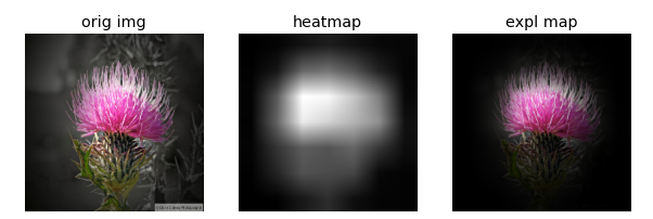
Figure 5: Original image, heatmap, and explanation map.

Feeding the network with an image $I$ we obtain an output $Y^{c}=$ predicted probability of class $c$. If we feed the network with the explanation map $E^{c}$ we will obtain an output $O^{c}$. For a good attribution method we expect $O^{c}$ to be close to the predicted probability $Y^{c}$. Based on this idea, the following metrics are defined:

$$\text{Percentage Average Drop}=\frac{100}{N}\sum_{i=1}^{N}\frac{\max(0,Y^{c_{i}}_{i}-O_{i}^{c_{i}})}{Y_{i}^{c_{i}}}$$ (27)

$$\text{Increase in Confidence}=\displaystyle{\frac{1}{N}\sum_{i=1}^{N}\mathbbm{1}(Y_{i}^{c_{i}}<O_{i}^{c_{i}})}$$ (28)

where $\mathbbm{1}$ is the indicator function with value 1 if the argument is true, and 0 if it is false, $i$ is an index running through the image dataset, and $c_{i}$ is the class predicted by the network when fed with the $i$th image.

Intuitively, the “drop” is the proportion of decrease of the network output when replacing the original image with the explanation map, and the Percentage Average Drop is the average of the drop through the image dataset multiplied by 100 (lower is better). The Increase in Confidence is the proportion of images for which the explanation map produces a network output larger than the network output produced by the original image (higher is better).

3.4.3 Quantitative Evaluations With Ground Truth

With an image dataset containing ground-truth bounding boxes, we can use metrics indicating in what extent the heatmaps overlapped the bounding boxes. This was done in two ways:

Pixel Energy, defined as $\frac{\sum L^{c}_{(i,j)\in bbox}}{\sum L^{c}_{(i,j)\in bbox}+\sum L^{c}_{(i,j)\notin bbox}}$, i.e., the sum of pixel intensities in the part of the heatmap inside the bounding box divided by the total sum of intensities of the heatmap for the entire image (see energy-based pointing game in sec. 4.3 of [Wang 2020]). When comparing two heatmaps generated by the same input image, higher pixel energy is better. Range goes from 0 to 1.

Jaccard-based measures: for a given threshold, find the region $R$ occupied by the pixels of the heatmap whose intensities are above the threshold (Figure 6). Then determine how much the region overlaps with the bounding box $B$ using Intersection over Union $IoU=|R\cap B|/|R\cup B|$, Intersection over Bounding Box $IoB=|R\cap B|/|B|$, and Intersection over Region $IoR=|R\cap B|/|R|$. When comparing two heatmaps generated by the same input image, higher Jaccard-based metrics are better. Ranges go from 0 to 1.

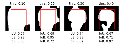
Figure 6: Examples of Jaccard-based metrics for several threshold values.

4 Implementation and Testing

Figure 7: VGG-19 network architecture with 1000 outputs corresponding to the 1000 classes used in training the network on a subset of the ImageNet dataset.

4.1 Implementation

We call our algorithm RSI-Grad-CAM (for “Riemann-Stieltjes Integrated Gradient Class Activation Map”. We implemented it using Keras over Tensorflow on Google Colab. We started with an implementation of Grad-CAM, and then modified it to replace the gradients with integrated gradients. A set of interpolated images between a (black) baseline and the final image are fed to the network, and activations and the gradients at the chosen layer are collected. For efficiency, the images are not fed to the network one by one, but in batches, in a similar way to what is done during network training. In theory the whole set of images could be fed as a single batch, but this tended to exhaust GPU resources, so we used limited size batches (32 images per batch).

The computation of the weights $w_{k}^{c}$ and the final linear combination of feature maps $\sum_{k}w_{k}^{c}A^{k}$ are straightforward. The application of a ReLU at the end allows to select only the units that contribute positively to the score of the selected class.

In our implementation, when computing the weights, we also selected only units in which activations, integrated gradients, and activation total increments $(A_{ij}^{k}(m)-A_{ij}^{k}(0))$ are all positive. This (inspired on the “guided Grad-CAM” approach of [Selvaraju 2017]) allows the algorithm to ignore extraneous elements that do not contribute to the chosen class score, e.g. if an image contains a ‘dog’ and a ‘cat’, and we are interested in locating only the dog, the area of the image containing the cat is expected to produce:

• negative integrated gradients for the network output corresponding to ‘dog’, and

• negative activations and activation increments in the feature maps more strongly linked to the ‘dog’ output.

As a consequence we expect that ignoring those units will produce sharper heatmaps better focused in locating the elements of the image related to the output of the chosen class. For the comparison to be fair we also used the Grad-CAM version with positive gradients in which weights are computed using equation (2).

After a heatmap has been produced at the layer level, it is upsampled to the original size and overlaid to highlight the elements of the input image that most contribute to the output corresponding to the desired class.

For the baseline we acknowledge that various choices are possible (black image, random pixels image, blurred image, etc.). In the present work we follow the choice suggested by the authors of the Integrated Gradients algorithm in [Sundararajan 2017] for object recognition networks, i.e., a black image.

4.2 Preliminary Testing

We compare our RSI-Grad-CAM to Grad-CAM and Integrated Grad-CAM on a VGG-19 network [Simonyan 2015].

The VGG-19 model consists of five blocks, each containing a few convolution layers followed by a max-pooling layer. For convolution operation, VGG-19 uses kernels of size $3\times 3$. The layers on each of its five blocks have 64, 128, 256, 512 and 512 channels respectively, as shown in Figure 7. The final layer has one thousand units and a softmax activation function, so its final outputs can be interpreted as a vector of one thousand probabilities, one per class.

Figure 8: First row: original image with 100% prediction probability; second row: heatmaps produced by Grad-CAM, RSI-Grad-CAM, and Integrated Grad-CAM respectively for the image; third row: overlaid heatmaps.

Figure 9: Heatmaps produced for a soccer ball on a paying field at the last block (left), and second to last (right).

Figure 10: Images with a German Shepherd and a cat. Heatmaps for the German Shepherd (top) and the cat (bottom). The score assigned to the cat is very low (0.22%), hence far from saturation, and in this case we do not expect Grad-CAM and RSI-Grad-CAM to yield very different heatmaps. The difference is more noticeable for the dog. Integrated Grad-CAM does a good job on this layer, separating correctly dog and cat.

Figure 11: Images of a set of guitar picks produced at the last convolutional block (left) and the next to the last block (right). Note how our RSI-Grad-CAM at the last block highlights the general area occupied by the set of picks, and it focuses on individual picks at the next to the last block. Grad-CAM produces dark heatmaps, and Integrated Grad-CAM fails to produce a useful heatmap at the last layer of block 4 (block4_pool).

All three attribution methods tested here are applied to the final pooling layer of each convolutional block. When we say that an attribution method is applied to the $n$th layer of the network that means “to the final polling layer of the $n$th block.”

Figure 8–11 show examples of scenarios in which our proposed approach RSI-GradCAM produces better visualization maps than Grad-CAM and Integrated Grad-CAM.

Figure 8 shows the heatmaps of an image for which the probability of the prediction by the network is 100%, so the output clearly becomes saturated. As expected, the output of the usual Grad-CAM is tenuous, while RSI-Grad-CAM yields a more visible heatmap. Integrated Grad-CAM produces a blurry heatmap a this level.

Figure 9 shows the heatmaps for a soccer ball at the last two layers. The network output for this image was 85.6%, far from saturation. Compared to Grad-CAM, at the last and second to last blocks of the network, Integrated Grad-CAM and RSI-Grad-CAM produce sharper heatmaps, better focused on the soccer ball.

Figure 10 illustrate the ability to locate two different elements in the same image. The network detects the German Shepherd and assigns it a 67.79% score, and the cat with 0.6% score. For the German Shepherd the heatmap produced by RSI-Grad-CAM is brighter and sharper than the one produced by Grad-CAM. The difference is less noticeable for the cat, for which the network output is far from saturation. The fact that the heatmaps highlight mainly the animal’s head is an indication that its body plays a lesser role in identifying the species. Integrated Grad-CAM does a good job locating both animals.

In general we observe that, when the network outputs are far from saturation, the heatmaps produced by our algorithm are similar to that of the the original Grad-CAM, the difference is more noticeable when the outputs are almost saturated. We also observe that the heatmaps produced by our algorithm look sharper and better focused in the area of the image that contains the desired element or feature.

Figure 11 shows heatmaps for a set of guitar picks. The probability predicted by the network was 100%, and the saturation of the output was so high that the heatmap produced by Grad-CAM was too tenuous to be visible. Heatmaps produced by our RSI-Grad-CAM highlights the whole set of picks at the last convolutional block (block5_pool layer), and individual picks at the next to last block (block4_pool layer). This example illustrates the fact that heatmaps produced at different layers highlight different aspects of the image: global (such as the general area occupied by the object of interest) when close to the output, and local details (such as individual parts) when produced at intermediate layers.

4.3 Quantitative Evaluations

The examples shown in the previous section are illustrative. Here we use the quantitative metrics introduced in section 3.4 to evaluate our attribution technique. For that purpose, we use a common image classification network working on a fairly large dataset with a variety of images of objects and natural elements, as detailed below.

4.3.1 Dataset and Model

We used the VGG-19 network pretrained on ImageNet [Simonyan 2015], with input shape $224\times 224\times 3$, and performed experiments on a subset of the validation dataset used for the ImageNet Large Scale Visual Recognition Challenge 2012 (ILSVRC2012) [Russakovsky 2015]. The ILSVRC2012 dataset is a subset of ImageNet with 50,000 images from 1,000 categories, annotated with labels and rectangular bounding boxes obtained using the Amazon Mechanical Turk [Sorokin 2008]. Figure 12 shows two randomly selected images with their bounding boxes.

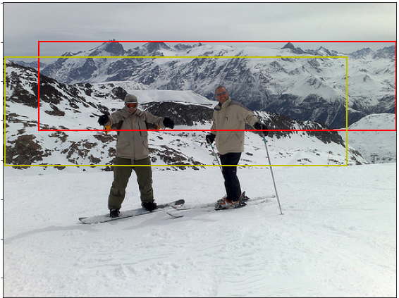
Figure 12: Two images from the ILSVRC2012 dataset. Left: image of Alp mountains with two bounding boxes. Right: image of a sea snake, with one bounding box. The bounding boxes are shown for illustration purposes only, the network was fed with images that didn’t display bounding boxes.

In all the tests we picked a convolutional block and computed heatmaps generated by each of the attribution methods at the maxpooling layer of the block.

The subset of images was chosen so that:

1. The network predicted the right class, to make sure that we are evaluating the attribution technique rather than the network performance.

2. The image contained only one bounding box, to avoid images with more than one category, or multiples occurrences of the same category.

3. The bounding box occupied less that 50% of the image area, because an object that occupies most of the image would be too easy to locate and would produce unreliably metrics.

The final dataset used contained a total of 12,525 images.

In the next section we compare the performance of Grad-CAM, RSI-Grad-CAM and Integrated Grad-CAM in three aspects: numerical stability, quantitative evaluations without ground truth, and quantitative evaluations with ground truth.

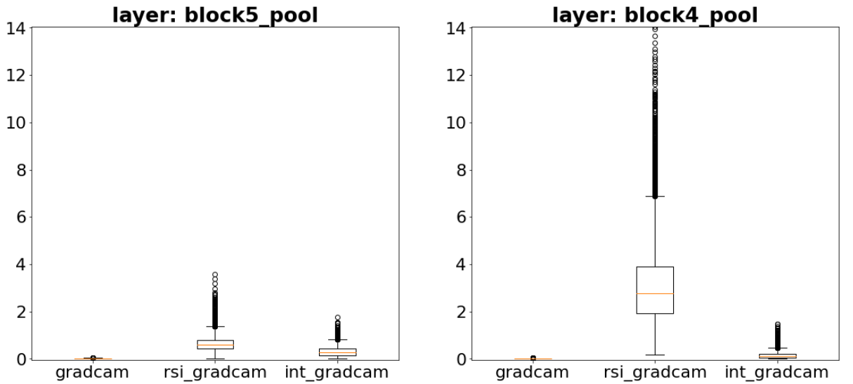
Figure 13: Boxplot of mean pixel values of heatmaps before normalization at the last two convolutional blocks.

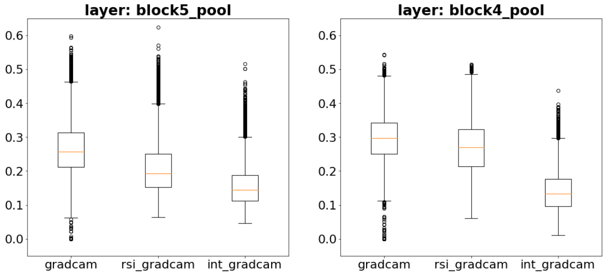
Figure 14: Boxplot of mean pixel values of heatmap after normalization at the last two convolutional blocks.

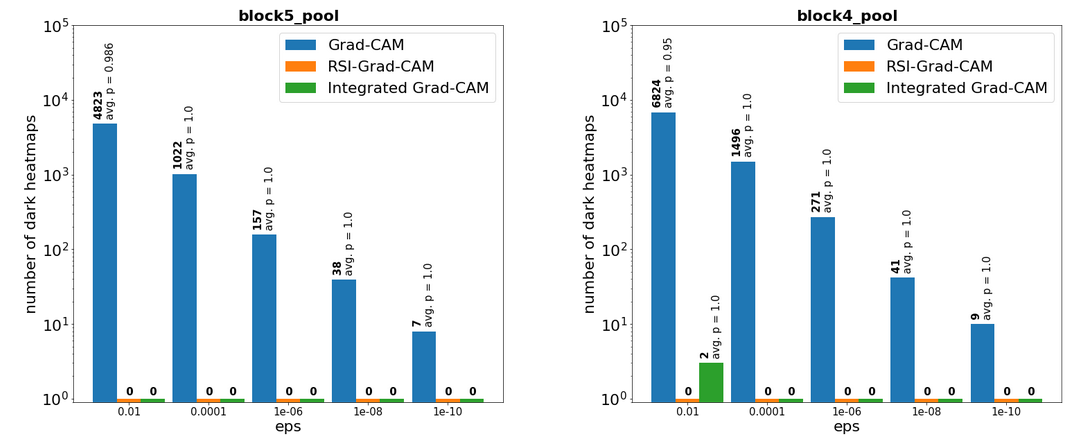
Figure 15: Number of dark heatmaps produced for the attribution methods applied to the last and next to the last blocks.

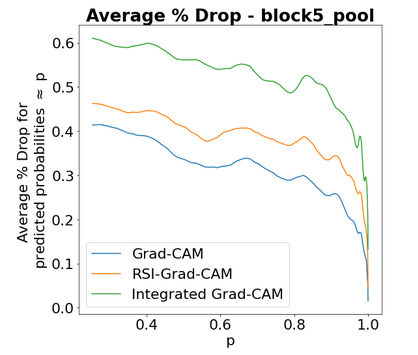
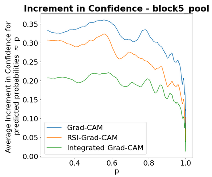
Figure 16: Average % Drop and Increment in Confidence at the last convolutional block.

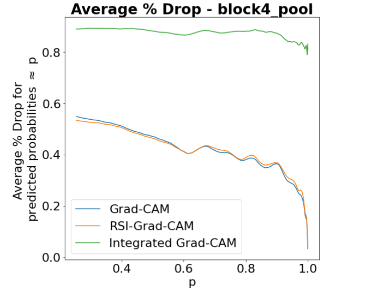
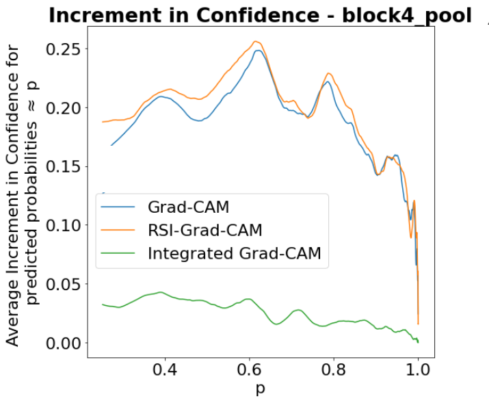
Figure 17: Average % Drop and Increment in Confidence at the next to the last convolutional block.

Figure 18: Energy at the last two convolutional blocks for each attribution technique. The colormap used to display the heatmap has been changed in this image to make the overlapping between heatmap and bounding box more visible.

Figure 19: Average energy at the last and next to the last convolutional blocks

4.3.2 Numerical Stability

As explained in section 3.4.1, low pixel values of heatmaps may introduce problems because of numerical instability. Figure 13 shows that Grad-CAM is particularly sensitive to this phenomenon. For each image we produce the corresponding (non-normalized) heatmap, and compute the mean value of its pixel values. The boxplots in Figure 13 show the distribution of mean pixel values of heatmaps produced for our database and model at the pooling layers of the last two convolutional blocks (block4_pool and block5_pool respectively) for each of the attribution methods tested.

We can see that the pixel values of the heatmap produced by Grad-CAM are very close to zero. This can cause the denominator of the fraction used for normalization of the heatmap to become zero or near zero, producing floating point underflow and unreliable results. In order to avoid division by zero or near zero we include a small term $\varepsilon$ in the bottom of the fraction used for normalization of a heatmap $L$, as shown in equation (26). In our tests we used $\varepsilon=10^{-8}$. Figure 14 shows the result of normalizing using this correction term.

We note that even after normalizing Grad-CAM is still producing some heatmaps with a mean value near zero. To avoid a blank heatmap, it is possible to reduce the value of $\varepsilon$ even more, although it is hard to tell exactly by how much without some trial and error.

We will define a dark heatmap as one in which its maximum pixel intensity is less than half the maximum possible range of pixel values, e.g. less than $0.5$ in a scale from 0 to 1: $(L_{max}-L_{min})/(L_{max}-L_{min}+\varepsilon)<0.5$. This happens precisely for $L_{max}-L_{min}<\varepsilon$ in equation (26). Note that the $0.5$ threshold value used in the definition of “dark heatmap” could be changed to some other value inside the interval $(0,1)$ without essentially changing the discussion below. E.g., if we replace it with $0.25$, the new “dark” images would look even darker, and there will be fewer of them, but that would not change the argument presented below in a meaningful way, it would just change the $L_{max}-L_{min}<\varepsilon$ condition to the one obtained from $(L_{max}-L_{min})/(L_{max}-L_{min}+\varepsilon)<0.25$, i.e. $L_{max}-L_{min}<\varepsilon/3$, so the analysis presented below would be the same just replacing $\varepsilon$ with $\varepsilon/3$. Other than that the barplots in Figure 15 would look the same, just with different numerical labels in the ’eps’ axis, and the comparison among the different attribution methods regarding the risk of producing “dark heatmaps” would be the same too.

Now we can count the number of dark heatmaps across the image dataset produced by a given attribution method applied to a given layer. The barplots in Figure 15 show the result of using various values of $\varepsilon$ (called ‘eps’ in the figure). Note that the plots are drawn using logarithmic scales. Here ‘avg p’ is the average value of the network output (probability of the input image belonging to the corresponding class) for all the images for which the attribution method produces a dark heatmap. It is included to show how it correlates with the number of dark heatmaps. We see that, for Grad-CAM dark heatmaps are produced when the network output gets close to $1$, the point at which it gets saturated and the vanishing gradient problem arise.

Another approach is to use Grad-CAM on the network with the final softmax layer removed to avoid the effects of vanishing gradients caused by saturation of the network output. In any case this shows the fragility of Grad-CAM, which may require to tweak parameters and network architecture to make it work. Integrated Grad-CAM and our technique RSI-Grad-CAM are not affected by these problems.

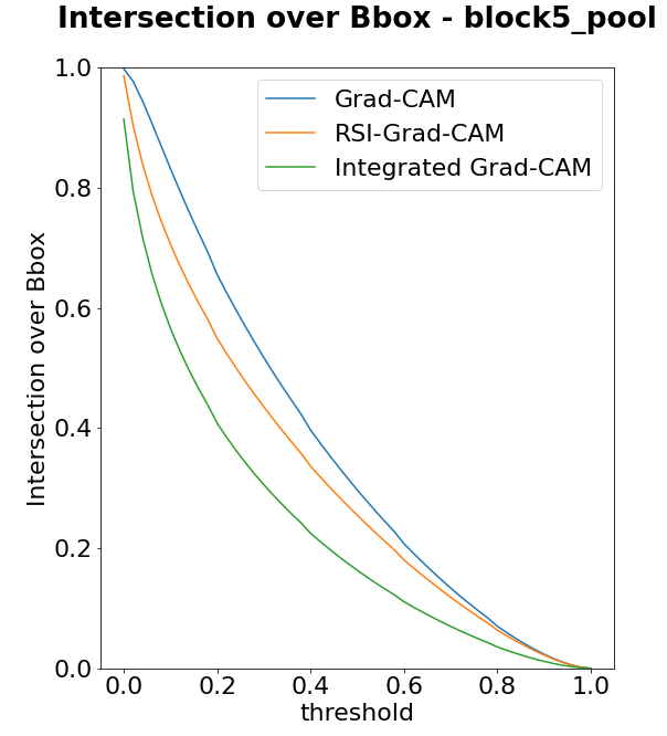
Figure 20: Intersection over Union, Intersection over Box, and Intersection over Region at the last convolutional block.

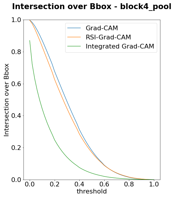
Figure 21: Intersection over Union, Intersection over Box, and Intersection over Region at the next to the last convolutional block.

4.3.3 Quantitative Evaluations Without Ground Truth (Results).

Now we look at the results of applying Average Drop and Increment in Confidence, introduced in section 3.4.2.

In order to determine if these metrics depend on the predicted probability, the graphics shown in Figure 16 and 17 were obtained by sorting the images by predicted probability, and computing averages across a fix length rolling window. In our experiments the window had a width of 1000 samples, so each point in the graph represents the average metric obtained for 1000 consecutive samples (the $p$ coordinate in the graph is also the average probability of the 1000 elements contained in the sliding window). We found that the performance of Grad-CAM was the best at the last convolutional block, but our method RSI-Grad-CAM did slightly better than Grad-CAM, while the performance of Integrated Grad-CAM got worse when computed at blocks below the last one.

4.3.4 Quantitative Evaluations With Ground Truth (Results).

Here we look at the results of applying Pixel Energy and Jaccard-based measures, introduced in section 3.4.3. Figure 18 provides an example of how the pixel intensity is distributed in relation to the bounding box. The results for the whole dataset (as a function of the probability $p$ predicted by the network) are shown in Figure 19. We observe that our method RSI-Grad-CAM performs better than Grad-CAM at the last and next to the last convolutional blocks of the network. Compared to Integrated Grad-Cam, RSI-Grad-CAM produces similar results at the last convolutional block, but again it performs better at the next to the last block.

On the other hand, the Jaccard-based measures depend on the threshold chosen, as illustrated in Figure 6.

Figure 20 and 21 show that, compared to the other methods, our RSI-Grad-CAM performs better for Intersection over Union at the next to the last block, indicating that a larger proportion of the heatmap tends to lie inside the ground-truth bounding box at that level. This is consistent with the effect shown in Figure 11, where the heatmap produced by RSI-Grad-CAM highlights internal structures of the object of interest (in this case individual picks in a set of picks). This makes our attribution method ideal in picking up middle level features of an image.

5 Conclusions

We have examined three attribution techniques intended to provide explanations about how CNNs make their predictions, and proposed a new method that better implements the goals of those techniques.

Grad-CAM uses gradients of the network output for a given class computed at an arbitrary convolutional layer. Those gradients are used to determine the relative contribution of each feature map in that layer to produce a heatmap highlighting the regions of the network input that contribute to the network output. While this technique works relatively well in many situations, its performance suffers when any of the network layers, particularly its output layer, is near saturation level. Integrated Gradients overcomes the problem caused by the network output saturation by integrating the gradients of the network outputs with respect to the inputs of the network along a set of outputs obtained by interpolation from a baseline to the desired input. However, it may miss features captured at hidden layers of the network.

Integrated Grad-CAM offers a solution based on integrating saliency maps. We include it here for comparison to our method, RSI-Grad-CAM. Unlike Integrated Grad-CAM, our RSI-Grad-CAM method replaces the gradients used by Grad-CAM with gradients integrated using the activations of the units of the internal layer as integrators. Compared to Integrated Grad-CAM, our method have comparable performances only when used at the last layer of the network, but the performance of Integrated Grad-CAM degrades quickly when used at hidden layers below the last one, and then our method performs better at those layers.

Compared to Grad-CAM we observe that the results of applying our RSI-Grad-CAM method yields better results when applied to images in which the network outputs are near saturation, has better numerical stability, and it is better suited to detect small details within the region of interest when used at layers right below the last one.

6 Future Work

Any method based on line integrals depends on the integration path used. In our algorithm we feed the network using a set of images linearly interpolated between a baseline and the desired input. A possible area of research would be to explore alternate integration paths.

On the other hand, there is a degree of arbitrariness in the choice of the baseline (a blank image in our case). Ideally the baseline should be an input that produces equal outputs for all classes. However it is unlikely that only one output has such property, so additional conditions on the baseline may need to be imposed depending on heuristic arguments (such as darker baselines being preferred to bright ones as indicative of “no features present”) and practical considerations such as final performance.

Another line of work would be to replace Grad-CAM with our RSI-Grad-CAM algorithm in existing works, such as the method proposed in [Chen 2020] for use in embedding networks.

References

- [Chattopadhyay 2018] A. Chattopadhyay, A. Sarkar, P. Howlader, and V. N. Balasubramanian (2018). Grad-cam++: Generalized gradient-based visual explanations for deep convolutional networks. In 2018 IEEE Winter Conference on Applications of Computer Vision (WACV), pages 839–847. IEEE, 2018.
- [Chen 2020] Lei Chen, Jianhui Chen, Hossein Hajimirsadeghi, Greg Mori (2020). Adapting Grad-CAM for Embedding Networks. arXiv preprint arXiv:2001.06538 [cs.CV]
- [Dhamdhere 2018] Kedar Dhamdhere, Mukund Sundararajan, Qiqi Yan (2018), How Important Is a Neuron? arXiv preprint arXiv:1805.12233 [cs.LG]
- [Hochreiter 1998] S. Hochreiter (1998), The Vanishing Gradient Problem During Learning Recurrent Neural Nets and Problem Solutions. Int. J. Uncertain. Fuzziness Knowl. Based Syst., vol. 6 (1998), pp.107–116.
- [Hochreiter 2020] Narine Hochreiter, Vivek Miglani, Miguel Martin, Edward Wang, Bilal Alsallakh, Jonathan Reynolds, Alexander Melnikov, Natalia Kliushkina, Carlos Araya, Siqi Yan, Orion Reblitz-Richardson (2020). Captum: A unified and generic model interpretability library for PyTorch. arXiv preprint arXiv:2009.07896 [cs.LG]
- [Horn 2012] Horn, Roger A.; Johnson, Charles R. (2012). Matrix analysis. Cambridge University Press. Chapter 5
- [Protter 1991] Protter M.H., Morrey C.B. (1991). The Riemann-Stieltjes Integral and Functions of Bounded Variation. In: A First Course in Real Analysis. Undergraduate Texts in Mathematics. Springer, New York, NY. https://doi.org/10.1007/978-1-4419-8744-0_12 sec. 12.2
- [Ribeiro 2016] Marco Tulio Ribeiro, Sameer Singh, Carlos Guestrin (2016), “Why Should I Trust You?”: Explaining the Predictions of Any Classifier. Conference: Proceedings of the 2016 Conference of the North American Chapter of the Association for Computational Linguistics: Demonstrations. DOI: 10.18653/v1/N16-3020
- [Russakovsky 2015] Russakovsky, O., Deng, J., Su, H. et al (2015). ImageNet Large Scale Visual Recognition Challenge. International Journal of Computer Vision (IJCV) 115, 211–252 (2015). https://doi.org/10.1007/s11263-015-0816-y
- [Sattarzadeh 2021] Sam Sattarzadeh, Mahesh Sudhakar, Konstantinos N. Plataniotis, Jongseong Jang, Yeonjeong Jeong, Hyunwoo Kim (2021), Integrated Grad-CAM: Sensitivity-Aware Visual Explanation of Deep Convolutional Networks via Integrated Gradient-Based Scoring. 2021 IEEE International Conference on Acoustics, Speech, and Signal Processing (ICASSP 2021)
- [Selvaraju 2017] Ramprasaath R. Selvaraju, Michael Cogswell, Abhishek Das, Ramakrishna Vedantam, Devi Parikh, Dhruv Batra (2017). Grad-CAM: Visual Explanations from Deep Networks via Gradient-based Localization. Proceedings of the IEEE International Conference on Computer Vision, 2017, pp. 618–626.
- [Shrikumar 2018] Avanti Shrikumar, Jocelin Su, Anshul Kundaje. Computationally Efficient Measures of Internal Neuron Importance. arXiv preprint arXiv:1807.09946 [cs.LG]
- [Simonyan 2015] Simonyan K, Zisserman A (2015), Very Deep Convolutional Networks for Large-Scale Image Recognition. arXiv preprint arXiv:14091556 [cs.CV]
- [Sorokin 2008] A. Sorokin and D. Forsyth (2008). Utility data annotation with Amazon Mechanical Turk. IEEE Computer Society Conference on Computer Vision and Pattern Recognition Workshops, 2008, pp. 1-8, doi: 10.1109/CVPRW.2008.4562953
- [Sundararajan 2017] Mukund Sundararajan, Ankur Taly, and Qiqi Yan (2017). Axiomatic attribution for deep networks. In Proceedings of the 34th International Conference on Machine Learning - Volume 70, ICML’17, p. 3319–-3328. JMLR.org, 2017.
- [Wang 2020] Haofan Wang, Zifan Wang, Mengnan Du, Fan Yang, Zijian Zhang, Sirui Ding, Piotr Mardziel, Xia Hu (2020. Score-CAM: Score-Weighted Visual Explanations for Convolutional Neural Networks. In Proceedings of the IEEE/CVF conference on computer vision and pattern recognition workshops, p. 24–25, 2020.
- [Williamson 2004] Williamson, Richard and Trotter, Hale. (2004). Multivariable Mathematics, Fourth Edition. Pearson Education, Inc.
- [Zhou 2016] B. Zhou, A. Khosla, L. A., A. Oliva, and A. Torralba (2016). Learning Deep Features for Discriminative Localization. In 2016 IEEE Conference on Computer Vision and Pattern Recognition (CVPR).