The Bold-Thin-Bold Diagrammatic Monte Carlo Method for Open Quantum Systems
Zhenning Cai
Department of Mathematics, National University of Singapore,
Level 4, Block S17, 10 Lower Kent Ridge Road, Singapore 119076
matcz@nus.edu.sg, Geshuo Wang
Department of Mathematics, National University of Singapore,
Level 4, Block S17, 10 Lower Kent Ridge Road, Singapore 119076
geshuowang@u.nus.edu and Siyao Yang
Department of Mathematics, National University of Singapore,
Level 4, Block S17, 10 Lower Kent Ridge Road, Singapore 119076
matsiya@nus.edu.sg
Abstract.
We present two diagrammatic Monte Carlo methods for quantum systems coupled with harmonic baths, whose dynamics are described by integro-differential equations. The first approach can be considered as a reformulation of Dyson series, and the second one, called “bold-thin-bold diagrammatic Monte Carlo”, is based on resummation of the diagrams in the Dyson series to accelerate its convergence. The underlying mechanism of the governing equations associated with the two methods lies in the recurrence relation of the path integrals, which is the most costly part in the numerical methods. The proposed algorithms give an extension to the work [“Fast algorithms of bath calculations in simulations of quantum system-bath dynamics”, Computer Physics Communications, to appear], where the algorithms are designed based on reusing the previous calculations of bath influence functionals. Compared with the algorithms therein, our methods further include the reuse of system associated functionals and show better performance in terms of computational efficiency and memory cost. We demonstrate the two methods in the framework of spin-boson model, and numerical experiments are carried out to verify the validity of the methods.
Key words and phrases:
Dyson series; inchworm Monte Carlo; bold-thin-bold Monte Carlo; integro-differential equation; fast algorithms
Zhenning Cai and Siyao Yang’s work was supported by the Academic Research Fund of the Ministry of Education of Singapore under grant A-0004592-00-00.
1. Introduction
It is a great challenge to numerically simulate a quantum system
coupled to its environment
to a non-negligible extent.
Nevertheless,
open quantum systems are
playing increasingly important roles
in many fields including
but not limited to
quantum computation [33],
quantum optical systems [1, 6],
quantum sensing
[12, 37],
and chemical physics [19, 40].
In general,
the main difficulty comes from
the coupling of the system
and the bath, which leads to
a non-Markovian process.
The non-locality of the simulation
generally requires large memory cost.
By using an influence functional
to describe the effect of the bath
to the system [16],
the iterative quasi-adiabatic propagator path integral (i-QuAPI) [22, 23]
assumes finite memory length
to prevent the unrestrained growth of the memory cost.
While the bottleneck of the i-QuAPI method is its memory cost,
some methods based on similar ideas
have been developed to further reduce the memory cost
and improve the computational efficiency.
For instance,
the blip-summed decomposition
eliminates a majority of system paths with small contributions [25, 26];
the differential equation based path integral (DEBPI) studies the continuous form of the i-QuAPI
and formulates a system of differential equations [39]
so that classical numerical methods can be applied.
Recently, the small matrix decomposition of the path integral (SMatPI) is proposed as a stable and efficient algorithm that overcomes
the exponential scaling of the memory cost with respect to the memory length [27, 28, 29].
Another main idea to simulate the system-bath coupling
is to use the Nakajima-Zwanzig generalized quantum master equation (GQME) [31, 44, 38, 43], which is an integro-differential equation describing the non-Markovian process of the system density matrix.
For a weakly coupled system,
one may neglect the memory effect
and work only on the Markovian approximation, resulting in the Lindblad equation [13, 20].
Methods based on the non-Markovian GQME includes momentum jump-GQME [18], which utilizes the surface hopping method in the computation of the memory kernel.
The transfer tensor method (TTM) for open quantum systems [7, 2, 10] can also be considered as a discretization of GQME.
It deduces the memory kernel of a time-nonlocal quantum master equation and reconstructs the dynamical operators, which can extend simulations to very long times.
Except for the deterministic methods,
another natural idea is to apply stochastic methods for the high-dimensional integrals in the Dyson series [14].
The diagrammatic quantum Monte Carlo (dQMC) method uses diagrams to better visualize the coupling between the system and the bath [35, 41].
In this method, the memory cost is no longer an issue, but it suffers from the numerical sign problem [21, 4],
where the variance increases exponentially
with respect to the simulation time .
To tame the sign problem,
different techniques are developed.
The inchworm Monte Carlo method is one of the recent successful improvements, which applies “bold-line diagrams” to
accelerate the convergence of series [8, 9, 3, 42, 4]. It has achieved many successes in the computation of impurity models [11, 36, 15]. The idea of using bold lines can be traced back to [34], and has been applied to the impurity model in [17]. In general, a bold diagram is the sum of a number of original diagrams denoting the terms in the Dyson series. By clustering some diagrams in the Dyson series, the total number of diagrams to be summed is reduced, and hence improves the numerical efficiency.
In [5],
the authors design a fast algorithm
that reuses the samples generated in previous time steps to reduce the calculations of the bath influence functional without losing accuracy of dQMC and the inchworm Monte Carlo method.
In this paper,
we further discuss the reuse of previously calculated results based on the intrinsic invariance of the quantum propagators.
For the computation of Dyson series,
we explore a recurrence relation of the series to be computed at each time step, and
propose a fast algorithm
that requires a much smaller amount of new samples at each time step.
While this idea can not be directly applied to the inchworm Monte Carlo method, we modify the inchworm Monte Carlo method by allowing some thin lines in the diagrams, and develop
a new “bold-thin-bold” (BTB) Monte Carlo method
where the recurrence relation can again be formulated and the fast algorithm can also be designed. The name “bold-thin-bold” describes the typical structure of the diagrams, where a thin line is sandwiched between two bold sections.
For the rest sections of this paper,
we present the derivation of the fast algorithms for Dyson series and the BTB method.
In Section2,
we first introduce the spin-boson model
and the Dyson series,
and then design a fast algorithm
for the computation of Dyson series
based on a recurrence formula. Section3 contributes to the derivation of our new diagrammatic Monte Carlo method.
In Section3.1,
we give a brief introduction to inchworm Monte Carlo method
and its diagrammatic representation.
In Section3.2,
the BTB method is presented intuitively by diagrams
and formally by equations.
The fast algorithm
for BTB method is designed
based on the recurrence relation
in Section3.3.
At the end of both Section2 and Section3,
some remarks about the number of samples required
and the comparison between methods are given for better understanding. In Section4,
we carry out some numerical experiments
to illustrate the validity of our algorithms.
Some discussions about the computation efficiency
and the variances of two methods
are also given in Section4.
In Section5,
we briefly conclude the idea of the whole paper
and discuss the possible future work.
2. Fast algorithm for Dyson series
2.1. Spin-boson model and Dyson series
We study the density matrix of the system-bath dynamics in an open quantum system, which can be described by the following von Neumann equation:
(1)
The Hamiltonian is an operator on the Hilbert space , where and
represent the spaces associated with the system and bath, respectively. The Hamiltonian can be written as the sum of three parts, the system, the bath and their coupling:
where are operators on and are operators on . The identity operators
are defined over the system space and bath space , respectively.
The coupling term is assumed to have the tensor-product form
In such an open quantum system,
we are generally indifferent to the evolution of the bath.
However, as the system is coupled with its bath,
the effect of the bath cannot be neglected, which introduces significant difficulties in the simulation of open quantum systems.
In this paper, we only consider spin-boson model,
where the system is a single spin
and the bath is modeled by a large number of harmonic oscillators. While the algorithms proposed in this work can be easily generalized to any multiple-state open quantum systems, the spin-boson model contains most difficulties for the simulations of system bath dynamics and thus is used as a fundamental example throughout this paper to demonstrate our methods.
2.1.1. Spin-boson model
In the spin-boson model, the Hilbert spaces are
with being the space over
and is the index of harmonic oscillators in the bath.
Additionally, the Hamiltonians and coupling operators are given by
The notations used in the equations above are defined as follows:
•
Pauli matrices: , .
•
: The energy difference between two spin states.
•
: The frequency of the spin flipping.
•
: The momentum operator of the th harmonic oscillator, .
•
: The position operator of the th harmonic oscillator, .
•
: The frequency of the th harmonic oscillator.
•
: The coupling intensity between the spin and the th harmonic oscillator.
The solution to (1) can be formally written as .
With the assumption that the system and bath are not entangled initially ,
the expectation of a given observable over the system can be computed by
We define the propagator
where is the partial trace operator with respect to bath.
With this propagator, with is the partial trace operator with respect the system.
One may check that this propagator is Hermitian, i.e, .
2.1.2. Dyson series
It is practically prohibitive to compute directly
because of the high dimensionality of the bath space .
In mathematical physics,
the time evolution operator in the interaction picture can be expanded as Dyson series [14, 3, 5]:
(2)
where the variable of integration is an -dimensional vector
and its integral domain is an -dimensional simplex
and thus the integral in (2) should be interpreted as
In the integrand, the notation denotes the number of negative components
in , and
describes the contribution of the system dynamics, which is defined by
(3)
where
(4)
The bath influence functional satisfies the following Wick’s theorem [32]
where is a complex-valued functional
(5)
with
and being the spectral density.
The set is given by
(6)
For example,
and the corresponding bath influence functionals are formulated as
Inserting the definition of into (2), the series now only sums over the even terms as the bath influence functional vanishes when is odd:
(7)
The above expansion of Dyson series can also be expressed by the following diagrammatic representation:
(8)
where the propagator on left-hand side is denoted by a bold line. On the right-hand side, each diagram represents an integral of the form
In detail, each thin line segment connecting two adjacent time points
and means a bare propagator
appearing in the system associated functional ;
a black dot at introduces a perturbation operator in ;
an arc connecting and stands for the two-point correlation .
In particular, the first term on the right-hand side of (2) is denoted by a thin line with no dots or arcs (the first diagram on the right-hand side of (8)).
In general, the integral over time points
(9)
which appears in the expansion of (see (7)), is the sum of all possible combinations of the pairings of , which includes diagrams in total. For example, when , the integral (9) is diagrammatically represented by
To evaluate using the series expansion (7), one natural idea is to truncate this Dyson series at for a sufficiently large even integer and compute the high-dimensional integrals using Monte Carlo method, resulting in the method of bare dQMC [35, 41] which evaluates by
(10)
where for simplicity, the Monte Carlo samples are drawn independently according to the uniform distribution with , and in the formula above is the volume of the domain of integration . One may also apply other sampling strategy in general.
Alternatively, we can also solve via the following integro-differential equation, which is obtained by taking time derivative on both sides of (2) (see [5] for the derivation):
(11)
where stands for the series:
(12)
and the initial condition is given by according to definition (2). Here we use the notation to denote the series with expression (12) in order to distinguish it from other formulations of to be introduced later in this paper.
Note that now in the function , the last time point is fixed as , and thus the series on the right-hand side now sums over odd . Diagrammatically, this series is written as
(13)
With this integro-differential equation, one can solve iteratively by Runge-Kutta method. Throughout this paper, we apply the second-order Heun’s method, which reads
(14)
where is the time step length. The initial condition is given by . is the approximated solution of with , and approximates again by truncating the series and replacing the integrals by the average of Monte Carlo samples:
(15)
In th time step, the samples are drawn from uniform distribution . In practice, the number of samples is assumed to be proportional to the integral of the absolute value of bath influence functional
The two-point correlation is then replaced by some empirical constant , which yields
(16)
where is some positive constant. In practice, we may first assign the value of , then the general is set to be the nearest integer of the value (16).
Compared with the bare dQMC (10), the numerical methods based on (11) preserve the Hermitian property of as the right-hand side of (11) is always Hermitian, while this is not guaranteed by bare dQMC which directly evaluates the Dyson series (2).
With the time evolution of provided by the numerical scheme, we are ready to propose our fast algorithms based on calculation reuse which will be detailed in the following section.
2.2. Numerical method based on reuse of calculations
The main idea of the reuse of calculations concentrates on the following relations of the bare propagator and two-point correlation :
Proposition 1.
Given any and , we have
•
The bare propagator (4) associated with the system satisfies
The rigorous proof for the relations above can be found in the appendix of [5]. These relations describe the invariance of and after “shifting” or “stretching” by the time step length . We hope to utilize such properties to reuse the previous calculations in the scheme (14). In fact, one can easily use (18) to derive the following property.
Proposition 2.
Given and such that and , define
(19)
we have
(20)
In [5], fast algorithms that avoid duplicate computations of have been proposed based on such invariance of the bath influence functional.
Specifically, suppose we have sampled time sequences and calculated the corresponding bath influence functionals for (15). Then at the next time step, we can use as part of the samples to compute so that can be directly obtained by (20). One may refer to [5] for more details.
However, due to the existence of the observable in the definition of (4) when , there is no similar invariance for the system associated functional . Consequently, in the reuse algorithm developed in [5], needs to be evaluated with all samples at each time step. In the rest of this section, we propose a new fast algorithm for Dyson series which can achieve the reuse of as a whole. To do this, we introduce the linear basis of , and :
Definition 3.
Given two states and , we
define
(21)
(22)
and
(23)
With the definitions above, the bare propagator for can now be expressed as the linear combination
(24)
where the coefficients satisfies that
(25)
Inserting (24) into (3), the system associated functional is written as
linear combination of :
and thus we may express
At this point, we can rewrite the original integro-differential equation (11) as
(26)
which can again be numerically solved using a discretization similar to (14). Under such scheme, we aim to find some recurrence relation of the basis so that it can be computed iteratively.
Below we begin with the iterative relation of :
Lemma 4.
Given two states and , we have
(27)
where the coefficients satisfy that
(28)
Proof.
For the bare propergator with ,
directly using the definition (21) yields that
(29)
Insert the formula above into (22), due to (17),
we arrive at
Note that the coefficients depend only on the observable, the Hamiltonian and the time step .
Therefore, coefficients can be computed offline for any given time step . At the time step , we now split the -dimensional integral in as
(30)
where the domains of integration on the right-hand side are defined as follows:
Definition 5.
Given , and ,
and
The sum of the first integral on the right-hand side of (30) over all odd can be directly obtained using the previous calculations of :
where we have used (20) and (27) in the derivation. The second integral on the right-hand side of (30) has to be evaluated at each time step. This implies the following recurrence relation of summarized in the following theorem:
Theorem 6.
Given and ,
we have
(31)
where is defined by
The recurrence relation above will be used in each time step of the Heun’s scheme for (26) to achieve reuse of calculations. Similar as (15), the series to be newly computed is truncated by some odd integer and the integrals are evaluated using Monte Carlo method. The details of such a procedure are described in Algorithm 1. In the input, denotes the number of total time steps, and the number of samples is similarly given as (16) with the volume of simplex replaced by the volume of :
(32)
Algorithm 1
1:input , , ,
2:Set , (zero matrix), , for and
3:Compute according to (25), according to (28) for
To end this section, let us have a brief discussion on the computational and memory cost of Algorithm 1. In particular, we compare it with the direct implementation of Heun’s scheme (14) without using the recurrence relation, as well as the existing reuse algorithm in [5] which avoids duplicate calculations of the bath influence functionals.
Below we list the total computational cost on the Monte Carlo integration in the three approaches:
Here and are respectively the computational cost of the system associated functional and the bath influence functional with a given point time sequence. Asymptotically, is evaluated with the computational cost at by the definition (3), and can be computed with the cost at upon applying the inclusion-exclusion principle [42]. For large , in the three approaches is negligible, so that (34) and (35) will have similar values, which reduce the original cost (33) by a factor (see the complexity analysis in [5, Section 2.5]). However, when is small, is comparable to , and then the ratio of (35) to (34) will be at asymptotically using the formulas of and . In this sense, the algorithm in the current work can considerably improve the computational efficiency particularly in the weak system-bath coupling regime.
Moreover, Algorithm 1 requires a lower memory cost compared to the algorithm in [5]. In 7 and 8 of Algorithm 1, where the major computations concentrate in, one may draw a single sample each time and compute the corresponding , which is added to the summation in 8 and can then be discarded. In this process, the memory cost can stay low since we only need to store and for , which are essentially eight two-by-two matrices in total. The algorithm in [5], however, requires in total such matrices to store the infinite series for all time steps. We refer readers to [5, Section 2.4] for the details.
3. Bold-thin-bold diagrammatic Monte Carlo method
It is well known that the methods based on direct summation of the Dyson series usually suffer from the numerical sign problem [21, 30, 41] for long-time simulations.
To tame the sign problem, bold lines, which are usually the sum of many diagrams, have been introduced in a number of methods to reduce the number of diagrams [17, 11].
Among these methods, the inchworm Monte Carlo method has been successfully applied to models including quantum impurity problems and exact non-adiabatic dynamics [8, 9, 3, 4].
Below, we will first review the inchworm Monte Carlo method in the context of spin-boson model.
Our review will be based on the reformulation of , which is a perspective slightly different from the literature [8, 3].
We will then modify this approach to derive a novel diagrammatic Monte Carlo method that also has the iterative structure introduced in Section2.2.
3.1. Review of inchworm Monte Carlo method
In open quantum systems, the bold lines are defined to be the partial resummation of the Dyson series. In [8], the bold lines are introduced as “full propagators” , defined as
(36)
where is given in (4) and the system associated functional is formulated as (3) with replaced by and . The following properties of the full propagator will be found useful later in this paper (see their proofs in [5]):
Proposition 7.
•
Shift invariance: For any , if or , we have
(37)
•
Conjugate symmetry: For any , we have
(38)
•
Jump condition: is discontinuous on the line segments
and . At the origin, we have
(39)
(40)
We remark that the initial condition of the integro-differential equation (11) is a result of jump condition (40) as . Later we will see that other solvers for the full propagator may use (39) as the initial conditions.
The central idea of inchworm method [3] lies in the resummation of the series in the governing equation (11) using the previous calculations of the full propagators.
Diagrammatically, the full propagator is represented by a bold line segment connecting the initial time point with the final time point . This is consistent with (2) when and . The inchworm method then replaces all the thin line segments in the diagrams (13) by bold line segments, and then removes some diagrams from the summation to maintain the equality. For example, the first diagram on the right-hand side of (13) is replaced by
(41)
By (36), the two bold line segments above can be expressed as
(42)
Inserting the above formulas into (41) yields that
(43)
which includes all the thin diagrams where the arc connecting to does not intersect with any other arcs. These diagrams form a subset of the diagrams in (13), and thus (41) can be considered as a partial sum of . For example, the first, second and fourth diagram in (13) are included in (43) while the third diagram is not since the two arcs have an intersection.
Therefore, on the right-hand side of (13), after replacing the thin line segments in the first diagram with bold line segments, the second and the fourth diagrams, as well as infinite other diagrams in (43), should be removed.
Then, for the third diagram, we again replace all the thin line segments with bold line segments:
which can also be expanded into infinitely many diagrams, and we will remove these diagrams from (13) to maintain the equality.
We can continue such a process of replacements and removals, and eventually the series will be expressed as the sum of bold diagrams only:
(44)
In these diagrams, all the arcs are “linked”, meaning that any two time points can be connected with each other using the arcs as “bridges”. We remark that such resummation includes all diagrams shown in (13) and no diagram is double-counted. One may refer to [3, Section 3.3] for the rigorous proof. Mathematically, we may use the subset to denote the collection of all linked pairings. The superscript here refers to “connected”. For example,
Note that here is odd, and thus has arguments. Similarly, the infinite series can be approximated by truncating to some large odd and evaluating the high-dimensional integrals via Monte Carlo method. Such a numerical solver is known as the inchworm Monte Carlo method. Compared with the Dyson series defined in (12), working with is advantageous as the its convergence with respect to is faster since each diagram in (44) includes infinite diagrams in (13). In addition, given any , the inchworm Monte Carlo method only considers linked pairings and thus contains fewer diagrams than (13), making the direct evaluation of the bath influence functional cheaper than in the Dyson series.
In order for efficient implementations, we examine the possibility of applying the idea of iterative calculations proposed in Section 2 to the inchworm Monte Carlo method, which requires several invariant properties for the functionals in the reformulated . It is not hard to observe that the bath influence functional satisfies the invariance similar to (20):
according to (18), and the shift invariance (37) produces the similar result as (17). However, when , it is not clear whether we can write as a linear combination of some simple basis as in (21). As a result, a decomposition similar to (29), which plays a key role in our iterative algorithm, is unavailable for . This indicates that special treatment for the propagators is needed when crossing the time 0 to make our fast algorithm applicable.
3.2. The bold-thin-bold diagrammatic Monte Carlo method
In this subsection,
we will modify the current inchworm Monte Carlo method
by considering another resummation of
such that the idea of our iterative scheme for Dyson series can again be applied.
Instead of replacing all bare propagators in Dyson series by full propagators, we replace them by
(46)
Such expression allows us to define its linear basis analogous to (21):
(47)
which immediately gives us the similar result as (29):
(48)
With the above desired invariance satisfied, one can now repeat the analysis for Dyson series to obtain a formula similar to Theorem 6, based on which the reuse algorithm can again be applied. We postpone the details in Section 3.3. For now, let us focus on how the series will be reformulated upon replacing all by . In particular, we are interested in the new bath influence functional after this replacement.
In the diagrammatic representation, all the thin line segments are replaced by the corresponding bold line segments only when they do not include time 0. Below, we will derive the integro-differential equation based on these propagators following the “replace and remove” procedure introduced in the previous subsection. Again, we start from the first diagram in defined by (13). But now we split this diagram into two subdiagrams:
(49)
Here the time 0 is marked explicitly in the diagrams, and the location of with respect to time 0 indicates the domain of integration. When upgrading thin lines to bold lines, we will not change the line segments containing the zero point. This can be automatically achieved by replacing with :
(50)
Similar to (43), one may expand the bold line segments as Dyson series by inserting the expressions (42) to find the thin diagrams included in (50). Clearly, the two diagrams in (49) are included. In addition, the following diagrams with two arcs
as well as infinitely many other diagrams with more arcs also appear in (50). These diagrams should be removed from the sum after replacing (49) with (50), and these newly introduced diagrams in (50) which combine thin and bold line segments can again be considered as partial sums of . To proceed, we split the diagrams with two arcs in (13) by adding the zero point:
(51)
As mentioned previously, the two diagrams in the boxes are already included in (50), and do not need to be considered any more. For other diagrams on the right-hand sides, we again replace them with the new diagrams by changing to , and delete the thin diagrams included in these diagrams. By repeating this process, the resummation can be written as
(52)
Here we only draw diagrams with up to three time points for conciseness. The formula above shows that most diagrams have a thin line including zero sandwiched by two bold lines. We therefore call the stochastic method based on (52) the “bold-thin-bold diagrammatic Monte Carlo” method, or the BTB method in short.
Mathematically, we use the notation to denote the set of pairings with nodes that are preserved in (52). Similar to for the inchworm method, is again a subset of . However, since the location of time 0 is taken into consideration now in each diagram, the definition of relies on the distribution of . For example,
In general, the set is given by the following definition:
Definition 8.
Given and for some even ( if ), the set is defined by its complement in :
for ,
we have iff there exists a subset
satisfying the following two properties:
(a)
is a set of consecutive integers in ;
(b)
or where and .
The set includes all possible pairings in the Dyson series (13) that have been removed when we replace thin lines with bold lines. Therefore, the pairings in is then given by .
To better understand the reason for such a definition, we provide in Figure1 two examples of pairings in . Note that for all the pairings in , the last time point always equals . In Figure1a, the diagram represents the set with , and its subset (the red arc) satisfies both conditions in Definition8. The reason why this diagram should be excluded from the summation (52) is that all the thin diagrams it includes have already been counted in the second diagram in (52). Similarly, for Figure1b, which is the diagrammatic presentation of with , we can choose and find that . In fact, this diagram is a partial sum of the eighth diagram in (52), and thus should be excluded. Generally, the condition (b) requires that the subset does not include any end points of the “bold sections”, which refers to the interval for Figure1a and the intervals and for Figure1b. In this case, the diagram represented by , which has fewer points, embraces completely, and therefore all the diagrams in should not be considered in (52).
(a)
(b)
Figure 1. Examples of diagram with pairings .
As a comparison, the diagrams given in Figure 2 are pairings in , which should be counted into the series (52). Although these diagrams also have proper subsets with consecutive integer indices (red arcs in Figure2), the subdiagrams all touch the ends of the bold section, and thus cannot be removed to generate fewer-point diagrams that include them. For example, the first diagram in Figure2 can be written as with . If we remove the points and from , the resulting diagram is the first diagram in (52), which does not include . Other diagrams in Figure2 should be preserved due to the same reason.
Figure 2. Examples of diagrams with pairing .
At this point, we can express the resummation mathematically by
(53)
where
The evolution of is again solved numerically based on the governing equation (11) together with the resummation . This BTB method can be considered as an intermediate approach between Dyson series and inchworm method. Compared to the Dyson series, the BTB method has faster convergence with respect to as many thin line segments of the diagrams in are now replaced by bold ones which include infinite subdiagrams. However, as the propagator crossing time 0 remains to be a thin line segment for the purpose of reuse algorithm, the convergence of BTB method should be slower than that of inchworm method. This also implies that the number of diagrams considered in BTB method is smaller than Dyson series but larger than the inchworm method (see Table 1). Hence, if we directly evaluate the three bath influence functionals , and for the same by summing up the corresponding diagrams, the computation of is the fastest, and the computation of the slowest.
1
1
1
1
1
3
3
1
2
3
5
15
4
6
12
7
105
27
36
66
9
945
248
310
510
11
10395
2830
3396
5100
Table 1. Number of pairings in , and for . Note that the value of relies on the distribution of and thus we list both the smallest and largest value.
Although the BTB method has more diagrams than the inchworm method, the BTB method can save a significant amount of computational cost by using the recurrence relation (48). More importantly, later we will see the inchworm method needs to deal with two time variables, while the BTB method is essentially a one-dimensional problem. The details will be discussed in the following subsection.
3.3. Numerical scheme for the BTB method
We now elaborate the iterative algorithm for BTB method. With the linear basis (47), we can define
(54)
and
(55)
which are analogous to (22) and (23), respectively. Then resummation (53) is then formulated as
where is given as (25). The shift invariance (37) of
and the recurrence relation (48) of
yield
following the analysis for Lemma 4. In addition, it is also easy to check that
Eventually, we may arrive at a recurrence relation similar to (31) which plays a key role in the reuse algorithm computing as
(56)
where
(57)
and the coefficient satisfies (28), which depends on the time step . In order to compute numerically, we need the following approximations:
•
Truncation of the infinite series at ;
•
Application of the Monte Carlo method to compute the high-dimensional integrals;
•
A numerical scheme to calculate the system factor .
While the first two points are also implemented in
Section2.2, the third point requires some extra effort for the BTB method. Using the shift invariance (37) and the conjugate property (38) of the full propagator, we can rewrite the definition of as
(58)
where is defined by the limit
Thus, according to the definition (54), the computation of requires the knowledge of for . In our implementation, we will first compute for all . Let
(59)
Then for any , the value of can be approximated by piecewise linear interpolation. The interpolant can be written as
(60)
We can then let
and thus
(61)
is a practical approximation of .
At this point, we can again solve numerically by Heun’s scheme (14) following the procedures in Algorithm 1 where 7 and 8 are now replaced by the approximation of :
where
The evaluation of is based on the following generalized inchworm integro-differential equation [3]
(62)
where
The numerical solver of (62) can again be constructed by combining Huen’s method and the Monte Carlo intergration:
(63)
The initial condition of the scheme above is given as according to (59). The interpolating functional is defined similarly to (61):
and in the second stage is given by the same formula as with all replaced by the interpolated function satisfying
The samples are drawn from uniform distribution .
Similar to (16), the number of samples is again set to be proportional to the volume of the integration domain:
In our implementation, we choose to be the same as used in (16).
As a summary, our BTB method consists of two stages. The first stage solves the function from (62) using the scheme (63), and the second stage runs a procedure similar to Algorithm1, with suitable alterations to change bare diagrams to the BTB diagrams. Due to the larger number of samples in the second stage, we expect that the computational cost of the second stage is dominating. Compared with Algorithm1, the BTB method may also have lower computational cost for large due to the smaller number of diagrams. This will be verified by our numerical tests in the next section.
At the end of this section, we would like to compare the BTB method with the inchworm Monte Carlo method. Both methods use bold diagrams to mitigate the numerical sign problem. However, the BTB method only uses bold lines on one side of the zero, allowing us to use the shift invariance to reduce all the bold lines to a one-variable function (see (58)); the inchworm method uses with and , so that the full propagator must be computed as a two-dimensional function. Thus, compared with the inchworm method, the BTB method reduces the number of propagators to be computed by a factor of . Moreover, although the inchworm method also allows reusing computed influence functionals as proposed in [5], all the samples and the influence functionals must be stored, which may lead to a significant memory cost. The superiority of the inchworm method is its faster convergence with respect to . Based on these reasons, the BTB method is believed to be superior when the coupling is not too strong, while the inchworm method is preferable when the numerical sign problem is severe.
4. Numerical results
In the following experiments,
we choose the spectral density in (5) as
(64)
with being the Dirac delta function
and given by
(65)
where is the number of harmonic oscillators in the bath.
These parameters correspond to the bath with Ohmic spectral density [24].
With the spectral density ,
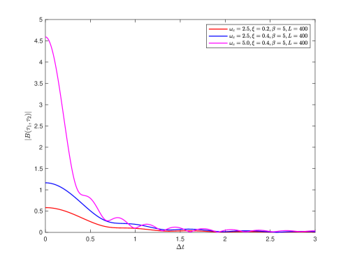
function (5) becomes
where .
From the above expression,
the amplitude of the function
depends on the parameters and .
We therefore plot the amplitude of the function
for the sets of parameters we use
in this paper in Figure3.
From Figure3,
the amplitude of
increases as either or increases.
Larger amplitude of function indicates stronger coupling between the system and the bath,
which in general brings difficulty to numerical simulations.
Figure 3. The amplitude of function for different parameters.
For all the experiments,
the number of harmonic oscillators is assumed to be ,
the maximum frequency is chosen as
and time step is chosen to be 0.05.
Other parameters will be specified for each experiment.
All the experiments in this paper are run on the CPU model “Intel® Core™ i5-8257U”, and four threads are used in the numerical simulations.
4.1. Experiments with different biases
We first check the validity of our method
by using the following parameters:
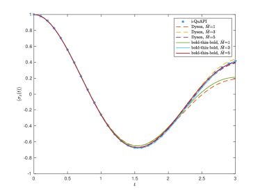
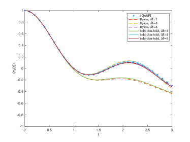
with two different biases and .
The results of both Dyson series and BTB method are shown in Figure4.
The i-QuAPI results are also plotted for reference.
(a)
(b)
Figure 4. Evolution of with and .
The number of samples is determined based on (32) with .
Figure4 shows that truncating
(12)(53) with
leads to significant numerical errors around in both cases, while remarkable improvement is made when is increased to , yielding curves well matching the ones generated by i-QuAPI and . The convergence towards the same curve in both methods validates our iterative algorithm for the spin-boson model with or without energy difference.
With these sets of parameters,
the two-point correlation defined in (5)
has a relatively small amplitude according to Figure3,
leading to a fast convergence with respect to for both series in (12) and (53).
In our implementation, the empirical constant in (32)
is chosen as a sixth of the largest amplitude of the function , which equals in these two examples.
Consequently, the number of samples required in the Monte Carlo sampling is relatively small, and the computational time for both methods is less than 20 seconds.
In our experiments, we find that the simulation based on the Dyson series is slightly faster than the BTB method. This is because BTB method needs extra computations on by (63) which is not required for Dyson series. A closer study on the computational time will be carried out in the next subsection.
4.2. Experiments for different frequencies
One critical problem of the Monte Carlo based methods
for open quantum systems is the sign problem.
The analysis in [3, Section 5] shows that the severity of the numerical sign problem is mainly characterized by the magnitude of the two-point correlation function .
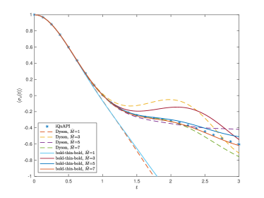
To test the performance of both methods in the case where has a larger amplitude, we choose the following parameters:
with frequencies and .
According to Figure3,
the increase of both and
will lead to a greater amplitude of , indicating
stronger coupling between the system and the bath.
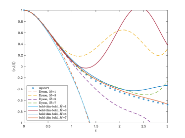
The results of both methods up to are given in Figure5.
(a)
(b)
Figure 5. Evolution of with and .
The number of samples is determined based on (32) with .
In these experiments, early truncations of the series at
are insufficient to approximate the series due to the stronger coupling.
In general, for a fixed ,
the BTB method provides more accurate results thanks to the use of bold lines.
For example, in Figure5a,
if we compare the results with legends “Dyson, ” and “BTB, ”,
it can be observed that the result of BTB method is valid for all ,
while the result of Dyson series starts to deviate from the reference solution provided by i-QuAPI at .
In addition to the accuracy,
another advantage of BTB method over Dyson series is
its better efficiency.
For the same value of , the computation time of BTB method is shorter since the number of diagrams in is
smaller than that in (see Table1).
When is large,
the computation time of BTB method is significantly shorter compared to Dyson series.
Table2 lists the wall clock time for the tests in Figure5.
From Table2,
it is clear that when , BTB method only takes about a third of the time
that the Dyson series takes.
Another reason leading to this difference is that
for each sample, Dyson series requires the complicated computation on the matrix exponential in each . For BTB method, most of these expensive are replaced by the cheaper bold lines which are obtained from linear interpolations. The difference in the wall clock time between the experiments with and
is due to different choice of the empirical constant .
For , the constant is set as 0.1942, while for the constant is 0.7652 ().
According to (32),
the number of samples for
is about times as that for when , which explains
the enormous difference between the two experiments.
Dyson
BTB
Dyson
BTB
1
3
17
8
56
3
24
34
312
290
5
73
58
3228
1698
7
241
115
53225
16086
Table 2. Comparison of wall clock time (round to nearest second) for tests in Figure5.
4.3. Variance test
The severeness of sign problem
can be measured by the variance of the results.
Therefore, we carried our an experiment
to numerically evaluate the variance of each method.
The parameters is the same as what we used in Section4.2:
In the test, we use the truncation dimension and as reference solutions,
which are denoted by for the method based on Dyson series and
for the BTB method.
We set and repeat the same experiments times.
The corresponding results are denoted by
and
for .
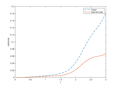
The variance of the methods are then numerically evaluated by
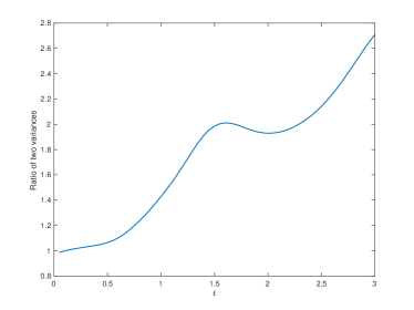
We then plot the result and in Figure6a and their ratio in Figure6b.
(a)
(b)
Figure 6. The change of variances , and the ratio with respect to (repeat times ).
As is shown in Figure6a,
the variance of the BTB method
is lower throughout the simulation.
At , the variance of both methods are and respectively.
This indicates
that the BTB method can better
tame the numerical sign problem.
We also observe in Figure6b that as time evolves, the variance ratio becomes larger, showing that
the BTB method is more stable for longer time simulations.
5. Conclusion
We propose two diagrammatic Monte Carlo methods which apply the recurrence relation of the infinite series in the simulations of quantum system-bath dynamics. The first approach is formulated as an integro-differential equation derived from Dyson series, which allows us to solve the evolution of the observables by some classic numerical schemes such as Runge-Kutta methods. The costliest term in the equation is a series of high-dimensional integrals, where each integrand includes a system associated functional and a bath influence functional , and the integrals are evaluated by the Monte Carlo method. We observe that a significant proportion of can be expressed as a linear operator applied to , so that our fast algorithm only needs to evaluate the remaining part at each time step. This leads to a significantly higher efficiency compared to the direct implementation without using the recurrence relation. Afterwards, inspired by the inchworm method, we develop the second approach called bold-thin-bold diagrammatic Monte Carlo, which clusters some of the diagrams in into bold lines and hence the reformulated series form of converges faster. The recurrence relation can again be applied to the BTB method, based on which a similar efficient algorithm is developed. These two algorithms can be considered as extensions to the idea in [5] that only reuses the information of the bath influence functionals. It can be demonstrated that our methods also have better performance in terms of memory cost.
While the two methods are mainly discussed in the framework of spin-boson model, the idea can also be generalized to any quantum system interacting with harmonic bath where the two-point correlation has a similar formula as (5) which only relies on the time difference . We also point out that as the BTB method is preferable for the simulations of relatively weak system-bath coupling where is often not too large. In this case, it is worth considering replacing the Monte Carlo method with some deterministic numerical quadrature and impose some truncation of the memory length to avoid the numerical sign problem. This will be studied in our future work.
References
[1]
H.-P. Breuer, F. Petruccione, et al.
The theory of open quantum systems.
Oxford University Press on Demand, 2002.
[2]
M. Buser, J. Cerrillo, G. Schaller, and J. Cao.
Initial system-environment correlations via the transfer-tensor
method.
Physical Review A, 96(6):062122, 2017.
[3]
Z. Cai, J. Lu, and S. Yang.
Inchworm Monte Carlo method for open quantum systems.
Communications on Pure and Applied Mathematics,
73(11):2430–2472, 2020.
[4]
Z. Cai, J. Lu, and S. Yang.
Numerical analysis for inchworm Monte Carlo method: sign problem
and error growth.
arXiv preprint arXiv:2006.07654, 2020.
[5]
Z. Cai, J. Lu, and S. Yang.
Fast algorithms of bath calculations in simulations of quantum
system-bath dynamics.
Computer Physics Communications, to appear.
[6]
H. Carmichael.
An open systems approach to quantum optics: Lecture Notes in
Physics, volume 18.
Springer, 2009.
[7]
J. Cerrillo and J. Cao.
Non-Markovian dynamical maps: numerical processing of open quantum
trajectories.
Physical review letters, 112(11):110401, 2014.
[8]
H.-T. Chen, G. Cohen, and D. R. Reichman.
Inchworm Monte Carlo for exact non-adiabatic dynamics. i. theory
and algorithms.
The Journal of chemical physics, 146(5):054105, 2017.
[9]
H.-T. Chen, G. Cohen, and D. R. Reichman.
Inchworm Monte Carlo for exact non-adiabatic dynamics. ii.
benchmarks and comparison with established methods.
The Journal of chemical physics, 146(5):054106, 2017.
[10]
Y.-Q. Chen, K.-L. Ma, Y.-C. Zheng, J. Allcock, S. Zhang, and C.-Y. Hsieh.
Non-markovian noise characterization with the transfer tensor method.
Physical Review Applied, 13(3):034045, 2020.
[11]
G. Cohen, E. Gull, D. R. Reichman, and A. J. Millis.
Taming the dynamical sign problem in real-time evolution of quantum
many-body problems.
Physical review letters, 115(26):266802, 2015.
[12]
L. A. Correa, M. Perarnau-Llobet, K. V. Hovhannisyan, S. Hernández-Santana,
M. Mehboudi, and A. Sanpera.
Enhancement of low-temperature thermometry by strong coupling.
Physical Review A, 96(6):062103, 2017.
[13]
E. B. Davies.
Markovian master equations.
Communications in mathematical Physics, 39(2):91–110, 1974.
[14]
F. J. Dyson.
The radiation theories of Tomonaga, Schwinger, and Feynman.
Physical Review, 75(3):486, 1949.
[15]
E. Eidelstein, E. Gull, and G. Cohen.
Multiorbital quantum impurity solver for general interactions and
hybridizations.
Phys. Rev. Lett., 124(20):206405, 2020.
[16]
R. Feynman and F. Vernon.
The theory of a general quantum system interacting with a linear
dissipative system.
Annals of Physics, 24:118–173, 1963.
[17]
E. Gull, D. R. Reichman, and A. J. Millis.
Bold-line diagrammatic Monte Carlo method: General formulation
and application to expansion around the noncrossing approximation.
Physical Review B, 82(7):075109, 2010.
[18]
A. Kelly and T. E. Markland.
Efficient and accurate surface hopping for long time nonadiabatic
quantum dynamics.
The Journal of Chemical Physics, 139(1):014104, 2013.
[19]
A. J. Leggett, S. Chakravarty, A. T. Dorsey, M. P. Fisher, A. Garg, and
W. Zwerger.
Dynamics of the dissipative two-state system.
Reviews of Modern Physics, 59(1):1, 1987.
[20]
G. Lindblad.
On the generators of quantum dynamical semigroups.
Communications in Mathematical Physics, 48(2):119–130, 1976.
[21]
E. Loh Jr, J. Gubernatis, R. Scalettar, S. White, D. Scalapino, and R. Sugar.
Sign problem in the numerical simulation of many-electron systems.
Physical Review B, 41(13):9301, 1990.
[22]
N. Makri.
Numerical path integral techniques for long time dynamics of quantum
dissipative systems.
Journal of Mathematical Physics, 36(5):2430–2457, 1995.
[23]
N. Makri.
Quantum dissipative dynamics: A numerically exact methodology.
The Journal of Physical Chemistry A, 102(24):4414–4427, 1998.
[24]
N. Makri.
The linear response approximation and its lowest order corrections:
An influence functional approach.
The Journal of Physical Chemistry B, 103(15):2823–2829, 1999.
[25]
N. Makri.
Blip decomposition of the path integral: Exponential acceleration of
real-time calculations on quantum dissipative systems.
The Journal of chemical physics, 141(13):134117, 2014.
[26]
N. Makri.
Blip-summed quantum–classical path integral with cumulative quantum
memory.
Faraday discussions, 195:81–92, 2017.
[27]
N. Makri.
Small matrix path integral for system-bath dynamics.
Journal of Chemical Theory and Computation, 16(7):4038–4049,
2020.
[28]
N. Makri.
Small matrix decomposition of Feynman path amplitudes.
Journal of Chemical Theory and Computation, 2021.
[29]
N. Makri.
Small matrix path integral for driven dissipative dynamics.
The Journal of Physical Chemistry A, 2021.
[30]
L. Mühlbacher and E. Rabani.
Real-time path integral approach to nonequilibrium many-body quantum
systems.
Physical review letters, 100(17):176403, 2008.
[31]
S. Nakajima.
On quantum theory of transport phenomena: Steady diffusion.
Progress of Theoretical Physics, 20(6):948–959, 1958.
[32]
J. Negele and H. Orland.
Quantum Many-particle Systems.
Advanced Book Classics. Basic Books, 1988.
[33]
M. A. Nielsen and I. Chuang.
Quantum computation and quantum information, 2002.
[34]
N. Prokof’ev and B. Svistunov.
Bold diagrammatic Monte Carlo technique: When the sign problem is
welcome.
Phys. Rev. Lett., 99(25):250201, Dec 2007.
[35]
N. V. Prokof’ev and B. V. Svistunov.
Polaron problem by diagrammatic quantum Monte Carlo.
Physical review letters, 81(12):2514, 1998.
[36]
M. Ridley, V. N. Singh, E. Gull, and G. Cohen.
Numerically exact full counting statistics of the nonequilibrium
Anderson impurity model.
Phys. Rev. B, 97(11):115109, 2018.
[37]
M. Salado-Mejía, R. Román-Ancheyta, F. Soto-Eguibar, and
H. Moya-Cessa.
Spectroscopy and critical quantum thermometry in the ultrastrong
coupling regime.
Quantum Science and Technology, 6(2):025010, 2021.
[38]
Q. Shi and E. Geva.
A new approach to calculating the memory kernel of the generalized
quantum master equation for an arbitrary system–bath coupling.
The Journal of chemical physics, 119(23):12063–12076, 2003.
[39]
G. Wang and Z. Cai.
Differential equation based path integral for system-bath dynamics.
arXiv preprint arXiv:2107.10727, 2021.
[40]
U. Weiss.
Quantum dissipative systems, volume 13.
World scientific, River Edge, NJ, 2012.
[41]
P. Werner, T. Oka, and A. J. Millis.
Diagrammatic Monte Carlo simulation of nonequilibrium systems.
Physical Review B, 79(3):035320, 2009.
[42]
S. Yang, Z. Cai, and J. Lu.
Inclusion–exclusion principle for open quantum systems with bosonic
bath.
New Journal of Physics, 23(6):063049, 2021.
[43]
M.-L. Zhang, B. J. Ka, and E. Geva.
Nonequilibrium quantum dynamics in the condensed phase via the
generalized quantum master equation.
The Journal of chemical physics, 125(4):044106, 2006.
[44]
R. Zwanzig.
Ensemble method in the theory of irreversibility.
The Journal of Chemical Physics, 33(5):1338–1341, 1960.