Non-parametric Likelihood-free Inference with Jensen–Shannon Divergence for Simulator-based Models with Categorical Output

Abstract

Likelihood-free inference for simulator-based statistical models has recently attracted a surge of interest, both in the machine learning and statistics communities. The primary focus of these research fields has been to approximate the posterior distribution of model parameters, either by various types of Monte Carlo sampling algorithms or deep neural network -based surrogate models. Frequentist inference for simulator-based models has been given much less attention to date, despite that it would be particularly amenable to applications with big data where implicit asymptotic approximation of the likelihood is expected to be accurate and can leverage computationally efficient strategies. Here we derive a set of theoretical results to enable estimation, hypothesis testing and construction of confidence intervals for model parameters using asymptotic properties of the Jensen–Shannon divergence. Such asymptotic approximation offers a rapid alternative to more computation-intensive approaches and can be attractive for diverse applications of simulator-based models.

Keywords: $\phi$-divergence, Sufficiency, Bernstein polynomials,Voronovskaya^,s Asymptotic Formula, Moments of Multinomials, $\chi^{2}$-divergence, Reverse Pinsker Inequality, Bayesian Optimization

1 Introduction

There are plenty of occasions for statistical inference and learning in various disciplines, in natural and social science and in medicine, where the source of the observed data may have a scientific description with partly unknown components or with a prohibitively complex analytical expression, leading to the need of using simulator-based models and likelihood-free inference, see Cranmer et al. (2020) for a recent comprehensive review of this field. Simulator-based models are implemented as computing agents, which specify how synthetic, e.g. simulated data are generated as samples from a parametric statistical model to match the intended description. Let us consider an observed data set $\mathbf{D}$, seen as $n_{o}$ independent and identically distributed (i.i.d.) samples from a finite discrete set or alphabet ${\cal A}$. The physical data source that has emitted $\mathbf{D}$ has a complex mathematical model with parameters $\theta$. Frequently physical experimentation with the data generating source is prohibitively expensive (or even impossible), whereas computer simulations can be done to learn about $\theta$. Several real life examples are found in Gutmann and Corander (2016) and Lintusaari et al. (2017).

The model is assumed to be implemented in a corresponding computer program ${\mathbf{M}}_{C}$ called a simulator model. Such simulator models specify how synthetic, i.e., simulated data are generated as samples for any given a value ${\theta}$ of a model parameter. A simulator-based model is generative in the concrete sense that the functions in ${\mathbf{M}}_{C}$ may be as complex and flexible as needed as long as exact sampling is possible. This permits researchers to develop sophisticated models for data generating mechanisms without having to make strong simplifying assumptions to satisfy the requirements of computational and mathematical tractability, see Gutmann and Corander (2016) and Lintusaari et al. (2017) for theory and references, and Lintusaari et al. (2018) for a platform of inference methods.

Let $\mathbf{X}_{\theta}$ be $n$ i.i.d. samples generated by ${\mathbf{M}}_{C}$ under a given $\theta$, in short, samples from ${\mathbf{M}}_{C}(\theta)$. The primary question is then, how to use $\mathbf{D}$ and $\mathbf{X}_{\theta}$ for statistical inference about real parameters $\theta\in\mathbb{R}^{d}$.

A simulator-based statistical model ${\mathbf{M}}_{C}$ can be interpreted as an implicit statistical model in the sense of Diggle and Gratton (1984), who were among the first to consider likelihood-free inference. To clarify this, a probability distribution $P_{\theta}$ on ${\cal A}$ is induced by $P_{\theta}(a)=P\left({\mathbf{M}}_{C}(\theta)=a\right)$ for any $a\in{\cal A}$. Due to the complexity of the simulator-based model, $P_{\theta}$ cannot be written by means of an explicit analytical expression and the likelihood function for $\theta$ given $\mathbf{D}$, ${\cal L}_{\mathbf{D}}(\theta)$, cannot be written down explicitly. Thus simulator-based inference is likelihood-free inference (LFI). Following Diggle and Gratton (1984) the likelihood function ${\cal L}_{\mathbf{D}}(\theta)$ is called an implicit likelihood function. In the LFI approaches typically considered in the statistics community the simulations are generally evoked in two ways:

• to build an explicit surrogate parametric likelihood, or

• to accept/reject parameter values according to a measure of discrepancy of data from the observations (Approximate Bayesian Computation). A discrepancy between the observed $\mathbf{D}$ and the simulated $\mathbf{X}_{\theta}$ is introduced to approximate the implicit likelihood.

In both cases, simulations are adaptively tailored to the value of the observation data and our work combines some features of both of them. Inference about $\theta$ under simulator-based statistical models is based on the computational minimization of a measure of discrepancy between the observed $\mathbf{D}$ and the simulated $\mathbf{X}_{\theta}$ without an explicit surrogate likelihood but by quantities that under certain conditions turn out to be good estimates of the implicit likelihood.

Naturally, we will by necessity be making some tacit assumptions about the structure of ${\mathbf{M}}_{C}$ via assumptions on $P_{\theta}$. In this regard the Kennedy-O’Hagan theory (KOH), see Kennedy and O’Hagan (2000, p. 2) and Tuo and Wu (2018) for an up-date of it, postulates ${\mathbf{M}}_{C}$ with different levels of code, with more complex slow codes being achieved by expanding the simpler fast codes. Thus simple natural laws can be incorporated in ${\mathbf{M}}_{C}$, too. KOH interprets the output of ${\mathbf{M}}_{C}$ as a deterministic function observed with additive noise.

Our theoretical results stem from the use of the Jensen–Shannon divergence (JSD) between the observed and synthetic data, which was also considered as the basis for model training in the original work on generative adversarial neural networks (GANs), see Goodfellow et al. (2014). It was established by Österreicher and Vajda (1993) that JSD expresses statistical information in the sense of DeGroot (1962) and that it is in fact a $\phi$-divergence, as defined by Csiszár (1967). This brings a major advantage in that the well known general properties of $\phi$-divergences are available for the study. A survey of the applications of $\phi$-divergences and other measures of statistical divergence is Basseville (2013). Further remarks about the background and origins of JSD can be found in Corander et al. (2021).

The remaining paper is organized as follows. Notations and basic properties for simulator-based models and categorical probability distributions are introduced in Section 2. The definition and first properties of JSD are recapitulated in Section 3. By applications of inequalities in information theory we then prove the existence of JSD-based estimator that maximizes the implicit log-likelihood, and further derive Taylor expansions and statistics whose asymptotic properties are such that approximate confidence intervals and hypothesis tests can be directly obtained from them. Finally, we demonstrate our approach by application to multiple simulator models and discuss possible extensions of the theoretical framework to more general model classes.

2 Categorical Distributions, Sampling and Sufficient Summaries

In this section the definition and notations for categorical distributions are stated. In this work a categorical distribution is in the first place a map from a finite and discrete alphabet to the interval $[0,1]$. The map will be identified with the probability simplex, a subset of a finite dimensional vector space. Then we give the definition and notations for simulator-based categorical models and their representations as implicit models.

It has been observed that approximate Bayesian computation (ABC) requires computations based on low dimensional summary statistics, rather than on the full data sets. It is desired to find low dimensional summaries which are informative about the parameter inference. One approach to dimension reduction in ABC has focused on various approximations of the notion of sufficiency concept as found in statistical inference, see the review in Prangle (2020). In the case of categorical data we show in this section that the the vector of relative frequencies of the categories in a sample is an exact sufficient statistic. The proof is based on the first properties of the multinomial distribution.

2.1 Categorical Distributions

Let ${\cal A}=\{a_{1},\ldots,a_{k}\}$ be a finite set, $k\geq 2$. We are concerned with a situation, where $k$ and all categories $a_{j}$ are known. This excludes the issues of very large ${\cal A}$, cf., Kelly et al. (2012). $\mathbb{R}^{{\cal A}}$ denotes the set of real valued functions on ${\cal A}$. We introduce the set of categorical (probability) distributions as

$$\mathbb{P}=\left\{\mbox{all probability distributions on}\quad\cal A\right\}\subset\mathbb{R}^{{\cal A}}.$$ (1)

The Iverson bracket $[x=a_{i}]\in\mathbb{R}^{{\cal A}}$ is defined for each $a_{i}\in{\cal A}$ by $[x=a_{i}]=1$, if $x=a_{i}$, and $[x=a_{i}]=0$, if $x\neq a_{i}$. Any $P\in\mathbb{P}$ can then be written as

$$P(x)=\prod_{i=1}^{k}p_{i}^{[x=a_{i}]},x\in{\cal A},$$ (2)

where ($0^{0}=1,0^{1}=0$), and $p_{i}\geq 0$, $\sum_{i=1}^{k}p_{i}=1$. The support of $P\in\mathbb{P}$ is ${\rm supp}(P)=\{a_{i}\in{\cal A}|\quad p_{i}=P(a_{i})>0\}$. If $X$ is a random variable (r.v.) assuming values on ${\cal A}$, $X\sim P$ $\in\mathbb{P}$ means that $P(X=x)=P(x)$ for all $x\in{\cal A}$.

Any $P\in\mathbb{P}$ is naturally understood as a probability vector ${\bf p}$, an element of the probability simplex $\triangle_{k-1}$ defined by

$$\triangle_{k-1}:=\left\{{\bf p}=\left(p_{1},\ldots,p_{k}\right)\mid p_{i}\geq 0,i=1,\ldots,k;\sum_{i=1}^{k}p_{i}=1\right\}.$$ (3)

We write this one-to-one correspondence between $\mathbb{P}\in\mathbb{R}^{{\cal A}}$ and $\triangle_{k-1}\subset\mathbf{R}^{k}$ as

$$\triangle\left(P\right)={\bf p}.$$ (4)

The $i$-th face of $\triangle_{k-1}$ is defined as $\partial_{i}\triangle_{k-1}=\{{\bf p}\in\triangle_{k-1}|p_{i}=0\}$. Any face is in fact a probability simplex in $\mathbf{R}^{k-1}$.

The simplicial boundary of $\triangle_{k-1}$ is $\partial\triangle_{k-1}=\cup_{i=1}^{p}\partial_{i}\triangle_{k-1}$ $=\{{\bf p}\in\triangle_{k-1}|p_{i}=0\quad\mbox{for some }i\}$. The simplicial or topological interior of $\triangle_{k-1}$ is $\stackrel{{\scriptstyle o}}{{\triangle}}_{k-1}:=\triangle_{k-1}\setminus\partial\triangle_{k-1}$, i.e.,

$$\stackrel{{\scriptstyle o}}{{\triangle}}_{k-1}=\{{\bf p}\in\triangle_{k-1}|p_{i}>0,i=1,\ldots,k;\sum_{i=1}^{k}p_{i}=1\}.$$ (5)

We note that ${\rm supp}(P)={\cal A}\Leftrightarrow\triangle(P)\in\stackrel{{\scriptstyle o}}{{\triangle}}_{k-1}$. The assumption

$$\triangle(P)\in\stackrel{{\scriptstyle o}}{{\triangle}}_{k-1}$$ (6)

will be required of various members of $\mathbb{P}$ in several situations in the sequel.

Example 1

The Standard Simplex: For $l=1,\ldots,k$ we define $e_{l}\in\mathbb{P}$ by

$$e_{l}(x)=\prod_{i=1}^{k}e_{i,l}^{[x=a_{i}]},x\in{\cal A},$$ (7)

where for $i=1,\ldots,k$ we have

$$e_{i,l}=\left\{\begin{array}[]{cc}1&i=l\\ 0&i\neq l.\end{array}\right.$$

We have by Equation (4) the unit vector ${\bf e}_{l}=\triangle(e_{l})$

$${\bf e}_{l}=\left(0,0,\ldots,0,\underbrace{1}_{\mbox{position $l$}},0,\ldots,0\right)\in\triangle_{k-1}.$$ (8)

Each ${\bf e}_{l}$ is called a vertex of $\triangle_{k-1}$, since any ${\bf p}\in\triangle_{k-1}$ can be written as

$${\bf p}=\sum_{i=1}^{k}p_{i}{\bf e}_{i}.$$ (9)

Hence $\triangle_{k-1}$ is also known as the standard simplex.

Example 2

The Barycenter of $\triangle_{k-1}$: The discrete uniform distribution on ${\cal A}$ is

$$P_{U}(x)=\prod_{i=1}^{k}\left(\frac{1}{k}\right)^{[x=a_{i}]},\quad x\in{\cal A}.$$ (10)

$\triangle\left(P_{U}\right)$ is called the barycenter of $\triangle_{k-1}$.

2.2 Data, Simulator-based Categorical Models and Implicit Categorical Models; Sufficiency

Consider $P_{o}\in\mathbb{P}$, which is nominally the true distribution assumed to have generated the observed data ${\mathbf{D}}=(D_{1},\ldots,D_{n_{o}})$, that are assumed to be an i.i.d. $n_{o}$-sample $\sim$ $P_{o}$. Value of $n_{o}$ is fixed by external circumstances that are independent of $\mathbf{D}$. We assume Equation (6) to hold for $P_{o}$.

The summary statistics for ${\mathbf{D}}$ will be the empirical distribution $\widehat{P}_{\mathbf{D}}\in\mathbb{P}$. This is computed in terms of the relative frequencies of the categories $a_{i}$ in ${\mathbf{D}}$. Formally, we write

$$\widehat{p}_{i}=\frac{n_{o,i}}{n_{o}},\quad i=1,\ldots,k,$$ (11)

where $n_{o,i}=$ the number of samples $D_{j}$ in ${\mathbf{D}}$ such that $D_{j}=a_{i}$, and following Equation (2)

$$\widehat{P}_{\mathbf{D}}(x)=\prod_{i=1}^{k}\widehat{p}_{i}^{[x=a_{i}]},\quad x\in{\cal A}.$$ (12)

Let ${\mathbf{M}}_{C}$ be the simulator-model. Citing Lintusaari et al. (2017), the functions in ${\mathbf{M}}_{C}$ are computer programs, which we run $n$ times taking as input random numbers $V$ and the parameter $\theta\in\Theta\subset\mathbb{R}^{d}$, $d<k=\mid{\cal A}\mid$ and in the special case under consideration here produce as output $\mathbf{X}_{\theta}=\left(X_{1,\theta},\ldots,X_{n,\theta}\right)$, $n$ i.i.d. samples of categories in ${\cal A}$. We write the simulated outputs as $\mathbf{X}_{\theta}$ and the corresponding function as ${\mathbf{M}}_{C}(\theta)$.

By this designation, $p_{i}(\theta)=P\left({\mathbf{M}}_{C}(\theta)=a_{i}\right)$ for any $\theta\in\Theta$ induces the category probabilities so that there is the distribution $P_{\theta}\in\mathbb{P}$ so that the probability of a simulated output $X$ being $x\in{\cal A}$, i.e., $P_{\theta}\left(X=x\right)$, is

$$P_{\theta}(x):=\prod_{i=1}^{k}p_{i}(\theta)^{[x=a_{i}]},x\in{\cal A},\theta\in\Theta.$$ (13)

In this $p_{i}(\theta)$ are $k$ functions that have no (fully) explicit expression, i.e., they are implicit functions of $\theta$ in the sense of Diggle and Gratton satisfying $p_{i}(\theta)\geq 0$, $\sum_{i=1}^{k}p_{i}(\theta)=1$ for all $\theta\in\Theta$. The implicit model representation of ${\mathbf{M}}_{C}$ in $\mathbb{P}$ is denoted by $\mathbb{M}=\left\{P_{\theta}\mid\theta\in\Theta\right\}\subset\mathbb{P}$,

$$\mathbb{M}=\left\{P_{\theta}\mid\theta\in\Theta\right\}\models{\mathbf{M}}_{C}=\left\{{\mathbf{M}}_{C}(\theta)\mid\theta\in\Theta\right\}.$$

We are going to use the customary notation ${\mathbf{X}}_{\theta}\sim P_{\theta}$, or simpler ${\mathbf{X}}\sim P_{\theta}$ , which is to be understood in the above sense of generative simulator-based sampling, not as sampling from a known categorical distribution. This statement is fine-tuned by intractable likelihoods in Example 3 below. In some computations to follow we shall write ${\mathbf{X}}_{\theta}\sim P^{(n)}_{\theta}$, where $P^{(n)}_{\theta}=\times_{i=}^{n}P_{\theta}$. Of course, ${\mathbf{D}}\sim P_{o}$ does not presume simulation in any tangible fashion, but we do not alter the notation for this purpose.

Let the relative frequencies of the categories $a_{j}$ in ${\mathbf{X}}_{\theta}$ be $\widehat{q}_{i},i=1,\ldots,k$. This yields

$$\widehat{Q}_{\theta}(x)=\prod_{i=1}^{k}\widehat{q}_{i}^{[x=a_{i}]},x\in{\cal A}$$ (14)

as the summary statistics of a given sample ${\mathbf{X}}_{\theta}$. Let $\widehat{\mathbf{Q}}_{\theta}$ be the r.v. defined by the summary statistics for the r.v. $\mathbf{X}\sim P_{\theta}$. A shorthand for this is $\widehat{\mathbf{Q}}_{\theta}\in\mathbb{M}_{n}(\theta)$. Consider r.v.’s $\xi_{i}$ with $\xi_{1}+\ldots+\xi_{k}=n$, $\xi_{i}\in\{0,\ldots,n\}$, such that the vector $\underline{\xi}:=\left(\xi_{1},\ldots,\xi_{k}\right)$ has the multinomial distribution with parameters $n$ and $\left(p_{1}\left(\theta\right),\ldots,p_{k}\left(\theta\right)\right)$. Then

$$\triangle\left(\widehat{\mathbf{Q}}_{\theta}\right)=\left(\frac{\xi_{1}}{n},\ldots,\frac{\xi_{k}}{n}\right)=\frac{\underline{\xi}}{n}.$$ (15)

Summary of categorical data set by their empirical distribution, i.e., by outcomes $\widehat{Q}$ of $\widehat{\mathbf{Q}}_{\theta}$ is next justified next by means of the Neyman factorization citerion and Bayes sufficiency w.r.t. $\mathbb{M}$. For the definition and structure of sufficiency we refer to (Bernardo and Smith, 2009, Ch. 4, pp. 192–193).

In the sufficiency result below, the subindices $\theta$ of simulated data and their summary have been dropped as there is no explicit formal dependence of the simulated empirical distributions on $\theta$.

Proposition 1 (Sufficiency)

Assume $\widehat{\mathbf{Q}}\in\mathbb{M}_{n}(\theta)$. Let $\underline{x}=\left(x_{1},\ldots,x_{k}\right)\in{\cal A}^{n}$ and let $n_{i}=$ be the number of $x_{j}\in$ $\underline{x}$ such that $x_{j}=a_{i}$. Let $\underline{n}=\left(n_{1},\ldots,n_{k}\right)$ so that $\underline{n}/n:=\left(\frac{n_{1}}{n},\ldots,\frac{n_{k}}{n}\right)$ $\in\triangle_{k-1}$. Then it holds that

i)

There is a function $G(\underline{x})$ such that

$$P_{\theta}\left(\mathbf{X}=\underline{x}\right)=P_{\theta}\left(\triangle\left(\widehat{\mathbf{Q}}\right)=\underline{n}/n\right)G\left(\underline{x}\right),$$ (16)

where $G\left(\underline{x}\right)>0$.

ii)

Under any prior density on $p(\theta)$ on $\Theta$ it holds that

$$P\left(\theta|\mathbf{X}=\underline{x}\right)=P\left(\theta|\triangle\left(\widehat{\mathbf{Q}}\right)=\underline{n}/n\right).$$ (17)

Proof 

i)

As $\underline{\xi}:=\left(\xi_{1},\ldots,\xi_{k}\right)$ is multinomial with parameters $n$ and $p_{1}\left(\theta\right),\ldots,p_{k}\left(\theta\right)$. By multinomial probability, since $n$ is known in advance and does not depend on $\mathbf{X}$, and Equation (15)

$$P_{\theta}\left(\triangle\left(\widehat{\mathbf{Q}}\right)=\underline{n}/n\right)=P_{\theta}\left(\underline{\xi}=\left(n_{1},\ldots,n_{k}\right)\right)=\frac{n!}{\prod_{j=1}^{k}n_{j}!}\prod_{j=1}^{k}p_{j}^{n_{j}}(\theta).$$ (18)

But $\prod_{j=1}^{k}p_{j}^{n_{j}}(\theta)=P_{\theta}\left(\mathbf{X}=\underline{x}\right)$, the probability of $\underline{x}$ as $n$ i.i.d. outputs of ${\mathbf{M}}_{C}(\theta)$. With $G\left(\underline{x}\right)=1/\frac{n!}{\prod_{j=1}^{k}n_{j}!}$ the Neyman factorization in Equation (16) holds.

ii)

Let $p(\theta)$ be a prior density on $\Theta$. Then

$$P\left(\mathbf{X}=\underline{x}\right):=\int_{\Theta}P_{\theta}\left(\mathbf{X}=\underline{x}\right)p(\theta)d\theta.$$ (19)

Here $d\theta$ is the Lebesgue measure induced on $\Theta$. By Bayes rule, Equation (19) and Equation (18) we obtain

$$P\left(\theta|\mathbf{X}=\underline{x}\right) = \frac{P_{\theta}(\mathbf{X}=\underline{x})p(\theta)}{P\left(\mathbf{X}=\underline{x}\right)}$$

$$= \frac{\frac{n!}{\prod_{j=1}^{k}n_{j}!}P_{\theta}(\mathbf{X}=\underline{x})p(\theta)}{\int_{\Theta}\frac{n!}{\prod_{j=1}^{k}n_{j}!}P_{\theta}\left(\mathbf{X})=\underline{x}\right)p(\theta)d\theta.}$$

$$= \frac{P_{\theta}\left(\triangle\left(\widehat{\mathbf{Q}}\right)=\underline{n}/n\right)p(\theta)}{\int_{\Theta}\ P_{\theta}\left(\triangle\left(\widehat{\mathbf{Q}}\right)=\underline{n}/n\right)p(\theta)d\theta.}$$

$$= P\left(\theta|\triangle\left(\widehat{\mathbf{Q}}\right)=\underline{n}/n\right),$$

where Bayes rule was invoked in the final step. This proves Equation (17) as claimed.

 

Let ${\bf p}_{\theta}=\left(p_{1}(\theta),\ldots,p_{k}(\theta)\right)=\triangle\left(P_{\theta}\right)$ and $\widehat{{\bf q}}_{\theta}=\triangle\left(\widehat{\mathbf{Q}}_{\theta}\right)$. Then, since as $\xi_{i}\sim{\rm Bin}(n,p_{i}\left(\theta\right))$, and by Equation (9)

$${\bf p}_{\theta}=\sum_{i=1}^{k}p_{i}(\theta){\bf e}_{i}=\sum_{i=1}^{k}E_{P_{\theta}}\left[\frac{\xi_{i}}{n}\right]{\bf e}_{i}=E_{P_{\theta}}\left[\widehat{{\bf q}}_{\theta}\right].$$ (20)

Example 3

Models that are not implicit are by Diggle and Gratton called prescribed models. The inference about $\theta$ by JSD to be discussed here works also even for sampling from a prescribed model with an intractable likelihood. To discuss this more precisely, consider any real vector $\theta\in\mathbb{R}^{d}$ and $k$ known functions $g_{i}\left(\theta\right)$, $i=1,\ldots,k$. The soft-max assignments $p_{i}(\theta):=e^{g_{i}(\theta)}/C(\theta)$, $i=1,\ldots,k$ determine by Equation (13) a prescribed model $\mathbb{M}=\left\{P_{\theta}\mid\theta\in\Theta\right\}\subset\mathbb{P}$. The normalizing constant $C(\theta)$ cannot frequently be evaluated by a closed-form expression. Hence the likelihood is intractable. But one can anyhow generate synthetic samples $X_{\theta}\sim P_{\theta}$ and $\widehat{Q}_{\theta}$ by means of, e.g., the Gumbel trick of Yellott (1977, Lemma 6, p. 123). Hence nonparametric likelihood-free inference by means of JSD is applicable.

The suggested notion of closeness between the summary statistics $\widehat{Q}_{\theta}\in\mathbb{M}_{n}(\theta)$ and $\widehat{P}_{\mathbf{D}}$ is next explicitly defined by means of the Jensen–Shannon divergence.

3 The Jensen–Shannon Divergence

In this section we define the Jensen–Shannon divergence as a $\phi$-divergence and recapitulate some of its properties, as found useful for the present purposes. Then we discuss an interpretation based on the early contributions by N. Jardine and R. Sibson, for whom, however, the later terminology of Jensen–Shannon divergence was not available. We define the total variation distance and cite a useful inequality for the distance between the Shannon entropies of two categorical distributions in terms of the total variation distance.

3.1 The Definition and the Range Property

We denote by $\phi$ a continuous convex function $(0,+\infty)$ $\stackrel{{\scriptstyle\phi}}{{\mapsto}}\mathbf{R}\cup{+\infty}$. The function $\phi$ has the properties $0\phi\left(\frac{0}{0}\right)=0$ and $0\phi(x/0)=\lim_{\epsilon\rightarrow 0}\epsilon\phi(x/\epsilon)$. We require also that $\phi(1)=0$ and that $\phi(x)$ is strictly convex at $x=1$. We call $\phi$ a divergence function. Vajda (1989, Ch. 3) presents several properties specially valid for convex functions of $[0,+\infty)$.

For two generic categorical probability distributions $P:P(x)=\prod_{i=1}^{k}p_{i}^{[x=a_{i}]}$ and $Q:Q(x)=\prod_{i=1}^{k}q_{i}^{[x=a_{i}]}$ in $\mathbb{P}$, we define the $\phi$-divergence $D_{\phi}(P,Q)$, also known as $\phi$-divergence of Csiszar, between $P$ and $Q$ by means of a divergence function as

$$D_{\phi}(P,Q):=\sum_{x\in{\cal A}}Q(x)\phi\left(\frac{P(x)}{Q(x)}\right)=\sum_{i=1}^{k}q_{i}\phi\left(\frac{p_{i}}{q_{i}}\right).$$ (21)

Since $\phi(1)=0$, the Jensen inequality gives $D_{\phi}(P,Q)\geq 0$. The property $D_{\rm JS}(P,Q)=0\Leftrightarrow P=Q$ follows by strictly convexity at $x=1$, see Csiszár (1967). Comprehensive studies of $\phi$-divergences and generalizations on general abstract spaces are Liese and Vajda (2006) and Vajda (1989, Ch. 8 & 9). Concise presentations of the main properties are found in Pardo (2018, Ch. 1.2) and Österreicher (2002).

For a first instance, we select in Equation (21) the divergence function $\phi(x)=x\ln x$ and the resulting divergence becomes the Kullback–Leibler divergence (KLD) given by $D_{\rm KL}(P,Q):=\sum_{i=1}^{k}p_{i}\ln\left(\frac{p_{i}}{q_{i}}\right)$. Non-symmetry $D_{\rm KL}(P,Q)\neq D_{\rm KL}(Q,P)$, if $P\neq Q$ holds in general.

Next, the Jensen–Shannon divergence is denoted by $D_{\rm JS}(P,Q)$, and is defined with $M:=\pi P+(1-\pi)Q$ as

$$D_{\rm JS}(P,Q):=\pi D_{\rm KL}(P,M)+(1-\pi)D_{\rm KL}(Q,M),\quad 0<\pi<1.$$ (22)

It is shown in Österreicher and Vajda (1993) that $D_{\rm JS}(P,Q)$ is a $\phi$-divergence with the divergence function

$$\phi_{\rm JS}(x):=\pi\cdot x\ln x-(\pi x+(1-\pi))\ln(\pi x+(1-\pi)).$$ (23)

It follows as a special case of the range property of any $\phi$-divergence with $\phi(1)=0$, Liese and Vajda (2006, Thm 5, p. 4399), that

$$0\leq D_{\rm JS}(P,Q)\leq B(\pi)\leq B(1/2)=\ln(2),$$ (24)

where $B(\theta)$ is the binary entropy function in natural logarithms (nats) defined for $\theta\in[0,1]$ by $B(\theta):=-\theta\ln(\theta)-(1-\theta)\ln(1-\theta)$. Hence $D_{\rm JS}(P,Q)$ is bounded, even if the supports of $P$ and $Q$ differ and hence JSD is a smoothing of KLD, as KLD can be equal to $+\infty$. The uniqueness property can be checked by the uniqueness property of KLD.

3.2 An Interpretation

$D_{\rm JS}(P,Q)$ appears under the name information radius of order one in Jardine and Sibson (1971) and Sibson (1969). In Sibson (1969, Thm 2.8., p. 154) it is shown by an analytic proof that

$$D_{\rm JS}(P,Q)=B(\pi)\Leftrightarrow{\rm supp}(P)\cap{\rm supp}(Q)=\emptyset.$$ (25)

In words, $D_{\rm JS}(P,Q)$ reaches its maximum as soon as we know with certainty that a sample of $P$ and cannot be a sample of $Q$, and conversely. There is thus a simple proof of Equation (25) using the properties of the Bayesian optimal error in hypothesis testing.

In Sibson (1969, Cor. 2.3, p. 153) $D_{\rm JS}$ is defined by

$$D_{\rm JS}(P,Q)=\inf_{\nu}\left[\pi D_{\rm KL}(P,\nu)+(1-\pi)D_{\rm KL}(Q,\nu)\right],$$ (26)

where $\nu$ is any probability in $\mathbb{P}$ dominating the convex combination $\pi P+(1-\pi)Q$.

In Jardine and Sibson (1971, pp. 13$-$16) the interpretation of $D_{\rm JS}(P,Q)$ via Equation (26) is as follows. $\pi D_{\rm KL}(P,\nu)$ $+$ $(1-\pi)D_{\rm KL}(Q,\nu)$ is the amount of information per sample to discriminate against $\nu$, when sampling from $P$ or $Q$ with probabilities $\pi$ and $1-\pi$. Then $\nu$ is chosen so as to incorporate as much as possible of what is known about which of $P$ and $Q$ should be chosen. $D_{\rm JS}(P,Q)$ is the remaining deficit in information.

Next $H(R):=-\sum_{i=1}^{k}r_{i}\ln r_{i}$ is the Shannon entropy of $R\in\mathbb{P}$ in nats. A special case of an identity in Topsøe (1979, Lemma 4) is

$$D_{\rm JS}(P,Q)=H(M)-\pi H(P)-(1-\pi)H(Q).$$ (27)

The right hand side of Equation (27) is the Jensen–Shannon divergence $D_{\rm JS}(P,Q)$ as defined in Lin (1991).

The divergence function $\phi(x)=|x-1|$ gives the (total) variation distance denoted by $V(P,Q)$ and equaling $V(P,Q)=\sum_{i=1}^{k}|p_{i}-q_{i}|$ by Equation (21). The variation distance is special in the sense that the triangle inequality holds for a $\phi$-divergence if and only if for some constant $\alpha>0$ $D_{\phi}(P,Q)=\alpha V(P,Q)$, as shown in Khosravifard et al. (2006), see also Vajda (2009).

Next we cite Csiszár and Körner (2011, Lemma 2.7, p. 19). This lemma is needed for the asymptotics of JSD between observed and simulated data.

Lemma 2

$P\in\mathbb{P}$, $Q\in\mathbb{P}$. Assume $V(P,Q)<1/2$. Then

$$|H(P)-H(Q)|\leq-V(P,Q)\cdot\ln\left(\frac{V(P,Q)}{k}\right).$$ (28)

We note finally a kind of fundamental justification for JSD in its role here.

The topology on $\mathbb{P}$ induced by $V(P,Q)$ is called the variation distance topology. For any $P\in\mathbb{P}$ we define an open JSD - neighborhood around $P$ as

$$N(P,\epsilon):=\{Q\in\mathbb{P}|D_{\rm JS}(P,Q)<\epsilon\}.$$ (29)

The following is Sibson (1969, Thm 2.7., p.153).

Theorem 3

For varying $P$ and $\epsilon$, $N(P,\epsilon)$ form a basis for the variation distance topology.

4 Asymptotics of Simulator-Based JSD

The present work focuses on comparison between observed and simulated data. For $\widehat{Q}_{\theta}\in\mathbb{M}_{n}(\theta)$, $D_{\rm JS}(\widehat{P}_{\mathbf{D}},\widehat{Q}_{\theta})$ will be referred to as the simulator-based JSD statistic. This is non-parametric, as $D_{\rm JS}(\widehat{P},\widehat{Q}_{\theta})$ is a symbol with $\theta$ as an argument in the simulator-modeling sense, whereby the dependence on $\theta$ is through the statistical properties mediated by $\mathbb{M}_{n}\left(\theta\right)$, i.e., not through the explicit presence like, e.g., in a contrast function.

Example 4

${\cal A}=\{0,1\}$, $\mathbf{D}$ is an observed sample of $n_{o}$ zeros and ones, $\widehat{p}=$(number of 1’s in $\mathbf{D})/n_{o}$, and $\widehat{P}_{\mathbf{D}}(x)=(1-\widehat{p})^{[x=0]}\cdot\widehat{p}^{[x=1]}$. Let $\Theta=(0,1)$ and $\mathbb{M}=\left\{P_{\theta}\mid\theta\in\Theta=(0,1)\right\}$$\models$ $\mathbf{M}_{C}$. Then $\widehat{Q}_{\theta}(x)=(1-\widehat{q})^{[x=0]}\cdot\widehat{q}^{[x=1]}$, $x\in{\cal A}$, where $\widehat{q}=$ $\left(\mbox{number of 1's in }\mathbf{X}_{\theta}\right)/n$, where $\mathbf{X}_{\theta}\sim\mathbf{M}_{C}(\theta)$. We take $\pi=1/2$, and denote the corresponding JSD by $D_{\rm JS,1/2}$. Clearly, for this example, $H\left(\widehat{P}_{\mathbf{D}}\right)=B(\widehat{p})$, $H\left(\widehat{Q}_{\theta}\right)=B(\widehat{q})$, $H\left(M\right)=B\left(\frac{1}{2}\widehat{p}+\frac{1}{2}\widehat{q}\right)$ and by Equation (27), the simulator-based JSD statistic

$$D_{\rm JS,1/2}\left(\widehat{P}_{\mathbf{D}},\widehat{Q}_{\theta}\right)=B\left(\frac{1}{2}\widehat{p}+\frac{1}{2}\widehat{q}\right)-\frac{1}{2}B(\widehat{p})-\frac{1}{2}B(\widehat{q}).$$ (30)

This explicit expression is also the JSD between two Bernoulli distributions, since here $\widehat{P}_{\mathbf{D}}\in\mathbb{M}$ and $\widehat{Q}_{\theta}\in\mathbb{M}$. In general an empirical distribution is not inside the model that generated it. $D_{\rm JS,1/2}$ is applied for numerical studies in Appendix 1 of Jardine and Sibson (1971), which does not, however, explicitly recognize Equation (30).

We find first a simple exact connection between $D_{\rm JS}\left(\widehat{P}_{\mathbf{D}},\widehat{Q}_{\theta}\right)$ and $D_{\rm JS}\left(\widehat{P}_{\mathbf{D}},P_{\theta}\right)$. This will yield a proof of the almost sure convergence of the simulator-based JSD statistic to the JSD statistic $D_{\rm JS}\left(\widehat{P}_{\mathbf{D}},P_{\theta}\right)$.

4.1 An Exact Representation for the Simulator-Based JSD Statistic

Lemma 4

Assume Equation (6) for $P_{\theta}$ and $\widehat{P}_{\mathbf{D}}$. Let $\widehat{M}:=\pi\widehat{P}_{\mathbf{D}}+(1-\pi)\widehat{Q}_{\theta}$ and $\widehat{M}_{\rm imp}:=\pi\widehat{P}_{\mathbf{D}}+(1-\pi)P_{\theta}$. $\widehat{Q}_{\theta}\in\mathbb{M}_{n}(\theta)$. Then

$$D_{\rm JS}\left(\widehat{P}_{\mathbf{D}},\widehat{Q}_{\theta}\right) = D_{\rm JS}\left(\widehat{P}_{\mathbf{D}},P_{\theta}\right)+(1-\pi)D_{\rm KL}(\widehat{Q}_{\theta},P_{\theta})$$

$$+D_{\rm KL}\left(\widehat{M}_{\rm imp},P_{\theta}\right)-D_{\rm KL}(\widehat{M},P_{\theta}).$$

Proof  The compensation identity Topsøe (1979, Lemma 7), see also Topsøe (2000, p.1603), tells that for any $R\in\mathbb{P}$ with ${\rm supp}\left(R\right)={\cal A}$ and $M=\pi P+(1-\pi)Q$ we have $D_{\rm JS}(P,Q)=\pi D_{\rm KL}(P,R)+(1-\pi)D_{\rm KL}(Q,R)-D_{\rm KL}(M,R)$. As ${\rm supp}\left(P_{\theta}\right)={\cal A}$ we have

$$D_{\rm JS}\left(P,Q\right)=\pi D_{\rm KL}(P,P_{\theta})+(1-\pi)D_{\rm KL}(Q,P_{\theta})-D_{\rm KL}(M,P_{\theta}).$$

We take $P=\widehat{P}_{\mathbf{D}}$ and $Q=$ $\widehat{Q}_{\theta}$ and obtain

$$D_{\rm JS}\left(\widehat{P}_{\mathbf{D}},\widehat{Q}_{\theta}\right)=\pi D_{\rm KL}(\widehat{P}_{\mathbf{D}},P_{\theta})+(1-\pi)D_{\rm KL}(\widehat{Q}_{\theta},P_{\theta})-D_{\rm KL}(\widehat{M},P_{\theta}).$$ (32)

By Equation (21) and Equation (23)

$$D_{\rm JS}\left(\widehat{P}_{\mathbf{D}},P_{\theta}\right) = D_{\phi_{\rm JS}}\left(\widehat{P}_{\mathbf{D}},P_{\theta}\right)=\sum_{i=1}^{k}p_{i}(\theta)\phi_{\rm JS}\left(\frac{\widehat{p}_{i}}{p_{i}(\theta)}\right)$$ (33)

$$= \pi\sum_{i=1}^{k}\widehat{p}_{i}\ln\left(\frac{\widehat{p}_{i}}{p_{i}(\theta)}\right)$$

$$-\sum_{i=1}^{k}\left(\pi\widehat{p}_{i}+(1-\pi)p_{i}(\theta)\right)\ln\left(\frac{\pi\widehat{p}_{i}+(1-\pi)p_{i}(\theta)}{p_{i}(\theta)}\right)$$

$$= \pi D_{\rm KL}\left(\widehat{P}_{\mathbf{D}},P_{\theta}\right)-D_{\rm KL}\left(\widehat{M}_{\rm imp},P_{\theta}\right).$$

When we substitute $\pi D_{\rm KL}\left(\widehat{P}_{\mathbf{D}},P_{\theta}\right)$ from Equation (33) in Equation (32) we have the equality in Equation (4) as claimed.  

Example 5

For the barycenter in Equation (10) we have $D_{\rm KL}\left(\widehat{P}_{\mathbf{D}},P_{U}\right)=$ $-H\left(\widehat{P}_{\mathbf{D}}\right)-\sum_{i=1}^{k}\frac{n_{o,i}}{n_{o}}\ln(1/k).$ Hence we get from Equation (33)

$$D_{\rm JS}\left(\widehat{P}_{\mathbf{D}},P_{\theta}\right)-\pi D_{\rm KL}\left(\widehat{P}_{\mathbf{D}},P_{U}\right)=\ln\frac{{\cal L}_{\mathbf{D}}(1/k)}{{\cal L}_{\mathbf{D}}(\theta)}-D_{\rm KL}\left(\widehat{M}_{\rm imp},P_{\theta}\right).$$

Here $\ln\frac{{\cal L}_{\mathbf{D}}(1/k)}{{\cal L}_{\mathbf{D}}(\theta)}=\sum_{i=1}^{k}\frac{n_{o,i}}{n_{o}}\ln\frac{1/k}{p_{j}(\theta)}$ is a log-likelihood ratio between the uniform distribution and the implicit likelihood.

4.2 Almost Sure Convergence of the Simulator-Based JSD Statistic to the JSD Statistic, as $n\rightarrow+\infty$

Theorem 5

Assume Equation (6) for $P_{\theta}$ and $\widehat{P}_{\mathbf{D}}$. $\widehat{Q}_{\theta}\in\mathbb{M}_{n}(\theta)$. Then

$$D_{\rm JS}\left(\widehat{P}_{\mathbf{D}},\widehat{Q}_{\theta}\right)\rightarrow D_{\rm JS}\left(\widehat{P}_{\mathbf{D}},P_{\theta}\right).$$ (34)

$P_{\theta}$-almost surely, as $n\rightarrow+\infty$.

Proof  By Equation (4) in Lemma 4 we have

$$\left|D_{\rm JS}\left(\widehat{P}_{\mathbf{D}},\widehat{Q}_{\theta}\right)-D_{\rm JS}\left(\widehat{P}_{\mathbf{D}},P_{\theta}\right)\right| \leq (1-\pi)D_{\rm KL}(\widehat{Q}_{\theta},P_{\theta})$$

$$+ \left|D_{\rm KL}\left(\widehat{M}_{\rm imp},P_{\theta}\right)-D_{\rm KL}(\widehat{M},P_{\theta})\right|.$$

The first term in the right hand side of Equation (4.2) is shown to converge to $0$ $P_{\theta}$- a.s., as $n\rightarrow+\infty$ in Lemma A.4 of Appendix A. We consider the second term.

By definition of $D_{\rm KL}$ we have

$$D_{\rm KL}\left(\widehat{M}_{\rm imp},P_{\theta}\right)=-H\left(\widehat{M}_{\rm imp}\right)+\sum_{j=1}^{k}\widehat{m}_{j,\rm imp}\ln\frac{1}{p_{j}(\theta)}$$

and analogously for $D_{\rm KL}(\widehat{M},P_{\theta})$. By the triangle inequality we get

$$\left|D_{\rm KL}\left(\widehat{M}_{\rm imp},P_{\theta}\right)-D_{\rm KL}(\widehat{M},P_{\theta})\right| \leq \left|H\left(\widehat{M}\right)-H\left(\widehat{M}_{\rm imp}\right)\right|$$

$$+ \sum_{j=1}^{k}\left|\widehat{m}_{j,\rm imp}-\widehat{m}_{j}\right|\ln\frac{1}{p_{j}(\theta)},$$

since $\frac{1}{p_{j}(\theta)}>1$, and where we used the assumption in Equation (6) to ensure that $\ln\frac{1}{p_{j}(\theta)}<+\infty$.

Next, we shall invoke Lemma 2. We have here

$$V\left(\widehat{M},\widehat{M}_{\rm imp}\right)=\sum_{j=1}^{k}\left|\widehat{m}_{j,\rm imp}-\widehat{m}_{j}\right|$$

$$=\sum_{j=1}^{k}|\left(\pi\widehat{p}_{j=1}^{k}+(1-\pi)p_{j}(\theta)\right)-\left(\pi\widehat{p}_{j=1}^{k}+(1-\pi)\widehat{q}_{j}\right|=(1-\pi)V\left(\widehat{Q}_{\theta},P_{\theta}\right).$$

By Lemma A.2, $V\left(\widehat{Q}_{\theta},P_{\theta}\right)\rightarrow 0$, as $n\rightarrow+\infty$. Hence there is an integer $N$ such that $(1-\pi)V\left(\widehat{Q}_{\theta},P_{\theta}\right)<V\left(\widehat{Q}_{\theta},P_{\theta}\right)<1/2$ for $n>N$ $P_{\theta}$-a.s.. Hence Equation (28) entails

$$\left|H\left(\widehat{M}\right)-H\left(\widehat{M}_{\rm imp}\right)\right|\leq-V\left(\widehat{Q}_{\theta},P_{\theta}\right)\ln\left(\frac{V\left(\widehat{Q}_{\theta},P_{\theta}\right)}{k}\right).$$

Since $V\ln V\rightarrow 0$, as $V\downarrow 0$, we get again by Lemma A.2 that

$$\left|H\left(\widehat{M}\right)-H\left(\widehat{M}_{\rm imp}\right)\right|\rightarrow 0,\quad P_{\theta}\mbox{-a.s.},$$

as $n\rightarrow+\infty$.

The second term in the right hand side of Equation (4.2) we have

$$\sum_{j=1}^{k}\left|\widehat{m}_{i,\rm imp}-\widehat{m}_{i}\right|\ln\frac{1}{p_{j}(\theta)}\leq\ln\left[\frac{1}{\min_{1\leq j\leq k}p_{j}(\theta)}\right]V\left(\widehat{M}_{\rm imp},\widehat{M}\right),$$

where $\min_{1\leq j\leq k}p_{j}(\theta)>0$ by the assumption in Equation (6). Hence, by the computations done for the first term in the right hand side of Equation (4.2), the sum in the left hand side of the inequality above converges to $0$, $P_{\theta}$- a.s., as $n\rightarrow+\infty$ by Lemma A.2. When these results are used in Equation (4.2), the asserted convergence follows as claimed.  

Example 6

We continue with example 4. $\widehat{Q}_{\theta}\in\mathbb{M}_{n}(\theta)$, so that

$$\widehat{Q}_{\theta}(x)=\left(1-\sum_{i=1}^{n}\frac{\xi_{i}}{n}\right)^{[x=0]}\left(\sum_{i=1}^{n}\frac{\xi_{i}}{n}\right)^{[x=1]},\quad x\in\{0,1\},$$

where $\xi_{i}$ $\sim Be(\theta)$. We have by Equation (30)

$$D_{\rm JS,1/2}(\widehat{P}_{\mathbf{D}},\widehat{Q}_{\theta})=B\left(\frac{1}{2}\widehat{p}+\frac{1}{2}\sum_{i=1}^{n}\frac{\xi_{i}}{n}\right)-\frac{1}{2}B\left(\sum_{i=1}^{n}\frac{\xi_{i}}{n}\right)-\frac{1}{2}B(\widehat{p}).$$ (37)

When $n$ is large enough, Lemma A.2 predicts that $\frac{1}{n}\sum_{i=1}^{n}\xi_{i}\approx\theta$. By the proposition above, (or as the binary entropy function $B(\pi)$ is a continuous function of a single variable), we get in Equation (37)

$$D_{\rm JS,1/2}(\widehat{P}_{\mathbf{D}},\widehat{Q}_{\theta})\rightarrow B\left(\frac{1}{2}\widehat{p}+\frac{1}{2}\theta\right)-\frac{1}{2}B\left(\theta\right)-\frac{1}{2}B(\widehat{p})=D_{\rm JS,1/2}(\widehat{P}_{\mathbf{D}},P_{\theta}).$$ (38)

Let us set $-\frac{1}{2n_{o}}\ln{\cal L}_{\mathbf{D}}(\theta)=$ $-\frac{1}{2}\left[\widehat{p}\ln\theta+(1-\widehat{p})\ln(1-\theta)\right]$. By maximum likelihood for ${\rm Be}(\theta)$, $-\frac{1}{2n_{o}}\ln{\cal L}_{\mathbf{D}}(\theta)\geq-\frac{1}{2n_{o}}\ln{\cal L}_{\mathbf{D}}\left(\widehat{p}\right)=\frac{1}{2}B\left(\widehat{p}\right)$. Hence, by the right hand side of Equation (38), $D_{\rm JS,1/2}\left(\widehat{P}_{\mathbf{D}},P_{\widehat{p}}\right)=0$. Hence, if $\theta$ is in a small neighborhood of $\widehat{p}$, $D_{\rm JS,1/2}(\widehat{P}_{\mathbf{D}},\widehat{Q}_{\theta})$ $\approx 0$. This says that the simulator-based JSD statistic $D_{\rm JS,1/2}(\widehat{P}_{\mathbf{D}},\widehat{Q}_{\theta})$ is approximately minimized with a high simulator probability.

Theorem 6

Assume that Equation (6) holds for $P_{o}\in\mathbb{P}$ and for any $P_{\theta}\in\mathbb{M}$. Let ${\mathbf{D}}=(D_{1},\ldots,D_{n_{o}})$ be an i.i.d. $n_{o}$-sample $\sim$ $P_{o}$. Then it holds that

$$\lim_{n_{o}\rightarrow+\infty}D_{\rm JS}\left(\widehat{P}_{\mathbf{D}},P_{\theta}\right)=D_{\rm JS}\left(P_{o},P_{\theta}\right).$$ (39)

$P_{o}$-a.s..

The proof is found in Appendix A.4. Proposition A.6 in the Appendix A is more general, as it covers two cases $i)$ $P_{o}=P_{\theta_{o}}\in\mathbb{M}$ and $ii)$ $P_{o}\notin\mathbb{M}$.

By arguments similar to those used above we prove next a continuity property of JSD.

Theorem 7

Assume Equation (6) for every $P_{\theta}\in\mathbb{M}$. Assume that $p_{j}(\theta)$ are a continuous functions of $\theta\in\Theta$ for $j=1,\ldots,k$. Let Then $D_{\rm JS}\left(\widehat{P}_{\mathbf{D}},P_{\theta}\right)$ is a continuous function of $\theta\in\Theta$.

Proof  Again by Equation (4) in Lemma 4 we obtain

$$\left|D_{\rm JS}\left(\widehat{P}_{\mathbf{D}},P_{\theta}\right)-D_{\rm JS}\left(\widehat{P}_{\mathbf{D}},P_{\theta_{o}}\right)\right| \leq (1-\pi)D_{\rm KL}(P_{\theta},P_{\theta_{o}})$$

$$+ \left|D_{\rm KL}\left(M_{\theta},P_{\theta}\right)-D_{\rm KL}\left(M_{\theta_{o}},P_{\theta_{o}}\right)\right|,$$

where $M_{\theta}=\pi\widehat{P}_{\mathbf{D}}+(1-\pi)P_{\theta}$ and $M_{\theta_{o}}=\pi\widehat{P}_{\mathbf{D}}+(1-\pi)P_{\theta_{o}}$. The reverse Pinsker inequality $D_{\rm KL}(P,Q)\leq\frac{1}{Q_{min}}V(P,Q)^{2}$, cf. the discussion of Equation (A.8), yields

$$D_{\rm KL}(P_{\theta},P_{\theta_{o}})\leq\frac{1}{\min_{j}p_{j}\left(\theta_{o}\right)}V\left(P_{\theta},P_{\theta_{o}}\right)^{2}.$$ (41)

As in the preceding proofs, counting here even Appendix A.4,

$$\left|D_{\rm KL}\left(M_{\theta},P_{\theta}\right)-D_{\rm KL}\left(M_{\theta_{o}},P_{\theta}\right)\right| \leq \left|H\left(M_{\theta}\right)-H\left(M_{\theta_{o}}\right)\right|$$

$$+ \left|\sum_{j=1}^{k}m_{j,{\theta}}\ln\frac{1}{p_{j}(\theta)}-\sum_{j=1}^{k}m_{j,{\theta_{o}}}\ln\frac{1}{p_{j}\left(\theta_{o}\right)}\right|,$$

where we used Equation (6). Here we resort again to Lemma 2. We have

$$V\left(M_{\theta},M_{\theta_{o}}\right)=(1-\pi)V\left(P_{\theta},P_{\theta_{o}}\right).$$

Thus Equation (28) entails for $V\left(P_{\theta},P_{\theta_{o}}\right)<1/2$ that

$$\left|H\left(M_{\theta}\right)-H\left(M_{\theta_{o}}\right)\right|\leq-V\left(P_{\theta},P_{\theta_{o}}\right)\ln\left(\frac{V\left(P_{\theta},P_{\theta_{o}}\right)}{k}\right).$$ (43)

For the second term in the right hand side of Equation (4.2) we have by definitions of $M_{\theta}$ and $M_{\theta_{o}}$

$$\sum_{j=1}^{k}m_{j,{\theta}}\ln\frac{1}{p_{j}\left(\theta\right)}-\sum_{j=1}^{k}m_{j,{\theta_{o}}}\ln\frac{1}{p_{j}\left(\theta_{o}\right)}=$$

$$\pi\sum_{j=1}^{k}\widehat{p}_{j}\ln\frac{p_{j}\left(\theta_{o}\right)}{p_{j}(\theta)}+(1-\pi)\left[H\left(P_{\theta_{o}}\right)-H\left(P_{\theta}\right)\right].$$

Hence

$$\left|\sum_{j=1}^{k}m_{j,{\theta}}\ln\frac{1}{p_{j}(\theta)}-\sum_{j=1}^{k}m_{j,{\theta_{o}}}\ln\frac{1}{p_{j}\left(\theta_{o}\right)}\right|\leq$$

$$\pi\sum_{j=1}^{k}\widehat{p}_{j}\left|\ln\frac{p_{j}\left(\theta_{o}\right)}{p_{j}\left(\theta\right)}\right|+(1-\pi)\left|H\left(P_{\theta}\right)-H\left(P_{\theta_{o}}\right)\right|.$$

Once more, if $V\left(P_{\theta},P_{\theta_{o}}\right)<1/2$, Equation (28) implies

$$\left|H\left(P_{\theta_{o}}\right)-H\left(P_{\theta}\right)\right|\leq-V\left(P_{\theta},P_{\theta_{o}}\right)\ln\left(\frac{V\left(P_{\theta},P_{\theta_{o}}\right)}{k}\right).$$ (44)

Furthermore,

$$\sum_{j=1}^{k}\widehat{p}_{j}\left|\ln\frac{p_{j}\left(\theta_{o}\right)}{p_{j}\left(\theta\right)}\right|=\sum_{j=1}^{k}\widehat{p}_{j}\left|\ln\left[1+\frac{p_{j}\left(\theta_{o}\right)-p_{j}\left(\theta\right)}{p_{j}\left(\theta\right)}\right]\right|.$$

Since $\widehat{p}_{j}<1$ and $x=(p_{j}\left(\theta_{o}\right)-p_{j}\left(\theta\right))/p_{j}\left(\theta\right)>-1$, so that $\ln(1+x)\leq x$, the right hand side is bounded upwards by

$$\leq\frac{1}{\min_{1\leq j\leq k}p_{j}\left(\theta\right)}\sum_{j=1}^{k}\left|p_{j}\left(\theta\right)-p_{j}\left(\theta_{o}\right)\right|.$$ (45)

By Equations (41), (43), (44) and (45) we have

$$\left|D_{\rm JS}\left(\widehat{P}_{\mathbf{D}},P_{\theta}\right)-D_{\rm JS}\left(\widehat{P}_{\mathbf{D}},P_{\theta_{o}}\right)\right| \leq \frac{(1-\pi)}{\min_{j}p_{j}\left(\theta_{o}\right)}V\left(P_{\theta},P_{\theta_{o}}\right)^{2}$$

$$- V\left(P_{\theta},P_{\theta_{o}}\right)\ln\left(\frac{V\left(P_{\theta},P_{\theta_{o}}\right)}{k}\right).$$

$$- (1-\pi)V\left(P_{\theta},P_{\theta_{o}}\right)\ln\left(\frac{V\left(P_{\theta},P_{\theta_{o}}\right)}{k}\right)$$

$$+ \frac{1}{\min_{1\leq j\leq k}p_{j}\left(\theta\right)}\sum_{j=1}^{k}\left|p_{j}\left(\theta\right)-p_{j}\left(\theta_{o}\right)\right|.$$

We have $V\left(P_{\theta},P_{\theta_{o}}\right)$ $=\sum_{j=1}^{k}\left|p_{j}(\theta)-p_{j}\left(\theta_{o}\right)\right|$. Let next $||\theta-\theta_{o}||$ be any norm on $\Theta$, all norms in a finite dimensional space are equivalent, as is well known, see, e.g., Johnson (2012). Since each $p_{j}(\theta)$ is a continuous functions of $\theta$, there exists for every $\epsilon>0$ a $\delta_{1,\epsilon}>0$, such that as soon as $||\theta-\theta_{o}||<\delta_{1,\epsilon}$, $\frac{(1-\pi)}{\min_{j}p_{j}\left(\theta_{o}\right)}V\left(P_{\theta},P_{\theta_{o}}\right)^{2}\leq\epsilon/4$. By the same argument there exist $\delta_{2,\epsilon}$ such that as soon as $||\theta-\theta_{o}||<\delta_{2,\epsilon}$, $0\leq-V\left(P_{\theta},P_{\theta_{o}}\right)\ln\left(\frac{V\left(P_{\theta},P_{\theta_{o}}\right)}{k}\right)\leq\epsilon/4$. By continuing this line we find $\delta_{3,\epsilon}$ and $\delta_{4,\epsilon}$ such that the two last terms in the right hand side of Equation (4.2) are both bounded by $\epsilon/4$ for $||\theta-\theta_{o}||$ correspondingly small. As soon as $||\theta-\theta_{o}||<\min\left(\delta_{1,\epsilon},\delta_{2,\epsilon},\delta_{3,\epsilon},\delta_{4,\epsilon}\right)$ we get that

$$\left|D_{\rm JS}\left(\widehat{P}_{\mathbf{D}},P_{\theta}\right)-D_{\rm JS}\left(\widehat{P}_{\mathbf{D}},P_{\theta_{o}}\right)\right|\leq\epsilon,$$

which proves the asserted continuity.  

5 The Existence of the Minimum JSD Estimate

The preceding section leads to the study of the minimum JSD estimate of $\theta$,

$$\widehat{\theta}_{\rm JS}\left(\mathbf{D}\right)={\rm argmin}_{\theta\in\Theta}D_{\rm JS}(\widehat{P}_{\mathbf{D}},P_{\theta}).$$

This is a special case of the minimum $\phi$-divergence estimate treated, e.g., in Pardo (2018, Ch. 5.1–5.3). The minimum $\phi$-divergence estimate for discrete (incl. categorical) distributions is studied in Morales et al. (1995) and Vajda (1989, pp. 388$-$391). The existence and measurability result in the next proposition is not found in Morales et al. (1995). It is shown in Corander et al. (2021) that $\widehat{\theta}_{\rm JS}\left(\mathbf{D}\right)$ and the maximum likelihood estimate $\widehat{\theta}_{\rm ML}\left(\mathbf{D}\right)$ agree asymptotically, as $n\rightarrow+\infty$.

In information theory $\widehat{P}_{\mathbf{D}}$ is called the type of ${\mathbf{D}}$ on ${\cal A}$, see Csiszár and Körner (2011, Part I Ch.2) and Cover and Thomas (2012, Ch. 11.1). The type class of $\widehat{P}_{\mathbf{D}}$ is defined , see Cover and Thomas (2012, Ch. 11.1–11.3), by

$${\cal T}_{n}\left(\widehat{P}_{\mathbf{D}}\right):=\{{\mathbf{X}}=(X_{1},\ldots,X_{n})\in{\cal A}^{n}\mid\widehat{P}_{\mathbf{X}}=\widehat{P}_{\mathbf{D}}\}.$$ (47)

The set of all types on ${\cal A}$ for $n$ samples

$${\cal P}_{n}:=\left\{P\in\mathbb{P}\mid{\cal T}_{n}\left(P\right)\neq\emptyset\right\}.$$ (48)

The cardinality of the set of types is $|{\cal P}_{n}|$ $=\left(\begin{array}[]{c}n+k-1\\ k-1\end{array}\right)$ by a well known combinatorial argument. If $S$ is any partition of ${\cal P}_{n}$, then it is a sigma-field ${\bf P}_{n}:=S$ on ${\cal P}_{n}$ , i.e., $\left({\cal P}_{n},{\bf{P}}_{n}\right)$ is a measurable space.

We require the following assumption in Birch (1964, (B), p. 817) known as the strong identifiability condition. This is a mathematical expression for a property required of the simulator $\mathbf{M}_{C}$. Here ${\bf p}(\theta)$ and ${\bf p}(\theta_{0})$ are given by the map in Equation (4) and $||{\bf x}||_{2,\mathbf{R}^{k}}=\sqrt{\bf{x}{\bf x}^{T}}$ is the Euclidean norm on $\mathbf{R}^{k}$. The following assumption is Birch (1964, (B), p. 817) and is known as the strong identifiability condition: for any $\epsilon>0$ there exists $\delta>0$ such that,

$$\mbox{if }\quad||{\bf p}(\theta)-{\bf p}(\theta_{0})||_{2,\mathbf{R}^{k}}>\epsilon,\mbox{ then}\quad||\theta-\theta_{0}||_{2,\mathbf{R}^{d}}>\delta.$$ (49)

Clearly this implies the weak identifiability assumption

$$\theta\neq\theta^{{}^{\prime}}\Rightarrow P_{\theta}\neq P_{\theta^{{}^{\prime}}}.$$ (50)

Under this assumption ${\bf p}_{\theta}=\triangle\left(P_{\theta}\right)$ is a one-to-one map between $\triangle\left(\mathbb{M}_{p}\right)$ and $\Theta$.

The next theorem and its proof are based on the proof of Jennrich (1969, Lemma 2, p. 637). The existence result in Vajda (1989, Thm 12.53 p. 391) is less selfcontainced and does not include measurability.

Theorem 8

Assume that $\Theta\subset{\mathbf{R}}^{d}$ is a compact set. Assume that $p_{i}(\theta)$ in $\mathbb{M}=\left\{P_{\theta}\mid\theta\in\Theta\right\}$ are continuous functions on $\Theta$. Assume identifiability as in Equation (50). Then there exists a ${\bf{P}}_{n}$ -measurable function $\widehat{\theta}:{\cal P}_{n}\mapsto\Theta$ such that for every $\widehat{P}\in{\cal P}_{n}$

$$D_{\rm JS}\left(\widehat{P},P_{\widehat{\theta}\left(\widehat{P}\right)}\right)=\inf_{\theta\in\Theta}D_{\rm JS}\left(\widehat{P},P_{\theta}\right).$$ (51)

Proof  Since $\Theta$ is compact in $\mathbf{R}^{d}$, there exists, see e.g., Wu (2020, Ch. 14, pp. 88–90) for any $\epsilon>0$ a finite packing set ${\cal M}_{\epsilon}:=\{\theta^{(1)},\ldots,\theta^{(M(\epsilon))}\}$ with the maximal packing number $M(\epsilon)<+\infty$, such that

$$||\theta^{(i)}-\theta^{(j)}||_{2,\mathbf{R}^{d}}>\epsilon,\quad\mbox{ for $i\neq j$}$$

and $\cap_{i=1}^{M(\epsilon)}B(\theta_{i},\epsilon/2)_{2,\mathbf{R}^{d}}=\emptyset$. By definition of $M(\epsilon)$ it holds also that for every $\theta\in\Theta$ there exists $\theta^{(i)}\in{\cal M}_{\epsilon}$ such that $||\theta-\theta^{(i)}||_{2,\mathbf{R}^{d}}\leq\epsilon$, i.e., ${\cal M}_{\epsilon}$ is also an $\epsilon$-covering, i.e., $\Theta\subseteq\cup_{i=1}^{M(\epsilon)}B(\theta_{i},\epsilon)$, but not necessarily a minimal such.

Furthermore, $\epsilon^{{}^{\prime}}<\epsilon$ implies that $M(\epsilon)\leq M(\epsilon^{{}^{\prime}})$ and since for any two $\theta^{(i)}$ and $\theta^{(j)}$ in ${\cal M}_{\epsilon}$ with $i\neq j$ it holds that $||\theta^{(i)}-\theta^{(j)}||_{2,\mathbf{R}^{d}}>\epsilon^{{}^{\prime}}$, we can include the points of ${\cal M}_{\epsilon}$ in ${\cal M}_{\epsilon^{{}^{\prime}}}$ and thus ${\cal M}_{\epsilon}$ is an increasing and dense sequence of finite sets.

Let us define for all $\widehat{P}$ the map $\bar{\theta}_{M(\epsilon)}\left(\widehat{P}\right)$ on ${\cal P}_{n}$ by

$$D_{\rm JS}\left(\widehat{P},P_{\bar{\theta}_{M(\epsilon)}\left(\widehat{P}\right)}\right)=\inf_{{\cal M}_{\epsilon}}D_{\rm JS}\left(\widehat{P},P_{{\theta}^{(i)}}\right).$$ (52)

In this $\bar{\theta}_{M(\epsilon)}$ is measurable, since the sets ${\bf{\cal P}}_{n}^{(i)}:=\{\widehat{P}\in{\cal P}_{n}|\bar{\theta}_{M(\epsilon)}\left(\widehat{P}\right)=\theta^{(i)}\}$ form a partition of ${\cal P}_{n}$, and are thus in ${\bf P}_{n}$.

Let $\bar{\theta}_{M(\epsilon),1}\left(\widehat{P}\right)$ be the first of the $d$ components of $\bar{\theta}_{M(\epsilon)}\left(\widehat{P}\right)$. Let $\epsilon\downarrow 0$, and thus

$$\bar{\theta}_{1}\left(\widehat{P}\right)=\liminf_{M(\epsilon)\rightarrow+\infty}\bar{\theta}_{M(\epsilon),1}\left(\widehat{P}\right).$$

Then $\bar{\theta}_{1}\left(\widehat{P}\right)$ is measurable. Then for every $\widehat{P}\in{\cal P}_{n}$ there exists due to compactness of $\Theta$ a subsequence $\bar{\theta}_{M(\epsilon_{i})}\left(\widehat{P}\right)$, which converges to $\theta^{\ast}(\widehat{P})\in\Theta$ of the form

$$\theta^{\ast}(\widehat{P})=\left(\bar{\theta}_{1}\left(\widehat{P}\right),\bar{\theta}^{\ast}_{2},\ldots,\bar{\theta}^{\ast}_{d}\right).$$

Then

$$\inf_{{\cal M}_{\epsilon}}D_{\rm JS}\left(\widehat{P},P_{\left(\bar{\theta}_{1}\left(\widehat{P}\right),{\theta}_{2},\ldots,\theta_{d}\right)}\right)\leq D_{\rm JS}\left(\widehat{P},P_{\theta^{\ast}(\widehat{P})}\right).$$ (53)

Since $p_{i}(\theta)$ in are continuous functions, Theorem 7 implies

$$D_{\rm JS}\left(\widehat{P},P_{\theta^{\ast}(\widehat{P})}\right)=\lim_{\epsilon_{i}\downarrow 0}D_{\rm JS}\left(\widehat{P},P_{\bar{\theta}_{M(\epsilon_{i})}\left(\widehat{P}\right)}\right)$$

and by definition, $D_{\rm JS}\left(\widehat{P},P_{\bar{\theta}_{M(\epsilon_{i})}\left(\widehat{P}\right)}\right)$ $=\inf_{{\cal M}_{\epsilon_{i}}}D_{\rm JS}\left(\widehat{P},P_{\theta}\right)$. Hence

$$\lim_{\epsilon_{i}\downarrow 0}D_{\rm JS}\left(\widehat{P},P_{\bar{\theta}_{M(\epsilon_{i})}\left(\widehat{P}\right)}\right)=\lim_{\epsilon_{i}\downarrow 0}\inf_{{\cal M}_{\epsilon_{i}}}D_{\rm JS}\left(\widehat{P},P_{\theta}\right).$$

However the covering sets are increasing and dense in $\Theta$ and thus the right hand side equals

$$=\inf_{\theta\in\Theta}D_{\rm JS}\left(\widehat{P},P_{\theta}\right).$$

In view of Equation (53) we have thus shown that

$$\inf_{{\cal M}_{\epsilon}}D_{\rm JS}\left(\widehat{P},P_{\left(\bar{\theta}_{1}\left(\widehat{P}\right),{\theta}_{2},\ldots,\theta_{d}\right)}\right)\leq\inf_{\theta\in\Theta}D_{\rm JS}\left(\widehat{P},P_{\theta}\right),$$

which means that

$$\inf_{{\cal M}_{\epsilon}}D_{\rm JS}\left(\widehat{P},P_{\left(\bar{\theta}_{1}\left(\widehat{P}\right),{\theta}_{2},\ldots,\theta_{d}\right)}\right)=\inf_{\theta\in\Theta}D_{\rm JS}\left(\widehat{P},P_{\theta}\right).$$

We consider the map

$$D_{\rm JS}\left(\widehat{P},P_{\left(\bar{\theta}_{1}\left(\widehat{P}\right),{\theta}_{2},\ldots,\theta_{d}\right)}\right)$$

and obtain $\bar{\theta}_{2}\left(\widehat{P}\right)$ as above, and then repeat the subsequent computation. When we continue in this manner component by component we get a measurable function such that

$$D_{\rm JS}\left(\widehat{P},P_{\left(\bar{\theta}_{1}\left(\widehat{P}\right),\bar{\theta}_{2}\left(\widehat{P}\right),,\ldots,\bar{\theta}_{d}\left(\widehat{P}\right)\right)}\right)=\inf_{\theta\in\Theta}D_{\rm JS}\left(\widehat{P},P_{\theta}\right),$$

which finishes the proof.  
The proposition proves the existence of $\inf_{\theta\in\Theta}D_{\rm JS}\left(\widehat{P}_{\mathbf{D}},P_{\theta}\right)$ as a measurable map $\widehat{\theta}:{\cal P}_{n_{o}}\mapsto\Theta$.

6 Taylor Expansions of the JSD statistic

In this section the Taylor expansions are performed on real valued functions of vectors in the interior $\stackrel{{\scriptstyle o}}{{\triangle}}_{k-1}$. For $P\in\mathbb{P}$ we consider ${\bf p}=\triangle\left(P\right)\in\triangle_{k-1}$, see Equation (4), and for and $Q\in\mathbb{P}$ we have ${\bf q}=\triangle\left(Q\right)\in\triangle_{k-1}$. The map $D_{\rm JS}\left({\bf p},{\bf q}\right)=D_{\rm JS}(P,Q)$ is then defined on $\triangle_{k-1}\times\triangle_{k-1}$. In addition, $\widehat{{\bf p}}=\triangle\left(\widehat{P}_{\mathbf{D}}\right)$, $\widehat{{\bf q}}_{\theta}=\triangle\left(\widehat{Q}_{\theta}\right)$ and ${\bf p}_{\theta}=\triangle\left(P_{\theta}\right)$. By Equation (20) we have ${\bf p}_{\theta}=E_{P_{\theta}}\left[\widehat{{\bf q}}_{\theta}\right]$ . Hence we have

$$D_{\rm JS}\left(\widehat{{\bf p}},\widehat{{\bf q}}_{\theta}\right)-D_{\rm JS}\left(\widehat{{\bf p}},E_{P_{\theta}}\left[\widehat{{\bf q}}_{\theta}\right]\right)=D_{\rm JS}\left(\widehat{P}_{\mathbf{D}},\widehat{Q}_{\theta}\right)-D_{\rm JS}\left(\widehat{P}_{\mathbf{D}},P_{\theta}\right).$$

Here $\widehat{{\bf p}}$ is held constant in $\stackrel{{\scriptstyle o}}{{\triangle}}_{k-1}$ and we expand w.r.t. $\widehat{{\bf q}}_{\theta}$ in an open neighborhood around ${\bf p}_{\theta}=E_{P_{\theta}}\left[\widehat{{\bf q}}_{\theta}\right]$. An open neighborhood is in the topology of $\mathbb{R}^{k-1}$.

We find first the partial derivatives $\frac{\partial}{\partial q_{j}}D_{\rm JS}\left({\bf p},{\bf q}\right)$, $\frac{\partial^{2}}{\partial q_{j}^{2}}$ and mixed partial derivatives $\frac{\partial^{2}}{\partial q_{i}\partial q_{j}}D_{\rm JS}\left({\bf p},{\bf q}\right)$ for $j=1,\ldots,k$ and $i=1,\ldots,k$.

With the aid of this expansion, we provide a uniform probability bound for the distance between the simulator-based JSD statistic and its limiting JSD statistic, when the number of synthetic samples increases.

6.1 Taylor Expansions for Decomposable Functions on $\triangle_{k-1}\times\triangle_{k-1}$

It is practical to start by formal partial differentiations the general $\phi$-divergence in Equation (21), $D_{\phi}(P,Q)=D_{\phi}\left({\bf p},{\bf q}\right)=\sum_{i=1}^{k}q_{i}\phi\left(\frac{p_{i}}{q_{i}}\right)$. This is now regarded as a function of ${\bf q}$ for a fixed p. Thereby $D_{\phi}\left({\bf p},{\bf q}\right)$ is a decomposable function for the purposes of differentiation w.r.t. $q_{j}$, in the sense that $D_{\phi}\left({\bf p},{\bf q}\right)=\sum_{i=1}^{k}\Phi_{j}\left(q_{j}\right)$, where $\Phi_{j}\left(q_{j}\right)=q_{j}\phi\left(\frac{p_{j}}{q_{j}}\right)$.

First,

$$\frac{\partial}{\partial q_{j}}D_{\phi}\left({\bf p},{\bf q}\right)=\frac{\partial}{\partial q_{j}}\Phi_{j}\left(q_{j}\right)=\phi\left(\frac{p_{j}}{q_{j}}\right)-\frac{p_{j}}{q_{j}}\phi^{(1)}\left(\frac{p_{j}}{q_{j}}\right),$$ (54)

$$\frac{\partial^{2}}{\partial q_{j}^{2}}D_{\phi}\left({\bf p},{\bf q}\right)=-\frac{p_{j}}{q_{j}^{2}}\phi^{(1)}\left(\frac{p_{j}}{q_{j}}\right)+\frac{p_{i}}{q_{i}^{2}}\phi^{(1)}\left(\frac{p_{i}}{q_{i}}\right)+\frac{p^{2}_{j}}{q_{j}^{3}}\phi^{(2)}\left(\frac{p_{j}}{q_{j}}\right),$$

i.e.,

$$\frac{\partial^{2}}{\partial q_{j}^{2}}D_{\phi}\left({\bf p},{\bf q}\right)=\frac{p^{2}_{j}}{q_{j}^{3}}\phi^{(2)}\left(\frac{p_{j}}{q_{j}}\right).$$ (55)

All mixed partial derivatives are zero. Let us now apply these to $\phi_{\rm JS}$ in Equation (23). We have for $x\in(0,1)$ the first derivative

$$\phi^{(1)}_{\rm JS}(x)=\pi\ln\left[\frac{x}{\pi x+(1-\pi)}\right]$$ (56)

and the second derivative

$$\phi^{(2)}_{\rm JS}(x)=\frac{\pi(1-\pi)}{x(\pi x+(1-\pi))}.$$ (57)

This checks also the strict convexity at $x=1$. Let us observe that

$$\phi_{\rm JS}(x)=x\phi^{(1)}_{\rm JS}(x)-(1-\pi)\ln\left(\pi x+(1-\pi)\right).$$ (58)

When we use Equations (56),(57) and (58) in Equation (54) with $x=p_{j}/q_{j}$ we obtain with $m_{j}=\pi p_{j}+(1-\pi)q_{j}$

$$\frac{\partial}{\partial q_{j}}D_{\phi_{\rm JS}}\left({\bf p},{\bf q}\right)=(1-\pi)\ln\left(q_{j}/m_{j}\right),$$ (59)

and

$$\frac{\partial^{2}}{\partial q_{j}^{2}}D_{\phi_{\rm JS}}\left({\bf p},{\bf q}\right)=\frac{p_{j}}{q_{j}}\frac{\pi(1-\pi)}{m_{j}}.$$ (60)

Obviously these partial derivatives are defined only for ${\bf q}\in\stackrel{{\scriptstyle o}}{{\triangle}}_{k-1}$.

Since $D_{\rm JS}\left(\widehat{{\bf p}},{\bf q}\right)$ is three times continuously differentiable w.r.t. ${\bf q}$ in an open neighborhood of $E_{P_{\theta}}\left[\widehat{{\bf q}}_{\theta}\right]\in\stackrel{{\scriptstyle o}}{{\triangle}}_{k-1}$, we have the second order Taylor series omitting the remainder term with third order partial derivatives, see, e.g., Lax and Terrell (2017, Thm 4.7, p. 179).

$$D_{\rm JS}\left(\widehat{{\bf p}},\widehat{{\bf q}}_{\theta}\right)-D_{\rm JS}\left(\widehat{{\bf p}},E_{P_{\theta}}\left[\widehat{{\bf q}}_{\theta}\right]\right) = \sum_{j=1}^{k}\frac{\partial}{\partial q_{j}}D_{\phi_{\rm JS}}\left(\widehat{{\bf p}},E_{P_{\theta}}\left[\widehat{{\bf q}}_{\theta}\right]\right)\left(\widehat{q}_{i,\theta}-p_{j}(\theta)\right)$$

$$+\frac{1}{2!}\sum_{j=1}^{k}\frac{\partial^{2}}{\partial q_{j}^{2}}D_{\phi_{\rm JS}}\left(\widehat{{\bf p}},E_{P_{\theta}}\left[\widehat{{\bf q}}_{\theta}\right]\right)\left(\widehat{q}_{j,\theta}-p_{j}(\theta)\right)^{2}.$$

6.2 A Uniform Probability Bound

The proposition in this section is a kind concentration inequality, cf. Massart (2000, Eq. (17), p. 259), for $D_{\rm JS}\left(\widehat{P}_{\mathbf{D}},\widehat{Q}_{\theta}\right)$, meaning that $D_{\rm JS,1/2}\left(\widehat{P}_{\mathbf{D}},\widehat{Q}_{\theta}\right)$ for any $n$ closely concentrated around its mean for any $n$.

Theorem 9

Assume that Equation (6) holds for $P_{\theta}$ and that $\Theta$ is a compact subset of $\mathbb{R}^{d}$. Then there exists a positive number $K_{u}$ such that for any $\epsilon>0$

$$P_{\theta}\left(\mid D_{\rm JS}\left(\widehat{P}_{\mathbf{D}},\widehat{Q}_{\theta}\right)-D_{\rm JS}\left(\widehat{P}_{\mathbf{D}},P_{\theta}\right)\mid\geq\epsilon\right)\leq 2ke^{-2n\epsilon^{2}/\left(K_{u}^{2}k^{3}\right)}$$ (62)

Proof  Let us expand up to the first order. Then Equation (6.1) and Lax and Terrell (2017, Thm 4.7, p. 179) entail

$$D_{\rm JS}\left(\widehat{{\bf p}},\widehat{{\bf q}}_{\theta}\right)-D_{\rm JS}\left(\widehat{{\bf p}},E_{P_{\theta}}\left[\widehat{{\bf q}}_{\theta}\right]\right) = \sum_{j=1}^{k}\frac{\partial}{\partial q_{j}}D_{\phi_{\rm JS}}\left(\widehat{{\bf p}},E_{P_{\theta}}\left[\widehat{{\bf q}}_{\theta}\right]\right)\left(\widehat{q}_{i,\theta}-p_{j}(\theta)\right)$$

$$+\frac{1}{2!}\sum_{j=1}^{k}\frac{\partial^{2}}{\partial q_{j}^{2}}D_{\phi_{\rm JS}}\left(\widehat{{\bf p}},\tilde{\bf q}\right)\left(\widehat{q}_{j,\theta}-p_{j}(\theta)\right)^{2},$$

where $\tilde{\bf q}=E_{P_{\theta}}\left[\widehat{{\bf q}}_{\theta}\right]+\tau\widehat{{\bf q}}_{\theta}$ for some $\tau\in(0,1)$. Hence by Equations (59) and (60)

$$\left|D_{\rm JS}\left(\widehat{{\bf p}},\widehat{{\bf q}}_{\theta}\right)-D_{\rm JS}\left(\widehat{{\bf p}},E_{P_{\theta}}\left[\widehat{{\bf q}}_{\theta}\right]\right)\right| \leq (1-\pi)\sum_{j=1}^{k}K_{j,1}(\theta)\left|\widehat{q}_{i,\theta}-p_{j}(\theta)\right|$$

$$+ \frac{\pi(1-\pi)}{2!}\sum_{j=1}^{k}K_{j,2}(\theta)\left(\widehat{q}_{j,\theta}-p_{j}(\theta)\right)^{2}.$$

For space reasons, $K_{j,1}(\theta):=\left|\ln\left(p_{j}(\theta)/(\pi\widehat{p}+(1-\pi)p_{j}(\theta)\right)\right|$ and $K_{j,2}(\theta):=\left|\frac{\widehat{p}_{j}}{\tilde{p}_{j}(\theta)}/\left(\pi\widehat{p}+(1-\pi)\tilde{p}_{j}(\theta)\right)\right|$, where $\tilde{p}_{j}(\theta)=p_{j}(\theta)+\tau\widehat{q}_{\theta,j}$. By the assumptions of the proposition there exist two finite constants $K_{1}$ and $K_{2}$ such that

$$\max_{j\in\{1,\ldots,k\}}\max_{\theta\in\Theta}\left|\ln\left(p_{j}(\theta)/(\pi\widehat{p}+(1-\pi)p_{j}(\theta))\right)\right|\leq K_{1}$$

and

$$\max_{j\in\{1,\ldots,k\}}\max_{\theta\in\Theta}\left|\frac{\widehat{p}_{j}}{\tilde{p}_{j}(\theta)}\frac{1}{\left(\pi\widehat{p}+(1-\pi)\tilde{p}_{j}(\theta)\right)}\right|\leq K_{2}.$$

In Equation (6.2) these bounds give

$$\left|D_{\rm JS}\left(\widehat{{\bf p}},\widehat{{\bf q}}_{\theta}\right)-D_{\rm JS}\left(\widehat{{\bf p}},E_{P_{\theta}}\left[\widehat{{\bf q}}_{\theta}\right]\right)\right| \leq (1-\pi)K_{1}\sum_{j=1}^{k}\left|\widehat{q}_{i,\theta}-p_{j}(\theta)\right|$$

$$+\frac{\pi(1-\pi)K_{2}}{2!}\sum_{j=1}^{k}\left(\widehat{q}_{j,\theta}-p_{j}(\theta)\right)^{2}.$$

Here $\left(\widehat{q}_{j,\theta}-p_{j}(\theta)\right)^{2}$ $=\left|\widehat{q}_{j,\theta}-p_{j}(\theta)\right|\left|\widehat{q}_{j,\theta}-p_{j}(\theta)\right|\leq 2\left|\widehat{q}_{j,\theta}-p_{j}(\theta)\right|$. Thus

$$\frac{\pi(1-\pi)K_{2}}{2!}\sum_{j=1}^{k}\left(\widehat{q}_{j,\theta}-p_{j}(\theta)\right)^{2}\leq\frac{2\pi(1-\pi)K_{2}}{2!}\left|\widehat{q}_{i,\theta}-p_{j}(\theta)\right|.$$

Let us set

$$K_{u}:=(1-\pi)\left(K_{1}+\pi K_{2}\right).$$

Thus

$$P_{\theta}\left(\mid D_{\rm JS}\left(\widehat{P}_{\mathbf{D}},\widehat{P}_{\theta}\right)-D_{\rm JS}\left(\widehat{P}_{\mathbf{D}},P_{\theta}\right)\mid\geq\epsilon\right)\leq P_{\theta}\left(\sum_{j=1}^{k}\mid\widehat{q}_{i,\theta}-p_{j}(\theta)\mid\geq\epsilon/K_{u}\right).$$

We have $n\widehat{q}_{i}\stackrel{{\scriptstyle d}}{{=}}\xi_{i}$. Then the bound in Equation (62) follows as in the proof of Lemma A.2 .  

7 Expectation and Variance of the Simulator-Based JSD Statistic

In this section we first compute the exact expectation of the simulator-based JSD statistic by means of Bernstein polynomials and an approximate expression by means of Voronovskaya^,s Asymptotic Formula for Bernstein polynomials. The approximate expression plays an important role in the $\chi^{2}$- analysis in the sequel.

Then we compute the variance of the simulator-based JSD statistic using Voronovskaya^,s Asymptotic Formula and the mean squared error of the distance between the simulator-based JSD statistic and the corresponding limiting JSD statistic. Here the recent results in Ouimet (2021) on the moments of multinomial distributions are applied.

7.1 Expectation and Bernstein Polynomials

Let us define

$$V_{\rm F}\left(p_{i}\left(\theta\right),\widehat{p}_{i}\right):=(1-\pi)\left[\frac{1}{p_{i}\left(\theta\right)}-\frac{(1-\pi)}{\pi\widehat{p}_{i}+(1-\pi)p_{i}\left(\theta\right)}\right],i=1,\ldots,k,$$ (64)

and set

$$V_{\rm F}\left(P_{\theta},\widehat{P}_{\mathbf{D}}\right):=\sum_{i=1}^{k}p_{i}\left(\theta\right)\left(1-p_{i}\left(\theta\right)\right)V_{\rm F}\left(p_{i}\left(\theta\right),\widehat{p}_{i}\right).$$ (65)

Theorem 10

Assume Equation (6) for all $P_{\theta}\in\mathbb{M}$. For $\pi\in[0,1]$ and any $\theta\in\Theta$ and $\widehat{Q}_{\theta}\in\mathbb{M}_{n}(\theta)$, it holds that

$$E_{P_{\theta}}\left[D_{\rm JS}(\widehat{P}_{\mathbf{D}},\widehat{Q}_{\theta})\right]=D_{\rm JS}\left(\widehat{P}_{\mathbf{D}},P_{\theta}\right)+\frac{1}{2n}V_{\rm F}\left(P_{\theta},\widehat{P}_{\mathbf{D}}\right)+o(1/n).$$ (66)

The proof is given after Lemma 11 below. By Equations (15) and (18) we re-write Equation (64) as

$$\frac{1}{2n}V_{\rm F}\left(P_{\theta},\widehat{P}_{\mathbf{D}}\right):=\frac{1}{2}\sum_{i=1}^{k}{\rm Var}\left(\frac{\xi_{i}}{n}\right)V_{\rm F}\left(p_{i}\left(\theta\right),\widehat{p}_{i}\right),$$ (67)

since $\xi_{i}\sim{\rm Bin}(n,p_{i}\left(\theta\right))$. In addition, by Equation (65) we simplify the remainder as

$$V_{\rm F}\left(P_{\theta},\widehat{P}_{\mathbf{D}}\right):=(1-\pi)\left[(k-1)-(1-\pi)\sum_{i=1}^{k}\frac{p_{i}\left(\theta\right)\left(1-p_{i}\left(\theta\right)\right)}{(\pi\widehat{p}_{i}+(1-\pi)p_{i}\left(\theta\right))}\right].$$ (68)

For proof of Theorem 10 we use Bernstein polynomials. Suppose that $u(x)$ is a continuous function on $[0,1]$. $b(r;x)$ denotes the binomial probability of $r$ successes for an r.v. $\sim{\rm Bin}\left(n,x\right)$, $i=1,\ldots,k$. The Bernstein polynomial (or operator), see, e.g., Gut (2013, p. 222), ${\rm Be}_{n}$ is defined by

$${\rm Be}_{n}\left(u,x\right):=\sum_{r=0}^{n}u\left(\frac{r}{n}\right)b(r;x).$$ (69)

If $u$ is bounded, and $\frac{d^{2}}{dx}u(x)$ is its second derivative and exists for some $x\in[0,1]$, then Voronovskaya^,s Asymptotic Formula, see, e.g., Gupta and Agarwal (2014, Thm 2.2., p. 19) says

$${\rm Be}_{n}\left(u,x\right)=u(x)+\frac{x(1-x)}{2n}\frac{d^{2}}{dx}u(x)+o(1/n).$$ (70)

Voronovskaya^,s formula will by means of Equation (11) be applied to express $E_{P_{\theta}}\left[D_{\rm JS}(\widehat{P}_{\mathbf{D}},\widehat{Q}_{\theta})\right]$ as in Equation (66).

Lemma 11

Assume Equation (6) for $P_{\theta}\in\mathbb{M}$. For $x\in[0,1]$ and $i=1,\ldots,k$

$$u_{i}^{(1)}(x):=\ln\left(\frac{\widehat{p}_{i}}{\pi\widehat{p}_{i}+(1-\pi)x}\right),u_{i}^{(2)}(x):=x\ln\left(\frac{x}{\pi\widehat{p}_{i}+(1-\pi)x}\right).$$ (71)

Then for $\pi\in[0,1]$ and $\widehat{Q}_{\theta}\in\mathbb{M}_{n}(\theta)$,

$$E_{P_{\theta}}\left[D_{\rm JS}(\widehat{P}_{\mathbf{D}},\widehat{Q}_{\theta})\right] = \pi\sum_{i=1}^{k}\widehat{p}_{i}{\rm Be}_{n}\left(u_{i}^{(1)},p_{i}\left(\theta\right)\right)$$

$$+ (1-\pi)\sum_{i=1}^{k}{\rm Be}_{n}\left(u_{i}^{(2)},p_{i}\left(\theta\right)\right).$$

The proof is given in Appendix C.

Proof  of Theorem 10. We denote by $v_{i}^{(1)}(x)$ and $v_{i}^{(2)}(x)$ the respective second derivatives w.r.t. $x$ of $u_{i}^{(1)}(x)$ and $u_{i}^{(2)}(x)$ respectively. When we apply the Voronovskaya^,s Asymptotic Formula (Equation 70) to $u_{i}^{(1)}(x)$ and $u_{i}^{(2)}(x)$ in Equation (71) we obtain

$${\rm Be}_{n}\left(u_{i}^{(1)},p_{i}\left(\theta\right)\right) = \ln\left(\frac{\widehat{p}_{i}}{\pi\widehat{p}_{i}+(1-\pi)p_{i}\left(\theta\right)}\right)$$

$$+\frac{p_{i}\left(\theta\right)\left(1-p_{i}\left(\theta\right)\right)}{n}v_{i}^{(1)}\left(p_{i}\left(\theta\right)\right)+o(1/n)$$

and

$${\rm Be}_{n}\left(u_{i}^{(2)},p_{i}\left(\theta\right)\right) = p_{i}\left(\theta\right)\ln\left(\frac{p_{i}\left(\theta\right)}{\pi\widehat{p}_{i}+(1-\pi)p_{i}\left(\theta\right)}\right)$$

$$+\frac{p_{i}\left(\theta\right)\left(1-p_{i}\left(\theta\right)\right)}{n}v_{i}^{(2)}\left(p_{i}\left(\theta\right)\right)+o(1/n),$$

respectively. Hence we get in Equation (11)

$$E_{P_{\theta}}\left[D_{\rm JS}(\widehat{P}_{\mathbf{D}},\widehat{Q}_{\theta})\right] = \pi\sum_{i=1}^{k}\widehat{p}_{i}\ln\left(\frac{\widehat{p}_{i}}{\pi\widehat{p}_{i}+(1-\pi)p_{i}\left(\theta\right)}\right)$$

$$+ (1-\pi)\sum_{i=1}^{k}p_{i}\left(\theta\right)\ln\left(\frac{p_{i}\left(\theta\right)}{\pi\widehat{p}_{i}+(1-\pi)p_{i}\left(\theta\right)}\right)$$

$$+ \frac{1}{n}\sum_{i=1}^{k}p_{i}\left(\theta\right)\left(1-p_{i}\left(\theta\right)\right)\left[\pi\widehat{p}_{i}v_{i}^{(1)}\left(p_{i}\left(\theta\right)\right)+(1-\pi)v_{i}^{(2)}\left(p_{i}\left(\theta\right)\right)\right].$$

It is shown in Appendix B that

$$\left[\pi\widehat{p}_{i}v_{i}^{(1)}\left(p_{i}\left(\theta\right)\right)+(1-\pi)v_{i}^{(2)}\left(p_{i}(\theta)\right)\right]=V_{\rm F}\left(p_{i}\left(\theta\right),\widehat{p}_{i}\right),$$

where $V_{\rm F}\left(p_{i}\left(\theta\right),\widehat{p}_{i}\right)$ is given in Equation (64). By definition of JSD we obtained Equation (66) as claimed.  

This would seem to be a good point to recall the brief treatment of categorical implicit models in Diggle and Gratton (1984, pp. 195$-$196). Actually this work has $k=+\infty$, which entails, as they point out, problems of convergence in the approximating expressions. However, written in our notations and for finite $k$, Diggle and Gratton estimate in Diggle and Gratton (1984, Eq. (2.1)) the implicit likelihood function by

$$\widehat{\cal L}(\theta)=\sum_{i=1}^{k}n_{i}\ln\widehat{q}_{i},$$

where $\widehat{q}_{i}$ are in Equation (14), i.e., $\widehat{Q}_{\theta}\in\mathbb{M}_{n}(\theta)$. Then Diggle and Gratton compute

$$E_{P_{\theta}}\left(\widehat{\cal L}(\theta)\right)=\sum_{i=1}^{k}n_{i}E_{P_{\theta}}\left(\ln\frac{\xi_{i}}{n}\right)$$

by a second order Taylor series expansion around $\ln\left(\frac{E_{P_{\theta}}(\xi_{i})}{n}\right)$ and obtain, Diggle and Gratton (1984, Eq. (2.2)),

$$E_{P_{\theta}}\left(\widehat{\cal L}(\theta)\right)={\cal L}(\theta)-\sum_{i=1}^{k}\widehat{p}_{i}\frac{(1-p_{i}(\theta))}{2p_{i}(\theta)}+o(1/n^{2}).$$

When we apply Voronovskaya Asymptotic Formula (Equation 70) we obtain

$$\sum_{i=1}^{k}n_{i}E_{P_{\theta}}\left(\ln\frac{\xi_{i}}{n}\right)=\sum_{i=1}^{k}n_{i}{\rm Be}_{n}\left(\ln,p_{i}\left(\theta\right)\right)$$

$$={\cal L}(\theta)-\sum_{i=1}^{k}\widehat{p}_{i}\frac{(1-p_{i}(\theta))}{2p_{i}(\theta)}+o(1/n).$$

As pointed out by Diggle and Gratton themselves, this means instability for the estimate, when there are small values of some $p_{i}(\theta)$. This is not a difficulty in Equation (68), which is bounded and well defined even if there were empty cell frequency $\widehat{p}_{i}=0$ and small $p_{i}(\theta)$ for some $i$.

7.2 Variance of the Simulator-Based JSD Statistic: Preliminary Squares of the Taylor Expansions

The notation in Equation (6.1) is abbreviated by $\frac{\partial}{\partial q_{j}}F_{j}\left(p_{j}(\theta)\right):=\frac{\partial}{\partial q_{j}}D_{\phi_{\rm JS}}\left(\widehat{{\bf p}},E_{P_{\theta}}\left[\widehat{{\bf q}}_{\theta}\right]\right)$ and $\frac{\partial^{2}}{\partial q_{j}^{2}}F_{j}\left(p_{j}(\theta)\right):=\frac{\partial^{2}}{\partial q_{j}^{2}}D_{\phi_{\rm JS}}\left(\widehat{{\bf p}},E_{P_{\theta}}\left[\widehat{{\bf q}}_{\theta}\right]\right)$. Then

$$\left(\sum_{j=1}^{k}\frac{\partial}{\partial q_{j}}D_{\phi_{\rm JS}}\left(\widehat{{\bf p}},E_{P_{\theta}}\left[\widehat{{\bf q}}_{\theta}\right]\right)\left(\widehat{q}_{i,\theta}-p_{j}(\theta)\right)\right)^{2}=\sum_{j=1}^{k}\left[\frac{\partial}{\partial q_{j}}F_{j}\left(p_{j}(\theta)\right)\right]^{2}\left(\widehat{q}_{i,\theta}-p_{j}(\theta)\right)^{2}$$

(76)

$$+2\sum_{i=1}^{k-1}\sum_{j=i+1}^{k}\frac{\partial}{\partial q_{i}}F_{i}\left(p_{i}(\theta)\right)\frac{\partial}{\partial q_{j}}F_{j}\left(p_{j}(\theta)\right)\left(\widehat{q}_{i,\theta}-p_{i}(\theta)\right)\left(\widehat{q}_{j,\theta}-p_{j}(\theta)\right).$$

Next

$$\left(\frac{1}{2!}\sum_{j=1}^{k}\frac{\partial^{2}}{\partial q_{j}^{2}}D_{\phi_{\rm JS}}\left(\widehat{{\bf p}},E_{P_{\theta}}\left[\widehat{{\bf q}}_{\theta}\right]\right)\left(\widehat{q}_{j,\theta}-p_{j}(\theta)\right)\right)^{2}=\frac{1}{4}\sum_{j=1}^{k}\left[\frac{\partial^{2}}{\partial q_{j}^{2}}F_{j}\left(p_{j}(\theta)\right)\right]^{4}\left(\widehat{q}_{i,\theta}-p_{j}(\theta)\right)^{4}$$

(77)

$$+\frac{1}{2}\sum_{i=1}^{k-1}\sum_{j=i+1}^{k}\frac{\partial^{2}}{\partial q_{i}^{2}}F_{i}\left(p_{i}(\theta)\right)\frac{\partial^{2}}{\partial q_{j}^{2}}F_{j}\left(p_{j}(\theta)\right)\left(\widehat{q}_{i,\theta}-p_{i}(\theta)\right)^{2}\left(\widehat{q}_{j,\theta}-p_{j}(\theta)\right)^{2}.$$

Finally,

$$\sum_{i=1}^{k}\frac{\partial}{\partial q_{i}}D_{\phi_{\rm JS}}\left(\widehat{{\bf p}},E_{P_{\theta}}\left[\widehat{{\bf q}}_{\theta}\right]\right)\left(\widehat{q}_{i,\theta}-p_{j}(\theta)\right)\cdot\frac{1}{2!}\sum_{j=1}^{k}\frac{\partial^{2}}{\partial q_{j}^{2}}D_{\phi_{\rm JS}}\left(\widehat{{\bf p}},E_{P_{\theta}}\left[\widehat{{\bf q}}_{\theta}\right]\right)\left(\widehat{q}_{j,\theta}-p_{j}(\theta)\right)^{2} =$$

$$\frac{1}{2}\sum_{i=1}^{k}\sum_{j=1}^{k}\frac{\partial}{\partial q}F_{j}\left(p_{i}(\theta)\right)\cdot\frac{\partial^{2}}{\partial q_{j}^{2}}F_{j}\left(p_{j}(\theta)\right)\left(\widehat{q}_{i,\theta}-p_{i}(\theta)\right)\left(\widehat{q}_{j,\theta}-p_{j}(\theta)\right)^{2}.$$

Lemma 12

Assume ${\bf p}_{\theta}=E_{P_{\theta}}\left[\widehat{{\bf q}}_{\theta}\right]\in\stackrel{{\scriptstyle o}}{{\triangle}}_{k-1}$. Then for $\widehat{{\bf q}}_{\theta}$ in an open neighborhood of $E_{P_{\theta}}\left[\widehat{{\bf q}}_{\theta}\right]\in\stackrel{{\scriptstyle o}}{{\triangle}}_{k-1}$

$$E_{P_{\theta}}\left[\left(D_{\rm JS}\left(\widehat{{\bf p}},\widehat{{\bf q}}_{\theta}\right)-D_{\rm JS}\left(\widehat{{\bf p}},E_{P_{\theta}}\left[\widehat{{\bf q}}_{\theta}\right]\right)\right)^{2}\right]=M_{1}+M_{2}+M_{3},$$ (79)

where

$$M_{1}=\sum_{j=1}^{k}\left[\frac{\partial}{\partial q_{j}}F_{j}\left(p_{j}(\theta)\right)\right]^{2}E_{P_{\theta}}\left(\widehat{q}_{i,\theta}-p_{j}(\theta)\right)^{2}$$

(80)

$$+2\sum_{i=1}^{k-1}\sum_{j=i+1}^{k}\frac{\partial}{\partial q_{i}}F_{i}\left(p_{i}(\theta)\right)\frac{\partial}{\partial q_{j}}F_{j}\left(p_{j}(\theta)\right)E_{P_{\theta}}\left[\left(\widehat{q}_{i,\theta}-p_{i}(\theta)\right)\left(\widehat{q}_{j,\theta}-p_{j}(\theta)\right)\right],$$

$$M_{2}=\sum_{i=1}^{k}\sum_{j=1}^{k}\frac{\partial}{\partial q}F_{j}\left(p_{i}(\theta)\right)\cdot\frac{\partial^{2}}{\partial q_{j}^{2}}F_{j}\left(p_{j}(\theta)\right)E_{P_{\theta}}\left[\left(\widehat{q}_{i,\theta}-p_{i}(\theta)\right)\left(\widehat{q}_{j,\theta}-p_{j}(\theta)\right)^{2}\right],$$ (81)

and

$$M_{3}=\frac{1}{4}\sum_{j=1}^{k}\left[\frac{\partial^{2}}{\partial q_{j}^{2}}F_{j}\left(p_{j}(\theta)\right)\right]^{4}E_{P_{\theta}}\left[\left(\widehat{q}_{i,\theta}-p_{j}(\theta)\right)^{4}\right]$$

(82)

$$+\frac{1}{2}\sum_{i=1}^{k-1}\sum_{j=i+1}^{k}\frac{\partial^{2}}{\partial q_{i}^{2}}F_{i}\left(p_{i}(\theta)\right)\frac{\partial^{2}}{\partial q_{j}^{2}}F_{j}\left(p_{j}(\theta)\right)E_{P_{\theta}}\left[\left(\widehat{q}_{i,\theta}-p_{i}(\theta)\right)^{2}\left(\widehat{q}_{j,\theta}-p_{j}(\theta)\right)^{2}\right].$$

Proof  The proof follows by inserting Equation (6.1) in Equation (79) and by squaring, which gives by elementary algebra a sum of the right hand sides of Equations (7.2) and (7.2) plus two times the right hand side of Equation (7.2), whereafter the pertinent expectations are taken.  

Lemma 13

Let $\widehat{{\bf p}}=\triangle\left(\widehat{P}_{\mathbf{D}}\right)$ and $\widehat{{\bf q}}_{\theta}=\triangle\left(\widehat{Q}_{\theta}\right)$ with $\widehat{Q}_{\theta}\in\mathbb{M}_{n}(\theta)$. $m_{i}=\pi\widehat{p}_{i}+(1-\pi)p_{i}(\theta)$ for $i=1,\ldots,k$. $\sigma_{j}^{2}(\theta):=p_{j}(\theta)(1-p_{j}(\theta))$. Assume Equation (6) for $P_{\theta}\in\mathbb{M}$ and let ${\bf p}_{\theta}=\triangle\left(P_{\theta}\right)$. Set

$${\rm MSE}\left(\widehat{P}_{\mathbf{D}},\widehat{Q}_{\theta}\right):=E_{P_{\theta}}\left[\left(D_{\rm JS}\left(\widehat{{\bf p}},\widehat{{\bf q}}_{\theta}\right)-D_{\rm JS}\left(\widehat{{\bf p}},E_{P_{\theta}}\left[\widehat{{\bf q}}_{\theta}\right]\right)\right)^{2}\right].$$ (83)

Then for $\widehat{{\bf q}}_{\theta}$ in an open neighborhood of ${\bf p}_{\theta}$, omitting third and higher order terms,

$${\rm MSE}\left(\widehat{P}_{\mathbf{D}},\widehat{Q}_{\theta}\right) = \frac{(1-\pi)}{n}\sum_{j=1}^{k}\left[\ln\left(p_{j}(\theta)/m_{j}\right)\right]^{2}\sigma_{j}^{2}(\theta)$$ (84)

$$-\frac{2(1-\pi)^{2}}{n}\sum_{i=1}^{k-1}\ln\left(p_{i}(\theta)/m_{j}\right)p_{i}(\theta)\sum_{j=i+1}^{k}\ln\left(p_{j}(\theta)/m_{j}\right)p_{j}(\theta)$$

$$+\frac{(1-\pi)^{2}\pi}{n^{2}}\sum_{i=1}^{k}\ln\left(p_{i}(\theta)/m_{i}\right)p_{i}(\theta)\sum_{j=1}^{k}\cdot\frac{\widehat{p}_{j}}{m_{j}}\left(2p_{j}(\theta)-1\right)$$

$$+\frac{\pi(1-\pi)^{4}}{4n^{3}}\sum_{j=1}^{k}\frac{\widehat{p}^{4}_{j}}{p_{j}(\theta)^{4}m_{j}^{4}}\sigma_{j}^{2}(\theta)\left(1+3\sigma_{j}^{2}(\theta)(n-2)\right)$$

$$+\frac{3(n-2)(\pi(1-\pi))^{2}}{n^{3}}\sum_{i=1}^{k-1}\frac{\widehat{p}_{i}p_{i}(\theta)}{m_{i}}\sum_{j=i+1}^{k}\frac{\widehat{p}_{j}}{m_{j}}p_{j}(\theta)$$

$$+\frac{(n-2)(\pi(1-\pi))^{2}}{n^{3}}\sum_{i=1}^{k-1}\frac{\widehat{p}_{i}}{p_{i}(\theta)m_{i}}\sum_{j=i+1}^{k}\frac{\widehat{p}_{j}}{p_{j}(\theta)m_{j}}\left[1-(p_{i}(\theta)+p_{j}(\theta))\right]$$

$$+\frac{(\pi(1-\pi))^{2}}{n^{3}}\sum_{i=1}^{k-1}\frac{\widehat{p}_{i}}{m_{i}}\sum_{j=i+1}^{k}\frac{\widehat{p}_{j}}{m_{j}}.$$

The proof is found in Appendix D. The lemma relies crucially on the recent work by F. Ouimet in Ouimet (2021) on moments of multinomial distributions.

7.3 The Variance

By definition

$${\rm Var}_{P_{\theta}}\left[D_{\rm JS}(\widehat{P}_{\mathbf{D}},\widehat{Q}_{\theta})\right]=E_{P\theta}\left[\left\{D_{\rm JS}(\widehat{P}_{\mathbf{D}},\widehat{Q}_{\theta})-E_{P_{\theta}}\left[D_{\rm JS}(\widehat{P}_{\mathbf{D}},\widehat{Q}_{\theta})\right]\right\}^{2}\right].$$

We insert from Theorem 10, i.e., Equation (66), and get

$$=E_{P\theta}\left[\left\{\left(D_{\rm JS}(\widehat{P}_{\mathbf{D}},\widehat{Q}_{\theta})-D_{\rm JS}\left(\widehat{P}_{\mathbf{D}},P_{\theta}\right)\right)-\left(\frac{1}{n}V_{\rm F}\left(P_{\theta},\widehat{P}_{\mathbf{D}}\right)+o(1/n)\right)\right\}^{2}\right].$$

Thus there emerges the sum of ${\rm MSE}\left(\widehat{P}_{\mathbf{D}},\widehat{Q}_{\theta}\right)$ defined in Equation (83), of

$$-2\left(\frac{1}{n}V_{\rm F}\left(P_{\theta},\widehat{P}_{\mathbf{D}}\right)+o(1/n)\right)E_{P\theta}\left[D_{\rm JS}(\widehat{P}_{\mathbf{D}},\widehat{Q}_{\theta})-D_{\rm JS}\left(\widehat{P}_{\mathbf{D}},P_{\theta}\right)\right]$$

and of $\left(\frac{1}{n}V_{\rm F}\left(P_{\theta},\widehat{P}_{\mathbf{D}}\right)+o(1/n)\right)^{2}$. Here

$$E_{P\theta}\left[D_{\rm JS}(\widehat{P}_{\mathbf{D}},\widehat{Q}_{\theta})-D_{\rm JS}\left(\widehat{P}_{\mathbf{D}},P_{\theta}\right)\right]=E_{P\theta}\left[D_{\rm JS}(\widehat{P}_{\mathbf{D}},\widehat{Q}_{\theta})\right]-D_{\rm JS}\left(\widehat{P}_{\mathbf{D}},P_{\theta}\right)$$

and again by Equation (66) this equals $=\frac{1}{2n}V_{\rm F}\left(P_{\theta},\widehat{P}_{\mathbf{D}}\right)+o(1/n)$. Hence we have reached the formula in the next proposition.

Theorem 14

$${\rm Var}_{P_{\theta}}\left[D_{\rm JS}(\widehat{P}_{\mathbf{D}},\widehat{Q}_{\theta})\right]={\rm MSE}\left(\widehat{P}_{\mathbf{D}},\widehat{Q}_{\theta}\right)-\left[\frac{1}{2n}V_{\rm F}\left(P_{\theta},\widehat{P}_{\mathbf{D}}\right)+o(1/n)\right]^{2}.$$ (85)

Here ${\rm MSE}\left(\widehat{P}_{\mathbf{D}},\widehat{Q}_{\theta}\right)$ is in Equation (84) and $V_{\rm F}\left(P_{\theta},\widehat{P}_{\mathbf{D}}\right)$ is given in Equation (65).

The first, third and fifth terms in right hand side of Equation (84) contain category probabilities $p_{i}(\theta)$ as argument of the natural logarithm or in the denominator in such manner that small category probabilities will contribute to a high variance. Hence guaranteed stable ${\rm Var}_{P_{\theta}}\left[D_{\rm JS}(\widehat{P}_{\mathbf{D}},\widehat{Q}_{\theta})\right]$ are found in suitable neighborhoods of the barycenter.

8 The JSD-statistic and the Pearson $\chi^{2}$- Statistic

The above derived Taylor expansions provide an analytically tractable way to summarize the asymptotic behavior of the JSD-statistic in terms of its expected value and variance. In this section we expand the theory further by showing how a function of JSD-statistic can be characterized by the Pearson $\chi^{2}$- statistic under a given null hypothesis.

8.1 The Simulator-based Symmetric JSD Test of Hypothesis of Fit

It holds by Theorem 5 that $D_{\rm JS}\left(\widehat{P}_{\mathbf{D}},\widehat{Q}_{\theta}\right)\rightarrow D_{\rm JS}\left(\widehat{P}_{\mathbf{D}},P_{\theta}\right)$ with $P_{\theta}$ probability one, as $n\rightarrow+\infty$, where $n_{o}$ is fixed. Furthermore, by Equation (33)

$$D_{\rm JS}\left(\widehat{P}_{\mathbf{D}},P_{\theta}\right)=\pi D_{\rm KL}\left(\widehat{P}_{\mathbf{D}},P_{\theta}\right)-D_{\rm KL}\left(\widehat{M}_{\rm imp},P_{\theta}\right),$$ (86)

where $\widehat{M}_{\rm imp}=\pi\widehat{P}_{\mathbf{D}}+(1-\pi)P_{\theta}$. Here a well known exercise, see Cover and Thomas (2012, Exercise 11.2) or Agresti (2003, Section 16.3.4 p. 597), cf., Equation (92) with $\phi(x)=x\ln x$, tells that

$$n_{o}D_{\rm KL}\left(\widehat{P}_{\mathbf{D}},P_{\theta}\right)=\frac{1}{2}\sum_{i=1}^{k}\frac{\left(n_{i}-n_{o}p_{i}(\theta)\right)^{2}}{n_{o}p_{i}(\theta)}+O_{P_{\theta}}(1/n_{o}^{1/2}).$$

Here $O_{P_{\theta}}$ is the probabilistic order as defined in Agresti (2003, Section 16.1.1. p. 588). By the cited exercise we get also

$$n_{o}D_{\rm KL}\left(\widehat{M}_{\rm imp},P_{\theta}\right)=\frac{1}{2}\sum_{i=1}^{k}\frac{\left(\left(\pi n_{i}+(1-\pi)n_{o}p_{i}(\theta)\right)-n_{o}p_{i}(\theta)\right)^{2}}{n_{o}p_{i}(\theta)}+O_{P_{\theta}}(1/n_{o}^{1/2}).$$

A simplification yields here

$$n_{o}D_{\rm KL}\left(\widehat{M}_{\rm imp},P_{\theta}\right)=\frac{\pi^{2}}{2}\sum_{i=1}^{k}\frac{\left(n_{i}-n_{o}p_{i}(\theta)\right)^{2}}{n_{o}p_{i}(\theta)}+O_{P_{\theta}}(1/n_{o}^{1/2}).$$

Hence we have by Equation (86)

$$\frac{2n_{o}}{\pi(1-\pi)}D_{\rm JS}\left(\widehat{P}_{\mathbf{D}},P_{\theta}\right)=\sum_{i=1}^{k}\frac{\left(n_{i}-n_{o}p_{i}(\theta)\right)^{2}}{n_{o}p_{i}(\theta)}+O_{P_{\theta}}(1/n_{o}^{1/2}),$$ (87)

as follows by the rules of computing $O_{P_{\theta}}$ for a sum of two sequences.

We shall next put the results above in a context. If $P_{\theta}$ were explicit, we would have the following standard situation. We have a set of observed frequencies $n_{1},\ldots,n_{k}$, $n_{1}+\ldots+n_{k}=n_{o}$ computed from ${\mathbf{D}}=(D_{1},\ldots,D_{n_{o}})$, an i.i.d. $n_{o}$-sample $\sim$ $P_{o}$. Let ${\bf p}_{\theta}=\triangle\left(P_{\theta}\right)$ and ${\bf p}_{o}=\triangle\left(P_{o}\right)$. If $\theta$ is known, there is the simple null hypothesis

$${\rm H}_{0}:\quad{\bf p}_{o}={\bf p}_{\theta}$$

and the composite alternative hypothesis

$${\rm H}_{1}:\quad{\bf p}_{o}\neq{\bf p}_{\theta}.$$

The Pearson statistic $\chi^{2}_{n_{o}}:=\sum_{i=1}^{k}\frac{\left(n_{i}-n_{o}p_{i}(\theta)\right)^{2}}{n_{o}p_{i}(\theta)}$ is the familiar goodness-of-fit statistic for test of the null hypothesis using the given observed frequencies. One of the most well known pioneering results of statistics tells that, as $n_{o}$ becomes large, $\chi^{2}_{n_{o}}$ follows asymptotically, under the null hypothesis, the $\chi^{2}$ distribution with $k-1$ degrees of freedom, $\chi^{2}(k-1)$, for a proof see, e.g., Agresti (2003, Section1.5.7 p. 22). The limiting distribution $\chi^{2}(k-1)$ does not depend on the explicit form or complexity of the functions $p_{i}(\theta)$.

By simulator-modeling we have chosen from $\Theta$ a value $\theta$, which is thus known to us. This defines a program function $\mathbf{M}_{C}(\theta)$, which induces the implicit $P_{\theta}\in\mathbb{P}$. The Pearson statistic $\chi^{2}_{n_{o}}$ in Equation (87) contains implicit model category probabilities, but the quoted limit theorem is valid mathematically under the simulator-model null hypothesis, and limiting distribution $\chi^{2}(k-1)$ does not depend on these implicit functions.

To summarize, we have shown that the Pearson statistic can be approximated as

$$\chi^{2}_{n_{o}}\approx\frac{2n_{o}}{\pi(1-\pi)}D_{\rm JS}\left(\widehat{P}_{\mathbf{D}},P_{\theta}\right).$$ (88)

However this is not computable when the mapping between model parameters and category probabilities is unknown. To arrive at a computable approximation, we propose to approximate $D_{\rm JS}\left(\widehat{P}_{\mathbf{D}},P_{\theta}\right)$ using $E_{P_{\theta}}\left[D_{\rm JS}(\widehat{P}_{\mathbf{D}},\widehat{Q}_{\theta})\right]$ which can be computed based on repeated simulations. Proposition 10 (Equation 66) suggests

$$\chi^{2}_{n_{o}}\approx\frac{2n_{o}}{\pi(1-\pi)}\left[E_{P_{\theta}}\left[D_{\rm JS}(\widehat{P}_{\mathbf{D}},\widehat{Q}_{\theta})\right]-\frac{1}{2n}V_{\rm F}\left(P_{\theta},\widehat{P}_{\mathbf{D}}\right)\right],$$ (89)

where $n$ is the simulated data set size. $V_{\rm F}\left(P_{\theta},\widehat{P}_{\mathbf{D}}\right)$ cannot be computed when the mapping between model parameters and category probabilities is unknown, but we observe based on Equation (68) that when $P_{\theta}\approx\widehat{P}_{\mathbf{D}}$, $V_{\rm F}\left(P_{\theta},\widehat{P}_{\mathbf{D}}\right)\approx\pi(1-\pi)(k-1)$. Hence we approximate the test statistic as

$$\chi^{2}_{n_{o}}\approx\frac{2n_{o}}{\pi(1-\pi)}E_{P_{\theta}}\left[D_{\rm JS}(\widehat{P}_{\mathbf{D}},\widehat{Q}_{\theta})\right]-\frac{n_{o}}{n}(k-1).$$ (90)

8.2 The $\chi^{2}$-divergence Options

The $\phi$-divergence with divergence function $\phi(x)=(x-1)^{2}$ is called $\chi^{2}$-divergence and is denoted by $\chi^{2}(P,Q)$ see, e.g. Österreicher (2002). Let $P\in\mathbb{P}$ and $Q$ $\in\mathbb{P}$, and assume that ${\rm supp}(Q)={\cal A}$. By Equation (21)

$$\chi^{2}(P,Q):=\sum_{i=1}^{k}\frac{\left(p_{i}-q_{i}\right)^{2}}{q_{i}}.$$ (91)

There is the universal ”asymptotic equivalence” of $\phi$-divergences subject to the differentiability hypotheses, see Csiszár and Shields (2004, Thm 4.1., pp. 448$-$449) meaning that if $\phi(x)$ is twice differentiable at $x$ = 1 and the second derivative $\phi^{(2)}(1)>0$, then for $P$ close to $Q$

$$D_{\phi}(P,Q)\approx\frac{\phi^{(2)}(1)}{2}\chi^{2}(P,Q).$$ (92)

From Equation (57) we have $\phi^{(2)}_{\rm JS}(1)=\pi(1-\pi)$, and hence Equation (92) holds for the JSD. Let us set $\widehat{\varepsilon}=\max_{1\leq i\leq k}\mid\frac{p_{i}}{q_{i}}-1\mid$. Then Pardo and Vajda (2003, Thm 3) says that

$$\left|\frac{2}{\phi^{(2)}(1)}D_{\phi}(P,Q)-\chi^{2}(P,Q)\right|\leq c\widehat{\varepsilon}\chi^{2}(P,Q).$$ (93)

Let $\widehat{Q}_{\theta}\in\mathbb{M}_{n}(\theta)$. Then $\widehat{q}_{i}=\frac{\xi_{i}}{n}$ and in view of Equation (91) we obtain , if $n=n_{o}$, the Pearson $\chi^{2}$-statistic

$$n\chi^{2}(\widehat{P}_{\mathbf{D}},\widehat{Q}_{\theta})=\sum_{i=1}^{k}\frac{\left(n_{i}-n\widehat{q}_{i}\right)^{2}}{n\widehat{q}_{i}},$$ (94)

which is computable from observed and simulated data but requires $n=n_{o}$, and yields an awkward goodness-of-fit thinking.

Due to the symmetry, $D_{\rm JS,1/2}\left(\widehat{P}_{\mathbf{D}},\widehat{Q}_{\theta}\right)$ can also be approximated by the Neyman modified $\chi^{2}$-statistic, i.e.,

$$n\chi^{2}(\widehat{Q}_{\theta},\widehat{P}_{\mathbf{D}})=\sum_{i=1}^{k}\frac{\left(\xi_{i}-n\widehat{p}_{i}\right)^{2}}{n\widehat{p}_{i}},$$ (95)

which requires $n=n_{o}$ and can be seen as situation of a misspecified null hypothesis, cf., Agresti (2003, Section16.3.5 p. 598) or Cressie and Read (1984, Thm 3.1, p. 446) requiring further assumptions.

Pardo and Vajda (2003, pp. 364$-$365) derive a non-central $\chi^{2}$-distribution for $D_{\phi}\left(\widehat{P}_{\mathbf{D}},\widehat{Q}_{\mathbf{D}^{\ast}}\right)$ in an explicit model $\mathbb{M}=\{P_{\theta}|\theta\in\Theta\}$, when $\mathbf{D}=(X_{1},\ldots,X_{n_{o}})\sim P_{\theta_{o}}$ and there are $n^{\ast}$ additional data $\mathbf{D}^{\ast}=\left(X_{n_{o}+1},\ldots,X_{n_{o}+n^{\ast}}\right)\sim P_{\theta_{o}}$. $\widehat{Q}_{\mathbf{D}^{\ast}}$ is given by $p_{j}\left(\widehat{\theta}\right)$, where $\widehat{\theta}$ is an estimate of based on $\mathbf{D}^{\ast}$, i.e., $\widehat{\theta}=\widehat{\theta}\left(\mathbf{D}^{\ast}\right)$.

8.3 Assumptions

The statistical test in which $\chi^{2}_{n_{o}}$ is compared to $\chi^{2}(k-1)$ distribution is considered reliable when (1) the observed data can be modeled as a random sample from a fixed multinomial distribution and (2) the sample size is large and all categories are associated with adequate observation counts. The same applies when the test statistic is calculated based on simulated data as proposed in Equation (90). However the multinomial distribution assumption can be a particular concern because we assume that the dependencies between the model parameters and observed data cannot be captured with an explicit or even tractable likelihood function. This means that the observed and simulated data are not necessarily expected to strictly follow a multinomial distribution, and as a consequence, we cannot assume that the null distribution associated with the proposed test statistic is $\chi^{2}(k-1)$. However we demonstrate in the simulation experiments (Section 10) how effective sample size (ESS) can be used to correct the test statistic distribution.

The minimum observation count and compensation for small sample size have received more attention in the past. For studies and discussion, see for example Yates (1934) and Yarnold (1970). In practice it is common to assume that the test is reliable when most categories have expected observation counts above 5 and all categories have expected observation count above 1.

9 Confidence Intervals for $\theta$ with Test Inversion and the Symmetric JSD-statistic

From here on we shall specialize to $\pi=1/2$, unless otherwise stated and use the notation $D_{\rm JS,1/2}(P,Q)$ for the corresponding JSD. This is a symmetrized and smoothed version of KLD, since $D_{\rm JS,1/2}(P,Q)=D_{\rm JS,1/2}(Q,P).$ The special case $D_{\rm JS,1/2}\left(P,Q\right)$ is often used in applying the JSD in machine learning. By Equation (24) we get $0\leq D_{\rm JS,1/2}\left(P,Q\right)\leq\ln(2)$. The paper Topsøe (2000) provides several expressions (e.g., in terms of infinite series) and bounds for $D_{\rm JS,1/2}\left(P,Q\right)$. Kelly et al. (2012, Lemma 4, p. 787) derives $D_{\rm JS,1/2}(P,Q)$ by a version of Equation (26) starting from a generalized likelihood ratio. It is shown in Endres and Schindelin (2003), that the symmetric $\sqrt{D_{\rm JS,1/2}\left(P,Q\right)}$ satisfies the triangle inequality and is thus a metric on $\mathbb{P}$. By Equations (68) and (90) we get for $\pi=1/2$

$$8n_{o}E_{P_{\theta}}\left[D_{\rm JS,1/2}\left(\widehat{P}_{\mathbf{D}},\widehat{Q}_{\theta}\right)\right]-\frac{n_{o}(k-1)}{n}\stackrel{{\scriptstyle d}}{{\approx}}\chi^{2}(k-1).$$ (96)

Note that $\phi^{(2)}_{\rm JS,1/2}(1)=\frac{1}{4}$, so this agrees in the pertinent term with Equations (92) and (93). Of course, the issue of how small $n_{o}p_{j}(\theta)$ can be for the approximation by $\chi(k-1)$ to be valid, arises here.

Let us denote the test statistic in Equation (96) as $T(\theta)$. The test statistic and its asymptotic distribution under the null hypothesis are compared to statistically assess the observed support to candidate parameters $\theta$. In practice we can use the chi-squared distribution to determine critical values $h(\alpha)$ such that

$$P(T(\theta_{o})<h(\alpha))=1-\alpha,$$ (97)

where $\theta_{o}$ are parameter values that mimic the true distribution $P_{o}$ that produced the observed data. This means that when $T(\theta)$ exceeds $h(\alpha)$, the hypothesis that parameters $\theta$ mimic the true category probabilities can be rejected at significance level $\alpha$. In addition the parameter values for which this hypothesis cannot be rejected at significance level $\alpha$ constitute a $100(1-\alpha)$ % confidence interval or confidence set,

$$A(\mathbf{D})=\left\{\theta:T(\theta)\leq h(\alpha)\right\}.$$ (98)

While a maximum likelihood or minimum JSD estimate indicates the model parameters that best replicate the observed data, a confidence set takes into account the expected random variation between observations and provides information about alternative explanations to the observed data. Since the test statistic studied in this work measures absolute rather than relative support to the candidate parameters, the confidence sets can also be empty. This is expected when the simulator model cannot replicate the observed frequencies due to model mismatch or when the observed frequencies represent an outcome that is overall rare compared to the selected significance level $\alpha$.

10 Simulation Experiments

This section describes simulation experiments carried out to evaluate the test statistic proposed in this work. The section is organized as follows. Section 10.1 describes how the test statistic values are calculated based on observed and simulated data while Section 10.2 introduces the evaluation measure used in the experiments. Each experiment is then described in more detail and the evaluation results are reported in Sections 10.3-10.5.

10.1 Methods

The proposed test statistic is calculated based on the expected JSD between observed and simulated data. The expected value $E_{P_{\theta}}\left[D_{\rm JS,1/2}(\widehat{P}_{\mathbf{D}},\widehat{Q}_{\theta})\right]$ can be estimated as average calculated over JSD between the observed data and $m$ simulated data sets generated with parameters $\theta$,

$$E_{P_{\theta}}\left[D_{\rm JS,1/2}(\widehat{P}_{\mathbf{D}},\widehat{Q}_{\theta})\right]=\frac{1}{m}\sum_{j=1}^{m}D_{\rm JS,1/2}(\widehat{P}_{\mathbf{D}},\widehat{Q}_{\theta}^{(j)}),$$ (99)

where $\widehat{Q}_{\theta}^{(j)}$ denotes the category proportions in simulated set $j$. This method is expected work well in hypothesis testing, since the estimates are accurate when $m$ is large. However when we want to estimate a confidence set over several candidate parameters, running $m$ simulations with each candidate is not practical in case the candidate set is large and individual simulations are computationally expensive. Hence we also examine using Bayesian optimization (BO) as proposed by Gutmann and Corander (2016).

BO is a sequential optimization method that utilizes a model fitted on the previous evaluations to predict evaluation outcomes and decide the next parameter values to evaluate (Shahriari et al., 2015). In simulator-based inference, the optimization task is to find parameter values that minimize the expected distance or discrepancy between observed and simulated data (Gutmann and Corander, 2016). We measure the distance using JSD and use the surrogate model fitted in optimization to calculate $E_{P_{\theta}}\left[D_{\rm JS,1/2}(\widehat{P}_{\mathbf{D}},\widehat{Q}_{\theta})\right]$ at selected candidate parameter values. The experiments presented in this work were carried out with the BOLFI implementation available in ELFI (Lintusaari et al., 2018). Gaussian process regression with a normal likelihood and squared exponential kernel was used to model the dependencies between simulator parameters and JSD between observed and simulated data. The kernel associates each parameter dimension with a lengthscale estimated based on the available data, and we used gamma prior distributions to bias the estimates towards reasonable values in the initial iterations when observed data is scarce. In addition we used the theoretical bounds in Equation (24) to normalize the output range to $[-1,1]$, and assumed zero mean in the regression model. The parameter values evaluated in each iteration were selected based on the lower confidence bound acquisition rule.

When we cannot assume that the observed and simulated data are sampled from a fixed multinomial distribution, we also use simulated data to estimate an effective sample size. The estimates used in this work are calculated based on $m$ simulated data sets generated with parameters $\theta$ as

$$\textrm{ESS}=\frac{\sum_{i=1}^{k}\bar{q}_{i}(1-\bar{q}_{i})}{\frac{1}{m}\sum_{i=1}^{k}\sum_{j=1}^{m}(\hat{q}_{i}^{(j)}-\bar{q}_{i})^{2}},$$ (100)

where $\hat{q}_{i}^{(j)}$ denotes the observed category proportion in simulated set $j$ and $\bar{q}_{i}=\frac{1}{m}\sum_{j=1}^{m}\hat{q}_{i}^{(j)}$. The idea is that the expected variance calculated based on the estimated ESS and multinomial distribution assumption should match with the variance observed between simulated samples. For alternative approaches, see for example Candy (2008).

10.2 Evaluation

We carried out experiments with three simulator models that produce categorical observation data as discussed in Section 2. The present work focuses on hypothesis testing and confidence set estimation in simulator-based models with intractable likelihoods and unknown mapping between parameter values and category probabilities. However, to evaluate the proposed test statistic, we ran experiments with two simulator models where the mapping between parameter values and category probabilities is known (Sections 10.3–10.4). This allows comparison between the proposed simulator-based approximation and the standard Pearson statistic discussed in Section 8.1. In addition we run experiments with the simulator model studied by Corander et al. (2017) which has an intractable likelihood.

We used the simulator models to generate 1000 observation sets with fixed parameter values and calculated the proposed test statistic based on each observation set as discussed in the previous section. The proportion of experiments where true parameter values are rejected should approach $\alpha$. Hence to evaluate the proposed test statistic, we count the experiments where the true parameter value is accepted and included in the confidence set at significance levels $\alpha=\{0.50,0.10,0.05,0.01\}$ that correspond to confidence levels $\{50,90,95,99\}$ %. The observed proportions, referred to as coverage probabilities, are compared to the expected level $1-\alpha$.

10.3 Experiment 1

The simulator studied in this experiment is a multinomial distribution with $k$ categories and observation probabilities $p_{i}(\theta)$ calculated as

$$p_{i}(\theta)=\sigma(-\theta(i-1)),\quad i=1,\ldots,k,$$ (101)

where $\sigma(z_{i})$ denotes the normalized exponential function output $\sigma(z_{i})=\exp(z_{i})/\sum_{i}\exp(z_{i})$. The expected observation counts either decrease with the category index $i$ when $\theta>0$ or increase when $\theta<0$. The setup used in this example is $k=5$ and $\theta=0.2$. The corresponding category probabilities are visualized in Figure 1.

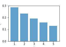
Figure 1: $P_{o}$ in the experiments carried out with the 1-parameter example model.

We used the model to simulate 1000 observation sets with $n_{o}=\{50,100,500,1000\}$ samples and calculated the proposed test statistics based on the observation sets and simulations with $n=n_{o}$ and $n=1000n_{o}$ samples.

We start with experiments where the proposed test statistic values are calculated with $E_{P_{\theta}}\left[D_{\rm JS,1/2}(\widehat{P}_{\mathbf{D}},\widehat{Q}_{\theta})\right]$ estimated based on $m=1000$ simulations carried out with the true parameter value. A visual comparison between the expected null distribution and observed test statistic values indicates a reasonable fit in all test conditions (Figure 2).

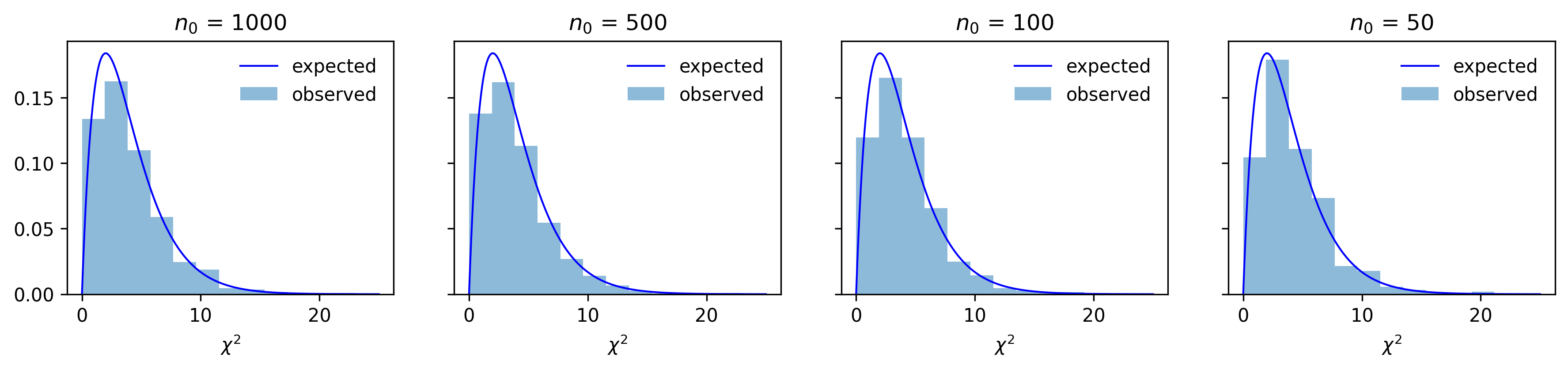
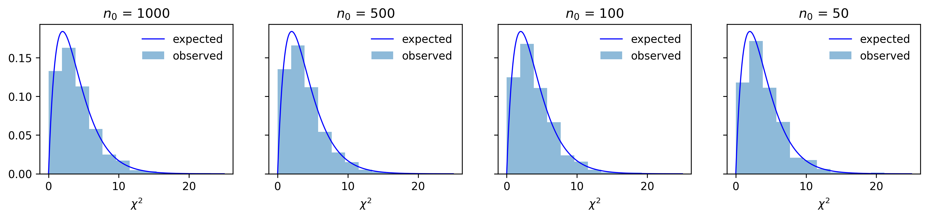
(a) (b) (c)

Figure 2: The expected asymptotic distribution and test statistics calculated based on observations simulated with 1-parameter example model. The proposed test statistic values were calculated based on $m=1000$ simulations with (a) $n=n_{o}$ or (b) $n=1000n_{o}$ samples. For comparison, see (c) Pearson statistics calculated based on the true category probabilities.

This is confirmed when we examine the coverage probabilities presented in Figure 3.

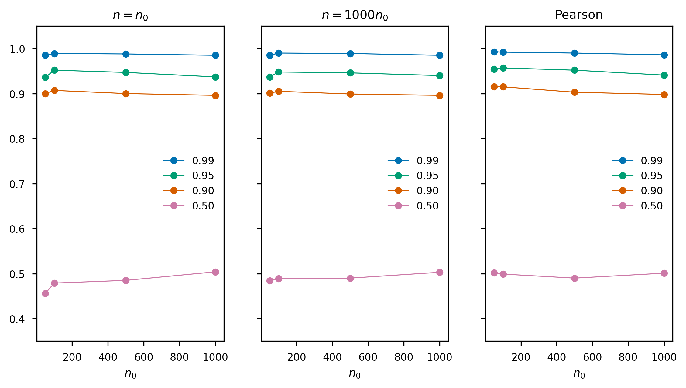
Figure 3: Coverage probabilities calculated based on observations simulated with the 1-parameter example model. The proposed test statistic values were calculated based $m=1000$ simulations with $n=n_{o}$ or $n=1000n_{o}$ samples. Coverage probabilities calculated with the Pearson statistic are presented for comparison.

We observe that the coverage probabilities are close to the nominal value $1-\alpha$ in all test conditions, and while the coverage probabilities are lower than the nominal value in some conditions when the observed and simulated sample are small, the coverage probabilities in all test conditions converge to the nominal values when $n_{o}$ increases.

We then proceed to evaluate test statistics calculated based on $E_{P_{\theta}}\left[D_{\rm JS,1/2}(\widehat{P}_{\mathbf{D}},\widehat{Q}_{\theta})\right]$ estimated using the surrogate model in BO. BO was initialized with 20 simulations and the total simulation count was set to 1000. The parameter values included in the initialization set were selected at random within $[-1,1]$ and optimization was carried out in this range. The coverage probabilities calculated based on the proposed test statistic are presented in Figure 4.

Figure 4: Coverage probabilities calculated based on observations simulated with the 1-parameter example model when the test statistics were calculated based on the BOLFI model using simulations with $n=n_{o}$ or $n=1000n_{o}$ samples.

The coverage probabilities are close to $1-\alpha$ in all test conditions, but in contrast to the results presented in Figure 3, do not converge to the nominal value when $n_{o}$ increases if $n=n_{o}$. This because the $E_{P_{\theta}}\left[D_{\rm JS,1/2}(\widehat{P}_{\mathbf{D}},\widehat{Q}_{\theta})\right]$ calculated based on the surrogate model is not as accurate as the estimate calculated based on $m=1000$ simulations, and while the estimates become more accurate when $n$ increases and there is less variation between simulations, the estimation errors are multiplied with $n_{o}$ when we calculate the test statistic, meaning that an increase in sample size may not decrease the error in test statistic values when $n=n_{o}$ (Figure 5).

(a) (b)

Figure 5: Estimation errors calculated as difference between (a) simulator-based JSD and (b) test statistic values calculated based on the BOLFI model or $m=1000$ simulations.

While using a surrogate model can introduce estimation error in the test statistic values, it has the benefit that we can test large candidate sets without additional simulation cost. Figure 6 shows coverage probabilities calculated with respect to the model parameter $\theta$.

(a) (b)

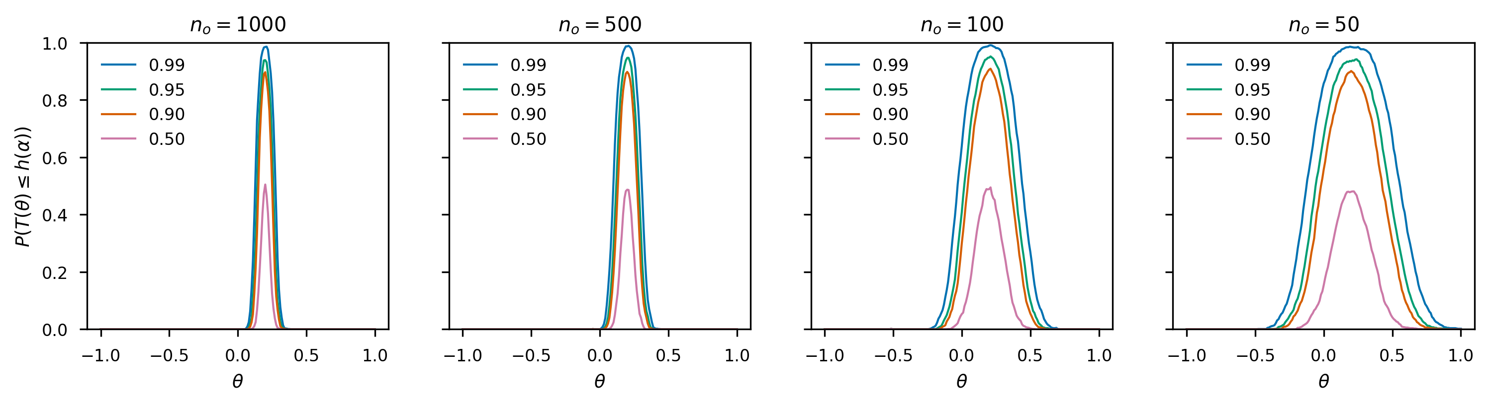
Figure 6: Proportion of confidence intervals that include the parameter value $\theta$ when observations were generated with the 1-parameter example model using $\theta=0.2$ and the proposed test statistic values were calculated based on the BOLFI model using simulations with (a) $n=n_{o}$ or (b) $n=1000n_{o}$ samples.

We see that the confidence intervals estimated based on the proposed test statistic are expected to cover a range around the true parameter value, and that the range becomes wider when we reduce the observed data set size $n_{o}$.

10.4 Experiment 2

The second experiments are carried out with the standard log-linear model that is used to describe association and interaction patterns between two categorical random variables. Here we model the counts in a two-way table as a sample from a multinomial distribution with $k=4$ categories. The observation probabilities are calculated based on the normalized exponential function as

$$p_{i}(\theta)=\sigma(\log(\mu_{i}))=\sigma(\lambda+X_{i}\lambda^{X}+Y_{i}\lambda^{Y}+X_{i}Y_{i}\lambda^{XY}),\quad i=1,2,3,4,$$ (102)

where $\sigma(z_{i})$ denotes the normalized exponential function output $\sigma(z_{i})=\exp(z_{i})/\sum_{i}\exp(z_{i})$, and $X_{i}$ and $Y_{i}$ are coded variable values and $\mu_{i}$ denote the expected observation counts. We assume effect-coded variables that take values 1 or -1 as indicated in Table 1.

$i$	1	2	3	4
$X_{i}$	1	1	-1	-1
$Y_{i}$	1	-1	1	-1

Table 1: Effect coding in the log-linear example.

The model parameters $\lambda^{X}$ and $\lambda^{Y}$ then encode expected difference in the proportion between 1 and -1 values in variables $X$ and $Y$, and the parameter $\lambda^{XY}$ encodes possible association between the two variable values. Finally the constant $\lambda$ is calculated based on the other parameter values and total count $n$ so that the sum over expected counts equals $n$.

We run experiments with two model versions. We use a two-parameter model where $\lambda^{XY}=0$ and the model parameters $\theta=(\lambda^{X},\lambda^{Y})$ and a saturated model where the model parameters $\theta=(\lambda^{X},\lambda^{Y},\lambda^{XY})$. The true parameter values are set to $\lambda^{X}=-0.25$ and $\lambda^{Y}=0.15$ in the two-parameter version and to $\lambda^{X}=-0.20$, $\lambda^{Y}=0.10$, and $\lambda^{XY}=0.40$ in the saturated three-parameter version. The corresponding category probabilities are visualized in Figure 7.

(a)	(b)

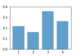
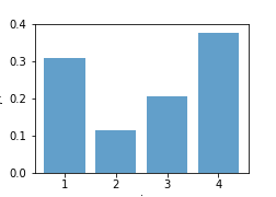
Figure 7: $P_{o}$ in the experiments carried out with the (a) 2-parameter and (b) 3-parameter log-linear model.

Both model versions were used to simulate 1000 observation sets with $n_{o}=\{50,100,500,1000\}$ samples.

We run the same experiments that were carried out with the 1-parameter example model studied in the previous section. We start with the proposed test statistics calculated based on $m=1000$ simulations carried out with the true parameter values with sample size $n=n_{o}$ and $n=1000n_{o}$. Figure 8 shows coverage probabilities calculated based on comparison between the observed test statistic values and the expected null distribution.

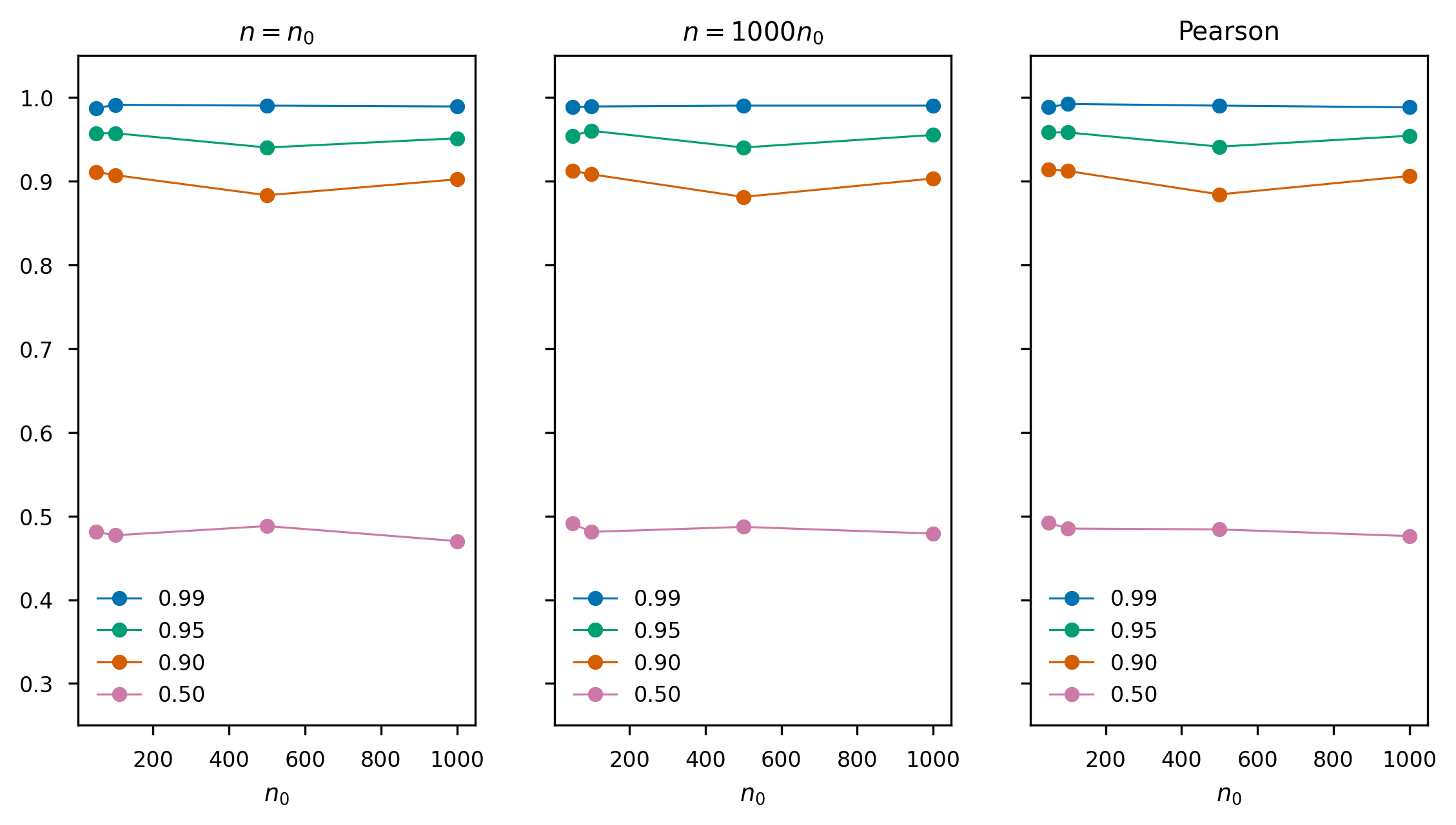
(a) (b)

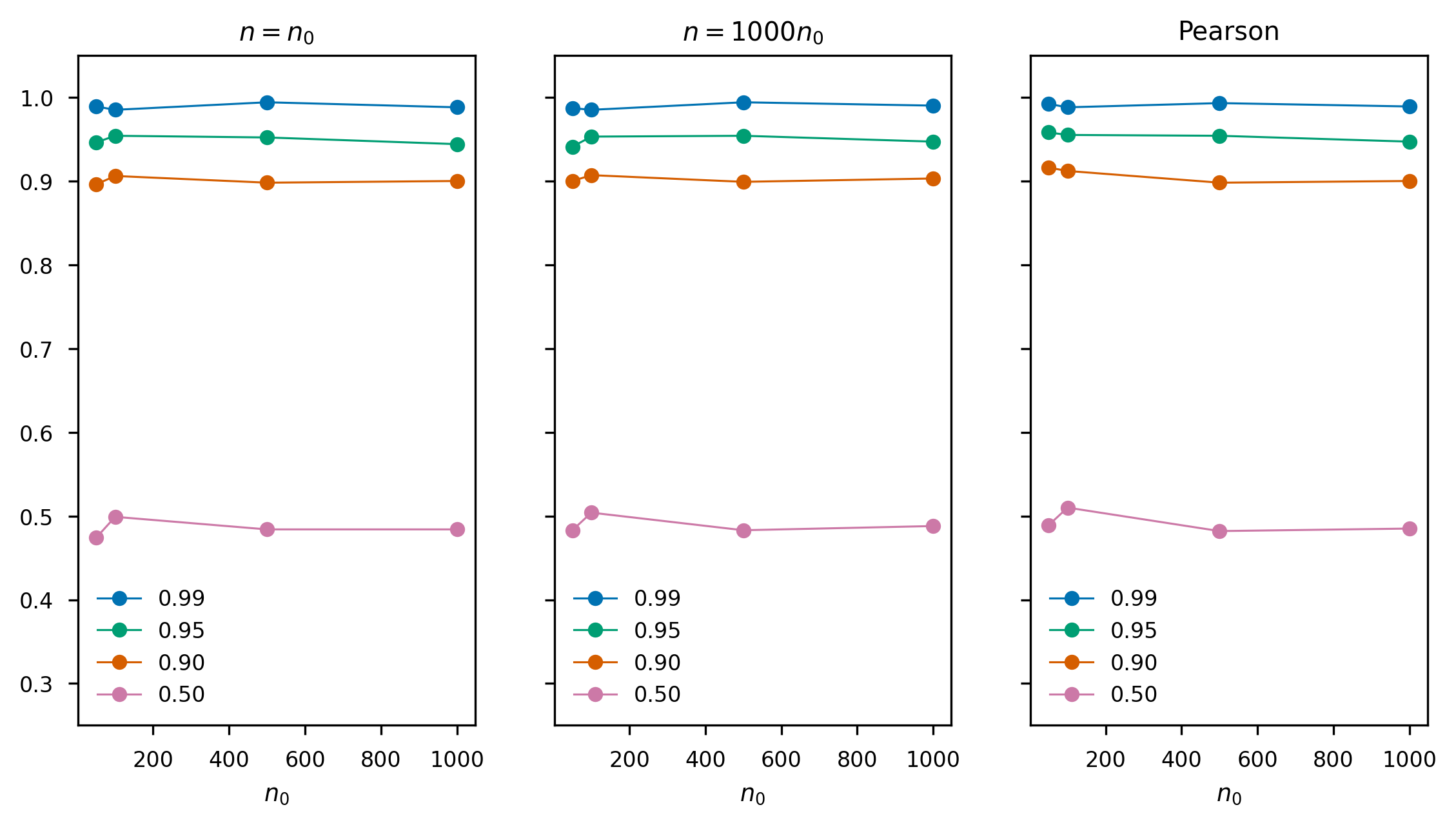
Figure 8: Coverage probabilities calculated based on observations simulated with the (a) 2-parameter or (b) 3-parameter log-linear model. The proposed test statistic values were calculated based $m=1000$ simulations with $n=n_{o}$ or $n=1000n_{o}$ samples. Coverage probabilities calculated with the Pearson statistic are presented for comparison.

The coverage probabilities calculated based on the proposed test statistic follow the coverage probabilities calculated with the Pearson statistic and are close to the nominal value $1-\alpha$ in all test conditions.

We also evaluate the proposed test statistic values calculated based on the surrogate model in BO. In this experiment we initialized BO with 50 simulations and set the total simulation count to 2000. The parameter values included in the initialization set were selected at random within $[-1,1]$ and optimization was carried out in this range. Coverage probabilities calculated based on the proposed test statistic are visualized in Figure 9.

(a)

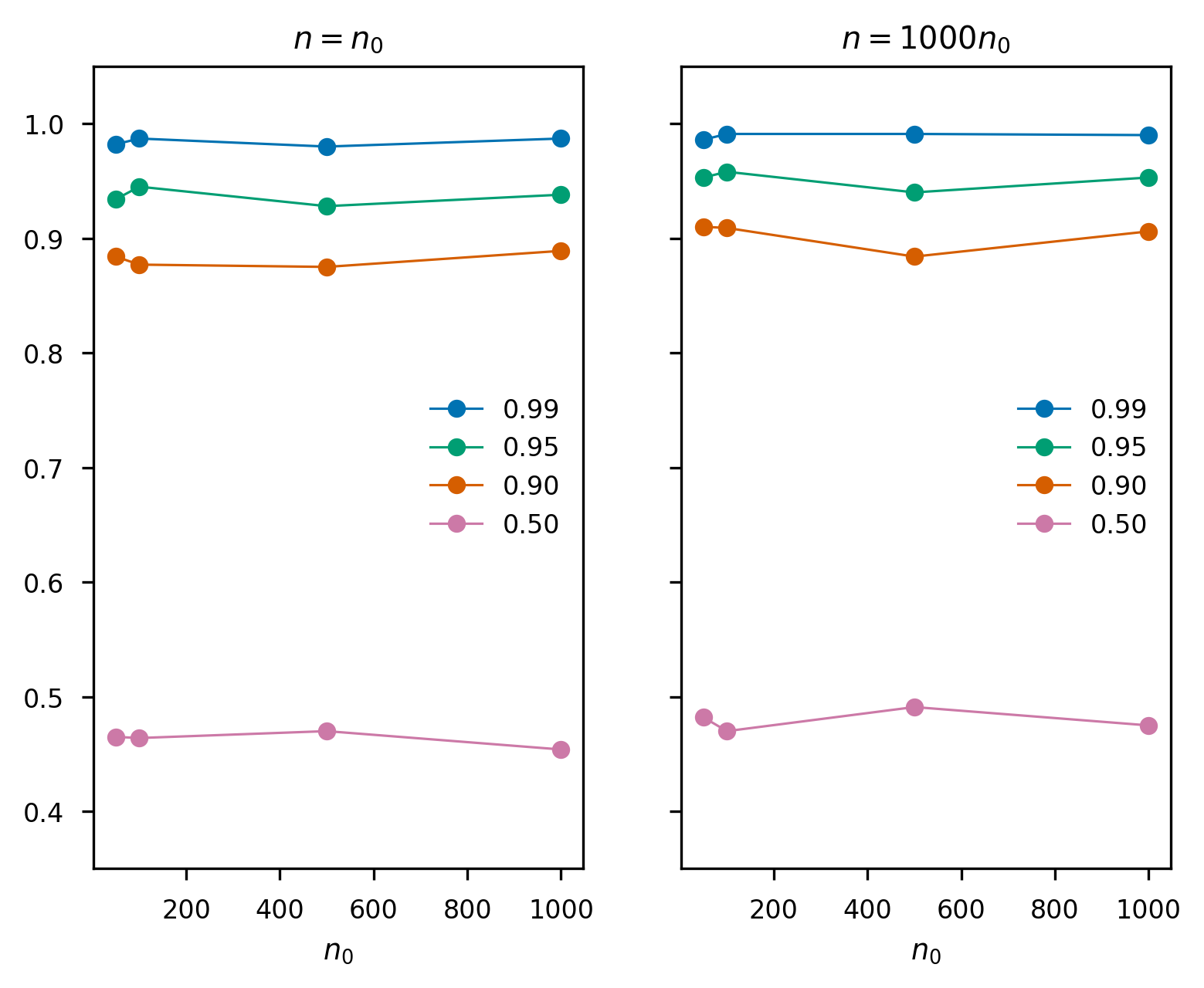
(b)

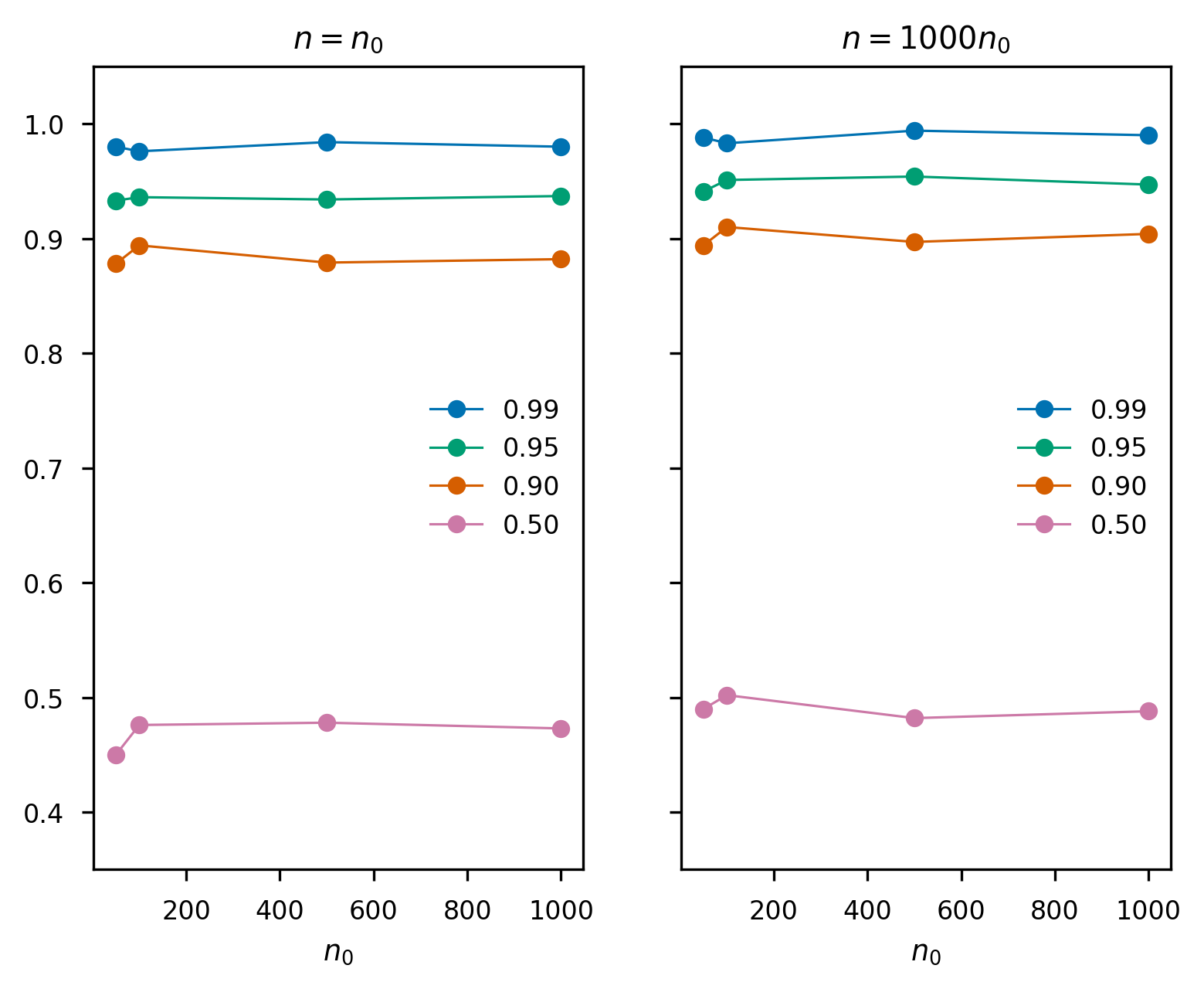
Figure 9: Coverage probabilities calculated based on observations simulated with the (a) 2-parameter or (b) 3-parameter log-linear model when the test statistics were calculated based on the BOLFI model using simulations with $n=n_{o}$ or $n=1000n_{o}$ samples.

We observe that the coverage are close to the nominal value in all test conditions, but do not converge to $1-\alpha$ when $n_{o}$ increases if $n=n_{o}$.

10.5 Experiment 3

The last experiment is carried out with a model that simulates the evolution of genotype frequencies. Corander et al. (2017) used the model to capture non-negative frequency dependent selection (NFDS) in the post-vaccine evolution of pneumococcal populations. The simulator code is available online and the present experiments are carried out with the model version that simulates homogeneous-rate multilocus NFDS. Evolution is modeled as a discrete-time process where the population at time $t+1$ is sampled with replacement from the population at time $t$ with observation counts

$$X_{i,t}\sim\mathrm{Poisson}\left(\frac{\kappa}{N_{t}}(1-m)(1-v_{i})(1+\sigma_{f})^{\pi_{i,t}}\right),$$ (103)

where $i$ indexes the isolates in population at time $t$. The first term accounts for general density-dependent selection where $\kappa$ denotes the carrying capacity and $N_{t}$ is the population size at time $t$. In the current experiment we assumed $\kappa=10^{5}$. The second term with migration rate $m$ models the pressure from migration into the population. The third term describes negative selection pressure due to the vaccine: $v_{i}=v$ if the isolate $i$ has vaccine serotype and zero otherwise. Finally the last term describes the positive selection pressure associated with rare alleles under NFDS: $\pi_{i,t}$ measures the deviation between isolate $i$ and the equilibrium genotype at time $t$, and the selection pressure is modeled with parameter $\sigma_{f}$. Parameter estimation is carried out in the log-compressed parameter domain with $\theta=(\ln(m),\ln(v),\ln(\sigma_{f}))$.

We use the model to simulate 1000 observation sets that are modeled on pneumococcal data studied by Corander et al. (2017). The data set studied in previous work includes a pre-vaccination ($t=0$) sample with 133 isolates and two post-vaccination samples with 203 isolates collected at $t=36$ and 280 isolates collected at $t=72$ (Croucher et al., 2013). We use this data to create the simulated observation sets as follows. We sample the pre-vaccination data to initialize the simulated population at $t=0$, simulate how the population evolves under selected model parameters, and then sample the simulated population at $t=36$ and $t=72$ to create simulated post-vaccination samples with $n_{o}=250$ or $n_{o}=1000$ isolates. The parameter values used in the simulations were $\ln(m)=-5.3$, $\ln(v)=-2.5$, and $\ln(\sigma_{f})=-5.3$.

The isolates in the simulated observation sets are arranged into 41 sequence clusters based on genetic content and typed as vaccine type (VT) or non-vaccine type (NVT) (Corander et al., 2017). This creates $k=82$ potential observation categories. However some sequence clusters are exclusive to vaccine or non-vaccine types, which means that some categories are never observed. To remove these categories, and to ensure that all categories have adequate observation counts, we collapsed the data into $k=4$ observation categories as follows: $i=1$ includes all VT isolates while $i=2$ includes NVT isolates in sequence clusters that do not include VT isolates at $t=0$, $i=3$ includes NVT isolates in sequence clusters that include VT isolates at $t=0$, and $i=4$ includes NVT isolates in sequence clusters that are not present in the observed data at $t=0$. The negative selection pressure due to vaccine should then be observed as a decrease in category 1, while migration and NFDS control the balance between categories 2–4. This is observed in the average category proportions calculated based on the simulated observations sets used in this experiment (Figure 10).

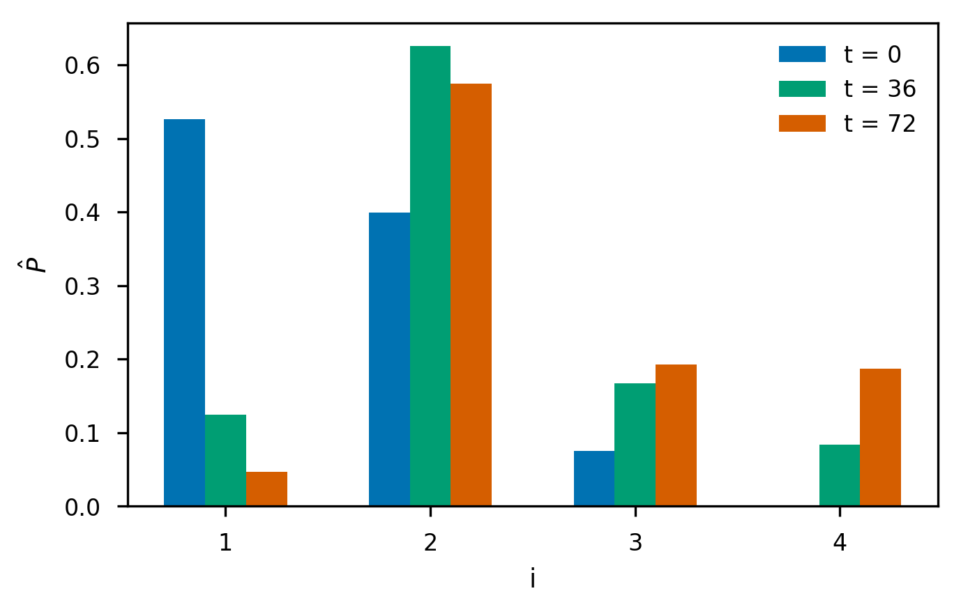
Figure 10: Average category proportions calculated based on 1000 observation sets simulated with the NFDS model.

To summarize, we simulated 1000 observation sets by sampling simulated populations at $t=36$ and $t=72$ and divided the isolates in each sample into $k=4$ observation categories. These are compared to simulated data based on a discrepancy measure calculated as the sum over JSD between the data collected at $t=36$ and JSD between the data collected at $t=72$. We calculate the expected discrepancy based on repeated simulations or a BOLFI model, and use it to calculate test statistic values that correspond to the sum over proposed test statistic values calculated based on expected JSD at $t=36$ and $t=72$.

We start with the proposed test statistic values calculated based on $m=1000$ simulations carried out with the true parameter values and $n=n_{o}$. The expected and observed distributions are compared in Figure 11 (a) and coverage probabilities reported in Table 2 (a).

(a)

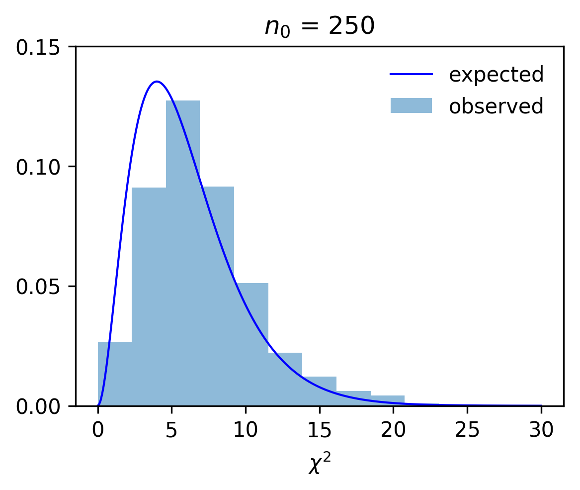
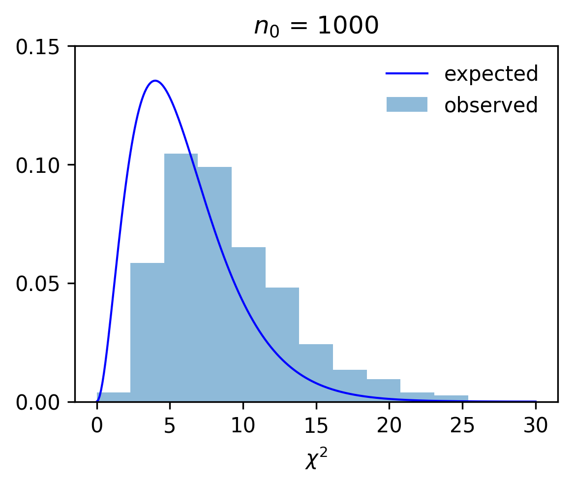
(b)

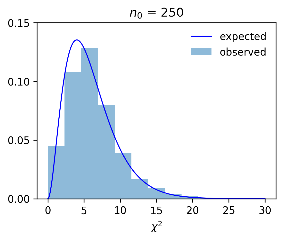
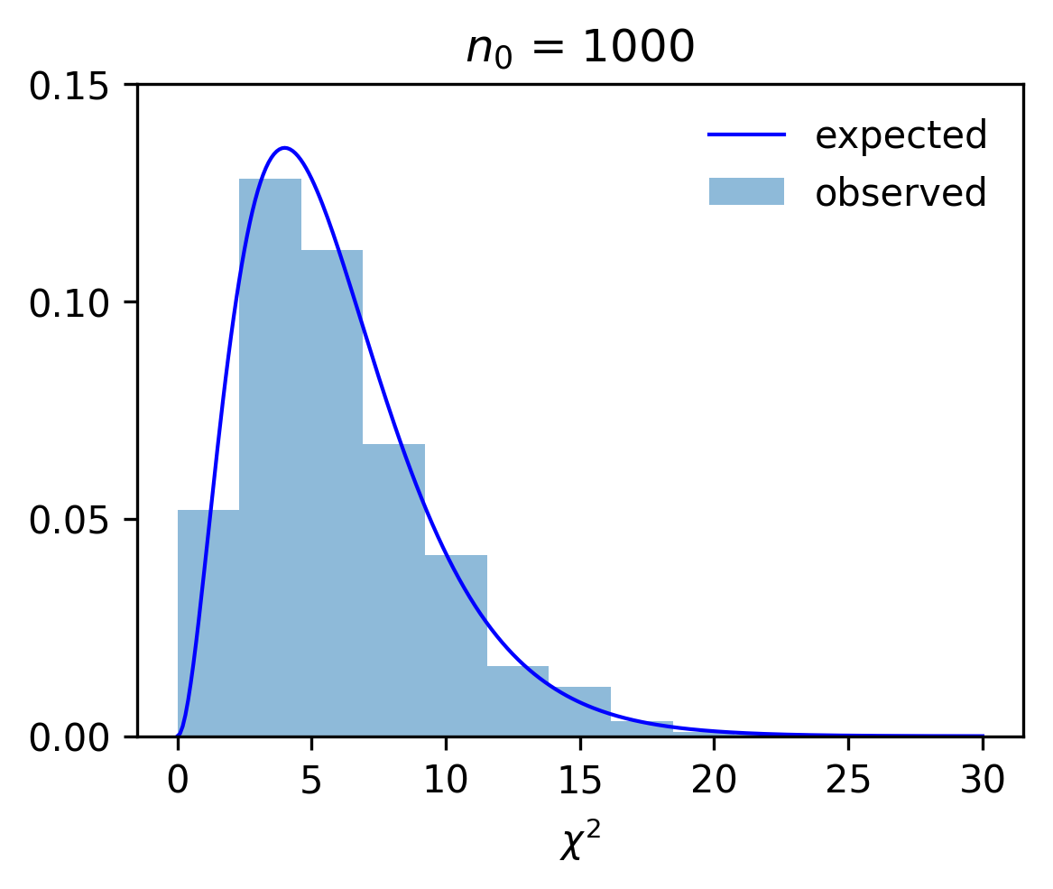
Figure 11: The expected asymptotic distribution and test statistics calculated based on observations simulated with the NFDS model. The proposed test statistic values were calculated based on $m=1000$ simulations with $n=n_{o}$ and based on sample size (a) $n_{o}$ or (b) ESS.

(a)

$1-\alpha$ $n_{o}=250$ $n_{o}=1000$ 0.99 0.98 0.94 0.95 0.93 0.82 0.90 0.86 0.71 0.50 0.36 0.22

(b)

$1-\alpha$ $n_{o}=250$ $n_{o}=1000$ 0.99 0.99 0.99 0.95 0.94 0.94 0.90 0.90 0.90 0.50 0.46 0.51

Table 2: Coverage probabilities calculated based on observations simulated with the NFDS model. The proposed test statistic values were calculated based on $m=1000$ simulations with $n=n_{o}$ and based on sample size (a) $n_{o}$ or (b) ESS.

We observe that the test statistic values are overestimated compared to the expected null distribution, and the coverage probabilities are lower than the nominal value. This is because the observations in this example exhibit more variation than a multinomial sample with the same size. The additional variation also does not depend on the sample size, which means that the error between observed and expected test statistic distribution increases when the sample size increases and less variation is expected. However we can use the simulated data to estimate ESS that compensates for the overdispersion. When the proposed test statistic is calculated based on ESS, the observed distribution follows the expected distribution well (Figure 11 (b)) and the coverage probabilities are close to the nominal value $1-\alpha$ in all test conditions (Table 2 (b)). The average ESS was 236 when $n_{o}=250$ and 806 when $n_{o}=1000$ (Figure 12).

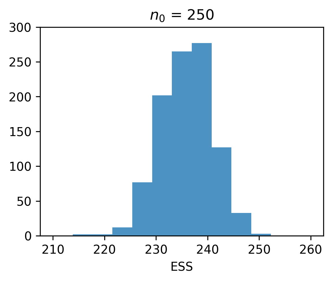
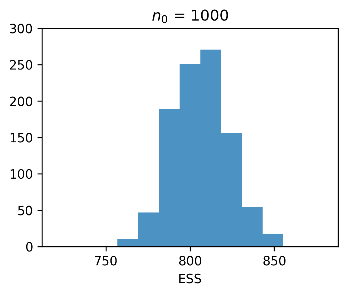
Figure 12: Effective sample size calculated based on the $m=1000$ simulations carried out with the true simulator parameters.

We also evaluate the proposed test statistic calculated based on the surrogate model in BO. The parameter ranges considered in optimization were $\ln(m)\in[-7,-1.6]$, $\ln(v)\in[-7,-0.7]$, and $\ln(\sigma_{f})\in[-7,-1.6]$. We initialized optimization with 50 simulations and set the total simulation count to 2000. The additional variation observed in this example is expected to have some dependence on the model parameters, but since the parameters that could be included in a confidence set are close to the parameters $\hat{\theta}$ that minimize the expected simulator-based JSD, we approximate ESS at all parameter values with an estimate calculated based on $m=1000$ simulations carried out with $\hat{\theta}$. The average ESS was 235 when $n_{o}=250$ and 800 when $n_{o}=1000$ (Figure 13).

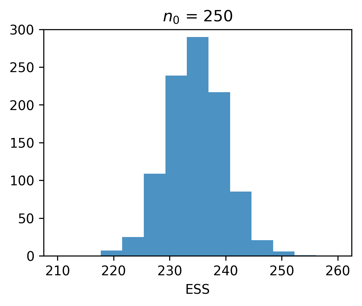
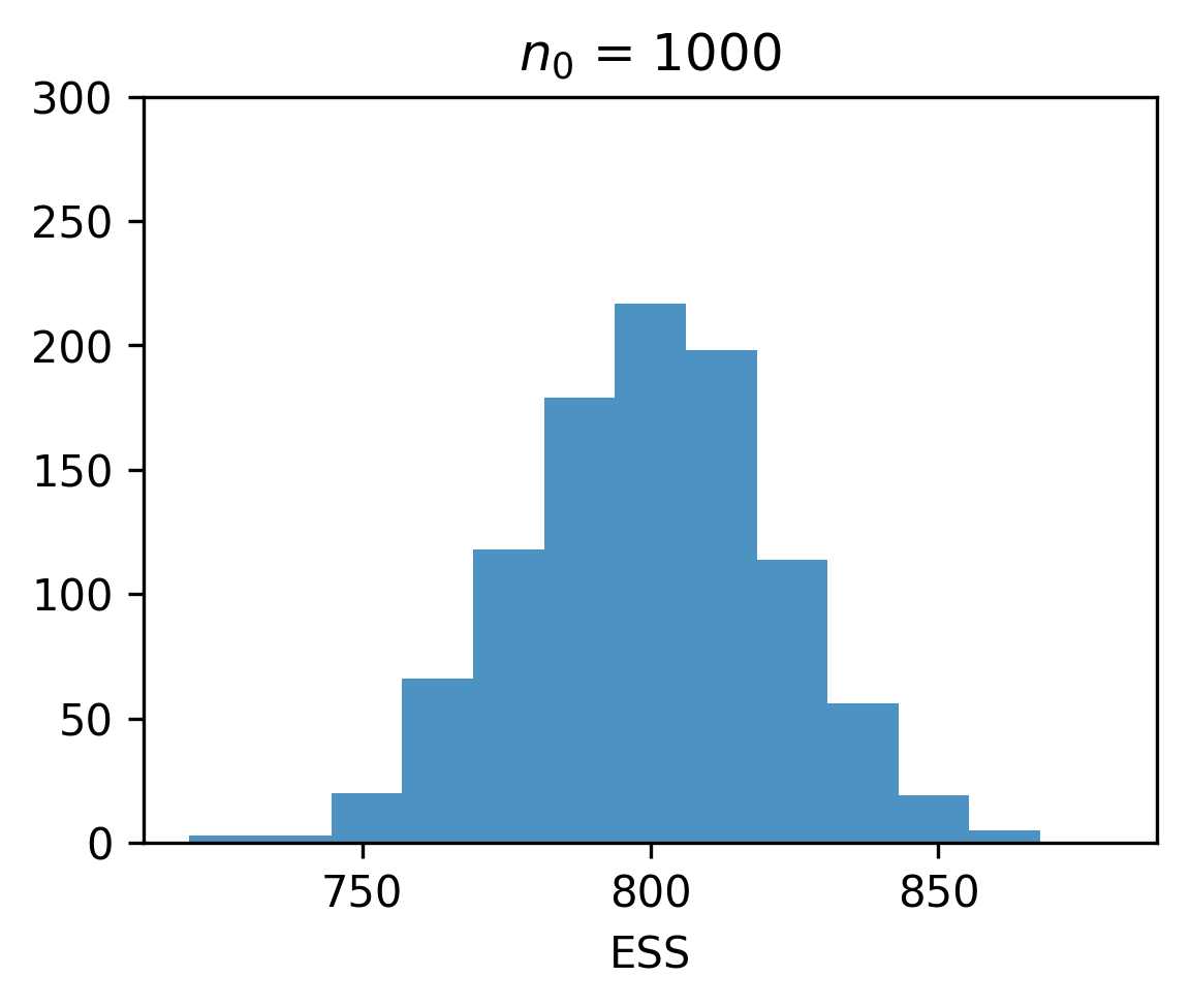
Figure 13: Effective sample size calculated based on $m=1000$ simulations carried out with the parameters that minimize the expected JSD between observed and simulated data.

Coverage probabilities calculated based on the proposed test statistic are reported in Table 3.

(a)

$1-\alpha$ $n_{o}=250$ $n_{o}=1000$ 0.99 0.96 0.73 0.95 0.86 0.58 0.90 0.75 0.48 0.50 0.28 0.16

(b)

$1-\alpha$ $n_{o}=250$ $n_{o}=1000$ 0.99 0.98 0.86 0.95 0.89 0.75 0.90 0.82 0.67 0.50 0.35 0.32

Table 3: Coverage probabilities calculated based on observations simulated with the NFDS model. The proposed test statistic values were calculated based on the BOLFI model using simulations with $n=n_{o}$ and based on sample size (a) $n_{o}$ or (b) ESS.

We observe that the coverage probabilities are lower than the corresponding coverage probabilities reported in Table 2. This is due to overestimation errors introduced in BOLFI (Figure 14).

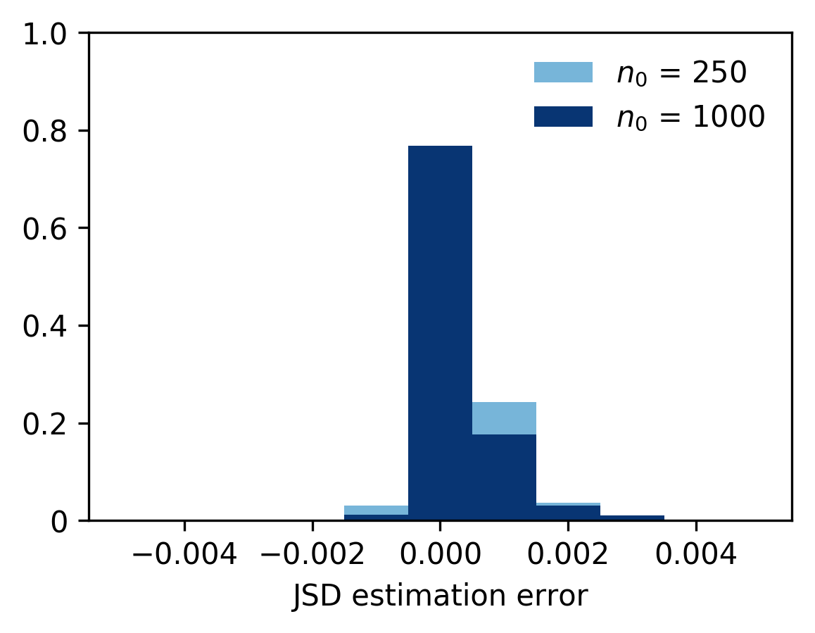
Figure 14: Estimation errors calculated as difference between the average over simulator-based JSD evaluated at $t=36$ and $t=72$ calculated based on the BOLFI model or $m=1000$ simulations.

11 Discussion and conclusions

Despite some early interest in the frequentist likelihood-free inference, more recently the primary focus of the research has been on approximating the posterior distribution of parameters with various sampling and surrogate model based approaches. As these methods can be very computation intensive and/or do require considerable expertise about training surrogate models, there is a clear need for further research on alternative approaches that would exploit asymptotic behavior of the approximate implicit likelihood. In the present work we considered this objective for the situation where the Jensen–Shannon divergence between observed and simulated data is used to measure the model fit and find model parameters that best explain the observed data. We derived explicit expressions for the expectation and variance of the simulator-based JSD statistic (Section 7) and proposed a test statistic that can be used in hypothesis testing or confidence set estimation (Section 8–9).

We carried out simulation experiments to evaluate the proposed test statistic and to examine whether test statistic values can be calculated based on the surrogate model in BOLFI. The coverage probabilities reported in Sections 10.3 and 10.4 indicate that the test statistic values follow the expected asymptotic distribution when the sample size is large and the observed and simulated data follow a multinomial distribution. The experiments thus confirmed that the proposed approach can be used to evaluate parameter fit and calculate confidence sets in such conditions. Meanwhile experiments carried out with the NFDS model (Section 10.5) showed that the test statistic can be sensitive to the multinomial distribution assumption. While this is a concern when we want to use the test statistic with simulator-based models, the experiments also showed that substituting sample size with ESS can compensate for deviations caused by extra heterogeneity in data. In addition the example demonstrated collapsing observation categories to ensure adequate observation count in all categories.

The BOLFI experiments indicated that the proposed test statistic is sensitive to errors in the estimated JSD value. Experiments carried out with the multinomial example models suggested that the estimation error is related to variation between simulated data sets. Since the variation in this case depended on the simulated sample size, using simulated samples that are larger than the observed sample allowed accurate test statistic calculation in these examples. However increasing the simulated sample size is not expected work when the variation has other sources. Hence rather than assume that the variation can be removed, we need to improve how variation between simulator-based JSD values is modelled in BOLFI.

While the current work is solely focused on the properties of JSD-based inference for models where the output can be summarized in terms of categorical distributions, there are multiple possible venues of future research to expand applicability of the theory. For example, quantization of continuous distributions can be used to enable application of JSD to more general model classes. An interesting question is then how the loss of information will depend on the chosen quantization and how accurate inference statements could be made about the model parameters as the sample size grows. In summary, we anticipate that a rich theory and applications can be found for more analytically oriented likelihood-free inference, where approximate likelihood quantities can be combined with efficient optimization algorithms.

A Asymptotics

A.1 An Auxiliary Bound for $D_{\rm JS}(P,Q)$

The following bound is included to make the argument below more self-contained.

Lemma A.1

$P\in\mathbb{P}$, $Q\in\mathbb{P}$. Assume $V(P,Q)<1/2$. Then

$$D_{\rm JS}(P,Q)\leq-\pi(1-\pi)\ln\left(\pi(1-\pi)\right)V(P,Q)-2\pi(1-\pi)V(P,Q)\ln\left(\frac{V(P,Q)}{k}\right).$$ (A.1)

Proof : We have from Equation (27)

$$D_{\rm JS}(P,Q)=\pi\left(H(M)-H(P)\right)+(1-\pi)\left(H(M)-H(Q)\right)$$

and then, since $D_{\rm JS}(P,Q)=\mid D_{\rm JS}(P,Q)\mid$,

$$D_{\rm JS}(P,Q)\leq\pi\left|H(M)-H(P)\right|+(1-\pi)\left|H(M)-H(Q)\right|.$$

By definition

$$V(M,P)=\sum_{i=1}^{k}|(\pi p_{i}+(1-\pi)q_{i})-p_{i}|$$

$$=\sum_{i=1}^{k}|(1-\pi)q_{i}-(1-\pi)p_{i}|=(1-\pi)V(Q,P)=(1-\pi)V(P,Q),$$

and similarly $V(M,Q)=\pi V(P,Q)$. For $\pi\in[0,1]$ $(1-\pi)V(P,Q)\leq V(P,Q)$ and $(1-\pi)V(P,Q)\leq V(P,Q)$, we get by assumption that $V(M,P)<\frac{1}{2}$ and $V(M,Q)<\frac{1}{2}$. Hence by Lemma 2

$$\pi\left|H(M)-H(P)\right|\leq-\pi(1-\pi)V(P,Q)\cdot\ln\left(\frac{(1-\pi)V(P,Q)}{k}\right)$$

and

$$(1-\pi)\left|H(M)-H(Q)\right|\leq-\pi(1-\pi)V(P,Q)\cdot\ln\left(\frac{\pi V(P,Q)}{k}\right).$$

This gives

$$\pi\left|H(M)-H(P)\right|+(1-\pi)\left|H(M)-H(Q)\right|\leq-\pi(1-\pi)V(P,Q)\ln\left(\frac{\pi(1-\pi)V(P,Q)^{2}}{k^{2}}\right).$$

Hence the bound in Equation (28) follows, as claimed.  
For $\pi=\frac{1}{2}$ the upper bound in Equation (28) assumes its smallest value and the bound becomes

$$D_{\rm JS}(P,Q)\leq\frac{1}{2}V(P,Q)\left[\ln 2-\ln\left(\frac{V(P,Q)}{k}\right)\right].$$ (A.2)

As $k\geq 2$ and $V(P,Q)\leq 2$, we have $1\geq V(P,Q)/k$. Hence the bound in Equation (A.1) is less sharp than the bound $D_{\rm JS}(P,Q)\leq\frac{\ln 2}{2}V(P,Q)$ in (Corander et al., 2021, Equation (20), p.885) valid for any $V$ and $\pi\in(0,1)$, but suffices for the present purposes.

A.2 $V\left(\widehat{Q}_{\theta},P_{\theta}\right)\rightarrow 0$

Lemma A.2

$\widehat{Q_{\theta}}\in\mathbb{M}_{n}(\theta)$.

$$V\left(\widehat{Q}_{\theta},P_{\theta}\right)\rightarrow 0,\mbox{as $n\rightarrow+\infty$}$$ (A.3)

$P_{\theta}$-a.s..

Proof  By definition, $V\left(\widehat{Q}_{\theta},P_{\theta}\right)=\sum_{i=1}^{k}\left|\frac{\xi_{i}}{n}-p_{i}(\theta)\right|$. We bound for any $\epsilon>0$

$$P_{\theta}\left(\sum_{i=1}^{k}\left|\frac{\xi_{i}}{n}-p_{i}(\theta)\right|\geq\epsilon\right)=P_{\theta}\left(\sum_{i=1}^{k}\left|\xi_{i}-np_{i}(\theta)\right|\geq n\epsilon\right).$$

If the event $n\epsilon\leq\sum_{i=1}^{k}\left|\xi_{i}-np_{i}(\theta)\right|$ occurs, there is at least one $|\xi_{i}-np_{i}(\theta)|\geq\frac{n\epsilon}{k}$. Thus we bound upwards by the union bound

$$\leq P_{\theta}\left(\cup_{i=1}^{k}\left\{\left|\xi_{i}-np_{i}(\theta)\right|\geq\frac{n\epsilon}{k}\right\}\right)\leq\sum_{i=1}^{k}P_{\theta}\left(\left|\xi_{i}-np_{i}(\theta)\right|\geq\frac{n\epsilon}{k}\right).$$

Here $\xi_{i}\sim{\rm Bin}(n,p_{i}(\theta))$, $\xi_{i}$ is a sum of $n$ i.i.d. Bernoulli r.v.s and the mean of the sum is $np_{i}(\theta)$. The Hoeffding inequality (Devroye et al., 2013, Thm 8.1) gives

$$P_{\theta}\left(\left|\xi_{i}-np_{i}(\theta)\right|\geq\frac{n\epsilon}{k}\right)\leq 2e^{-2n\epsilon^{2}/k^{3}}.$$

Hence

$$\sum_{i=1}^{k}P_{\theta}\left(\left|\xi_{i}-np_{i}(\theta)\right|\geq\frac{n\epsilon}{k}\right)\leq 2ke^{-2n\epsilon^{2}/k^{3}}$$

and by the preceding chain of inequalities

$$\sum_{n=1}^{+\infty}P_{\theta}\left(\sum_{i=1}^{k}\left|\frac{\xi_{i}}{n}-p_{i}(\theta)\right|\geq\epsilon\right)<+\infty,$$

and Equation (A.3) follows by the Borel-Cantelli lemma.  
The proof above implements the hint of proof for the case at hand in Berend and Kontorovich (2012). The proof shows in fact complete convergence, see e.g., Gut (2013, p.203). In addition, ${\mathbf{D}}=(D_{1},\ldots,D_{n_{o}})$, an i.i.d. $n_{o}$-sample $\sim$ $P_{o}$ with $\widehat{P}_{\mathbf{D}}$ that

$$V\left(\widehat{P}_{\mathbf{D}},P_{o}\right)\rightarrow 0,\mbox{as $n_{o}\rightarrow+\infty$}$$ (A.4)

$P_{o}$-a.s.. We get the following statement.

Theorem A.3

$\widehat{Q_{\theta}}\in\mathbb{M}_{n}(\theta)$.

$$D_{\rm JS}\left(\widehat{Q}_{\theta},P_{\theta}\right)\rightarrow 0,\mbox{as $n\rightarrow+\infty$}$$ (A.5)

$P_{\theta}$-a.s..

Proof : By Equation (A.4) there exists $n_{1/2}$ such that $V\left(\widehat{Q}_{\theta},P_{\theta}\right)<1/2$ for all $n>n_{1/2}$ with probability one. Hence Lemma A.1, i.e., Equation (A.1), entails that $D_{\rm JS}\left(\widehat{Q}_{\theta},P_{\theta}\right)\rightarrow 0$, as $n\rightarrow+\infty$, since $V\ln V\rightarrow 0$, when $V\rightarrow 0$.  

A.3 Further Asymptotics of KLD and Variation Distance

Lemma A.4

(i)

Assume ${\rm supp}\left(P_{\theta}\right)={\cal A}$ and $\widehat{Q}_{\theta}\in\mathbb{M}_{n}(\theta)$. Then, as $n\rightarrow+\infty$

$$D_{\rm KL}\left(\widehat{Q}_{\theta},P_{\theta}\right)\rightarrow 0,$$ (A.6)

$P_{\theta}$- a.s..

(ii)

Assume ${\rm supp}\left(P_{\theta_{o}}\right)={\cal A}$. ${\mathbf{D}}=(D_{1},\ldots,D_{n_{o}})$, is an i.i.d. $n_{o}$-sample $\sim$ $P_{\theta_{o}}$. Then, as $n_{o}\rightarrow+\infty$

$$D_{\rm KL}\left(\widehat{P}_{\mathbf{D}},P_{\theta_{o}}\right)\rightarrow 0,$$ (A.7)

$P_{o}$-a.s..

Proof  The assertions $\bf(i)$ and $\bf(ii)$ follow respectively from Equations (A.3) and (A.4) by the reverse Pinsker inequality for $P\in\mathbb{P}$ and $Q\in\mathbb{P}$, and $Q_{min}=\min_{1\leq j\leq k}q_{j}$,

$$D_{\rm KL}(P,Q)\leq\frac{1}{Q_{min}}V(P,Q)^{2}.$$ (A.8)

In $\bf(i)$ take $P=\widehat{Q}_{\theta}$ and $Q=P_{\theta}$ and analogously for $\bf(ii)$. Note that $V(P,Q)=V(Q,P)$.  
For the reverse Pinsker inequality, see Sason (2015), and Sason and Verdú (2016). The results in the corollary are known, see Cover and Thomas (2012, Thm 11.2.1), but are here justified by the reverse Pinsker inequality.

A.4 Asymptotics for Increasing ${\mathbf{D}}$

The convergence in Equation (A.6) of Lemma A.4 requires that there is a $\theta_{o}$ in the parameter space of the model such that observed data $\mathbf{D}$ are $\sim P_{\theta_{o}}$. Next we find a convergence that does not require this assumption, but reduces to Equation (A.6), if $P_{o}\in\mathbb{M}$.

Lemma A.5

Assume that Equation (6) holds for $P_{o}\in\mathbb{P}$ and for any $P_{\theta}\in\mathbb{M}$. Let ${\mathbf{D}}=(D_{1},\ldots,D_{n_{o}})$ be an i.i.d. $n_{o}$-sample $\sim$ $P_{o}$. Then it holds that

$$\lim_{n_{o}\rightarrow+\infty}D_{\rm KL}\left(\widehat{P}_{\mathbf{D}},P_{\theta}\right)=D_{\rm KL}\left(P_{o},P_{\theta}\right).$$ (A.9)

$P_{o}$-a.s..

Proof  From Cover and Thomas (2012, Thm 11.1.2) we have the identity

$$\ln P_{\theta}(\mathbf{D})=-n_{o}H\left(\widehat{P}_{\mathbf{D}}\right)-n_{o}D_{\rm KL}\left(\widehat{P}_{\mathbf{D}},P_{\theta}\right).$$ (A.10)

By the same token the probability of $\mathbf{D}$ under $P_{o}$ is

$$\ln P_{o}(\mathbf{D})=-n_{o}H\left(\widehat{P}_{\mathbf{D}}\right)-n_{o}D_{\rm KL}\left(\widehat{P}_{\mathbf{D}},P_{o}\right).$$ (A.11)

If the entropy expression from Equation (A.10) is substituted in Equation (A.11) we get

$$\ln P_{o}(\mathbf{D})=\ln P_{\theta}(\mathbf{D})+n_{o}\left[D_{\rm KL}\left(\widehat{P}_{\mathbf{D}},P_{\theta}\right)-D_{\rm KL}\left(\widehat{P}_{\mathbf{D}},P_{o}\right)\right]$$

and then

$$\frac{1}{n_{o}}\ln\frac{P_{o}({\mathbf{D}})}{P_{\theta}({\mathbf{D}})}=D_{\rm KL}\left(\widehat{P}_{\mathbf{D}},P_{\theta}\right)-D_{\rm KL}\left(\widehat{P}_{\mathbf{D}},P_{o}\right).$$ (A.12)

In the left hand side we have by the strong law of large numbers, that as $n_{o}\rightarrow+\infty$

$$\frac{1}{n_{o}}\ln\frac{P_{o}({\mathbf{D}})}{P_{\theta}({\mathbf{D}})}=\frac{1}{n_{o}}\sum_{i=1}^{n}\ln\frac{P_{o}(D_{i})}{P_{\theta}(D_{i})}\rightarrow D_{\rm KL}\left(P_{o},P_{\theta}\right)$$

$P_{o}$-a.s.. By Equation (A.7) $D_{\rm KL}\left(\widehat{P}_{\mathbf{D}},P_{o}\right)\rightarrow 0$, $P_{o}$-a.s., as $n\rightarrow+\infty$. When we allow these limits in Equation (A.12), the assertion in Equation (A.9) is established.  

Now we give the proof of Proposition 6.

Proof  We use the calculation in Equation (33) to obtain

$$D_{\rm JS}\left(\widehat{P}_{\mathbf{D}},P_{\theta}\right)=\pi D_{\rm KL}\left(\widehat{P}_{\mathbf{D}},P_{\theta}\right)-D_{\rm KL}\left(\widehat{M}_{\rm sp},P_{\theta}\right),$$ (A.13)

where $\widehat{M}_{\rm sp}:=\pi\widehat{P}_{\mathbf{D}}+(1-\pi)P_{\theta}$. We prove first that

$$D_{\rm KL}\left(\widehat{M}_{\rm sp},P_{\theta}\right)\rightarrow D_{\rm KL}\left(M_{o},P_{\theta}\right),$$

where $M_{o}:=\pi P_{o}+(1-\pi)P_{\theta}$. We bound $\left|D_{\rm KL}\left(\widehat{M}_{\rm sp},P_{\theta}\right)-D_{\rm KL}\left(M_{o},P_{\theta}\right)\right|$ as follows. We have by definition of $D_{\rm KL}$

$$\left|D_{\rm KL}\left(\widehat{M}_{\rm sp},P_{\theta}\right)-D_{\rm KL}\left(M_{o},P_{\theta}\right)\right| \leq \left|H\left(\widehat{M}_{\rm sp}\right)-H\left(M_{o}\right)\right|$$

$$+ \left|\sum_{j=1}^{k}m_{j,{\rm sp}}\ln\frac{1}{p_{j}\left(\theta\right)}-\sum_{j=1}^{k}m_{j,o}\ln\frac{1}{p_{j}\left(\theta\right)}\right|,$$

where we used Equation (6). But from this inequality on the proof of Theorem 5 shows that the convergence sought for here depends on the variation distance between $\widehat{M}_{\rm sp}$ and $M_{o}$. We have

$$V\left(\widehat{M}_{\rm sp},M_{o}\right)=\pi V\left(\widehat{P}_{\mathbf{D}},P_{o}\right).$$

By the remark in Equation (A.4) we see that $V\left(\widehat{P}_{\mathbf{D}},P_{o}\right)\rightarrow 0$, as $n_{o}\rightarrow+\infty$. Hence it follows as in the proof of Theorem 5 that

$$\left|D_{\rm KL}\left(\widehat{M}_{\rm sp},P_{\theta}\right)-D_{\rm KL}\left(M_{o},P_{\theta}\right)\right|\rightarrow 0,$$ (A.15)

$P_{o}$-a.s., as $n_{o}\rightarrow+\infty$. Now Equation (A.9) in Lemma A.5 and Equation (A.15) imply via Equation (A.13) that

$$D_{\rm JS}\left(\widehat{P}_{\mathbf{D}},P_{\theta}\right)\rightarrow\pi D_{\rm KL}\left(P_{o},P_{\theta}\right)-D_{\rm KL}\left(M_{o},P_{\theta}\right)$$ (A.16)

$P_{o}$-a.s., as $n_{o}\rightarrow+\infty$. But the calculus underlying Equation (A.13) verifies that the right hand side of Equation (A.16) equals $D_{\rm JS}\left(P_{o},P_{\theta}\right)$, as claimed.  
The next result is written in terms of the symmetric JSD with $\pi=1/2$, i.e., $D_{\rm JS,1/2}$, but the results hold obviously for any $\pi\in(0,1)$.

Proposition A.6

Assume that Equation (6) holds for $P_{o}\in\mathbb{P}$ and for any $P_{\theta}\in\mathbb{M}_{p}$. Let ${\mathbf{D}}=(D_{1},\ldots,D_{n_{o}})$ be an i.i.d. $n_{o}$-sample $\sim$ $P_{o}$. Then it holds that

$$\lim_{n_{o}\rightarrow+\infty}D_{\rm JS,1/2}\left(\widehat{P}_{\mathbf{D}},P_{\theta}\right)=D_{\rm JS,1/2}\left(P_{o},P_{\theta}\right).$$ (A.17)

$P_{o}$-a.s..

Proof  We use the calculation in Equation (33) to obtain

$$D_{\rm JS,1/2}\left(\widehat{P}_{\mathbf{D}},P_{\theta}\right)=\frac{1}{2}D_{\rm KL}\left(\widehat{P}_{\mathbf{D}},P_{\theta}\right)-D_{\rm KL}\left(\widehat{M}_{\rm sp},P_{\theta}\right),$$ (A.18)

where $\widehat{M}_{\rm sp}:=\frac{1}{2}\left[\widehat{P}_{\mathbf{D}}+P_{\theta}\right]$. In view of Equation (A.9) in Lemma A.5 we need only to prove that

$$D_{\rm KL}\left(\widehat{M}_{\rm sp},P_{\theta}\right)\rightarrow D_{\rm KL}\left(M_{o},P_{\theta}\right),$$

where $M_{o}:=\frac{1}{2}\left[P_{o}+P_{\theta}\right]$. We use the bound in Equation (A.4). We have $V\left(\widehat{M}_{\rm sp},M_{o}\right)=\frac{1}{2}V\left(\widehat{P}_{\mathbf{D}},P_{o}\right)$. Hence $V\left(\widehat{M}_{\rm sp},M_{o}\right)<1/2$ and by Lemma 2, Equation (28) entails

$$\left|H\left(\widehat{M}_{\rm sp}\right)-H\left(M_{o}\right)\right|\leq-\frac{1}{2}V\left(\widehat{P}_{\mathbf{D}},P_{o}\right)\ln\left(\frac{\frac{1}{2}V\left(\widehat{P}_{\mathbf{D}},P_{o}\right)}{k}\right).$$ (A.19)

For the second term in the right hand side of Equation (A.4) we have by definitions of $M_{\rm sp}$ and $M_{o}$

$$\left|\sum_{j=1}^{k}m_{j,{\rm sp}}\ln\frac{1}{p_{j}\left(\theta\right)}-\sum_{j=1}^{k}m_{j,o}\ln\frac{1}{p_{j}\left(\theta\right)}\right|=\frac{1}{2}\left|\sum_{j=1}^{k}\left(\widehat{p}_{j}-p_{o,j}\right)\ln\frac{1}{p_{j}(\theta)}\right|.$$

The right hand side is bounded upwards ($|\ln 1/p_{j}\left(\theta\right)|=\ln 1/p_{j}\left(\theta\right)$) by

$$\leq\frac{1}{2}\sum_{j=1}^{k}\left|\left(\widehat{p}_{j}-p_{o,j}\right)\right|\ln\frac{1}{p_{j}\left(\theta\right)}\leq\frac{1}{2}\min_{1\leq j\leq k}\ln\frac{1}{p_{j}\left(\theta\right)}V\left(\widehat{P}_{\mathbf{D}},P_{o}\right).$$ (A.20)

By the remark in Equation (A.4) we have that $V\left(\widehat{P}_{\mathbf{D}},P_{o}\right)\rightarrow 0$, as $n_{o}\rightarrow+\infty$. Hence Equations (A.4), (A.19) and (A.20) give

$$\left|D_{\rm KL}\left(\widehat{M}_{\rm sp},P_{\theta}\right)-D_{\rm KL}\left(M_{o},P_{\theta}\right)\right|\rightarrow 0,$$ (A.21)

$P_{o}$-a.s., as $n_{o}\rightarrow+\infty$. Now Equation (A.9) in Lemma A.5 and Equation (A.15) imply via Equation (A.13) that

$$D_{\rm JS,1/2}\left(\widehat{P}_{\mathbf{D}},P_{\theta}\right)\rightarrow\frac{1}{2}D_{\rm KL}\left(P_{o},P_{\theta}\right)-D_{\rm KL}\left(M_{o},P_{\theta}\right)$$ (A.22)

$P_{o}$-a.s., as $n_{o}\rightarrow+\infty$. But the calculus underlying Equation (A.13) verifies that the right hand side of Equation (A.22) equals $D_{\rm JS,1/2}\left(P_{o},P_{\theta}\right)$, as claimed.  

B The Sum of Second Derivatives in the Voronovskaya Expansion

We need to obtain Equation (64). In order to simplify writing we set $x=p_{i}(\theta)$ and $p=\widehat{p}_{i}$ and replace $u_{i}^{(1)}$ and $u_{i}^{(1)}$ in Equation (71) by

$$f(x)=\ln\left(\frac{p}{\pi p+(1-\pi)x}\right)=\ln p-\ln\left({\pi p+(1-\pi)x}\right)$$

and

$$g(x)=x\ln\left(\frac{x}{{\pi p+(1-\pi)x}}\right)=x\ln x+xf(x)-x\ln p,$$

respectively. We have the first and second derivatives w.r.t $x$

$$f^{(1)}(x)=-\left(\frac{1-\pi}{\pi p+(1-\pi)x}\right),f^{(2)}(x)=\frac{(1-\pi)^{2}}{(\pi p+(1-\pi)x)^{2}}$$ (B.1)

and the first derivative and the second derivative

$$g^{(1)}(x)=\ln x+1+f(x)+xf^{(1)}(x)-\ln p,g^{(2)}(x)=\frac{1}{x}+2f^{(1)}(x)+xf^{(2)}(x),$$

respectively. Let us also put $m=\pi p+(1-\pi)x$. When we insert from Equation (B.1) we get

$$g^{(2)}(x)=\frac{1}{x}-\frac{2(1-\pi)}{m}+\frac{(1-\pi)^{2}x}{m^{2}}.$$

Then

$$\pi pf^{(2)}(x)+(1-\pi)g^{(2)}(x)=\frac{\pi(1-\pi)^{2}p}{m^{2}}+\frac{(1-\pi)}{x}-\frac{2(1-\pi)^{2}}{m}+\frac{(1-\pi)^{3}x}{m^{2}}$$

$$=(1-\pi)^{2}\left[\frac{\pi p-2m+(1-\pi)x}{m^{2}}\right]+\frac{(1-\pi)}{x}=(1-\pi)\left[\frac{1}{x}-\frac{(1-\pi)}{m}\right],$$

which with $x=p_{i}(\theta)$ and $p=\widehat{p}_{i}$ produces Equation (64).

C Proof of Lemma 11

Proof  By Equation (15), $\triangle(\widehat{Q}_{\theta})=(\xi_{1}/n,\ldots,\xi_{k}/n)$. We set $\widehat{M}:=\pi\widehat{P}_{\mathbf{D}}+(1-\pi)\widehat{Q}_{\theta}$, and $\widehat{m}_{i}=\pi\widehat{p}_{i}+(1-\pi)\frac{\xi_{i}}{n}$, $i=1,\ldots,k$. By the definition of JSD

$$E_{P_{\theta}}\left[D_{\rm JS}(\widehat{P}_{\mathbf{D}},\widehat{Q}_{\theta})\right]=\pi E_{P_{\theta}}\left[D_{\rm KL}(\widehat{P}_{\mathbf{D}},\widehat{M})\right]+(1-\pi)E_{P_{\theta}}\left[D_{\rm KL}(\widehat{Q}_{\theta},\widehat{M})\right].$$ (C.1)

Since $\widehat{P}_{\mathbf{D}}$ is in this not a random variable, we have

$$E_{P_{\theta}}\left[D_{\rm KL}(\widehat{P}_{\mathbf{D}},\widehat{M})\right] = \sum_{i=1}^{k}\widehat{p}_{i}\ln\widehat{p}_{i}$$

$$- \sum_{i=1}^{k}\widehat{p}_{i}E_{P_{\theta}}\left[\ln\left(\pi\widehat{p}_{i}+(1-\pi)\frac{\xi_{i}}{n}\right)\right],$$

and

$$E_{P_{\theta}}\left[D_{\rm KL}(\widehat{Q}_{\theta},\widehat{M})\right] = \sum_{i=1}^{k}E_{P_{\theta}}\left[\frac{\xi_{i}}{n}\ln\frac{\xi_{i}}{n}\right]$$ (C.3)

$$- \sum_{i=1}^{k}E_{P_{\theta}}\left[\frac{\xi_{i}}{n}\ln\left(\pi\widehat{p}_{i}+(1-\pi)\frac{\xi_{i}}{n}\right)\right].$$

The required expectations of the functions of $\xi_{i}$ above are next computed with the binomial distribution ${\rm Bin}\left(n,p_{i}\left(\theta\right)\right)$. When $b_{i}(r)$ denotes the binomial probability of $r$ successes for a binomial r.v. $\sim{\rm Bin}\left(n,p_{i}\left(\theta\right)\right)$, and $\widehat{m}_{i}(r):=\pi\widehat{p}_{i}+(1-\pi)\frac{r}{n}$ we have

$$E_{P_{\theta}}\left[\ln\left(\pi\widehat{p}_{i}+(1-\pi)\widehat{Q}_{i}\right)\right]=\sum_{r=0}^{n}\ln\left(\widehat{m}_{i}(r)\right)b_{i}(r).$$

Thus we get

$$E_{P_{\theta}}\left[D_{\rm KL}(\widehat{P},\widehat{M})\right] = \sum_{i=1}^{k}\widehat{p}_{i}\ln\widehat{p}_{i}$$

$$- \sum_{i=1}^{k}\widehat{p}_{i}\sum_{r=0}^{n}\ln\left(\widehat{m}_{i}(r)\right)b_{i}(r).$$

By the same argument as above

$$\sum_{i=1}^{k}E_{P_{\theta}}\left[\frac{\xi_{i}}{n}\ln\frac{\xi_{i}}{n}\right]=\sum_{i=1}^{k}\sum_{r=1}^{n}\frac{r}{n}\ln\left(\frac{r}{n}\right)b_{i}(r).$$

The term corresponding to $r=0$ vanished above due to $0\ln(0/n)=0$. Furthermore

$$\sum_{i=1}^{k}E_{P_{\theta}}\left[\frac{\xi_{i}}{n}\ln\left((\pi\widehat{p}_{i}+(1-\pi)\frac{\xi_{i}}{n}\right)\right]=\frac{1}{n}\sum_{i=1}^{k}\sum_{r=1}^{n}r\ln\left(\widehat{m}_{i}(r)\right)b_{i}(r).$$

Hence we have

$$E_{P_{\theta}}\left[D_{\rm KL}(\widehat{Q},\widehat{M})\right] = \sum_{i=1}^{k}\sum_{r=1}^{n}\frac{r}{n}\ln\left(\frac{r}{n}\right)b_{i}(r).$$ (C.5)

$$- \frac{1}{n}\sum_{i=1}^{k}\sum_{r=1}^{n}r\ln\left(\widehat{m}_{i}(r)\right)b_{i}(r).$$

Hence

$$E_{P_{\theta}}\left[D_{\rm JS}(\widehat{P},\widehat{Q})\right]=\pi\sum_{i=1}^{k}\widehat{p}_{i}\ln\widehat{p}_{i} - \pi\sum_{i=1}^{k}\widehat{p}_{i}\sum_{r=0}^{n}\ln\left(\widehat{m}_{i}(r)\right)b_{i}(r)$$

$$+ (1-\pi)\sum_{i=1}^{k}\sum_{r=1}^{n}\frac{r}{n}\ln\left(\frac{\frac{r}{n}}{\widehat{m}_{i}(r)}\right)b_{i}(r).$$

Consider the second term in the right hand side of in Equation (C), namely

$$-\pi\sum_{i=1}^{k}\widehat{p}_{i}\sum_{r=0}^{n}\ln\left(\widehat{m}_{i}(r)\right)b_{i}(r).$$

Consider the second term in the right hand side of in Equation (C), namely

$$-\pi\sum_{i=1}^{k}\widehat{p}_{i}\sum_{r=0}^{n}\ln\left(\widehat{m}_{i}(r)\right)b_{i}(r).$$

We have the compensated identity

$$=-\pi\sum_{i=1}^{k}\widehat{p}_{i}\sum_{r=0}^{n}\ln\left(\frac{\widehat{m}_{i}(r)}{p_{i}\left(\theta\right)}\right)b_{i}(r)-\pi\sum_{i=1}^{k}\widehat{p}_{i}\sum_{r=0}^{n}\ln p_{i}\left(\theta\right)b_{i}(r)$$

and rightmost term can be rewritten as

$$\sum_{i=1}^{k}\widehat{p}_{i}\sum_{r=0}^{n}\ln p_{i}\left(\theta\right)b_{i}(r)=\sum_{i=1}^{k}\widehat{p}_{i}\ln p_{i}\left(\theta\right)\sum_{r=0}^{n}b_{i}(r)=\sum_{i=1}^{k}\widehat{p}_{i}\ln p_{i}\left(\theta\right).$$

Thus we have obtained

$$-\pi\sum_{i=1}^{k}\widehat{p}_{i}\sum_{r=0}^{n}\ln\left(\widehat{m}_{i}(r)\right)b(r;p_{i}\left(\theta\right))=-\pi\sum_{i=1}^{k}\widehat{p}_{i}\sum_{r=0}^{n}\ln\left(\frac{\widehat{m}_{i}(r)}{p_{i}\left(\theta\right)}\right)b(r;p_{i}\left(\theta\right))$$

$$-\pi\sum_{i=1}^{k}\widehat{p}_{i}\ln p_{i}\left(\theta\right).$$

W.r.t. Equation (C) we note that $\pi\sum_{i=1}^{k}\widehat{p}_{i}\ln\widehat{p}_{i}-\pi\sum_{i=1}^{k}\widehat{p}_{i}\ln p_{i}\left(\theta\right)=\pi D_{\rm KL}(\widehat{P},P_{\theta}),$ and we have obtained

$$E_{P_{\theta}}\left[D_{\rm JS}(\widehat{P},\widehat{Q})\right]=\pi D_{\rm KL}(\widehat{P},P_{\theta}) - \pi\sum_{i=1}^{k}\widehat{p}_{i}\sum_{r=0}^{n}\ln\left(\frac{\widehat{m}_{i}(r)}{p_{i}\left(\theta\right)}\right)b_{i}(r)$$

$$+ (1-\pi)\sum_{i=1}^{k}\sum_{r=1}^{n}\frac{r}{n}\ln\left(\frac{\frac{r}{n}}{\widehat{m}_{i}(r)}\right)b_{i}(r).$$

We take a closer look at the second term in the right hand side, i.e.,

$$S:=\pi\sum_{i=1}^{k}\widehat{p}_{i}\sum_{r=0}^{n}\ln\left(\frac{\widehat{m}_{i}(r)}{p_{i}\left(\theta\right)}\right)b_{i}(r).$$

A compensated equality for this is

$$\ln\left(\frac{\widehat{m}_{i}(r)}{p_{i}\left(\theta\right)}\right)=\ln\left(\frac{\widehat{m}_{i}(r)}{\widehat{p}_{i}}\right)+\ln\left(\frac{\widehat{p}_{i}}{p_{i}\left(\theta\right)}\right).$$

This yields

$$S=\pi\sum_{i=1}^{k}\widehat{p}_{i}\sum_{r=0}^{n}\ln\left(\frac{\widehat{m}_{i}(r)}{\widehat{p}_{i}}\right)b_{i}(r)+\pi\sum_{i=1}^{k}\widehat{p}_{i}\ln\left(\frac{\widehat{p}_{i}}{p_{i}\left(\theta\right)}\right)\sum_{r=0}^{n}b_{i}(r)$$

$$=\pi\sum_{i=1}^{k}\widehat{p}_{i}\sum_{r=0}^{n}\ln\left(\frac{\widehat{m}_{i}(r)}{\widehat{p}_{i}}\right)b_{i}(r)+\pi D_{\rm KL}(\widehat{P},P_{\theta}).$$

As soon as this is substituted in the right hand side of Equation (C), we have

$$E_{P_{\theta}}\left[D_{\rm JS}(\widehat{P}_{\mathbf{D}},\widehat{Q}_{\theta})\right] = \pi\sum_{i=1}^{k}\widehat{p}_{i}\sum_{r=0}^{n}\ln\left(\frac{\widehat{p}_{i}}{\widehat{m}_{i}(r)}\right)b(r;p_{i}\left(\theta\right))$$

$$+ (1-\pi)\sum_{i=1}^{k}\sum_{r=1}^{n}\frac{r}{n}\ln\left(\frac{\frac{r}{n}}{\widehat{m}_{i}(r)}\right)b(r;p_{i}\left(\theta\right)).$$

As soon as the Bernstein operators (Equation 69) on the functions in Equation (71) are identified in Equation (C), we get Equation (11), as claimed.  

D Proof of Lemma 13

Proof  We start with Lemma 12 by evaluating the expectations in the three terms in Equation (79). Set $\sigma_{j}^{2}(\theta):=p_{j}(\theta)(1-p_{j}(\theta))$. By simulator-modeling $\widehat{q}_{i,\theta}-p_{j}(\theta)=\frac{1}{n}\left(\xi_{j}-np_{j}(\theta)\right)$, where $\xi_{j}\sim{\rm Bin}\left(n,p_{j}(\theta)\right)$. Hence $E_{P_{\theta}}\left(\xi_{j}-np_{j}(\theta)\right)^{2}=n\sigma_{j}^{2}(\theta)$. By Equation (18) we have

$$E_{P_{\theta}}\left[\left(\xi_{j}-np_{i}(\theta)\right)\left(\xi_{j}-np_{j}(\theta)\right)\right]=-np_{i}(\theta)p_{j}(\theta).$$

Hence we substitute in Equation (12) to obtain

$$M_{1}=\frac{1}{n}\sum_{j=1}^{k}\left[\frac{\partial}{\partial q_{j}}F_{j}\left(p_{j}(\theta)\right)\right]^{2}\sigma_{j}^{2}(\theta)$$

(D.1)

$$-\frac{2}{n}\sum_{i=1}^{k-1}\sum_{j=i+1}^{k}\frac{\partial}{\partial q_{i}}F_{i}\left(p_{i}(\theta)\right)\frac{\partial}{\partial q_{j}}F_{j}\left(p_{j}(\theta)\right)p_{i}(\theta)p_{j}(\theta).$$

By Ouimet (2021, Eq. (80) p. 25)

$$E_{P_{\theta}}\left[\left(\xi_{i}-np_{i}(\theta)\right)\left(\xi_{j}-np_{j}(\theta)\right)^{2}\right]=np_{i}(\theta)p_{j}(\theta)\left(2p_{j}(\theta)-1\right)$$

and thus in Equation (81)

$$M_{2}=\frac{1}{n^{2}}\sum_{i=1}^{k}\sum_{j=1}^{k}\frac{\partial}{\partial q}F_{j}\left(p_{i}(\theta)\right)\cdot\frac{\partial^{2}}{\partial q_{j}^{2}}F_{j}\left(p_{j}(\theta)\right)p_{i}(\theta)p_{j}(\theta)\left(2p_{j}(\theta)-1\right).$$ (D.2)

For reasons of space we set $M_{3}=T_{3}+T_{4}$ in Equation (12), where

$$T_{3}=\frac{1}{4}\sum_{j=1}^{k}\left[\frac{\partial^{2}}{\partial q_{j}^{2}}F_{j}\left(p_{j}(\theta)\right)\right]^{4}E_{P_{\theta}}\left[\left(\widehat{q}_{i,\theta}-p_{j}(\theta)\right)^{4}\right]$$

and

$$T_{4}=\frac{1}{2}\sum_{i=1}^{k-1}\sum_{j=i+1}^{k}\frac{\partial^{2}}{\partial q_{i}^{2}}F_{i}\left(p_{i}(\theta)\right)\frac{\partial^{2}}{\partial q_{j}^{2}}F_{j}\left(p_{j}(\theta)\right)E_{P_{\theta}}\left[\left(\widehat{q}_{i,\theta}-p_{i}(\theta)\right)^{2}\left(\widehat{q}_{j,\theta}-p_{j}(\theta)\right)^{2}\right].$$

Next, by the algorithms of Griffiths (2013, p.270), Ouimet (2021, Eq. (82) p. 25) and Skorski (2020, Table 2., p.5), $E_{P_{\theta}}\left(\xi_{j}-np_{j}(\theta)\right)^{4}=n\sigma_{j}^{2}(\theta)\left(1+3\sigma_{j}^{2}(\theta)(n-2)\right)$. This can, by some effort, be checked by evaluating the fourth derivative of the moment generating function of the binomial distribution at zero. Then

$$T_{3}=\frac{1}{4n^{3}}\sum_{j=1}^{k}\left[\frac{\partial^{2}}{\partial q_{j}^{2}}F_{j}\left(p_{j}(\theta)\right)\right]^{4}\sigma_{j}^{2}(\theta)\left(1+3\sigma_{j}^{2}(\theta)(n-2)\right).$$ (D.3)

By Ouimet (2021, Eq. (84) p. 25)

$$E_{P_{\theta}}\left[\left(\xi_{i}-np_{i}(\theta)\right)^{2}\left(\xi_{j}-np_{j}(\theta)\right)^{2}\right] = 3n(n-2)p_{i}(\theta)^{2}p_{j}(\theta)^{2}$$ (D.4)

$$+n(n-2)p_{i}(\theta)p_{j}(\theta)\left[1-(p_{i}(\theta)+p_{j}(\theta))\right]$$

$$+np_{i}(\theta)p_{j}(\theta).$$

Hence

$$T_{4} = \frac{3(n-2)}{n^{3}}\sum_{i=1}^{k-1}\sum_{j=i+1}^{k}\frac{\partial^{2}}{\partial q_{i}^{2}}F_{i}\left(p_{i}(\theta)\right)\frac{\partial^{2}}{\partial q_{j}^{2}}F_{j}\left(p_{j}(\theta)\right)p_{i}(\theta)^{2}p_{j}(\theta)^{2}$$ (D.5)

$$+\frac{(n-2)}{n^{3}}\sum_{i=1}^{k-1}\sum_{j=i+1}^{k}\frac{\partial^{2}}{\partial q_{i}^{2}}F_{i}\left(p_{i}(\theta)\right)\frac{\partial^{2}}{\partial q_{j}^{2}}F_{j}\left(p_{j}(\theta)\right)p_{i}(\theta)p_{j}(\theta)\left[1-(p_{i}(\theta)+p_{j}(\theta))\right]$$

$$+\frac{1}{n^{3}}\sum_{i=1}^{k-1}\sum_{j=i+1}^{k}\frac{\partial^{2}}{\partial q_{i}^{2}}F_{i}\left(p_{i}(\theta)\right)\frac{\partial^{2}}{\partial q_{j}^{2}}F_{j}\left(p_{j}(\theta)\right)p_{i}(\theta)p_{j}(\theta).$$

We find from Equation (59) that

$$\frac{\partial}{\partial q_{j}}F_{j}\left(p_{j}(\theta)\right)=\frac{\partial}{\partial q_{j}}D_{\phi_{\rm JS}}\left(\widehat{{\bf p}},E_{P_{\theta}}\left[\widehat{{\bf q}}_{\theta}\right]\right)=(1-\pi)\ln\left(p_{j}(\theta)/m_{j}\right),$$

and from Equation (60)

$$\frac{\partial^{2}}{\partial q_{j}^{2}}F_{j}\left(p_{j}(\theta)\right)=\frac{\partial^{2}}{\partial q_{j}^{2}}D_{\phi_{\rm JS}}\left(\widehat{{\bf p}},E_{P_{\theta}}\left[\widehat{{\bf q}}_{\theta}\right]\right)=\frac{\widehat{p}_{j}}{p_{j}(\theta)}\frac{\pi(1-\pi)}{m_{j}}.$$

When these two partial derivatives are substituted in the right hand sides of Equations (D), (D.2), (D.3) and (D.5), the expression displayed in Equation (84) follows after some simplification as claimed.

References

- Agresti (2003) A Agresti. Categorical Data Analysis. John Wiley & Sons, 3 edition, 2003.
- Basseville (2013) M Basseville. Divergence measures for statistical data processing—An annotated bibliography. Signal Processing, 93(4):621–633, 2013.
- Berend and Kontorovich (2012) D Berend and A Kontorovich. On the convergence of the empirical distribution. arXiv preprint arXiv:1205.6711, 2012.
- Bernardo and Smith (2009) J M Bernardo and A F M Smith. Bayesian Theory. John Wiley & Sons, 2009.
- Birch (1964) M W Birch. A new proof of the Pearson-Fisher theorem. The Annals of Mathematical Statistics, 35(2):817–824, 1964.
- Candy (2008) S G Candy. Estimation of effective sample size for catch-at-age and catch-at-length data using simulated data from the dirichlet-multinomial distribution. CCAMLR Science, 15:115–138, 2008.
- Corander et al. (2017) J Corander, C Fraser, M U Gutmann, B Arnold, W P Hanage, S D Bentley, M Lipsitch, and N J Croucher. Frequency-dependent selection in vaccine-associated pneumococcal population dynamics. Nature Ecology & Evolution, 1(12):1950–1960, 2017.
- Corander et al. (2021) J Corander, U Remes, and T Koski. On the Jensen-Shannon divergence and the variation distance for categorical probability distributions. Kybernetika, 57, 2021.
- Cover and Thomas (2012) T M Cover and J A Thomas. Elements of Information Theory. John Wiley & Sons, 2 edition, 2012.
- Cranmer et al. (2020) K Cranmer, J Brehmer, and G Louppe. The frontier of simulation-based inference. PNAS, 117(48):30055–30062, 2020.
- Cressie and Read (1984) N Cressie and T R C Read. Multinomial goodness-of-fit tests. Journal of the Royal Statistical Society: Series B (Methodological), 46(3):440–464, 1984.
- Croucher et al. (2013) N J Croucher, J A Finkelstein, S I Pelton, P K Mitchell, G M Lee, J Parkhill, S D Bentley, W P Hanage, and M Lipsitch. Population genomics of post-vaccine changes in pneumococcal epidemiology. Nature Genetics, 45(6):656–663, 2013.
- Csiszár (1967) I Csiszár. Information-type measures of difference of probability distributions and indirect observation. Studia Scientiarum Mathematicarum Hungarica, 2:229–318, 1967.
- Csiszár and Körner (2011) I Csiszár and J Körner. Information theory: coding theorems for discrete memoryless systems. Cambridge University Press, 2011.
- Csiszár and Shields (2004) I Csiszár and P C Shields. Information Theory and Statistics: A Tutorial. Now Publishers Inc, 2004.
- DeGroot (1962) M H DeGroot. Uncertainty, information, and sequential experiments. The Annals of Mathematical Statistics, 33(2):404–419, 1962.
- Devroye et al. (2013) L Devroye, L Györfi, and G Lugosi. A Probabilistic Theory of Pattern Recognition. Springer Science & Business Media, 2013.
- Diggle and Gratton (1984) P J Diggle and R J Gratton. Monte Carlo methods of inference for implicit statistical models. Journal of the Royal Statistical Society: Series B (Methodological), 46(2):193–212, 1984.
- Endres and Schindelin (2003) D M Endres and J E Schindelin. A new metric for probability distributions. IEEE Transactions on Information Theory, 49(7):1858–1860, 2003.
- Goodfellow et al. (2014) I Goodfellow, J Pouget-Abadie, M Mirza, B Xu, D Warde-Farley, S Ozair, A Courville, and Y Bengio. Generative adversarial nets. In Advances in Neural Information Processing Systems, pages 2672–2680, 2014.
- Griffiths (2013) M Griffiths. Raw and central moments of binomial random variables via Stirling numbers. International Journal of Mathematical Education in Science and Technology, 44(2):264–272, 2013.
- Gupta and Agarwal (2014) V Gupta and R P Agarwal. Convergence Estimates in Approximation Theory. Springer, 2014.
- Gut (2013) A Gut. Probability: A Graduate Course. Springer, 2013.
- Gutmann and Corander (2016) M U Gutmann and J Corander. Bayesian optimization for likelihood-free inference of simulator-based statistical models. Journal of Machine Learning Research, 17(125):1–47, 2016.
- Jardine and Sibson (1971) N Jardine and R Sibson. Mathematical Taxonomy. John Wiley & Sons, 1971.
- Jennrich (1969) R I Jennrich. Asymptotic properties of non-linear least squares estimators. The Annals of Mathematical Statistics, 40(2):633–643, 1969.
- Johnson (2012) S G Johnson. Notes on the equivalence of norms, 2012. MIT Course 18.335.
- Kelly et al. (2012) B G Kelly, A B Wagner, T Tularak, and P Viswanath. Classification of homogeneous data with large alphabets. IEEE transactions on information theory, 59(2):782–795, 2012.
- Kennedy and O’Hagan (2000) M C Kennedy and A O’Hagan. Predicting the output from a complex computer code when fast approximations are available. Biometrika, 87(1):1–13, 2000.
- Khosravifard et al. (2006) M Khosravifard, D Fooladivanda, and T A Gulliver. Exceptionality of the variational distance. In Proc. IEEE Information Theory Workshop-ITW’06 Chengdu, pages 274–276, 2006.
- Lax and Terrell (2017) P D Lax and M S Terrell. Multivariable Calculus with Applications. Springer, 2017.
- Liese and Vajda (2006) F Liese and I Vajda. On divergences and informations in statistics and information theory. IEEE Transactions on Information Theory, 52(10):4394–4412, 2006.
- Lin (1991) J Lin. Divergence measures based on the Shannon entropy. IEEE Transactions on Information Theory, 37(1):145–151, 1991.
- Lintusaari et al. (2017) J Lintusaari, M U Gutmann, R Dutta, S Kaski, and J Corander. Fundamentals and recent developments in approximate Bayesian computation. Systematic Biology, 66(1):e66–e82, 2017.
- Lintusaari et al. (2018) J Lintusaari, H Vuollekoski, A Kangasrääsiö, K Skytén, M Järvenpää, P Marttinen, M U Gutmann, A Vehtari, J Corander, and S Kaski. ELFI: Engine for likelihood-free inference. Journal of Machine Learning Research, 19(16):1–7, 2018.
- Massart (2000) P Massart. Some applications of concentration inequalities to statistics. Annales de la Faculté des sciences de Toulouse: Mathématiques, 9(2):245–303, 2000.
- Morales et al. (1995) D Morales, L Pardo, and I Vajda. Asymptotic divergence of estimates of discrete distributions. Journal of Statistical Planning and Inference, 48(3):347–369, 1995.
- Österreicher (2002) F Österreicher. Csiszár,s f-divergences - basic properties, 2002.
- Österreicher and Vajda (1993) F Österreicher and I Vajda. Statistical information and discrimination. IEEE Transactions on Information Theory, 39(3):1036–1039, 1993.
- Ouimet (2021) F Ouimet. General formulas for the central and non-central moments of the multinomial distribution. Stats, 4(1):18–27, 2021.
- Pardo (2018) L Pardo. Statistical Inference Based on Divergence Measures. CRC press, 2018.
- Pardo and Vajda (2003) M C Pardo and I Vajda. On asymptotic properties of information-theoretic divergences. IEEE Transactions on Information Theory, 49(7):1860–1867, 2003.
- Prangle (2020) D Prangle. Summary statistics in approximate Bayesian computation. In S A Sisson, Y Fan, and M Beaumont, editors, Handbook of Approximate Bayesian Computation, chapter 5, pages 125–152. CRC Press, 2020.
- Sason (2015) I Sason. On reverse Pinsker inequalities. arXiv preprint arXiv:1503.07118, 2015.
- Sason and Verdú (2016) I Sason and S Verdú. -divergence inequalities. IEEE Transactions on Information Theory, 62(11):5973–6006, 2016.
- Shahriari et al. (2015) B Shahriari, K Swersky, Z Wang, R P Adams, and N De Freitas. Taking the human out of the loop: A review of Bayesian optimization. Proceedings of the IEEE, 104(1):148–175, 2015.
- Sibson (1969) R Sibson. Information radius. Zeitschrift für Wahrscheinlichkeitstheorie und verwandte Gebiete, 14(2):149–160, 1969.
- Skorski (2020) M Skorski. Handy formulas for binomial moments. arXiv preprint arXiv:2012.06270, 2020.
- Topsøe (1979) F Topsøe. Information-theoretical optimization techniques. Kybernetika, 15(1):8–27, 1979.
- Topsøe (2000) F Topsøe. Some inequalities for information divergence and related measures of discrimination. IEEE Transactions on Information Theory, 46(4):1602–1609, 2000.
- Tuo and Wu (2018) R Tuo and C F J Wu. Prediction based on the Kennedy-O’Hagan calibration model: Asymptotic consistency and other properties. Statistica Sinica, pages 743–759, 2018.
- Vajda (1989) I Vajda. Theory of Statistical Inference and Information. Kluwer Academic Pub., 1989.
- Vajda (2009) I Vajda. On metric divergences of probability measures. Kybernetika, 45(6):885–900, 2009.
- Wu (2020) Y Wu. Lecture notes on information-theoretic methods for high-dimensional statistics, 2020.
- Yarnold (1970) J K Yarnold. The minimum expectation in goodness of fit tests and the accuracy of approximations for the null distribution. Journal of the American Statistical Association, 65:864–886, 1970.
- Yates (1934) F Yates. Contingency tables involving small numbers and the test. Supplement to the Journal of the Royal Statistical Society, 1(2):217–235, 1934.
- Yellott (1977) J I Yellott, Jr. The relationship between Luce’s choice axiom, Thurstone’s theory of comparative judgment, and the double exponential distribution. Journal of Mathematical Psychology, 15:109–144, 1977.