CMB power spectra and cosmological parameters from Planck PR4 with CamSpec

Abstract

We present angular power spectra and cosmological parameter constraints derived from the Planck PR4 (NPIPE) maps of the Cosmic Microwave Background. NPIPE, released by the Planck Collaboration in 2020, is a new processing pipeline for producing calibrated frequency maps from Planck data. We have created new versions of the CamSpec likelihood using these maps and applied them to constrain $\mathrm{\Lambda CDM}{}$ and single-parameter extensions. We find excellent consistency between NPIPE and the Planck 2018 maps at the parameter level, showing that the Planck cosmology is robust to substantial changes in the mapmaking. The lower noise of NPIPE leads to ~10% tighter constraints, and we see both smaller error bars and a shift toward the $\mathrm{\Lambda CDM}{}$ values for beyond-$\mathrm{\Lambda CDM}$ parameters including $\Omega_{K}$ and $A_{L}$.

1 Introduction

The Planck survey of the anisotropies of the cosmic microwave background (CMB) has been invaluable to cosmology. It has tightly constrained the $\mathrm{\Lambda CDM}{}$ model parameters, ruled out many plausible extensions, and as an important legacy dataset is now frequently combined with ground-based CMB data and other cosmological probes. Planck analysis has evolved significantly in this time, from the initial 2013 data release (Planck Collaboration I, 2014) to the addition of polarization in 2015 (PR2) (Planck Collaboration I, 2016), and substantial improvement of systematic corrections in 2018 (PR3) (Planck Collaboration I, 2020; Planck Collaboration VI, 2020). Further work on the data processing and mapmaking led to the 2019 publication of SRoll2 (Delouis et al., 2019), an extension of 2018’s SRoll destriping algorithm (Planck Collaboration XLVI, 2016), and later the NPIPE release in 2020 (Planck Collaboration LVII, 2020). NPIPE is a new and independent pipeline to produce frequency maps from the time-ordered data, with substantial differences in detector calibration and systematic corrections compared to previous releases. In this paper we present a new version of the CamSpec likelihood, developed in previous Planck likelihood papers (Planck Collaboration XV, 2014; Planck Collaboration XI, 2016; Planck Collaboration V, 2020) and described in detail in Efstathiou & Gratton 2021. We use NPIPE 100, 143, and 217 GHz maps to calculate pseudo-power spectra and covariances and so build a high-$\ell$ NPIPE likelihood. The 353 and 545 GHz channels are also used as galactic dust templates. We compare the power spectra and parameter constraints obtained to those found with the 2018 maps, allowing us to evaluate the robustness of Planck cosmology to quite substantial changes in the data processing.

We begin by summarizing the NPIPE mapmaking pipeline (Sec. 2), the data and masks we use (Sec. 3.1, 3.2), and the dust-cleaning methodology (3.3). We show details of the NPIPE temperature-to-polarization (TP) leakage and effective polarization efficiencies in Sec. 3.4. Our noise estimation method and NPIPE noise spectra are presented in Secs. 3.5 and 3.6, with the latter focusing on noise correlations between data splits. NPIPE power spectra are shown in Sec. 4, along with tests of internal consistency. We present parameter constraints from the new NPIPE likelihoods in Sec. 5 and explore extensions to $\mathrm{\Lambda CDM}{}$ in Sec. 6. We compare to an alternative NPIPE likelihood as well as to ACT and SPT in Sec. 7 and conclude in Sec. 8. For conciseness we refer to the Planck 2018 high frequency instrument (HFI) mapmaking and likelihood papers (Planck Collaboration III, 2020; Planck Collaboration V, 2020) as HFI18 and PPL18. Similarly, we call the CamSpec paper (Efstathiou & Gratton, 2021) EG21 and the NPIPE paper (Planck Collaboration LVII, 2020) NP20.

2 Introduction to NPIPE

The NPIPE pipeline is described in detail in NP20, including a comparison of the processing and resulting maps to PR3, a description of the simulations, and an estimate of the optical depth to reionization $\tau$. Here we summarize the main aspects of the pipeline relevant to this work, focusing on HFI.

2.1 NPIPE preprocessing

The first stage of the NPIPE pipeline is preprocessing, performed on single detectors and mostly on single pointing periods. This is analogous to the construction of cleaned time-ordered data (TOD) in previous Planck releases (Planck Collaboration VII (2016) and Planck Collaboration III (2020, sec. 2.1)).

The first processing stage involves estimation of the sky signal from raw bolometer data, for use in subsequent steps. Planck scanned a given circle on the sky ~39-65 times before moving on to the next. Within one such pointing period the data from each revolution may be binned together to estimate the sky signal on the circle. These estimates, referred to as (HEALPix) ring maps, were used extensively in PR3 and earlier releases. NPIPE instead prefers a ‘global signal estimate’ in all cases except glitch removal. The global signal estimate involves sampling full-mission maps from an earlier iteration of NPIPE into the time domain, then adding an estimate of the orbital dipole and convolving by the bolometer transfer function. This signal estimate is intended to be less noisy than that derived from rings, and also allows for the use of ‘repointing’ data, taken between the pointing periods.

Apart from the signal estimation, the most significant differences between NPIPE preprocessing and that done previously are in the handling of 4K lines and glitches. As previously (Planck Collaboration VII, 2016), 4K lines are fitted for each pointing period with sine and cosine templates at selected harmonic frequencies of the 4K cooler electronics in the time domain. NPIPE fits for six more harmonics seen in some detectors. For the six strongest (highest S/N) lines NPIPE also chooses to use a shorter fitting period than the full pointing period so as to reduce line residuals due to the time-varying amplitudes and phases of the lines. When removing glitches – large residuals in the data due primarily to cosmic ray hits – NPIPE uses a phase-binned estimate of the signal for each pointing period, similar to the PR3 rings. However NPIPE employs wider bins, and uses as the signal estimate a polynomial fit to the data in a given bin plus its two neighbors instead of a simple mean. The additional smoothing leads to a less noisy signal estimate, reducing half-ring correlations and allowing the glitch threshold to be increased, reducing the number of flagged glitches by about half. Finally, the bolometer time response deconvolution step has been modified to minimize the effects of the gaps left by glitch removal on the science data, reducing small-scale noise and half-ring correlations.

2.2 NPIPE reprocessing and destriping

For the reprocessing stage NPIPE uses a generalized destriper (Keihänen et al., 2004, 2005, 2010) similar to SRoll (Planck Collaboration XLVI, 2016) to perform calibration and systematic template fitting. Writing the data model $\mathbf{d}=\mathsf{P}\mathbf{m}+\mathsf{F}\mathbf{a}+\mathbf{n}$ we have time-ordered data $\mathbf{d}$, pointing matrix $\mathsf{P}$, sky map $\mathbf{m}$, and a white noise term $\mathbf{n}$. $\mathsf{F}$ is a matrix of time-domain templates representing systematic and astrophysical effects to be removed, with $\mathbf{a}$ the amplitude of each template. NPIPE solves for template amplitudes $\mathbf{a}$, using them to make a template-cleaned TOD $\mathbf{d}_{\mathrm{clean}}=\mathbf{d}-\mathsf{F}\mathbf{a}$. Since the template for gain fluctuations is derived from the estimated sky map, the cleaned TOD is used to update estimates of $\mathsf{F}$ and $\mathbf{m}$ and the process iterated until the template amplitudes converge to zero.

While using a similar principle to HFI18, NPIPE differs significantly in the templates $\mathsf{F}$ used. One major change is in the imposition of a prior on the polarization maps during calibration. This is done to resolve a degeneracy created between gain and polarization residuals due to the Planck scanning strategy. In effect fluctuations are allowed in the gain which are compensated by spurious polarization signal. To address this problem NPIPE follows the methods of LFI (Planck Collaboration II, 2020) and uses the 30, 217, and 353 GHz polarization maps as templates in $\mathsf{F}$. This allows the gains to be solved on an effectively unpolarized sky map, removing the degeneracy. Because the polarization templates are foreground dominated, the destriper will try to fit the CMB signal with the other templates in $\mathsf{F}$. This suppresses the CMB polarization signal and leads to a large-scale polarization transfer function in NPIPE.

Another significant change in NPIPE is the use of much shorter baselines for low-frequency noise offsets. $\mathsf{F}$ models $1/f$ noise as a constant offset for each baseline period; HFI18 used a single such offset per ring, while in NPIPE each corresponds to $1^{\circ}$ on the sky. A single pointing period would therefore include thousands of these shorter baselines. NP20 finds that this method better captures low-frequency instrumental noise, leading to lower noise at $\ell>20$.

Finally, NPIPE introduces two time domain polarization templates to measure corrections to polarization efficiency and polarization angle, and also adds a template to better account for systematics from the analog-to-digital converter nonlinearity (ADCNL). In addition to allowing for ADCNL-induced effective gain fluctuations as in SRoll, NPIPE includes a ‘distortion’ template corresponding to effective gains that change as a function of input signal level. This is done to further reduce temperature-to-polarization leakage from the ADCNL.

2.3 Other differences between NPIPE and PR3

In making maps from independent subsets of the data from which to calculate cross-spectra, NPIPE chooses to split into sets of detectors, referred to as A and B, rather than the half-mission split used in EG21 and PPL18. The NPIPE detector sets are similar to the detector-set splits explored extensively in EG21 but also group one or two spiderweb bolometers with each set of polarization sensitive bolometers. More importantly however the NPIPE reprocessing steps – destriping and systematic template fitting – are performed independently on each set. This is in contrast to PR3 in which the full-mission data set at each frequency was fit for systematics (gains and offsets, bandpass corrections, transfer function, far side lobes) together and used for all map products. Indeed SRoll explicitly minimizes the $\chi^{2}$ difference in signal between one bolometer and the average of all bolometers in a frequency band when solving for the template amplitudes; this can introduce correlations in the subset maps. This suggests NPIPE detector sets should be more independent than those of PR3, as we test in Sec. 3.6.

Finally, we note that NPIPE reports an 8% increase in integration time from including repointing maneuver data, taken between the stable pointing periods as the satellite reoriented from ring to ring. This is reflected in lower noise levels as discussed in Sec. 3.5, although it does not account for the entire difference.

3 Methods and power spectra

To create an NPIPE likelihood we begin by following the methods of EG21, generating analogues of the 12.5HMcl likelihood described there. As in previous CamSpec releases we use the pseudo-$C_{\ell}$ method (Hivon et al., 2002; Kogut et al., 2003) in which power spectra are computed on masked skies and a coupling matrix is applied to deconvolve the effect of the mask. In this section we discuss foreground cleaning, calibrations and systematic corrections subsequently applied to the deconvolved spectra. We also introduce the noise modeling and investigate correlated noise in NPIPE.

3.1 Data

We use as our starting point Planck HFI maps at 100, 143, 217, 353, and 545 GHz. For our PR3-based analysis we use the 2018 half-mission maps with associated pixel covariances from the Planck Legacy Archive (PLA). As in EG21 and previous releases the main likelihoods presented in this paper use data-split differences to estimate the noise power, and we compare to results from end-to-end simulations. For PR3 we estimate noise with the FFP10 simulations, available on the PLA, and half-mission odd-even ring differences.

For NPIPE we use the A/B detector-set maps at the same frequencies, available at NERSC, with the associated wcov_mcscaled files for pixel covariances. We use the NPIPE simulations and half-ring A/B maps from NERSC for noise estimation. We subtract the PR2 solar dipole before using the frequency maps, noting that imperfections in this subtraction should not affect our high-$\ell$ likelihoods. The NPIPE low-$\ell$ EE transfer function is neglected as we do not use $\ell<30$.

To deconvolve the instrument beams we employ transfer functions $W_{\ell}$ calculated with QuickPol (Hivon et al., 2017) and provided with each data release.

3.2 Sky Masks

The sky masks used here are identical to those used in EG21 and described in Planck Collaboration XI (2016), up to corrections for ‘missing pixels’ which we address momentarily. As previously we use diffuse foreground masks to remove strong galactic dust emission and also mask regions with significant emission from point sources, CO, and extended objects by applying additional ‘point source’ masks. In all our likelihoods we use a diffuse mask that retains 80% sky area before apodization (mask80) at all frequencies in temperature and polarization. Each frequency has a different point source mask in temperature, and the 143 GHz point source mask is used for all frequencies in polarization.

Planck half-mission maps contain a number of pixels (from 2,500 for 100 GHz half-mission 1 to 115,000 in 217 GHz half-mission 2) marked as missing due to poor determination of the polarization in those pixels. NPIPE maps do not contain any such missing pixels, owing to the inclusion of data from repointing maneuvers as well as changes to the glitch detection. Accordingly no missing pixels are masked in our NPIPE likelihoods.

3.3 Dust Cleaning

The likelihoods presented here all include ‘dust cleaning’, using higher frequency Planck maps to remove the effects of galactic dust at the power spectrum level as in Eq. 1:

$$\begin{split}C^{X_{\nu_{1}}Y_{\nu_{2}}\mathrm{clean}}&=\left(1+\alpha^{X_{\nu_{1}}}\right)\left(1+\alpha^{Y_{\nu_{2}}}\right)C^{X_{\nu_{1}}Y_{\nu_{2}}}\\ &-(1+\alpha^{X_{\nu_{1}}})\alpha^{Y_{\nu_{2}}}C^{X_{\nu_{1}}Y_{\nu_{T}}}\\ &-(1+\alpha^{Y_{\nu_{2}}})\alpha^{X_{\nu_{1}}}C^{Y_{\nu_{2}}X_{\nu_{T}}}+\alpha^{X_{\nu_{1}}}\alpha^{Y_{\nu_{2}}}C^{X_{\nu_{T}}Y_{\nu_{T}}}.\end{split}$$ (1)

The $\alpha^{X_{\nu}}$ are cleaning coefficients at frequency $\nu$; $C^{XY}$ is a mask-deconvolved, beam-corrected power spectrum where $X,Y\in\{T,E,B\}$; $\nu_{T}$ is the template frequency, here 353 GHz for TE and EE spectra and 545 GHz for TT spectra.

The cleaning coefficients $\alpha^{X_{\nu}}$ are calculated by minimizing the function $\sum_{\ell_{\mathrm{min}}}^{\ell_{\mathrm{max}}}C_{\ell}^{X_{\nu}X_{\nu}\mathrm{clean}}$. This minimization gives a biased coefficient $\alpha^{\prime}$ and so we instead use the corrected value $\alpha=\alpha^{\prime}/(1+\alpha^{\prime})$ as the cleaning coefficient. In temperature we minimize over the $\ell$-range $100\leq\ell\leq 500$, where galactic dust dominates over the Cosmic Infrared Background (CIB). For polarization spectra we use $30\leq\ell\leq 300$. To limit the impact of noise from the 353 GHz maps in polarization, we fit the dust contribution with a power law and at $\ell>150$ subtract this fit from the uncleaned spectra rather than using the cleaned spectra.

As demonstrated in EG21 this method is very effective at removing dust emission in both temperature and polarization. This allows all TE and EE spectra to be coadded, and no foreground nuisance parameters are included for polarization in the likelihood. For temperature we include nuisance parameters describing power law residuals for each frequency combination, accounting for power from residual CIB, point sources, and other foregrounds. At 100 GHz large-scale foregrounds are not removed as accurately as at 143 GHz, as 100 GHz maps contain CO emission and non-negligible synchrotron emission that are difficult to capture accurately in even a more complicated foreground model. 100 GHz is also noisier at high multipoles and the primary CMB temperature fluctuations are already excellently determined by 143 GHz and 217 GHz. Therefore we omit 100 GHz from the temperature likelihoods.

3.4 Calibration, polarization efficiencies, and TP leakage

3.4.1 Temperature Calibration

We apply multiplicative calibration factors to each temperature spectrum entering the likelihood, interpreting these differences as small transfer function errors due to mismodeling of the beam outside the main beam. The calibration factor $c_{{\nu_{1}}{\nu_{2}}}$ for a temperature spectrum $D_{\ell}^{\nu_{1}\nu_{2}}$ is calculated by minimizing the $\chi^{2}$ of Eq. 2:

$$\chi^{2}=\sum_{k}\frac{\left(c_{{\nu_{1}}{\nu_{2}}}D_{k}^{{\nu_{1}}{\nu_{2}}}-D_{k}^{143\times 143}\right)^{2}}{\sigma^{2}_{{\nu_{1}}{\nu_{2}}}}.$$ (2)

The sum is over bandpowers $k$ in the multipole range $50\leq\ell\leq 500$, and $\sigma$ is the scatter of those bandpowers over the fitted multipole range. The $143\times 143$ spectrum is subtracted so as to eliminate cosmic variance. In order to remove foreground effects before minimization we also apply a conservative galactic mask (mask30), the 217 GHz point source mask, and 545 GHz cleaning to all frequencies. The resulting temperature calibration factors $c_{{\nu_{1}}{\nu_{2}}}$ are applied to each TT spectrum in the likelihood. NPIPE TT calibrations relative to $143\times 143$ are given in Table 8.

3.4.2 Effective polarization efficiencies

Calibration factors are also computed for the polarization spectra and interpreted as effective polarization efficiencies. In reality these may be due to a combination of real polarization efficiencies, polarization angle errors, and beam effects as in temperature. Similarly to temperature we calculate the calibration factor $c_{k}$ for a given TE or EE cross-spectrum $k$ by minimizing Eq. 3:

$$\chi^{2}=\sum_{\ell_{1}\ell_{2}}\left(C^{k}_{\ell_{1}}-c_{k}C_{\ell_{1}}^{\mathrm{theory}}\right)\left(M^{k}\right)^{-1}_{\,\,\ell_{1}\ell_{2}}\left(C^{k}_{\ell_{2}}-c_{k}C_{\ell_{2}}^{\mathrm{theory}}\right).$$ (3)

Here $C_{\ell}^{\mathrm{theory}}$ is a theoretical power spectrum and $M^{k}$ is the covariance matrix for spectrum $k$. We minimize with respect to $C_{\ell}^{\mathrm{theory}}$ to avoid instability in the estimate from the high noise in polarization; we expect any bias introduced favoring the theoretical model used for calibration to appear as an overall multiplicative factor that can be absorbed in the $c_{\mathrm{TE}}$ and $c_{\mathrm{EE}}$ factors of the likelihood (see Sec. 5). We see no indications for significant pulls outside the prior range of these calibration parameters or strong correlations with them in any $\mathrm{\Lambda CDM}$ extensions we test. The calibrations $c_{k}$, given in Table 8, are divided out from each spectrum before coaddition. As an additional check on these calibration factors, we can use the TE calibrations to predict those for EE. We group together TE spectra sharing the same polarization map and average their calibration factors to calculate an effective polarization efficiency $\bar{\rho}$ for each map. These can be combined into a predicted calibration $c_{ij}^{\mathrm{pred}}=\bar{\rho_{i}}\bar{\rho_{j}}$ for each EE spectrum. We compare these predicted values to the measured EE calibrations in Fig. 1. We see a strong correlation, suggesting that our interpretation of these calibration factors as effective polarization efficiencies is a good one.

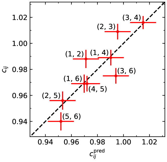
Figure 1: A comparison of NPIPE 12.6 calibration factors $c_{ij}$ measured from the EE spectra and those predicted from triplets of TE spectra. The labels refer to the EE index given in Table 8.

3.4.3 Temperature-to-polarization leakage

In PR3 as well as NPIPE great care was taken to eliminate temperature-to-polarization (TP) leakage due for example to bandpass mismatch or ADCNL. Another source of TP leakage is beam mismatch; since polarization maps are created using pairs of bolometers, any mismatch of the beams of the individual bolometers in a pair will create TP leakage in the map. We calculate a correction for this effect using the off-diagonal terms of the beam matrix $W_{\ell}$ computed using QuickPol, as shown in Eq. 4:

$$\bar{\bar{C}}_{\ell}^{TE} =W_{\ell}^{TETE}\tilde{C}_{\ell}^{TE}+W_{\ell}^{TETT}\tilde{C}_{\ell}^{TT}$$ (4a)

$$\bar{\bar{C}}_{\ell}^{EE} =W_{\ell}^{EEEE}\tilde{C}_{\ell}^{EE}+W_{\ell}^{EETT}\tilde{C}_{\ell}^{TT}.$$ (4b)

Here $\bar{\bar{C}}_{\ell}$ is the beam-convolved spectrum while $\tilde{C}_{\ell}$ is beam-corrected; in practice we use theoretical spectra $C_{\ell}^{TT}$ rather than $\tilde{C}_{\ell}^{TT}$ to estimate the leakage corrections. The QuickPol correction of Eq. 4 is applied for TE but found to be negligible for EE.

To test the effectiveness of the leakage correction, we follow the method laid out in EG21 and organize the uncorrected TE spectra into ‘triplets’. Each triplet consists of three spectra all sharing the same polarization map but using different frequency maps in temperature. We expect TP leakage in the polarization map to correlate identically to the dominant CMB component of each temperature map, hence we look for correlated residuals in these triplets as signatures of TP leakage and compare to the correction factor of Eq. 4. The TE spectra are mask and beam deconvolved, corrected for the polarization efficiencies of Table 8, and dust cleaned with 353 GHz. Residuals are calculated with respect to the mean of all TE spectra rather than to a theoretical model to reduce the impact of cosmic variance.

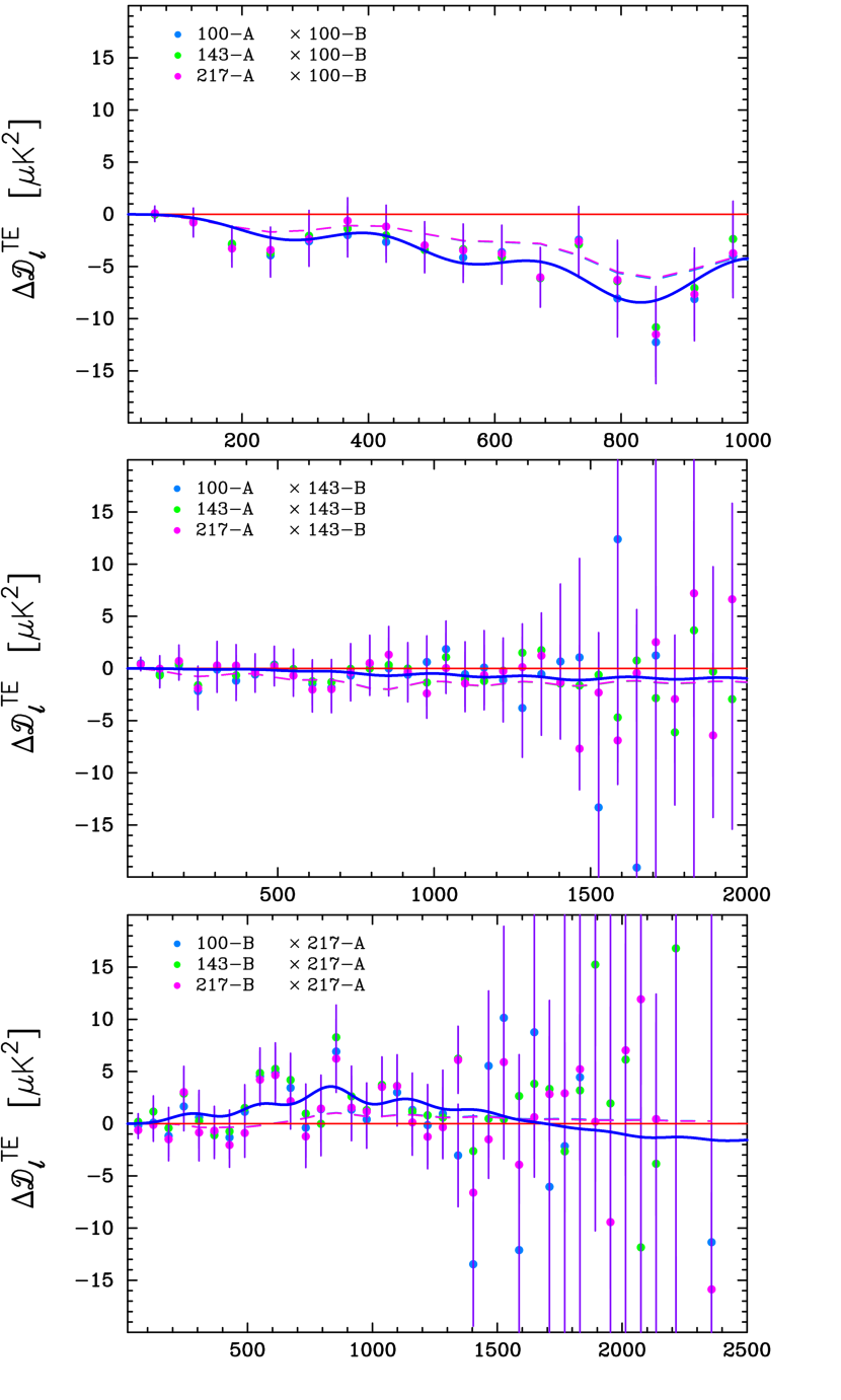
Figure 2: Residuals of NPIPE TE spectra with respect to the mean of all TE spectra. The spectra are mask and beam deconvolved, 353 GHz cleaned, and corrected for effective polarization efficiences. We see a clear correlation between spectra with the same polarization maps, suggesting the residuals are due to TP leakage. Dashed lines show the beam-induced leakage model (from Eq. 4) corrected for in the likelihood. Solid lines are a fit to the residuals.

This test is shown for selected NPIPE spectra in Fig. 2; the solid lines are a fit to the data, while the dotted lines show the leakage correction derived from QuickPol. For 100 GHz, where leakage is most significant, we see excellent agreement between the three spectra using different temperature maps, and between the data and the QuickPol prediction. The same is largely true of the other spectra as well, although there the leakage is quite small. Although the agreement is not perfect, complete neglect of this leakage is found in sec. 6.4 of EG21 to cause up to $1\sigma$ shifts in cosmological parameters; therefore we expect any error from an imperfect leakage model to be significantly less than $1\sigma$. We also note that both the measured and predicted TP leakage is quite different between NPIPE detector sets and the PR3 half-missions presented in EG21, being for example of a similar magnitude but opposite sign in 100 GHz. Since the leakage correction is calculated from QuickPol in the same way in each case, we attribute this difference to the different split of the data in the two analyses.

3.5 Noise Estimation and Covariances

We use analytic covariance matrices as given in the appendix A.2 of EG21. To model the noise in Planck we estimate a noise power spectrum for each map and fit it with an analytic function of the form

$$N_{\ell}=A\left(\frac{100}{\ell}\right)^{\alpha}+B\frac{\left(\ell/1000\right)^{\beta}}{\left(1+\left(\ell/\ell_{c}\right)^{\gamma}\right)^{\delta}}.$$ (5)

Here $A$, $\alpha$, $B$, $\beta$, $\ell_{c}$, $\gamma$, and $\delta$ are free parameters. Weight functions $\psi_{\ell}=N_{\ell}/N_{\ell}^{\mathrm{white}}$ are computed for each $T$, $Q$, $U$ component, and the pixel noise estimates $(\sigma^{X})^{2}_{i}$ in the original formulae for the covariances are replaced by $\sqrt{\psi^{X}_{\ell}\psi^{X}_{\ell^{\prime}}}(\sigma^{X})^{2}_{i}$.

Accurate modeling of the noise is especially important for the noise-dominated polarization spectra and has been a persistent challenge. Traditionally we have estimated noise spectra using differences of data splits. The Plik likelihood in PPL18 uses half-ring difference (HRD) maps for this purpose – half-ring maps are made using the first or second halves of each pointing period and their difference gives an estimate of the noise. The PR3 half-ring maps are known to be correlated due to the glitch processing, so the HRD spectra are an underestimate of the true noise level. In PPL18 this effect was corrected for with an empirical bias correction; EG21 chose instead to use odd-even ring differences (OED), calculated similarly to HRDs but using odd and even rings. There is evidence that these maps overestimate the noise, particularly for $100\times 100$ GHz and at large scales, but in this paper we continue to use them for PR3.

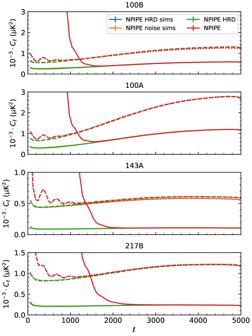
Figure 3: NPIPE noise spectra before mask and beam deconvolution. Solid, dashed, and dotted lines show the auto-spectra of T, Q, and U maps respectively. For each frequency and split we show the auto-spectrum, half-ring difference (HRD) spectrum, and the simulated version of each. For the simulations we show the mean of 100 simulations. 143B and 217A are qualitatively similar to 143A/217B and are omitted.

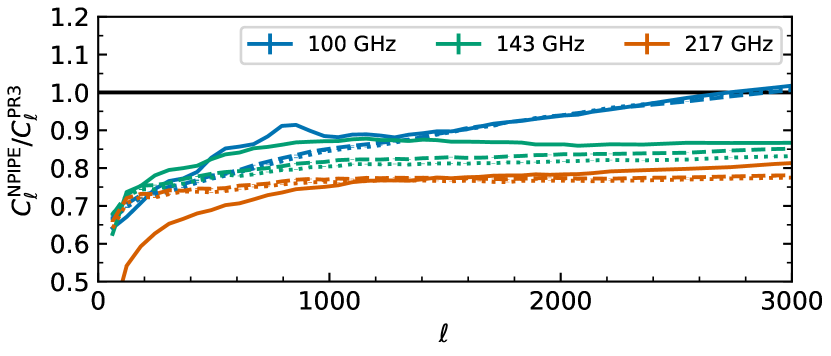
Figure 4: NPIPE undeconvolved full-mission simulated noise spectra divided by their PR3 counterparts. Solid, dashed, and dotted lines show auto-spectra of T, Q, and U maps respectively.

In Fig. 3 we present noise power spectra for NPIPE, comparing noise estimates derived from simulations to auto-spectra of the detector-set maps and to HRDs. From all panels of Fig. 3 we see no evidence of underestimation of the noise by NPIPE HRDs at a level that would affect our analysis. NP20 attributes this reduction in half-ring correlations to the changes in the glitch processing. We observe excellent agreement between the NPIPE simulations, half-ring differences and auto-spectra at high multipoles. Below $\ell$ of 2000 however the half-ring difference spectra can be below the simulations by a few percent in polarization and up to 5% in temperature, especially at 100 GHz. NP20 also introduces a small-scale ‘noise alignment’ correction to the simulated noise spectra in order to match to $\mathrm{A}-\mathrm{B}$ difference spectra. This further boosts the simulated noise power by 1-2% in both temperature and polarization. These differences are of similar order to the accuracy of the fitting function Eq. 5, which is able to match the spectra to the 1-2% level in polarization and 5% in temperature. The current version of the NPIPE likelihood also neglects to weight the half-ring difference map with per-pixel variances $w_{i}=\sigma_{1}\sigma_{2}/(\sigma^{2}_{1}+\sigma^{2}_{2})$ (see eq. 5.3 of EG21), instead using a constant weighting of 0.5. This leads to a 10% overestimate of the QQ noise for 100B and 143B and smaller (1-2%) errors in polarization for other spectra. The effect on parameters should be small, but will be corrected in future work.

In Fig. 4 we see that NPIPE has somewhat lower noise levels than the PR3 maps, potential overestimation from odd-even maps aside. This is expected to be due primarily to the addition of repointing data and the use of short baselines in destriping, and results in a 10-30% noise reduction at the scales we use, dependent on frequency and multipole.

3.6 Correlated Noise

We use cross-spectra of the NPIPE half-ring difference maps to check for correlated noise, with examples from $143\times 217$ shown in Fig. 5 and others in Fig. 20. These spectra are consistent with zero, indicating there is negligible correlated noise; notably this is also true for $\mathrm{A}\times\mathrm{A}$ and $\mathrm{B}\times\mathrm{B}$ spectra. In particular we find that unlike for the PR3 detector sets the $143\times 143$ and $217\times 217$ TT spectra show no evidence of correlated noise. The most obvious deviations from zero are at high-$\ell$ in the $143\mathrm{B}\times 217\mathrm{B}$ EE spectrum, where the noise is nevertheless very high. Therefore we hope to add all AA and BB spectra in TE and EE to a future version of the likelihood as the addition of 6 spectra – AA and BB for each of $100\times 143$, $100\times 217$, and $143\times 217$ – would significantly improve the constraining power of EE. TE would improve by a smaller amount as each new spectrum is equivalent to one already in the likelihood up to A-B exchange of the already signal-dominated temperature map.

Figure 5: NPIPE half-ring difference cross-spectra for $143\times 217$ GHz. Error bars show the standard deviation $\sigma/\sqrt{\Delta\ell}$ within each bandpower of bin-width $\Delta\ell$. Vertical lines indicate the $\ell$-range used in the likelihood.

3.7 New likelihoods and nomenclature

Before discussing the spectra and parameter constraints in more detail we pause to introduce the nomenclature surrounding our likelihoods. As discussed previously our new likelihoods build on CamSpec12.5HMcl, presented in EG21. The covariance matrices of 12.5HMcl included contributions from foregrounds despite being a foreground-cleaned likelihood; this led to some overestimation of the error bars at high multipoles. This had negligible effect on cosmology but affected $\chi^{2}$ values in TT and has been corrected in the new 12.6HMcl, which in this paper we will call PR3_12.6. Using NPIPE A and B maps in place of PR3 half-mission maps and half-ring instead of odd-even noise estimates we have an analogous NPIPE likelihood, PR4_12.6.

4 Spectra and Consistency Checks

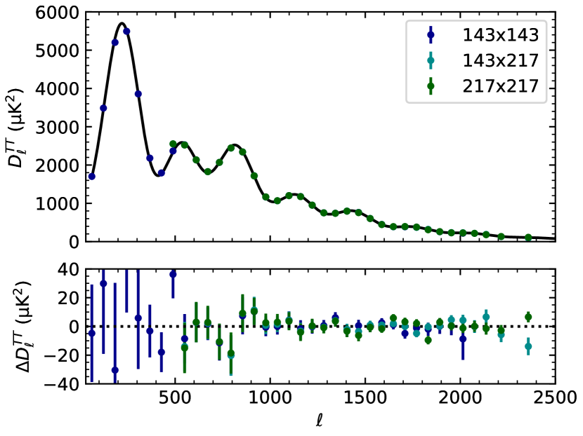
Figure 6: NPIPE 12.6 TT power spectra with best-fit foregrounds removed. Residuals are shown with respect to the TTTEEE best-fit theory.

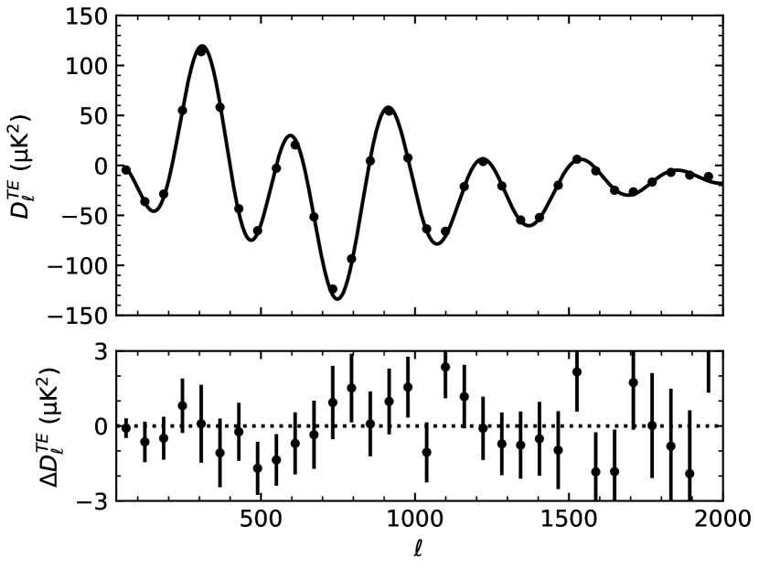
Figure 7: NPIPE 12.6 TE power spectrum and residual with respect to the TTTEEE best-fit theory.

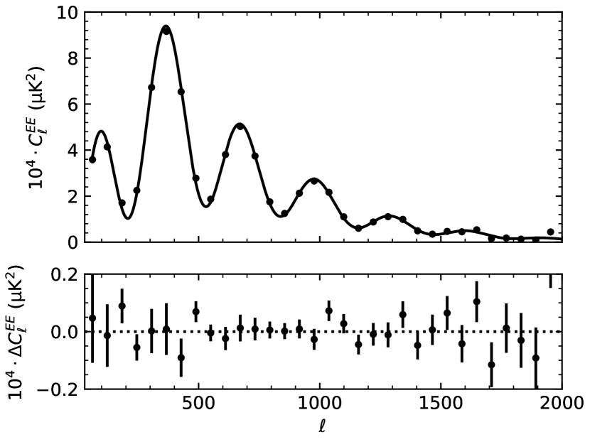
Figure 8: NPIPE 12.6 EE power spectrum and residual with respect to the TTTEEE best-fit theory.

Figure 9: TT power spectrum residuals with respect to the PR4_12.6 TT best-fit. Best-fit foreground residuals have been subtracted from the data points, while calibrations have been applied to the theories. The best-fit theory to PR3_12.6 TT is shown as a solid red line. Points are slightly offset for visual clarity.

As in CamSpec 12.5HMcl we use co-added spectra at $143\times 143$, $143\times 217$, and $217\times 217$ GHz in TT, while co-adding all $\mathrm{A}\times\mathrm{B}$ cross-spectra of 100, 143, and 217 GHz in TE and EE. The multipole ranges used are given in Table 9. Co-added NPIPE 12.6 power spectra are shown in Figs. 6 (TT), 7 (TE) and 8 (EE), with residuals to the $\mathrm{\Lambda CDM}$ best-fit to TTTEEE (discussed in Sec. 5). Note that we plot binned data here for clarity, but the actual likelihood is unbinned.

Visually the $\mathrm{\Lambda CDM}{}$ best-fit shown in Figs. 6-8 appears to match the spectra well; to more quantitatively check the agreement of the data and the model for PR4_12.6 we calculate $\chi^{2}$ values with respect to the TTTEEE best-fit model, shown in Table 1. For each of the individual TT spectra as well as co-added TT, TE and EE we find acceptable values for $\chi^{2}$. However, the $\chi^{2}$ values for total TT and TTTEEE are somewhat large, being over $4\sigma$ high. The source of these high $\chi^{2}$ is primarily at $500\lesssim\ell\lesssim 1000$, and to a lesser extent $\ell<500$. We see the same effect in PR3_12.6, and it was also reported in Planck Collaboration XV (2014). The effect is not unexpected as when all three temperature spectra are present and particularly when as now computed on the same galactic mask, the likelihood may respond to the ‘cosmic variance free’ combination $C_{\ell}^{143\times 143}+C_{\ell}^{217\times 217}-2C_{\ell}^{143\times 217}$ rendering the $\chi^{2}$ particularly sensitive to the accuracy of the noise modeling in these cases as the usually dominant cosmic variance is canceled. Comparing this combination to the expected null spectrum in the multipole range 500-2000 we find a $\chi^{2}$ high by $3.5\sigma$, supporting this interpretation. If we subtract off a version of this spectrum smoothed on a scale of $\Delta\ell=61$ we still find that $\chi^{2}$ is high by $3.1\sigma$. This suggests we are seeing the effects of slightly high scatter throughout the $\ell$-range rather than a smooth trend that could be fit by an improved foreground model or a different cosmology.

At low multipoles (30-500) where we use only $143\times 143$ the $\chi^{2}$ is $2.7\sigma$ higher than expected, but as there is only one spectrum this cannot be explained with the above argument. One possible explanation is the effect of excess variance introduced by the point-source masks that is not captured in the analytical covariance matrices. This effect is explained in depth in appendix C of Planck Collaboration XI (2016). A deviation of up to 10% in the variance is found with the masks used there; from that we estimate that this effect could account for up to about $1\sigma$ of the high variance we see at $\ell<500$. For this region the improvement in $\chi^{2}$ is again marginal when a smoothed spectrum is subtracted, suggesting that relatively smooth cosmologies should not respond to this feature of the likelihood.

PR4_12.6	$\ell$ range	$N_{D}$	$\hat{\chi}^{2}$	$(\hat{\chi}^{2}-1)/\sqrt{2/N_{D}}$
TT 143x143	30 – 2000	1971	1.021	0.67
TT 143x217	500 – 2500	2001	0.985	-0.47
TT 217x217	500 – 2500	2001	1.002	0.05
TT Coadded	30 – 2500	2471	1.025	0.87
TT All	30 – 2500	5973	1.074	4.07
TE	30 – 2000	1971	1.055	1.73
EE	30 – 2000	1971	1.026	0.82
TEEE	30 – 2000	3942	1.046	2.02
TTTEEE	30 – 2500	9915	1.063	4.46

Table 1: $\chi^{2}$ of the different components of the PR4_12.6 likelihood with respect to the TTTEEE best-fit model. $N_{D}$ is the size of the data vector. $\hat{\chi}^{2}=\chi^{2}/N_{D}$ is the reduced $\chi^{2}$. The last column gives the number of standard deviations of $\hat{\chi}^{2}$ from unity.

To further investigate the internal consistency of the NPIPE spectra, we can check how well the best $\mathrm{\Lambda CDM}$ fit to TT alone fits the TE and EE data. From Table 2 we find reduced chi-squareds $\hat{\chi}^{2}_{TE}=1.055$ and $\hat{\chi}^{2}_{EE}=1.026$ using the NPIPE TT best-fit solution. These values are $1.75\sigma$ and $0.83\sigma$ greater than 1 respectively, indicating that the TE and EE data are in acceptable agreement with the prediction of the TT model. We further compare these numbers to the best-fits to the TE and EE data to understand how close the TT model is to the actual minima of the polarization likelihoods. If we assume the TT model represents the truth, then due to over-fitting we expect the $\chi^{2}$ of the TE and EE minima to improve over the ‘true’ (TT) model by a draw from a chi-squared distribution with $N_{\mathrm{DOF}}$ equal to the number of free parameters (see e.g. the appendix of Gratton & Challinor (2020)). For TT-TE we find $\Delta\chi^{2}=2.4$, and for TT-EE $\Delta\chi^{2}=8.2$, roughly in line with the $\Delta\chi^{2}$ we expect for a 7-parameter model (6 $\mathrm{\Lambda CDM}$ parameters and one free calibration) and therefore giving us confidence that the NPIPE polarization and temperature spectra are consistent.

Satisfied that our NPIPE spectra are internally consistent, we compare them directly to the PR3_12.6 spectra in Figs. 9, 10, and 11. Beginning with temperature in Fig. 9, we find the co-added NPIPE TT spectrum to be up to 0.3% low relative to PR3 at $200\lesssim\ell\lesssim 1600$. This is reflected in very small cosmological parameter shifts in TT (see Table 10). In TE (Fig. 10) we see good agreement between the spectra apart from a few exceptional points, and find similar $\mathrm{\Lambda CDM}$ best-fits. The NPIPE residuals are slightly smaller, especially at $\ell>1000$, but with a higher $\chi^{2}$ due to the smaller error bars. There is somewhat more difference between the EE spectra (Fig. 11), with more large-scale power and a slight ‘wavy’ residual that leads to a preference for lower $\theta_{*}$ in NPIPE as will be seen in Fig. 12 and Sec. 5.

To further quantify the level of agreement between the spectra we compare the PR4_12.6 $\mathrm{\Lambda CDM}$ best-fit cosmology to the PR3_12.6 data and vice-versa in Table 3. In doing so we leave the nuisance parameters in the likelihood free, as they are not necessarily expected to be the same for each likelihood. We find $\Delta\chi^{2}=2.5$ between the PR3 and PR4 TTTEEE cosmologies for the PR4 data and $\Delta\chi^{2}=1.4$ for the PR3 data, indicating similar best-fit cosmologies compatible with both datasets; the agreement is similarly good for TT and TE individually. For EE we have $\Delta\chi^{2}=8.8$ with PR4 data and $\Delta\chi^{2}=6.6$ for PR3. As with the visual comparison of Fig. 11, this again indicates some difference between PR3 and PR4 in EE.

$\chi^{2}(\Delta\sigma)$
Data	TT Theory	TE Theory	EE Theory
TE	2080.7 (1.75)	2078.3 (1.71)	2119.1 (2.36)
EE	2023.2 (0.83)	2027.7 (0.90)	2015.0 (0.70)
TEEE	4123.5 (2.04)	4124.9 (2.06)	4161.4 (2.47)

Table 2: Chi-squared values for NPIPE polarization data. The rows give the chi-squared $\chi^{2}$ and the number of standard deviations from unity $\Delta\sigma=(\chi^{2}/N_{D}-1)/\sqrt{2/N_{D}}$ for the TE, EE, and combined TEEE datasets when compared to $\mathrm{\Lambda CDM}$ best-fit models to the TT, TE, and EE data (columns).

$\chi^{2}(\Delta\sigma)$	$\mathrm{NP_{d}-NP_{th}}$	$\mathrm{NP_{d}-PR3_{th}}$	$\mathrm{PR3_{d}-NP_{th}}$	$\mathrm{PR3_{d}-PR3_{th}}$
TT	6417.4 (4.066)	6417.8 (4.070)	6335.0 (3.312)	6334.9 (3.311)
TE	2078.3 (1.709)	2078.8 (1.717)	1965.0 (-0.096)	1964.4 (-0.105)
EE	2015.1 (0.702)	2023.9 (0.843)	1811.9 (-2.534)	1805.3 (-2.637)
TTTEEE	10543.1 (4.460)	10545.5 (4.477)	10116.1 (1.428)	10114.7 (1.418)

Table 3: $\chi^{2}$ comparisons between PR4_12.6 (NP) and PR3_12.6. Each row gives the spectrum used for both the data and the best-fit cosmology. The first column uses NPIPE for both data and theory, the second compares NPIPE data to the best-fit theory from PR3, and so forth. Note that only cosmological parameters are kept fixed in the theory, while nuisance parameters are left free.

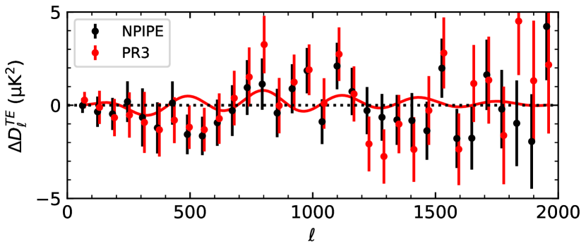
Figure 10: TE power spectrum residuals with respect to the PR4_12.6 TE best-fit. The best-fit theory to PR3_12.6 TE is shown as a solid red line.

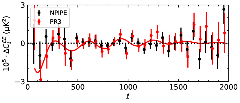
Figure 11: EE power spectrum residuals with respect to the PR4_12.6 EE best-fit. The best-fit theory to PR3_12.6 EE is shown as a solid red line.

5 Base $\Lambda$CDM Results

In this section we describe our constraints on cosmological parameters in the base $\mathrm{\Lambda CDM}$ model using the NPIPE versions of the CamSpec likelihood. We use the standard set of six cosmological parameters for $\mathrm{\Lambda CDM}$ given in Table 4 with their priors. In addition to these cosmological parameters we have nuisance parameters $A^{\rm power}_{\nu}$ and $\gamma^{\rm power}_{\nu}$ for each TT spectrum, representing the amplitudes and spectral indices of power-law fits to remaining foreground residuals:

$$D_{\ell}^{\rm power}=A^{\rm power}\left(\frac{\ell}{1500}\right)^{\gamma^{\rm power}}.$$ (6)

These nuisance parameters are necessary to capture excesses from CIB and point sources in temperature that are not removed by 545 GHz cleaning. Any small foreground residuals remaining after power-law subtraction are ignored in the spectra and covariances. There are also three calibration parameters by which the theory is divided in the likelihood: the overall calibration $A_{\mathrm{Planck}}^{2}$ and individual polarization calibrations $C_{\mathrm{TE}}$ and $C_{\mathrm{EE}}$. Because all of our likelihoods are limited to $\ell\geq 30$ we supplement with low-$\ell$ ($2\leq\ell\leq 29$) likelihoods from PR3; for all temperature likelihoods we include the Commander TT likelihood (Planck Collaboration IV, 2020) and for polarization we add the SimAll EE likelihood (Planck Collaboration III, 2020).

	Prior limits
$\log(10^{10}A_{\mathrm{s}})$	1.61-3.91
$100\theta_{\mathrm{MC}}$	0.5-10
$n_{\mathrm{s}}$	0.8-1.2
$\Omega_{\mathrm{b}}h^{2}$	0.005-1
$\Omega_{\mathrm{c}}h^{2}$	0.001-0.99
$\tau_{\mathrm{reio}}$	0.01-0.8
$A_{\mathrm{Planck}}$	$\mu=1$; $\sigma=0.0025$
$c_{\mathrm{TE}}$	$\mu=1$; $\sigma=0.01$
$c_{\mathrm{EE}}$	$\mu=1$; $\sigma=0.01$
$A^{\rm power}_{143}$	0-50
$A^{\rm power}_{217}$	0-50
$A^{\rm power}_{\mathrm{143x217}}$	0-50
$\gamma^{\rm power}_{143}$	0-5
$\gamma^{\rm power}_{217}$	0-5
$\gamma^{\rm power}_{\mathrm{143x217}}$	0-5

Table 4: Prior ranges on sampled parameters in both PR3_12.6 and PR4_12.6. Gaussian priors with mean $\mu$ and standard deviation $\sigma$ are used for the calibrations, all other priors are flat. The TE and EE calibration parameters are not used in temperature-only likelihoods, and the foreground nuisance parameters $A^{\rm power}_{\nu}$ and $\gamma^{\rm power}_{\nu}$ are not used in polarization-only likelihoods.

In Fig. 12 we compare parameter constraints from NPIPE TT, TE and EE, again assessing agreement between the components. We find that the TT and TE constraints are highly consistent, and have similar constraining power; the EE constraints are broader but serve as a useful consistency check for Planck. Treating TT and EE as independent, we approximately quantify the consistency between their parameter constraints as follows. From our MCMC chains we compute a data vector of mean posterior values $P$ and covariances $C$ for our six sampled $\mathrm{\Lambda CDM}$ parameters. In this 6-dimensional space we calculate $\Delta_{P}=P_{\mathrm{TT}}-P_{\mathrm{EE}}$ and $C_{\Delta}=C_{\mathrm{TT}}+C_{\mathrm{EE}}$, finding $\chi^{2}=\Delta_{P}^{\mathrm{T}}C_{\Delta}^{-1}\Delta_{P}=7.31$, indicating agreement within 0.5$\sigma$. Indeed, EE is very consistent for all parameters except the acoustic scale parameter $\theta_{*}$, for which EE prefers a somewhat lower value (2.8$\sigma$ lower than TT). This is reminiscent of the similar preference in PR3 EE for high $n_{s}$ relative to TT and TE which has disappeared in PR4_12.6. The $\theta_{*}$ tension is also slightly worse for extended models: for $\mathrm{\Lambda CDM}+A_{L}$ we have a $3.3\sigma$ difference, and for $\mathrm{\Lambda CDM}+\Omega_{K}$ $3.2\sigma$, due primarily to an increase in $\theta_{*}$ preferred by the TT spectrum in these models. Referring back to Fig. 12 however (see also Fig. 16), note that there is still substantial overlap of the $\theta_{*}$ contours; this is also true in the extended models. Given the consistency of NPIPE TT and TE on $\theta_{*}$, which also agree very well with the values from PR3_12.6, we do not regard this shift as evidence for lower $\theta_{*}$. Rather it is more likely due to parameter degeneracies coupling to residual systematics in EE (the spectrum most likely to be affected by systematics), or perhaps a statistical fluctuation.

Moving on to the full TTTEEE likelihood, we present a comparison of $\mathrm{\Lambda CDM}$ parameter constraints from PR4_12.6 and PR3_12.6 in Table 5. Two-dimensional marginalized constraints, alongside those from the 2018 Plik likelihood and HiLLiPoP (see Sec. 7), are given in Fig. 13. We find consistency at the sigma level among all four likelihoods, for all cosmological parameters. Given the small weight carried by EE in a TTTEEE likelihood, note that any issues with EE or differences in their handling will have little impact on the overall cosmological constraints. The NPIPE likelihood contours are smaller than for PR3_12.6, and significantly more constraining than Plik. The widths of the 1-dimensional 68% constraints, as given in Table 5, shrink between 7% and 14% (14-21%) compared to PR3_12.6 (Plik) TTTEEE for $\Omega_{\mathrm{b}}h^{2}$, $\Omega_{\mathrm{c}}h^{2}$, $\theta_{*}$, $n_{\mathrm{s}}$, and $H_{0}$. Such decreases are consistent with the lower noise levels discussed in Sec. 3.5.

	PR4_12.6	PR4_12.6	PR3_12.6
	TT	TTTEEE	TTTEEE
$\Omega_{\mathrm{b}}h^{2}$	$0.02209\pm 0.00019$	$0.02218\pm 0.00013$	$0.02225\pm 0.00014$
$\Omega_{\mathrm{c}}h^{2}$	$0.1196\pm 0.0018$	$0.1197\pm 0.0011$	$0.1197\pm 0.0012$
$100\,\theta_{\mathrm{MC}}$	$1.04083\pm 0.00039$	$1.04075\pm 0.00024$	$1.04102\pm 0.00027$
$\tau$	$0.0515\pm 0.0073$	$0.0517\pm 0.0072$	$0.0533\pm 0.0074$
$\ln(10^{10}A_{\mathrm{s}})$	$3.034\pm 0.015$	$3.035\pm 0.015$	$3.041\pm 0.015$
$n_{\mathrm{s}}$	$0.9626\pm 0.0052$	$0.9635\pm 0.0039$	$0.9667\pm 0.0042$
$H_{0}$	$67.26\pm 0.79$	$67.26\pm 0.49$	$67.40\pm 0.54$
$100\,\theta_{*}$	$1.04107\pm 0.00038$	$1.04098\pm 0.00024$	$1.04123\pm 0.00027$
$\Omega_{\Lambda}$	$0.685\pm 0.011$	$0.6849\pm 0.0068$	$0.6859\pm 0.0076$
$\Omega_{\mathrm{m}}$	$0.315\pm 0.011$	$0.3150\pm 0.0068$	$0.3140\pm 0.0076$
$\Omega_{\mathrm{m}}h^{2}$	$0.1423\pm 0.0017$	$0.1425\pm 0.0011$	$0.1426\pm 0.0012$
$\sigma_{8}$	$0.8060\pm 0.0082$	$0.8067\pm 0.0067$	$0.8098\pm 0.0070$
$\sigma_{8}\Omega_{\mathrm{m}}^{0.5}$	$0.452\pm 0.011$	$0.4528\pm 0.0072$	$0.4538\pm 0.0079$
$\sigma_{8}\Omega_{\mathrm{m}}^{0.25}$	$0.604\pm 0.010$	$0.6043\pm 0.0070$	$0.6062\pm 0.0075$
$z_{\mathrm{re}}$	$7.42\pm 0.76$	$7.43^{+0.75}_{-0.68}$	$7.58\pm 0.75$
$10^{9}A_{\mathrm{s}}$	$2.079\pm 0.032$	$2.081\pm 0.031$	$2.092\pm 0.032$
$10^{9}A_{\mathrm{s}}e^{-2\tau}$	$1.875\pm 0.013$	$1.877\pm 0.011$	$1.880\pm 0.011$
$\mathrm{Age}/\mathrm{Gyr}$	$13.826\pm 0.031$	$13.820\pm 0.020$	$13.806\pm 0.022$
$r_{\mathrm{drag}}$	$147.52\pm 0.43$	$147.40\pm 0.25$	$147.31\pm 0.28$
$A_{\mathrm{Planck}}$	$1.0004\pm 0.0024$	$1.0004\pm 0.0024$	$1.0005\pm 0.0024$
$c_{\mathrm{TE}}$	-	$0.9975\pm 0.0036$	$1.0005\pm 0.0041$
$c_{\mathrm{EE}}$	-	$0.9975\pm 0.0037$	$1.0013\pm 0.0043$
$A^{\rm power}_{143}$	$19.1^{+2.0}_{-2.8}$	$18.1^{+1.7}_{-2.4}$	$17.2^{+1.9}_{-2.4}$
$A^{\rm power}_{143\times 217}$	$9.8^{+1.9}_{-2.7}$	$8.8^{+1.6}_{-2.3}$	$8.0^{+1.7}_{-2.4}$
$A^{\rm power}_{217}$	$12.9^{+1.9}_{-2.7}$	$11.9^{+1.6}_{-2.3}$	$12.8^{+1.7}_{-2.4}$
$\gamma^{\rm power}_{143}$	$0.97^{+0.23}_{-0.17}$	$1.01^{+0.20}_{-0.17}$	$1.12^{+0.28}_{-0.24}$
$\gamma^{\rm power}_{143\times 217}$	$1.54^{+0.53}_{-0.61}$	$1.72^{+0.54}_{-0.61}$	$1.53^{+0.51}_{-0.74}$
$\gamma^{\rm power}_{217}$	$1.39\pm 0.42$	$1.52\pm 0.41$	$1.40\pm 0.39$

Table 5: PR4_12.6 parameter constraints in $\mathrm{\Lambda CDM}$, with a comparison to PR3_12.6. We report mean values and 68% confidence intervals. Further entries are given in Table 10.

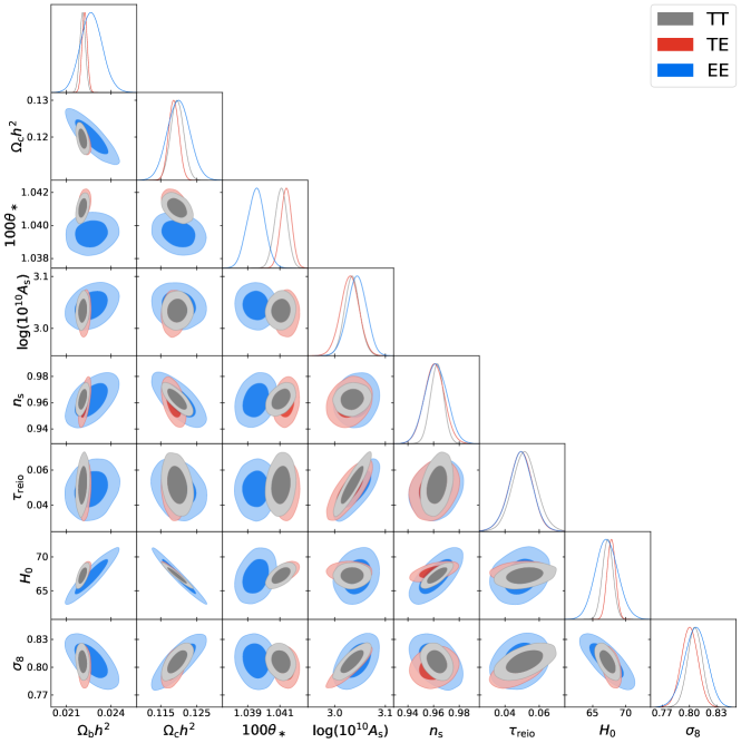
Figure 12: Comparison of 68% and 95% limits on cosmological parameters in $\mathrm{\Lambda CDM}$ from the NPIPE TT, TE, and EE likelihoods.

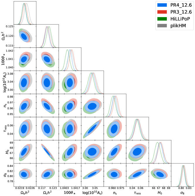
Figure 13: 2D 68% and 95% parameter constraints on cosmological parameters in $\mathrm{\Lambda CDM}$ using the PR4_12.6, PR3_12.6, HiLLiPoP (PR4), and Plik (PR3) TTTEEE likelihoods. Note that the scales are zoomed in relative to Figure 12.

6 Extended Models

We turn now to constraints of single-parameter extensions to the $\mathrm{\Lambda CDM}$ model. In particular we have varied curvature $\Omega_{K}$, the phenomenological $A_{L}$ parameter, the effective number of light species $N_{\mathrm{eff}}$, and the sum of the neutrino masses $m_{\nu}$ one at a time. Marginalized constraints on each of these parameters are presented in Table 6, but we focus our discussion on $\Omega_{K}$ and $A_{L}$.

PR4_12.6	$A_{L}$	$\Omega_{K}$	$N_{\mathrm{eff}}$	$m_{\nu}$
TTTEEE	$1.095\pm 0.056$	$-0.025^{+0.013}_{-0.010}$	$3.00\pm 0.21$	$<0.161$
TT	$1.198\pm 0.084$	$-0.042^{+0.022}_{-0.016}$	$2.98^{+0.28}_{-0.35}$	$<0.278$
TE	$0.96\pm 0.15$	$-0.010^{+0.035}_{-0.015}$	$3.11^{+0.38}_{-0.42}$	$<0.400$
EE	$0.995\pm 0.15$	$-0.012^{+0.034}_{-0.017}$	$4.6\pm 1.3$	$<2.37$
PR3_12.6	$A_{L}$	$\Omega_{K}$	$N_{\mathrm{eff}}$	$m_{\nu}$
TTTEEE	$1.146\pm 0.061$	$-0.035^{+0.016}_{-0.012}$	$2.94^{+0.20}_{-0.23}$	$<0.143$
TT	$1.215\pm 0.089$	$-0.047^{+0.024}_{-0.017}$	$2.89^{+0.28}_{-0.32}$	$<0.248$
TE	$0.96\pm 0.17$	$-0.015^{+0.043}_{-0.015}$	$2.96^{+0.42}_{-0.49}$	$<0.504$
EE	$1.15\pm 0.20$	$-0.053^{+0.063}_{-0.029}$	$2.46^{+0.94}_{-1.7}$	-

Table 6: Mean values and 68% limits for beyond-$\mathrm{\Lambda CDM}$ parameters.

Starting with $\Omega_{K}$ we see a notable difference between NPIPE and PR3 polarization. The TT results hardly change, but in TE and especially EE we find with NPIPE a significant shrinking of the error bars, accompanied by a shift toward $\Omega_{K}=0$, as illustrated in Fig. 14. In particular, the long tails allowing negative $\Omega_{K}$ are significantly reduced. Inspection of the 2D contours (not illustrated) do not suggest any obvious degeneracy between $\Omega_{K}$ and $\theta_{*}$, so this shift in $\Omega_{K}$ appears independent from the low value of $\theta_{*}$ seen above in NPIPE EE. The maximum-likelihood point (best-fit) of PR4_12.6 TTTEEE prefers $\Omega_{K}<0$ at $1.2\sigma$, similar to the $1.6\sigma$ preference in PR3_12.6 but now with a shift of the best-fit from $\Omega_{K}=-0.026$ to $-0.016$ and a 20% decrease in the size of the positive error bar. Similarly, the mean value of the posteriors prefers $\Omega_{K}<0$ at $1.9\sigma$ in PR4_12.6 TTTEEE, down from $2.2\sigma$ in PR3 (see Table 6).

Turning to $A_{L}$, shown in Fig. 15, we see a similar trend to that for $\Omega_{K}$. PR4_12.6 prefers a lower best-fit value of $A_{L}=1.084$ compared to $A_{L}=1.141$ from PR3_12.6, and is now $1.5\sigma$ greater than $A_{L}=1$ rather than $2.3\sigma$. The means (Table 6) find $A_{L}>1$ by $1.7\sigma$ (PR4) and $2.4\sigma$ (PR3). The constraint from EE in particular has shifted to be centered at $A_{L}=1$, while TT and TE show smaller downward shifts with slightly smaller error bars relative to PR3_12.6. Again, there does not appear to be a particular degeneracy between $A_{L}$ and $\theta_{*}$. To better test this we re-run cosmological parameter estimation with $\theta_{*}$ fixed to its PR3_12.6 best-fit value, and find that the NPIPE $A_{L}$ constraints are effectively unchanged. This gives us confidence that the preference for excess smoothing of the power spectra represented by $A_{L}$ really has decreased in the NPIPE maps, independent of other parameter shifts.

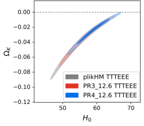
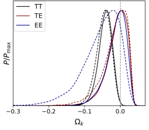
Figure 14: Left: 68% and 95% confidence limits in the $\Omega_{K}-H_{0}$ plane from Plik, PR3_12.6, and PR4_12.6 TTTEEE likelihoods. Right: 1D marginalized densities on $\Omega_{K}$ from TT, TE, and EE. Constraints from NPIPE are shown with solid lines, and PR3_12.6 with dashed lines.

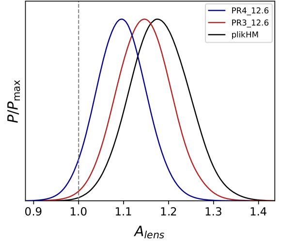
Figure 15: Marginalized constraints on $A_{L}$ from the PR4_12.6, PR3_12.6, and Plik TTTEEE likelihoods.

7 External Comparisons

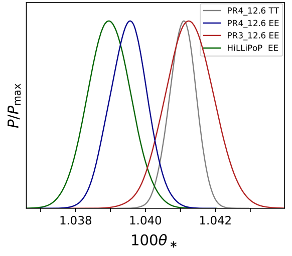
Figure 16: Marginalized constraints on $\theta_{*}$ from PR4_12.6 TT and the PR4_12.6, PR3_12.6, and HiLLiPoP (PR4) EE likelihoods. Both NPIPE EE likelihoods prefer lower values of $\theta_{*}$ relative to PR3 EE or TT.

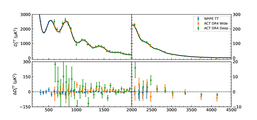
Figure 17: PR4_12.6 and ACT DR4 TT power spectra. NPIPE spectra are foreground-subtracted and binned using the ACT Wide window functions. The lower panels show residuals to the best-fit PR4_12.6 TT power spectrum. At multipoles higher than 2000 we use an expanded scale to better show differences between the spectra.

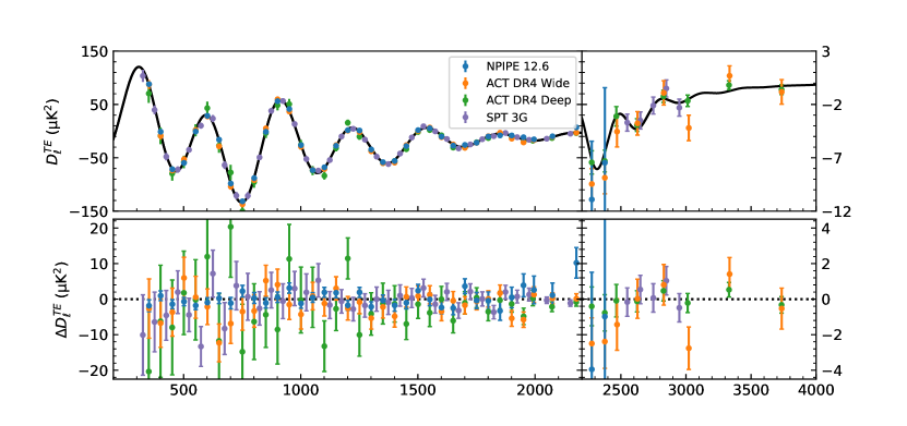
Figure 18: PR4_12.6, ACT DR4, and SPT-3G TE power spectra. The lower panels show residuals to the best-fit PR4_12.6 TE power spectrum, binned using the appropriate window function. NPIPE is binned as ACT Wide. As in Fig. 17 the scale is expanded at high $\ell$.

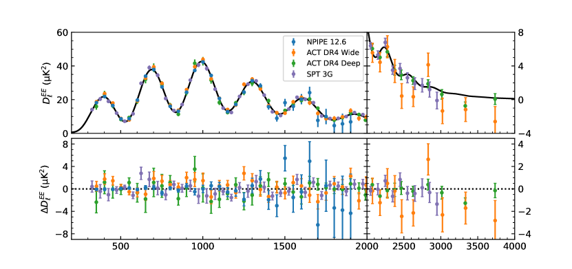
Figure 19: As Fig. 18 for EE.

7.1 HiLLiPoP

A limited analysis of the NPIPE maps using the HiLLiPoP likelihood (Couchot et al., 2017) and focusing on the tensor-to-scalar ratio $r$ has been published in Tristram et al. (2022). HiLLiPoP is also a pseudo-$C_{\ell}$ likelihood and uses NPIPE data products. However the likelihood differs from ours in choice of masks, spectra, and foreground mitigation approach. Instead of cleaning spectra, HiLLiPoP attempts to fit parametric models to uncleaned temperature and polarization spectra, including those using 100 GHz data. Tristram et al. (2022) find high-$\ell$ TT to give essentially identical results to PR3; full high-$\ell$ TE and EE results are not given there due to that paper’s focus on $r$. We use the public HiLLiPoP likelihood with all default prior ranges on nuisance and foreground parameters together with our own priors on cosmological parameters to compare to our CamSpec likelihood. Note that we continue to use Commander and SimAll at low multipoles. These results are shown alongside Plik and our baseline CamSpec and NPIPE constraints in Fig. 13. We find that HiLLiPoP favors an even lower $\theta_{*}$ than PR4_12.6; this is driven by polarization as shown in Fig. 16, while the TT-only constraints (not shown) are similar to those of PR4_12.6. Otherwise the HiLLiPoP constraints do generally agree with our findings at the sigma level.

7.2 ACT DR4 & SPT-3G

We present a simple comparison of our results to the latest ground-based data, ACT DR4 and SPT-3G. More detailed comparisons to plik are presented in the ACT (Choi et al., 2020; Aiola et al., 2020) and SPT (Dutcher et al., 2021) papers, as well as in Handley & Lemos (2021), with a comparison to CamSpec in the appendix of EG21.

For ACT each region, array, and season is independently calibrated to Planck PR3 temperature by cross-correlation. There is no separate polarization calibration; instead there is a free effective polarization efficiency in the likelihood. We compare to co-added CMB-only spectra with foregrounds and temperature-to-polarization leakage corrections marginalized out. SPT also uses Planck PR3 cross-spectra to calibrate temperature of each sub-field before co-addition. They calibrate the final co-added spectra again to both TT and EE, with TE fixed. Foregrounds are not removed from the polarization spectra, but are reported to be negligibly small (Dutcher et al., 2021).

We show power spectra and residuals comparing our NPIPE likelihood PR4_12.6 to ACT DR4 and SPT-3G in Figs. 17, 18, and 19. Table 7 presents $\chi^{2}$ values for the ACT and SPT data using the PR3_12.6 and PR4_12.6 best-fit $\mathrm{\Lambda CDM}$ models. In TT we find generally good agreement between ACT and Planck but see that ACT Wide is consistently high by about 10-20$\mu\mathrm{K}^{2}$ in $D_{\ell}$ from $\ell$ of about 1000 to 1700. Both ACT Deep and Wide are also a bit low relative to Planck at very high multipoles (above 3500). These differences are reflected in somewhat high $\chi^{2}$ values in TT, slightly worse with the NPIPE best-fit than with that of PR3. We interpret this as due to the calibration of ACT DR4 to the PR3 spectra. Indeed, allowing a free calibration parameter decreases the reduced $\chi^{2}$ in TT to 1.30 (PR4) and 1.28 (PR3), confirming that calibration explains most of the difference.

In TE, like TT, the NPIPE spectra are so similar to those from PR3 that previous comparisons to ground-based experiments generally still apply. By eye ACT TE appears to agree well with NPIPE. However we note that Choi et al. (2020) found significant disagreement between PR3 and a subset of ACT TE spectra. There are no obvious features causing this disagreement, and further work is needed to identify its cause. On the SPT side, there is a run of low points at $\ell<700$, while higher multipoles appear to agree well. In EE ACT DR4 Wide is consistently about 5$\mu\mathrm{K}^{2}$ low for $\ell>2500$; otherwise all of the spectra agree well. The TEEE $\chi^{2}$ is very good, being within one sigma for both ACT and SPT. Overall we find, as for PR3, that the three experiments are broadly consistent but a more careful analysis with detailed map-based relative calibration would be necessary for a more quantitative comparison.

Data	PR4_12.6	PR3_12.6	ACT DR4	SPT-3G TEEE
ACT TTTEEE	1.21 (2.43)	1.16 (1.87)	1.08 (0.88)	1.22 (2.51)
ACT TT	1.57 (3.62)	1.48 (3.01)	1.18 (1.15)	1.37 (2.33)
ACT TEEE	1.10 (0.92)	1.09 (0.82)	0.99 (-0.08)	1.19 (1.79)
SPT TEEE	0.98 (-0.34)	0.98 (-0.32)	1.02 (0.29)	0.97 (-0.53)

Table 7: Reduced chi-squared $\hat{\chi}^{2}$ and uncertainties for ACT and SPT data (rows) with $\mathrm{\Lambda CDM}$ best-fits from Planck, ACT, and SPT. The spectra used for each model match the data in all cases except the SPT best-fits, which are always TEEE. Multipole ranges are as in the likelihood for each experiment.

8 Conclusions

In this work we have presented new high-$\ell$ CMB temperature and polarization power spectra and likelihoods using the Planck PR4 ‘NPIPE’ maps. We find excellent consistency between the PR4 and PR3 power spectra, which translates to very good agreement on cosmological parameters as well. The most significant difference is in EE, for which NPIPE prefers a lower value of $\theta_{*}$; however we find that the PR3_12.6 best-fit $\mathrm{\Lambda CDM}$ model is still a good fit to the NPIPE data.

The lower noise of the NPIPE maps leads to tighter parameter constraints, with a ~10% improvement in most $\mathrm{\Lambda CDM}$ parameters in TTTEEE due primarily to improvements in polarization. For $\mathrm{\Lambda CDM}$ extensions we find that, relative to PR3, NPIPE polarization shrinks the error bars on $\Omega_{K}$ and $A_{L}$ from EE by 40% and 25% respectively, and by 15% and 8% in TTTEEE. That these smaller error bars are accompanied by shifts toward the $\mathrm{\Lambda CDM}{}$ values continues the trend observed in EG21 of decreasing the $\Omega_{K}$ and $A_{L}$ tensions as more data is used, as would be expected if these pulls were due to a statistical fluctuation. Overall, we conclude that NPIPE, despite substantial differences in the mapmaking, is completely consistent with PR3 at the power spectrum and parameter levels, offering yet more evidence of the robustness of Planck data and the cosmological results inferred from Planck.

Data Availability

The Planck and NPIPE data products underlying the likelihoods presented here are publicly available at the PLA (http://pla.esac.esa.int/pla/) and at NERSC. The PR3_12.6 and PR4_12.6 likelihoods are both publicly available as internal likelihoods to Cobaya (https://github.com/CobayaSampler/cobaya), named planck_2018_highl_CamSpec2021 (PR3) and planck_NPIPE_highl_CamSpec (PR4).

Appendix A Supplementary tables and figures

This appendix contains the following supplementary information: polarization spectrum calibration factors (Table 8), description of the multipole ranges used in the CamSpec likelihoods (Table 9), half-ring difference cross-spectra for NPIPE (Fig. 20), and $\mathrm{\Lambda CDM}$ parameter constraints for PR4_12.6 and PR3_12.6 TT, TE, and EE likelihoods (Table 10).

Spectrum	TT	$c_{k}$
$143\times 217$		$0.9992\pm 0.0004$
$217\times 217$		$0.9988\pm 0.0005$
Spectrum	EE index	$c_{k}$
$100\mathrm{A}\times 100\mathrm{B}$	(1,2)	$0.988\pm 0.007$
$100\mathrm{A}\times 143\mathrm{B}$	(1,4)	$0.987\pm 0.006$
$100\mathrm{A}\times 217\mathrm{B}$	(1,6)	$0.970\pm 0.007$
$100\mathrm{B}\times 143\mathrm{A}$	(2,3)	$1.008\pm 0.006$
$100\mathrm{B}\times 217\mathrm{A}$	(2,5)	$0.955\pm 0.007$
$143\mathrm{A}\times 143\mathrm{B}$	(3,4)	$1.016\pm 0.005$
$143\mathrm{A}\times 217\mathrm{B}$	(3,6)	$0.975\pm 0.006$
$143\mathrm{B}\times 217\mathrm{A}$	(4,5)	$0.969\pm 0.006$
$217\mathrm{A}\times 217\mathrm{B}$	(5,6)	$0.941\pm 0.007$
Spectrum	TE index	$c_{k}$
$100\mathrm{A}\times 100\mathrm{B}$	(1,2)	$0.985\pm 0.009$
$100\mathrm{A}\times 143\mathrm{B}$	(1,4)	$1.002\pm 0.008$
$100\mathrm{A}\times 217\mathrm{B}$	(1,6)	$0.985\pm 0.009$
$100\mathrm{B}\times 143\mathrm{A}$	(2,3)	$1.010\pm 0.008$
$100\mathrm{B}\times 217\mathrm{A}$	(2,5)	$0.967\pm 0.009$
$143\mathrm{A}\times 143\mathrm{B}$	(3,4)	$0.997\pm 0.008$
$143\mathrm{A}\times 217\mathrm{B}$	(3,6)	$0.980\pm 0.009$
$143\mathrm{B}\times 217\mathrm{A}$	(4,5)	$0.966\pm 0.009$
$217\mathrm{A}\times 217\mathrm{B}$	(5,6)	$0.985\pm 0.009$
$100\mathrm{B}\times 100\mathrm{A}$	(2,1)	$0.980\pm 0.010$
$143\mathrm{B}\times 100\mathrm{A}$	(4,1)	$0.984\pm 0.010$
$217\mathrm{B}\times 100\mathrm{A}$	(6,1)	$0.985\pm 0.010$
$143\mathrm{A}\times 100\mathrm{B}$	(3,2)	$0.983\pm 0.009$
$217\mathrm{A}\times 100\mathrm{B}$	(5,2)	$0.985\pm 0.009$
$143\mathrm{B}\times 143\mathrm{A}$	(4,3)	$1.009\pm 0.008$
$217\mathrm{B}\times 143\mathrm{A}$	(6,3)	$1.015\pm 0.008$
$217\mathrm{A}\times 143\mathrm{B}$	(5,4)	$0.998\pm 0.008$
$217\mathrm{B}\times 217\mathrm{A}$	(6,5)	$0.972\pm 0.009$

Table 8: Calibration factors measured from the NPIPE spectra. Each co-added TT spectrum is multiplied by the given factor upon incorporation into the likelihood. Each TE and EE spectrum is divided (not multiplied) by the relevant factor before coaddition into the single TE and EE spectra of the likelihoods. Indices 1-6 correspond to 100A, 100B, 143A, 143B, 217A, and 217B respectively.

	TT	TE	EE
$100\times 100$	-	$30-1200$	$200-1200$
$100\times 143$	-	$30-1500$	$30-1500$
$100\times 217$	-	$200-1500$	$200-1200$
$143\times 143$	$30-2000$	$30-2000$	$200-2000$
$143\times 217$	$500-2500$	$200-2000$	$300-2000$
$217\times 217$	$500-2500$	$500-2000$	$500-2000$
Total	$30-2500$	$30-2000$	$30-2000$

Table 9: Multipole ranges used in the likelihoods described in this paper.

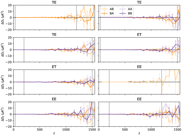
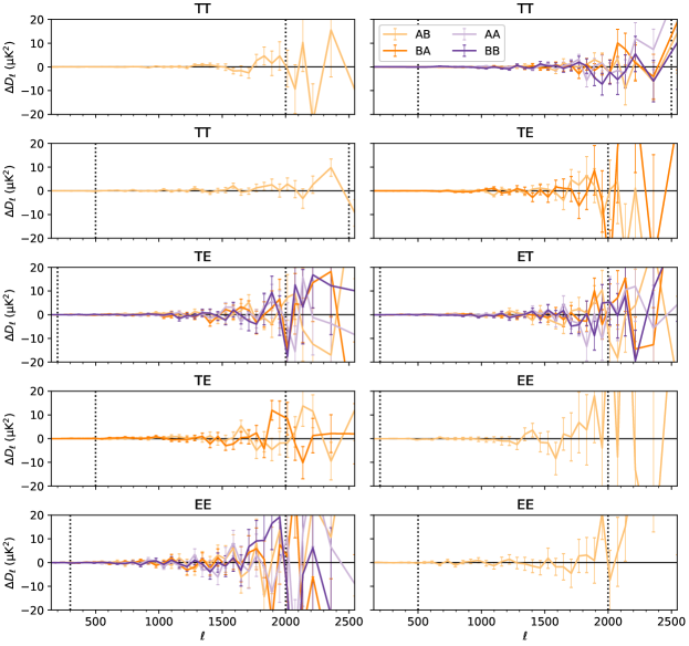
Figure 20: NPIPE half-ring difference cross-spectra. Error bars show the standard deviation $\sigma/\sqrt{\Delta\ell}$ within each bandpower of bin-width $\Delta\ell$.

	PR4_12.6	PR4_12.6	PR4_12.6	PR3_12.6	PR3_12.6	PR3_12.6
	TT	TE	EE	TT	TE	EE
$\Omega_{\mathrm{b}}h^{2}$	$0.02209\pm 0.00019$	$0.02223\pm 0.00017$	$0.02269\pm 0.00073$	$0.02215\pm 0.00020$	$0.02221\pm 0.00019$	$0.02316\pm 0.00093$
$\Omega_{\mathrm{c}}h^{2}$	$0.1196\pm 0.0018$	$0.1186\pm 0.0014$	$0.1200\pm 0.0031$	$0.1193\pm 0.0019$	$0.1191\pm 0.0016$	$0.1161\pm 0.0038$
$100\,\theta_{\mathrm{MC}}$	$1.04083\pm 0.00039$	$1.04117\pm 0.00034$	$1.03934\pm 0.00055$	$1.04073\pm 0.00041$	$1.04142\pm 0.00040$	$1.04114\pm 0.00071$
$\tau$	$0.0515\pm 0.0073$	$0.0490^{+0.0071}_{-0.0064}$	$0.0491\pm 0.0071$	$0.0523\pm 0.0075$	$0.0490\pm 0.0071$	$0.0525\pm 0.0074$
$\ln(10^{10}A_{\mathrm{s}})$	$3.034\pm 0.015$	$3.029\pm 0.019$	$3.044\pm 0.019$	$3.036\pm 0.015$	$3.025\pm 0.019$	$3.040\pm 0.020$
$n_{\mathrm{s}}$	$0.9626\pm 0.0052$	$0.9606\pm 0.0078$	$0.9619\pm 0.0086$	$0.9654\pm 0.0054$	$0.9581\pm 0.0089$	$0.985\pm 0.012$
$H_{0}$	$67.26\pm 0.79$	$67.82\pm 0.62$	$67.1\pm 1.7$	$67.38\pm 0.83$	$67.71\pm 0.72$	$69.5\pm 2.2$
$100\,\theta_{*}$	$1.04107\pm 0.00038$	$1.04139\pm 0.00034$	$1.03951\pm 0.00054$	$1.04096\pm 0.00040$	$1.04164\pm 0.00040$	$1.04126\pm 0.00069$
$\Omega_{\Lambda}$	$0.685\pm 0.011$	$0.6921\pm 0.0085$	$0.681^{+0.023}_{-0.020}$	$0.687\pm 0.011$	$0.6901\pm 0.0098$	$0.709^{+0.026}_{-0.021}$
$\Omega_{\mathrm{m}}$	$0.315\pm 0.011$	$0.3078\pm 0.0085$	$0.319^{+0.020}_{-0.023}$	$0.313\pm 0.011$	$0.3099\pm 0.0098$	$0.291^{+0.021}_{-0.026}$
$\Omega_{\mathrm{m}}h^{2}$	$0.1423\pm 0.0017$	$0.1415\pm 0.0014$	$0.1433\pm 0.0025$	$0.1421\pm 0.0018$	$0.1420\pm 0.0016$	$0.1399\pm 0.0031$
$\sigma_{8}$	$0.8060\pm 0.0082$	$0.8001\pm 0.0093$	$0.807\pm 0.012$	$0.8064\pm 0.0083$	$0.7997\pm 0.0096$	$0.798\pm 0.015$
$\sigma_{8}\Omega_{\mathrm{m}}^{0.5}$	$0.452\pm 0.011$	$0.4438\pm 0.0096$	$0.455\pm 0.021$	$0.451\pm 0.012$	$0.445\pm 0.011$	$0.430^{+0.024}_{-0.026}$
$\sigma_{8}\Omega_{\mathrm{m}}^{0.25}$	$0.604\pm 0.010$	$0.5959\pm 0.0095$	$0.606\pm 0.018$	$0.603\pm 0.011$	$0.597\pm 0.010$	$0.586\pm 0.022$
$z_{\mathrm{re}}$	$7.42\pm 0.76$	$7.12^{+0.78}_{-0.63}$	$7.05^{+0.75}_{-0.63}$	$7.49\pm 0.76$	$7.13^{+0.78}_{-0.65}$	$7.25\pm 0.72$
$10^{9}A_{\mathrm{s}}$	$2.079\pm 0.032$	$2.069\pm 0.038$	$2.099\pm 0.039$	$2.083\pm 0.032$	$2.061\pm 0.038$	$2.092\pm 0.042$
$10^{9}A_{\mathrm{s}}e^{-2\tau}$	$1.875\pm 0.013$	$1.876\pm 0.022$	$1.902\pm 0.024$	$1.876\pm 0.013$	$1.868\pm 0.023$	$1.883\pm 0.027$
$\mathrm{Age}/\mathrm{Gyr}$	$13.826\pm 0.031$	$13.798\pm 0.026$	$13.812\pm 0.091$	$13.822\pm 0.033$	$13.794\pm 0.029$	$13.69\pm 0.12$
$r_{\mathrm{drag}}$	$147.52\pm 0.43$	$147.62\pm 0.36$	$146.76\pm 0.47$	$147.54\pm 0.43$	$147.50\pm 0.40$	$147.28\pm 0.67$
$A_{\mathrm{Planck}}$	$1.0004\pm 0.0024$	$0.99998\pm 0.0025$	$1.0000\pm 0.0024$	$1.0003\pm 0.0024$	$1.0000\pm 0.0025$	$1.0000\pm 0.0024$
$c_{\mathrm{TE}}$	-	$0.9997\pm 0.0092$	-	-	$0.9997\pm 0.0091$	-
$c_{\mathrm{EE}}$	-	-	$1.0000\pm 0.0091$	-	-	$1.0004\pm 0.0091$
$A^{\rm power}_{143}$	$19.1^{+2.0}_{-2.8}$	-	-	$18.4^{+2.2}_{-2.9}$	-	-
$A^{\rm power}_{143\times 217}$	$9.8^{+1.9}_{-2.7}$	-	-	$9.2^{+2.1}_{-2.9}$	-	-
$A^{\rm power}_{217}$	$12.9^{+1.9}_{-2.7}$	-	-	$14.0^{+2.1}_{-2.9}$	-	-
$\gamma^{\rm power}_{143}$	$0.97^{+0.23}_{-0.17}$	-	-	$1.05^{+0.31}_{-0.25}$	-	-
$\gamma^{\rm power}_{143\times 217}$	$1.54^{+0.53}_{-0.61}$	-	-	$1.32^{+0.50}_{-0.72}$	-	-
$\gamma^{\rm power}_{217}$	$1.39\pm 0.42$	-	-	$1.27\pm 0.41$	-	-

Table 10: PR4_12.6 and PR3_12.6 parameter constraints in $\mathrm{\Lambda CDM}$. We report mean values and 68% confidence intervals. TTTEEE is shown in Table 5.

References

- Aiola et al. (2020) Aiola S., et al., 2020, J. Cosmology Astropart. Phys, 2020, 047
- Astropy Collaboration (2013) Astropy Collaboration 2013, A&A, 558, A33
- Astropy Collaboration (2018) Astropy Collaboration 2018, AJ, 156, 123
- Cartis et al. (2018a) Cartis C., Fiala J., Marteau B., Roberts L., 2018a, arXiv e-prints, p. arXiv:1804.00154
- Cartis et al. (2018b) Cartis C., Roberts L., Sheridan-Methven O., 2018b, arXiv e-prints, p. arXiv:1812.11343
- Choi et al. (2020) Choi S. K., et al., 2020, J. Cosmology Astropart. Phys, 2020, 045
- Couchot et al. (2017) Couchot F., Henrot-Versillé S., Perdereau O., Plaszczynski S., Rouillé d’Orfeuil B., Spinelli M., Tristram M., 2017, A&A, 602, A41
- Delouis et al. (2019) Delouis J. M., Pagano L., Mottet S., Puget J. L., Vibert L., 2019, A&A, 629, A38
- Dutcher et al. (2021) Dutcher D., et al., 2021, Phys. Rev. D, 104, 022003
- Efstathiou & Gratton (2021) Efstathiou G., Gratton S., 2021, The Open Journal of Astrophysics, 4, 8
- Górski et al. (2005) Górski K. M., Hivon E., Banday A. J., Wandelt B. D., Hansen F. K., Reinecke M., Bartelmann M., 2005, ApJ, 622, 759
- Gratton & Challinor (2020) Gratton S., Challinor A., 2020, MNRAS, 499, 3410
- Handley & Lemos (2021) Handley W., Lemos P., 2021, Phys. Rev. D, 103, 063529
- Harris et al. (2020) Harris C. R., et al., 2020, Nature, 585, 357
- Hivon et al. (2002) Hivon E., Górski K. M., Netterfield C. B., Crill B. P., Prunet S., Hansen F., 2002, ApJ, 567, 2
- Hivon et al. (2017) Hivon E., Mottet S., Ponthieu N., 2017, A&A, 598, A25
- Howlett et al. (2012) Howlett C., Lewis A., Hall A., Challinor A., 2012, JCAP, 1204, 027
- Hunter (2007) Hunter J. D., 2007, Computing in Science & Engineering, 9, 90
- Keihänen et al. (2004) Keihänen E., Kurki-Suonio H., Poutanen T., Maino D., Burigana C., 2004, A&A, 428, 287
- Keihänen et al. (2005) Keihänen E., Kurki-Suonio H., Poutanen T., 2005, MNRAS, 360, 390
- Keihänen et al. (2010) Keihänen E., Keskitalo R., Kurki-Suonio H., Poutanen T., Sirviö A., 2010, A&A, 510, A57
- Kogut et al. (2003) Kogut A., et al., 2003, ApJS, 148, 161
- Lewis (2013) Lewis A., 2013, Phys. Rev., D87, 103529
- Lewis (2019) Lewis A., 2019, arXiv e-prints, p. arXiv:1910.13970
- Lewis & Bridle (2002) Lewis A., Bridle S., 2002, Phys. Rev., D66, 103511
- Lewis et al. (2000) Lewis A., Challinor A., Lasenby A., 2000, Astrophys. J., 538, 473
- Neal (2005) Neal R. M., 2005, arXiv Mathematics e-prints, p. math/0502099
- Planck Collaboration I (2014) Planck Collaboration I 2014, A&A, 571, A1
- Planck Collaboration XV (2014) Planck Collaboration XV 2014, A&A, 571, A15
- Planck Collaboration I (2016) Planck Collaboration I 2016, A&A, 594, A1
- Planck Collaboration VII (2016) Planck Collaboration VII 2016, A&A, 594, A7
- Planck Collaboration XI (2016) Planck Collaboration XI 2016, A&A, 594, A11
- Planck Collaboration I (2020) Planck Collaboration I 2020, A&A, 641, A1
- Planck Collaboration II (2020) Planck Collaboration II 2020, A&A, 641, A2
- Planck Collaboration III (2020) Planck Collaboration III 2020, A&A, 641, A3
- Planck Collaboration IV (2020) Planck Collaboration IV 2020, A&A, 641, A4
- Planck Collaboration V (2020) Planck Collaboration V 2020, A&A, 641, A5
- Planck Collaboration VI (2020) Planck Collaboration VI 2020, A&A, 641, A6
- Planck Collaboration XLVI (2016) Planck Collaboration XLVI 2016, A&A, 596, A107
- Planck Collaboration LVII (2020) Planck Collaboration LVII 2020, A&A, 643, 42
- Powell (2009) Powell M. J. D., 2009, Technical Report, Department of Applied Mathematics and Theoretical Physics, University of Cambridge
- Torrado & Lewis (2021) Torrado J., Lewis A., 2021, J. Cosmology Astropart. Phys, 2021, 057
- Tristram et al. (2022) Tristram M., et al., 2022, Phys. Rev. D, 105, 083524
- Virtanen et al. (2020) Virtanen P., et al., 2020, Nature Methods, 17, 261
- Zonca et al. (2019) Zonca A., Singer L., Lenz D., Reinecke M., Rosset C., Hivon E., Gorski K., 2019, Journal of Open Source Software, 4, 1298