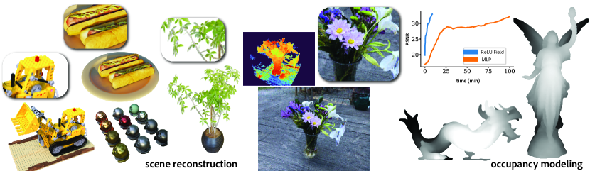
Figure 1. We present a method to represent complex signals such as images or 3D scenes, both volumetric (left) and surface (right), on regularly sampled grid vertices. Our method is able to match the expressiveness of coordinate-based MLPs while retaining reconstruction and rendering speed of voxel grids, without requiring any neural networks or sparse data structures. As a result it converges significantly faster (inset plot).

ReLU Fields: The Little Non-linearity That Could

Abstract.

In many recent works, multi-layer perceptions (MLPs) have been shown to be suitable for modeling complex spatially-varying functions including images and 3D scenes. Although the MLPs are able to represent complex scenes with unprecedented quality and memory footprint, this expressive power of the MLPs, however, comes at the cost of long training and inference times. On the other hand, bilinear/trilinear interpolation on regular grid-based representations can give fast training and inference times, but cannot match the quality of MLPs without requiring significant additional memory. Hence, in this work, we investigate what is the smallest change to grid-based representations that allows for retaining the high fidelity result of MLPs while enabling fast reconstruction and rendering times. We introduce a surprisingly simple change that achieves this task – simply allowing a fixed non-linearity (ReLU) on interpolated grid values. When combined with coarse-to-fine optimization, we show that such an approach becomes competitive with the state-of-the-art. We report results on radiance fields, and occupancy fields, and compare against multiple existing alternatives. Code and data for the paper are available at https://geometry.cs.ucl.ac.uk/projects/2022/relu_fields.

1. Introduction

Coordinate-based Multi-layer Perceptrons have been shown to be capable of representing complex signals with high fidelity and a low memory footprint. Exemplar applications include NeRF [Mildenhall et al., 2020], which encodes lighting-baked volumetric radiance-density field into a single MLP using posed images; LIFF [Chen et al., 2020], which encodes 2D image signal into a single MLP using multi-resolution pixel data. Alternatively, a 3D shape can be encoded as an occupancy field [Mescheder et al., 2019; Chen and Zhang, 2019] or as a signed distance field [Park et al., 2019].

A significant drawback of such approaches is that MLPs are both slow to train and slow to evaluate, especially for applications that require multiple evaluations per signal-sample (e.g., multiple per-pixel evaluations during volume tracing in NeRFs). On the other hand, traditional data structures like $n$-dimensional grids are fast to optimize and evaluate, but require a significant amount of memory to represent high frequency content (see Figure 4). As a result, there has been an explosion of interest in hybrid representations that combine fast-to-evaluate data structures with coordinate-based MLPs, e.g., by encoding latent features in regular [Sun et al., 2021] and adaptive [Liu et al., 2020; Aliev et al., 2020; Martel et al., 2021; Müller et al., 2022] grids and decoding linearly interpolated “neural” features with a small MLP.

In this paper, we revisit regular grid-based models and look for the minimum change needed to make such grids perform on par with “neural” representations. As the key takeaway message, we find that simply using a Rectified Linear Unit (ReLU) non-linearity on top of interpolated grid values, without any additional learned parameters, optimized in a progressive manner already does a surprisingly good job, with minimal added complexity. For example, in Figure 1 we show results in the context of representing volumes (left) and surfaces (right) and on regularly sampled grid vertices for reconstruction, respectively. As additional benefits, these grid based 3D-models are amenable to generative modeling, and to local manipulation.

In summary, we present the following contributions: (i) we propose a minimal extension to grid-based signal representations, which we refer to as ReLU Fields; (ii) we show that this representation is simple, does not require any neural networks, is directly differentiable (and hence easy to optimize), and is fast to optimize and evaluate (i.e. render); and (iii) we empirically validate our claims by showing applications where ReLU Fields plug in naturally: first, image-based 3D scene reconstruction; and second, implicit modeling of 3D geometries.

2. Related Work

Discrete sample based representations

Computer vision and graphics have long experimented with different representations for working with visual data. While working with, images are ubiquitously represented as 2D grids of pixels, while due to the memory requirements; 3D models are often represented (and stored) in a sparse format, e.g., as meshes, or as point clouds. In the context of images, since as early as the sixties [Billingsley, 1966], different ideas have been proposed to make pixels more expressive. One popular option is to store a fixed number (e.g., one) of zero-crossing for explicit edge boundary information [Bala et al., 2003; Tumblin and Choudhury, 2004; Ramanarayanan et al., 2004; Laine and Karras, 2010], by using curves [Parilov and Zorin, 2008], or augmenting pixels/voxels with more than one color [Pavić and Kobbelt, 2010; Agus et al., 2010]. Another idea is to deform the underlying pixel grid by explicitly storing discontinuity information along general curves [Tarini and Cignoni, 2005]. Loviscach [2005] optimized MIP maps, such that the thresholded values match a reference. Similar ideas were also being explored for textures and shadow maps [Sen et al., 2003; Sen, 2004], addressing specific challenges in sampling. ReLU Field grid implicitly stores discontinuity information by varying grid values such that when interpolated and passed through a ReLU it represents a zero crossing per grid cell.

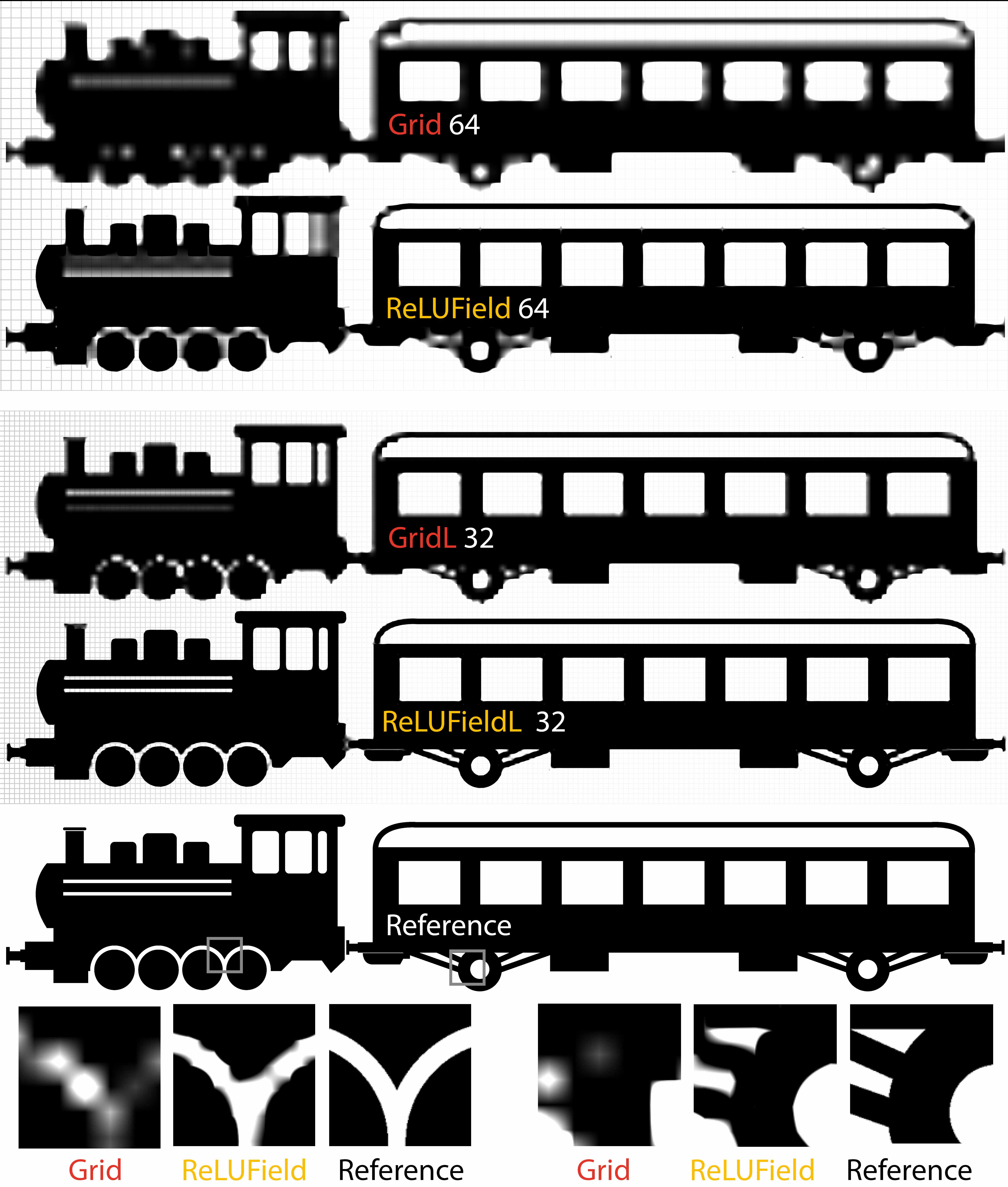
Figure 2. Representing an image with a standard pixel grid bi-linearly interpolated to a larger size (Grid) versus a ReLU Field of the same size (ReLUField). The grid-size of the variants, ReLUField and Grid, is 64x smaller; while of, ReLUFieldL and GridL, is 32x smaller than the source image-resolution along each dimension. Note that the ‘L’ variants have a bigger grid-size and hence less smaller than the GT raster image. Simply adding a ReLU allows for significantly more sharpness and detail to be expressed. Hence, we can say that the humble ReLU is truly the little non-linearity that could.

In the 2D domain, the regular pixel grid format of images has proven to be amenable to machine learning algorithms because CNNs are able to naturally input and output regularly sampled 2D signals as pixel grids. As a result, these architectures can be easily extended to 3D to operate on voxel grids, and therefore can be trained for many learning-based tasks, e.g., using differentiable volume rendering as supervision [Tulsiani et al., 2017; Henzler et al., 2019; Nguyen-Phuoc et al., 2019; Sitzmann et al., 2019]. However, such methods are inefficient with respect to memory and are hence typically restricted to low spatial resolution.

Learned neural representations

Recently, coordinate-based MLPs representing continuous signals have been shown to be able to dramatically increase the representation quality of 3D objects [Groueix et al., 2018] or reconstruction quality of 3D scenes [Mescheder et al., 2019; Mildenhall et al., 2020]. However, such methods incur a high computational cost, as the MLP has to be evaluated, often multiple times, for each output signal location (e.g., pixel) when performing differentiable volume rendering [Mildenhall et al., 2020; Chan et al., 2021b; Schwarz et al., 2020; Niemeyer and Geiger, 2021]. In addition, this representation is not well suited for post-training manipulations as the weights of the MLP have a global effect on the structure of the scene. To fix the slow execution, sometimes grid-like representations are fit post-hoc to a trained Neural Radiance Fields (NeRF) model [Reiser et al., 2021; Hedman et al., 2021; Yu et al., 2021b; Garbin et al., 2021], however such methods are unable to reconstruct scenes from scratch.

As a result, there has been an interest in hybrid methods that store learned features in spatial data structures, and accompany this with an MLP, often much smaller, for decoding the interpolated neural feature signal at continuous locations. Examples of such methods store learned features on regular grids [Sitzmann et al., 2019; Nguyen-Phuoc et al., 2020], sparse voxels [Liu et al., 2020; Martel et al., 2021], point clouds [Aliev et al., 2020], local crops of 3D grids [Jiang et al., 2020], or on intersecting axis-aligned planes (triplane) [Chan et al., 2021a].

Concurrent work

Investigating representations suitable for efficiently representing complex signals is an active area of research. In this section, we discuss three concurrent works: DVGo [Sun et al., 2021], Plenoxels [Yu et al., 2021a] and NGP [Müller et al., 2022].

Reporting a finding similar to ours, DVGo proposes the use of a “post-activated” (i.e., after interpolation) density grid for modelling high-frequency geometries. They model the view-dependent appearance through a learned feature grid which is decoded using an MLP. They in-fact show comprehensive experimental evaluation, on multiple datasets comparing to multiple baselines, for the task of image-based 3D scene reconstruction.

Plenoxels proposes the use of sparse grid structure for modeling the scene with ReLU activation and, similar to our experiments, also uses spherical harmonic coefficients [Yu et al., 2021b] for modeling view-dependent appearance.

NGP [Müller et al., 2022] proposes a hierarchical voxel-hashing scheme to store learned features and using a small MLP decoder for converting them into geometry and appearance. Their reconstruction-times are about significantly lower than the others because of their impressively engineered GPU (low-level cuda) implementation.

We believe that our work differs from these concurrent efforts in that, our motivation is to investigate the minimal change to existing voxel grids that can boost the per-capita signal modelling capacity of the grids when the signals contain sharp c1-discontinuities. And hence as such, we are not focused only on 3D scene reconstruction, and similar to NGP, also consider other applications where grids are the de-facto representation, where ReLU Fields might help. Our method is orthogonal to, and fully compatible with, the sparse data structures proposed in Plenoxels and NGP, and we expect the improvements gained by such approaches to be directly applicable to our work. The power and complexity of other methods, however, comes at the cost of not being able to load the resulting assets into legacy 3D modelling or volume visualization software (backward-compatibility), which is possible for our results, as long as the software can load signed data and apply transfer functions.

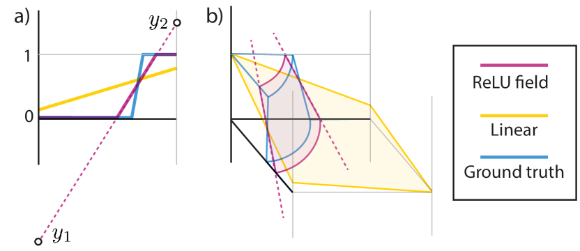
Figure 3. Representing a ground-truth function (blue) in a 1D (a) and 2D (b) grid cell using the linear basis (yellow) and a ReLU Fields (pink). The reference has a c1-discontinuity inside the domain that a linear basis cannot capture. A ReLU Field will pick two values $y_{1}$ and $y_{2}$, such that their interpolation, after clamping will match the sharp c1-discontinuity in the ground-truth (blue) function.

3. Method

It’s Just a Little ReLU

We look for a representation of $n$ -valued signals on an $m$ -dimensional coordinate domain $\mathbb{R}^{m}$. For simplicity, we explain the method for $m=3$. Our representation is strikingly simple. We consider a regular ($m=3$)-dimensional ($r\times r\times r$)-grid $G$ composed of $r$ voxels along each side. Each voxel has a certain size defined by its diagonal norm in the ($m=3$)-dimensional space and holds an $n$ -dimensional vector at each of its ($2^{m=3}=8$) vertices. Importantly, even though they have matching number of dimensions, these values do not have a direct physical interpretation (e.g., color, density, or occupancy), which always have some explicitly-defined range, e.g., $[0,1]$ or $\left[0,+\infty\right)$. Rather, we store unbounded values on the grid; and thus for technical correctness, we call these grids “feature”-grids instead of signal-grids. The features at grid vertices are then interpolated using ($m=3$)-linear interpolation, and followed by a single non-linearity: the ReLU, i.e., function $\mathtt{ReLU}(x)=\max(0,x)$ which maps negative input values to 0 and all other values to themselves. Note that this approach does not have any MLP or other neural-network that interprets the features, instead they are simply clipped before rendering. Intuitively, during optimization, these feature-values at the vertices can go up or down such that the ReLU clipping plane best aligns with the c1-discontinuities within the ground-truth signal. Figure 3 illustrates this concept.

Algorithm 1 Fetching a 2D ReLU field.

1:procedure ReluField2D($G,\mathbf{x}$)

2:     $\mathbf{x}_{\mathrm{g}}$ := Floor($\mathbf{x}$ )

3:     $\mathbf{x}_{\mathrm{f}}$ := Frac($\mathbf{x}$ )

4:     $y_{00}$ := Fetch($G$ , $\mathbf{x}_{\mathrm{g}}$ + (0,0))

5:     $y_{01}$ := Fetch($G$ , $\mathbf{x}_{\mathrm{g}}$ + (0,1))

6:     $y_{10}$ := Fetch($G$ , $\mathbf{x}_{\mathrm{g}}$ + (1,0))

7:     $y_{11}$ := Fetch($G$ , $\mathbf{x}_{\mathrm{g}}$ + (1,1))

8:     y := BiLinear($y_{00}$, $y_{01}$, $y_{10}$, $y_{11}$, $\mathbf{x}_{\mathrm{f}}$)

9:     return relu(y)

10:end procedure

As a didactic example, we fit an image into a 2D ReLU Field grid similar to [Sitzmann et al., 2020], where grid values are stored as floats in the $(-\infty,+\infty)$ range. For any query position, we interpolate the grid values before passing through the ReLU function (see Algorithm 1). Since the image-signal values are expected to be in the $[0,1]$ range, we apply a hard-upper-clip on the interpolated values just after applying the ReLU. We can see in Fig. 2 that ReLU Field allows us to represent sharp edges at a higher fidelity than bilinear interpolation (without the ReLU) at the same resolution grid size. One limitation of this representation is that it can only well represent signals that have sparse c1-discontinuities, such as this flat-shaded images and as we show later, 3D volumetric density. However, other types of signals, such as natural images, do not benefit from using a ReLU Fields representation (see supplementary material).

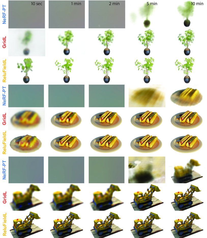
Figure 4. Qualitative comparison between NeRF-PT, GridL and ReLUFieldL. Grid-based versions converge much faster, and we can see significant sharpness improvements of ReLUFieldL over GridL, for example in the leaves of the plant. See also supplementary video.

4. Applications

We now demonstrate two different applications of ReLU Fields; NeRF-like 3D scene-reconstruction (Sec. 4.1), and 3D object reconstruction via occupancy fields (Sec. 4.2).

4.1. Radiance Fields

In this application, we discuss how ReLU Field can be used in place of the coordinate-based MLP in NeRF [Mildenhall et al., 2020]. Input to this approach are a set of images $\mathcal{I}=\{I_{1},\ldots,I_{n}\}$ and corresponding camera poses $\mathcal{C}=\{\mathsf{C}_{1},\ldots,\mathsf{C}_{n}\}$, where each camera pose consists of $\mathsf{C}=\{R,T,0pt,0pt,F\}$; $R$ is the rotation-matrix ($R\in\mathbb{R}^{3\times 3}$), $T$ is the translation-vector ($T\in\mathbb{R}^{3}$), 0pt, 0ptare the scalars representing the height and width respectively, and $F$ denotes the focal length. We assume that the respective poses for the images are known either through hardware calibration or by using structure-from-motion [Schonberger and Frahm, 2016].

We denote the rendering operation to convert the 3D scene representation $\mathcal{S}$ and the camera pose $\mathsf{C}$ into an image as $\mathcal{R}(\mathcal{S},\mathsf{C})$. Thus, given the input set of images $\mathcal{I}$ and their corresponding camera poses $\mathcal{C}$ , the problem is to recover the underlying 3D scene representation $\mathcal{S}$ such that when rendered from any $\mathsf{C}_{i}\in\mathcal{C}$, $\mathcal{S}$ produces rendered image $\hat{I}_{i}$ as close as possible to the input image $I_{i}$, and produces spatio-temporally consistent $\hat{I}_{j}$ for poses $\mathsf{C}_{j}\not\in\mathcal{C}$.

Scene representation

We model the underlying 3D scene representation $\mathcal{S}$ , which is to be recovered, by a ReLU Field. The vertices of the grid store, first, raw pre-$\mathtt{relu}$ density values in $(-\infty,\infty)$ that model geometry, and, second, the second-degree Spherical Harmonics (SH) coefficients [Yu et al., 2021b; Wizadwongsa et al., 2021] that model view-dependent appearance. The $\mathtt{relu}$ is only applied to pre-$\mathtt{relu}$ density, not to appearance.

We directly optimize values at the vertices to minimize the photometric loss between the rendered images $\hat{I}$ and the input images $I$ . The optimized grid $G^{*}$ , corresponding to the recovered 3D scene $\mathcal{S}$ , is obtained as:

(1) $$G^{*}=\operatorname{arg\,min}_{G}\sum_{i=1}^{n}\|I_{i}-\overbrace{\mathcal{R}(G,\mathsf{C}_{i})}^{\text{\footnotesize{$\hat{I}_{i}$}}}\|^{2}_{2}.$$

Implementation details

Similar to NeRF, we use the EA (emission-absorption) raymarching model [Max, 1995; Henzler et al., 2019; Mildenhall et al., 2020] for realizing the rendering function $\mathcal{R}$ . The grid is scaled to a single global AABB (Axis-Aligned-Bounding-Box) that is encompassed by the camera frustums of all the available poses $\mathcal{C}$ , and is initialized with uniform random values. We optimize the vertex values using Adam [Kingma and Ba, 2014] with a learning rate of 0.03, and all other default values, for all examples shown.

We perform the optimization progressively in a coarse-to-fine manner similar to Karras et al. [2018]. Initially, the feature grid is optimized at a resolution where each dimension is reduced by a factor of $2^{4}$. After a fixed number of iterations at each stage $N$, the grid resolution is doubled and the features on the feature-grid $G$ are tri-linearly upsampled to initialize the next stage. This proceeds until the final target resolution is reached.

Table 1. Evaluation results on 3D synthetic scenes. Metrics used are PSNR ($\uparrow$) / LPIPS ($\downarrow$). The column NeRF-TF^∗ quotes PSNR values from prior work [Mildenhall et al., 2020], and as such we do not have a comparable runtime for this method.

Scene	NeRF-TF∗		NeRF-PT		Grid		GridL		ReLUField		ReLUFieldL		RFLong		RFNoPro
	PSNR	LPIPS	PSNR	LPIPS	PSNR	LPIPS	PSNR	LPIPS	PSNR	LPIPS	PSNR	LPIPS	PSNR	LPIPS	PSNR	LPIPS
Chair	33.00	0.04	33.75	0.03	25.53	0.12	27.08	0.11	31.50	0.05	32.39	0.03	31.77	0.05	13.85	0.48
Drums	25.01	0.09	23.82	0.12	19.85	0.20	20.70	0.17	23.13	0.09	25.15	0.06	23.78	0.09	10.74	0.52
Ficus	30.13	0.04	28.96	0.04	22.10	0.13	23.61	0.11	25.89	0.06	27.37	0.04	26.11	0.05	13.21	0.47
Hotdog	36.18	0.12	33.52	0.06	28.53	0.12	29.83	0.10	34.65	0.03	35.72	0.03	34.70	0.03	12.22	0.53
Lego	32.54	0.05	28.36	0.08	23.76	0.17	23.97	0.15	28.83	0.06	30.78	0.03	29.64	0.05	10.63	0.56
Materials	29.62	0.06	29.23	0.04	21.87	0.18	22.74	0.13	27.41	0.06	28.23	0.05	28.23	0.05	8.99	0.55
Mic	32.91	0.02	33.08	0.02	25.87	0.08	25.91	0.08	31.88	0.03	32.62	0.02	31.22	0.03	12.47	0.41
Ship	28.65	0.20	29.22	0.14	23.86	0.25	22.54	0.24	26.86	0.14	28.02	0.12	27.39	0.13	9.92	0.59
Average	31.01	0.07	29.99	0.07	23.92	0.16	24.54	0.14	28.77	0.07	30.04	0.05	29.10	0.06	11.50	0.51
Time (recon)	—		11h:21m:00s		00h:03m:41s		00h:10m:02s		00h:03m:41s		00h:10m:36s		10h:51m:29s		00h:07m:11s
Time (render)	—		16,363.0 ms		9.0 ms		99.1 ms		9.1 ms		99.5 ms		9.1 ms		9.1 ms

Evaluation

We perform experiments on the eight synthetic Blender scenes used by NeRF [Mildenhall et al., 2020], viz. Chair, Drums, Ficus, Hotdog, Lego, Materials, Mic, and Ship and compare our method to prior works, baselines, and ablations. We also show an extension of ReLU Fields to one of their real world captured scenes, named Flowers.

First, we compare to the mlp-based baseline NeRF [Mildenhall et al., 2020]. For the purpose of these experiments though, we use the public nerf-pytorch version [ner, 2021] for comparable training-time comparisons since all our implementations are in PyTorch. For disambiguation, we refer to this PyTorch version as NeRF-PT and the original one as NeRF-TF and report scores for both. Second, we compare to two versions of traditional grids where vertices store scalar density and second-degree SH approximations of the appearance, namely Grid (i.e., $128^{3}$ grid) and GridL (i.e., $256^{3}$ grid). Finally, we compare to our approach at the same two resolutions, ReLUField and ReLUFieldL. The above four methods are optimized with the same progressive growing setting with $N=2000$, and all the same hyperparameters except the grid resolution. We report PSNR and LPIPS [Zhang et al., 2018] computed on a held-out test-set of Image-Pose pairs different from the training-set ($\mathcal{I}$ , $\mathcal{C}$ ). All training times were recorded on 32GB-V100 GPU while the inference times were computed on RTX 2070 Super. Our method is implemented entirely in PyTorch and does not make use of any custom GPU kernels.

Table 4.1 summarizes results from these experiments. We can see that traditional physically-based grid baselines Grid and GridL perform the worst, while our method has comparable performance to NeRF-PT and is much faster to reconstruct and render. This retains the utility of grid-based models for real-time applications without compromising on quality. Figure 4 demonstrates qualitative results from these experiments.

Ablations

We ablate the components described in 4.1, and and also include the results in Table 4.1 in the last two columns. RFLong is a normal ReLU Field optmized for a much longer time (comparable to NeRF-PT’s training time). We see minor improvement over the default settings, however we can see that the optimization time plays less of a role than the resolution of the grid itself (ReLUFieldL outperforms RFLong). RFNoPro is trained without progressive growing for the same number of total steps. We see that it yields a much lower reconstruction quality, indicating that progressive growing is critical for the grid to converge to a good reconstruction.

Real scene extension

Similar to the real-captured-360 scenes from the NeRF, we also show an extension of ReLU Fields to modeling real scenes. In this example, we model the background using a “MultiSphereGrid” representation, as proposed by Attal et al. [2020]. Please note that the background grid is modeled as a regular bilinear grid without any ReLU. For simplicity, we use an Equi-rectangular projection (ERP) instead of Omni-directional stereo (ODS) for mapping the Image-plane to the set of background spherical shells. Fig. 5 shows qualitative results for this extensions after one hour of optimization. Here, we can see that the grid does a good job of representing the complex details in the flower, while the background is modeled reasonably well by the shells.

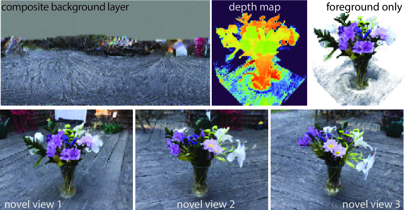
Figure 5. Qualitative results for the real-captured scene extension of ReLU Fields on Flowers. We decompose the scene into a series of spherical-background shells and a foreground ReLU Field layer, which are alpha-composited together to give final novel view renderings. The top-left visualization shows the composite of the background spherical shells un-projected onto a 2D image-plane.

4.2. Occupancy Fields

Another application of coordinate-based MLPs is as a representation of (watertight) 3D geometry. Here, we fit a high resolution ground-truth mesh, as a 3D occupancy field [Mescheder et al., 2019] into a ReLU Field. One might want to do this in order to, for example, take advantage of the volumetric-grid structure to learn priors over geometry, something that is harder to do with meshes or coordinate-based MLPs directly.

Occupancy representation

The core ReLU Field representation used for this application only differs from the radiance fields setup (see Sec. 4.1) as follows: First, since we are only interested in geometry, we do not store any SH coefficients on the grid, and simply model volumetric occupancy as a probability from $[0,1]$. Second, as supervision, we use ground truth point-wise occupancy values in 3D (i.e., 1, if the point lies inside the mesh, and 0 otherwise), rather than rendering an image and applying the loss on the rendered image. Finally, since the ground truth occupancy values are binary, we use a binary cross entropy (BCE) loss. Thus, we obtain the optimized grid $G^{*}$ as,

(2) $$G^{*}:=\operatorname{arg\,min}_{G}\sum_{\mathbf{x}\in\mathcal{B}}\text{BCE}(O(\mathbf{x}),\textsc{ReluField3D}(\tanh(G),\mathbf{x}))$$

where, $O$ is the ground truth occupancy, $\mathbf{x}$ denote sample locations inside an axis-aligned bounding box $\mathcal{B}$, BCE denotes the binary cross entropy loss, and $G$ represents the ReLU Field grid. Note that we use the $\tanh$ to limit the grid values in $(-1,1)$, although other bounding functions, or tensor-normalizations can be used.

We initialize the grid with uniform random values. The supervision signal comes from sampling random points inside and around the tight AABB of the GT high resolution mesh, and generating the occupancy values for those points by doing an inside-outside test on the fly during training. For rendering, we directly show the depth rendering of the obtained occupancy values. We define the grid-extent and the voxel size by obtaining the AABB ensuring a tight fit around the GT mesh.

Table 2. Evaluation results on modeling 3D geometries as occupancy fields. Metric used is Volumetric-IoU [Mescheder et al., 2019]. The baseline MLP is our implementation of OccupancyNetworks [Mescheder et al., 2019].

	MLP	Grid	ReLUField
Thai Statue	0.867	0.827	0.901
Lucy	0.920	0.883	0.935
Bimba	0.983	0.978	0.987
Grog	0.961	0.947	0.971
Lion	0.956	0.970	0.979
Ramses	0.973	0.961	0.978
Dragon	0.886	0.761	0.896
Average volumetric-IoU	0.935	0.903	0.949

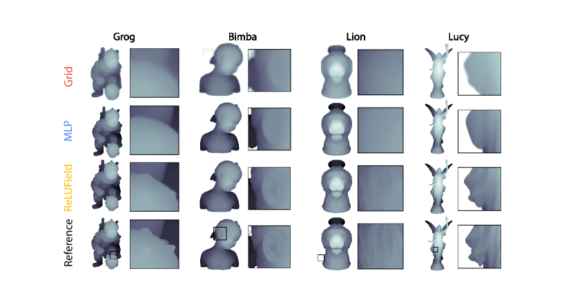
Figure 6. Qualitative results for the occupancy fields comparing Grid, MLP, and ReLUField.

Evaluation

Figure 6 shows the qualitative results of the different representations used for this task. We can see that a ReLUField in this case yields higher quality reconstructions than a standard Grid, or a coordinate-based MLP. Quantitative scores, Volumetric-IoU as used in [Mescheder et al., 2019], for the ThaiStatue, Lucy, Bimba, Grog, Lion, Ramses, and Dragon models are summarized in Tab. 2. ReLUField and Grid require 15 mins, while MLP requires 1.5 hours for training.

5. Discussion

5.1. Limitations

Our approach has some limitations. First, the resulting representations are large. A ReLU Field of size $128^{3}$ used for radiance fields (i.e., with SH coefficients) takes 260Mb, and the large version at $256^{3}$ takes 2.0 Gb of storage. We believe that combining ReLU Field with a sparse data structure would see significant gains in performance and reduction in the memory footprint. However, in this work we emphasize the simplicity of our approach and show that the single non-linearity alone is responsible for a surprising degree of quality improvement.

ReLU Field also cannot model more than one “crease” (i.e., discontinuity) per grid cell. While learned features allow for more complex signals to be represented, they do so at the expense of high compute costs. The purpose of this work is to refocus attention on what is actually required for high fidelity scene reconstruction. We believe that the task definition and data are responsible for the high quality results we are seeing now, and show that traditional approaches can yield good results with minor modifications, and neural networks may not be required. However, this is just one data-point in the space of possible representations, for a given specific task we expect that the optimal representation may be a combination of learned features, neural networks, and discrete signal representations.

5.2. Conclusion

In summary, we presented ReLU Field, an almost embarrassingly simple approach for representing signals; storing unbounded data on N-dimensional grid, and applying a single ReLU after linear interpolation. This change can be incorporated at virtually no computational cost or complexity on top of existing grid-based methods, and strictly improve their representational capability. Our approach contains only values at grid vertices which can be directly optimized via gradient descent; does not rely on any learned parameters, special initialization, or neural networks; and performs comparably with state-of-the-art approaches in only a fraction of the time.

- [1]
- ner [2021] 2021. Nerf-Pytorch. https://github.com/yenchenlin/nerf-pytorch.
- Agus et al. [2010] Marco Agus, Enrico Gobbetti, José Antonio Iglesias Guitián, and Fabio Marton. 2010. Split-Voxel: A Simple Discontinuity-Preserving Voxel Representation for Volume Rendering.. In VG@ Eurographics. 21–28.
- Aliev et al. [2020] Kara-Ali Aliev, Artem Sevastopolsky, Maria Kolos, Dmitry Ulyanov, and Victor Lempitsky. 2020. Neural Point-Based Graphics. arXiv:cs.CV/1906.08240
- Attal et al. [2020] Benjamin Attal, Selena Ling, Aaron Gokaslan, Christian Richardt, and James Tompkin. 2020. Matryodshka: Real-time 6dof video view synthesis using multi-sphere images. In European Conference on Computer Vision. Springer, 441–459.
- Bala et al. [2003] Kavita Bala, Bruce Walter, and Donald P Greenberg. 2003. Combining edges and points for interactive high-quality rendering. ACM Transactions on Graphics (TOG) 22, 3 (2003), 631–640.
- Billingsley [1966] Fred C Billingsley. 1966. Processing ranger and mariner photography. Optical Engineering 4, 4 (1966), 404147.
- Chan et al. [2021a] Eric R. Chan, Connor Z. Lin, Matthew A. Chan, Koki Nagano, Boxiao Pan, Shalini De Mello, Orazio Gallo, Leonidas Guibas, Jonathan Tremblay, Sameh Khamis, Tero Karras, and Gordon Wetzstein. 2021a. Efficient Geometry-aware 3D Generative Adversarial Networks. arXiv:cs.CV/2112.07945
- Chan et al. [2021b] Eric R Chan, Marco Monteiro, Petr Kellnhofer, Jiajun Wu, and Gordon Wetzstein. 2021b. pi-gan: Periodic implicit generative adversarial networks for 3d-aware image synthesis. In IEEE CVPR. 5799–5809.
- Chen et al. [2020] Yinbo Chen, Sifei Liu, and Xiaolong Wang. 2020. Learning Continuous Image Representation with Local Implicit Image Function. CoRR abs/2012.09161 (2020).
- Chen and Zhang [2019] Zhiqin Chen and Hao Zhang. 2019. Learning implicit fields for generative shape modeling. In Proceedings of the IEEE/CVF Conference on Computer Vision and Pattern Recognition. 5939–5948.
- Garbin et al. [2021] Stephan J Garbin, Marek Kowalski, Matthew Johnson, Jamie Shotton, and Julien Valentin. 2021. Fastnerf: High-fidelity neural rendering at 200fps. arXiv preprint arXiv:2103.10380 (2021).
- Groueix et al. [2018] Thibault Groueix, Matthew Fisher, Vladimir G. Kim, Bryan C. Russell, and Mathieu Aubry. 2018. AtlasNet: A Papier-Mâché Approach to Learning 3D Surface Generation. CoRR abs/1802.05384 (2018).
- Hedman et al. [2021] Peter Hedman, Pratul P Srinivasan, Ben Mildenhall, Jonathan T Barron, and Paul Debevec. 2021. Baking Neural Radiance Fields for Real-Time View Synthesis. arXiv preprint arXiv:2103.14645 (2021).
- Henzler et al. [2019] Philipp Henzler, Niloy J Mitra, and Tobias Ritschel. 2019. Escaping plato’s cave: 3d shape from adversarial rendering. In ICCV. 9984–9993.
- Jiang et al. [2020] Chiyu Jiang, Avneesh Sud, Ameesh Makadia, Jingwei Huang, Matthias Nießner, and Thomas Funkhouser. 2020. Local Implicit Grid Representations for 3D Scenes. In Proceedings of the IEEE Conference on Computer Vision and Pattern Recognition.
- Karras et al. [2018] Tero Karras, Timo Aila, Samuli Laine, and Jaakko Lehtinen. 2018. Progressive Growing of GANs for Improved Quality, Stability, and Variation. In International Conference on Learning Representations. https://openreview.net/forum?id=Hk99zCeAb
- Kingma and Ba [2014] Diederik P Kingma and Jimmy Ba. 2014. Adam: A method for stochastic optimization. arXiv preprint arXiv:1412.6980 (2014).
- Laine and Karras [2010] Samuli Laine and Tero Karras. 2010. Efficient sparse voxel octrees. IEEE Transactions on Visualization and Computer Graphics 17, 8 (2010), 1048–1059.
- Liu et al. [2020] Lingjie Liu, Jiatao Gu, Kyaw Zaw Lin, Tat-Seng Chua, and Christian Theobalt. 2020. Neural Sparse Voxel Fields. NeurIPS (2020).
- Loviscach [2005] Jörn Loviscach. 2005. Efficient magnification of bi-level textures. In ACM SIGGRAPH 2005 Sketches. 131–es.
- Martel et al. [2021] Julien N. P. Martel, David B. Lindell, Connor Z. Lin, Eric R. Chan, Marco Monteiro, and Gordon Wetzstein. 2021. ACORN: Adaptive Coordinate Networks for Neural Scene Representation. arXiv:cs.CV/2105.02788
- Max [1995] Nelson Max. 1995. Optical models for direct volume rendering. IEEE Transactions on Visualization and Computer Graphics 1, 2 (1995), 99–108.
- Mescheder et al. [2019] Lars Mescheder, Michael Oechsle, Michael Niemeyer, Sebastian Nowozin, and Andreas Geiger. 2019. Occupancy networks: Learning 3d reconstruction in function space. In Proceedings of the IEEE/CVF Conference on Computer Vision and Pattern Recognition. 4460–4470.
- Mildenhall et al. [2020] Ben Mildenhall, Pratul P Srinivasan, Matthew Tancik, Jonathan T Barron, Ravi Ramamoorthi, and Ren Ng. 2020. Nerf: Representing scenes as neural radiance fields for view synthesis. In ECCV. 405–421.
- Müller et al. [2022] Thomas Müller, Alex Evans, Christoph Schied, and Alexander Keller. 2022. Instant Neural Graphics Primitives with a Multiresolution Hash Encoding. arXiv:2201.05989 (Jan. 2022).
- Nguyen-Phuoc et al. [2019] Thu Nguyen-Phuoc, Chuan Li, Lucas Theis, Christian Richardt, and Yong-Liang Yang. 2019. Hologan: Unsupervised learning of 3d representations from natural images. In ICCV. 7588–7597.
- Nguyen-Phuoc et al. [2020] Thu Nguyen-Phuoc, Christian Richardt, Long Mai, Yong-Liang Yang, and Niloy J. Mitra. 2020. BlockGAN: Learning 3D Object-aware Scene Representations from Unlabelled Images. CoRR abs/2002.08988 (2020). https://arxiv.org/abs/2002.08988
- Niemeyer and Geiger [2021] Michael Niemeyer and Andreas Geiger. 2021. Giraffe: Representing scenes as compositional generative neural feature fields. In IEEE CVPR. 11453–11464.
- Parilov and Zorin [2008] Evgueni Parilov and Denis Zorin. 2008. Real-time rendering of textures with feature curves. ACM Transactions on Graphics (TOG) 27, 1 (2008), 1–15.
- Park et al. [2019] Jeong Joon Park, Peter Florence, Julian Straub, Richard Newcombe, and Steven Lovegrove. 2019. Deepsdf: Learning continuous signed distance functions for shape representation. In Proceedings of the IEEE/CVF Conference on Computer Vision and Pattern Recognition. 165–174.
- Pavić and Kobbelt [2010] Darko Pavić and Leif Kobbelt. 2010. Two-Colored Pixels. In Computer Graphics Forum, Vol. 29. Wiley Online Library, 743–752.
- Ramanarayanan et al. [2004] Ganesh Ramanarayanan, Kavita Bala, and Bruce Walter. 2004. Feature-based textures.
- Reiser et al. [2021] Christian Reiser, Songyou Peng, Yiyi Liao, and Andreas Geiger. 2021. KiloNeRF: Speeding up Neural Radiance Fields with Thousands of Tiny MLPs. arXiv preprint arXiv:2103.13744 (2021).
- Schonberger and Frahm [2016] Johannes L Schonberger and Jan-Michael Frahm. 2016. Structure-from-motion revisited. In IEEE CVPR. 4104–4113.
- Schwarz et al. [2020] Katja Schwarz, Yiyi Liao, Michael Niemeyer, and Andreas Geiger. 2020. Graf: Generative radiance fields for 3d-aware image synthesis. arXiv preprint arXiv:2007.02442 (2020).
- Sen [2004] Pradeep Sen. 2004. Silhouette maps for improved texture magnification. In Proceedings of the ACM SIGGRAPH/EUROGRAPHICS conference on Graphics hardware. 65–73.
- Sen et al. [2003] Pradeep Sen, Mike Cammarano, and Pat Hanrahan. 2003. Shadow silhouette maps. ACM Transactions on Graphics (TOG) 22, 3 (2003), 521–526.
- Sitzmann et al. [2020] Vincent Sitzmann, Julien N. P. Martel, Alexander W. Bergman, David B. Lindell, and Gordon Wetzstein. 2020. Implicit Neural Representations with Periodic Activation Functions. arXiv:cs.CV/2006.09661
- Sitzmann et al. [2019] Vincent Sitzmann, Justus Thies, Felix Heide, Matthias Nießner, Gordon Wetzstein, and Michael Zollhöfer. 2019. DeepVoxels: Learning Persistent 3D Feature Embeddings. arXiv:cs.CV/1812.01024
- Sun et al. [2021] Cheng Sun, Min Sun, and Hwann-Tzong Chen. 2021. Direct Voxel Grid Optimization: Super-fast Convergence for Radiance Fields Reconstruction. arXiv:cs.CV/2111.11215
- Tarini and Cignoni [2005] Marco Tarini and Paolo Cignoni. 2005. Pinchmaps: Textures with customizable discontinuities. In Computer Graphics Forum, Vol. 24. Blackwell Publishing, Inc Oxford, UK and Boston, USA, 557–568.
- Tulsiani et al. [2017] Shubham Tulsiani, Tinghui Zhou, Alexei A Efros, and Jitendra Malik. 2017. Multi-view supervision for single-view reconstruction via differentiable ray consistency. In Proceedings of the IEEE conference on computer vision and pattern recognition. 2626–2634.
- Tumblin and Choudhury [2004] Jack Tumblin and Prasun Choudhury. 2004. Bixels: Picture samples with sharp embedded boundaries.. In Rendering Techniques. Citeseer, 255–264.
- Wizadwongsa et al. [2021] Suttisak Wizadwongsa, Pakkapon Phongthawee, Jiraphon Yenphraphai, and Supasorn Suwajanakorn. 2021. Nex: Real-time view synthesis with neural basis expansion. In Proceedings of the IEEE/CVF Conference on Computer Vision and Pattern Recognition. 8534–8543.
- Yu et al. [2021a] Alex Yu, Sara Fridovich-Keil, Matthew Tancik, Qinhong Chen, Benjamin Recht, and Angjoo Kanazawa. 2021a. Plenoxels: Radiance Fields without Neural Networks. arXiv:cs.CV/2112.05131
- Yu et al. [2021b] Alex Yu, Ruilong Li, Matthew Tancik, Hao Li, Ren Ng, and Angjoo Kanazawa. 2021b. Plenoctrees for real-time rendering of neural radiance fields. arXiv preprint arXiv:2103.14024 (2021).
- Zhang et al. [2018] Richard Zhang, Phillip Isola, Alexei A Efros, Eli Shechtman, and Oliver Wang. 2018. The unreasonable effectiveness of deep features as a perceptual metric. In Proceedings of the IEEE conference on computer vision and pattern recognition. 586–595.