Policy-based Primal-Dual Methods for Convex Constrained Markov Decision Processes

Abstract

We study convex Constrained Markov Decision Processes (CMDPs) in which the objective is concave and the constraints are convex in the state-action occupancy measure. We propose a policy-based primal-dual algorithm that updates the primal variable via policy gradient ascent and updates the dual variable via projected sub-gradient descent. Despite the loss of additivity structure and the nonconvex nature, we establish the global convergence of the proposed algorithm by leveraging a hidden convexity in the problem, and prove the $\mathcal{O}\left(T^{-1/3}\right)$ convergence rate in terms of both optimality gap and constraint violation. When the objective is strongly concave in the occupancy measure, we prove an improved convergence rate of $\mathcal{O}\left(T^{-1/2}\right)$. By introducing a pessimistic term to the constraint, we further show that a zero constraint violation can be achieved while preserving the same convergence rate for the optimality gap. This work is the first one in the literature that establishes non-asymptotic convergence guarantees for policy-based primal-dual methods for solving infinite-horizon discounted convex CMDPs.

1 Introduction

Reinforcement Learning (RL) aims to learn how to map situations to actions so as to maximize the expected cumulative reward. Mathematically, this objective can be rewritten as an inner product between the state-action occupancy measure induced by the policy and a policy-independent reward for each state-action pair. However, many decision-making problems of interests take a form beyond the cumulative reward, such as apprenticeship learning (Abbeel and Ng 2004), diverse skill discovery (Eysenbach et al. 2018), pure exploration (Hazan et al. 2019), and state marginal matching (Lee et al. 2019), among others. Recently, Zhang et al. (2020) and Zahavy et al. (2021) abstract such problems as convex Markov Decision Processes (MDPs), which focus on finding a policy to maximize a concave function of the induced state-action occupancy measure.

However, in many safety-critical applications of convex MDP problems, e.g., in autonomous driving (Fisac et al. 2018), cyber-security (Zhang et al. 2019), and financial management (Abe et al. 2010), the agent is also subject to safety constraints. Nonetheless, the classical safe RL and CMDPs (Altman 1999), which assume that the objective and constraints are linear in the state-action occupancy measure, are not directly applicable to more general convex CMDP problems where the objective and the constraints can respectively be concave and convex in the occupancy measure.

In this paper, we focus on the optimization perspective of convex CMDP problems and aim to develop a principled theory for the direct policy search method. When moving beyond linear structures in the objective and the constraints, we quickly face several technical challenges. Firstly, the convex CMDP problem has a nonconcave objective and the nonconvex constraints with respect to the policy even under the simplest direct policy parameterization. Thus, the existing tools from the convex constrained optimization literature are not applicable. Secondly, as the gradient of the objective/constraint with respect to the occupancy measure becomes policy-dependent, evaluating the single-step improvement of the algorithm becomes harder without knowing the occupancy measure. Yet, evaluating the occupancy measure for a given policy can be inefficient (Tsybakov 2008). Thirdly, the performance difference lemma in Kakade and Langford (2002), which is key to the analysis of the policy-based primal-dual method for the standard CMDP in Ding et al. (2020), is no longer helpful for general convex CMDPs.

In view of the aforementioned challenges, our main contributions to the policy search of convex CMDP problems are summarized in Table 1 and are provided below:

• Despite being nonconvex with respect to the policy and nonlinear with respect to the state-action occupancy measure, we prove that the strong duality still holds for convex CMDP problems under some mild conditions.

• We propose a simple but effective algorithm – Primal-Dual Projected Gradient method (PDPG) – for solving discounted infinite-horizon convex CMDPs. We employ policy gradient ascent to update the primal variable and projected sub-gradient descent to update the dual variable. Strong bounds on the optimality gap and the constraint violations are established for both the concave objective and the the strongly concave objective cases.

• Inspired by the idea of “optimistic pessimism in the face of uncertainty”, we further propose a modified method, named PDPG-0, which can achieve a zero constraint violation while maintaining the same convergence rate.

Algorithm	Objective	Constraint	Optimality Gap	Constraint Violation
PDPG	Concave	Convex	$\mathcal{O}\left(T^{-1/3}\right)$	$\mathcal{O}\left(T^{-1/3}\right)$
PDPG	Strongly concave	Convex	$\mathcal{O}\left(T^{-1/2}\right)$	$\mathcal{O}\left(T^{-1/2}\right)$
PDPG-0	Concave	Convex	$\mathcal{O}\left(T^{-1/3}\right)$	0
PDPG-0	Strongly concave	Convex	$\mathcal{O}\left(T^{-1/2}\right)$	0

Table 1: We summarize our results for general convex CMDPs. Here $T$ is the total number of iterations.

1.1 Related work

Convex MDP

Motivated by emerging applications in RL whose objectives are beyond cumulative rewards (Schaal 1996; Abbeel and Ng 2004; Ho and Ermon 2016; Hazan et al. 2019; Rosenberg and Mansour 2019; Lee et al. 2019), a series of recent works have focused on developing general approaches for convex MDPs. In particular, Zhang et al. (2020) develops a new policy gradient approach called variational policy gradient and establishes the global convergence of the gradient ascent method by exploiting the hidden convexity of the problem. The REINFORCE-based policy gradient and its variance-reduced version are studied in Zhang et al. (2021). Zahavy et al. (2021) transforms the convex MDP problem to a saddle-point problem using Fenchel duality and proposes a meta-algorithm to solve the problem with standard RL techniques. Geist et al. (2021) proves the equivalence between convex MDPs and mean-field games (MFGs) and shows that algorithms for MFGs can be used to solve convex MDPs. However, the above papers only consider the unconstrained RL problem, which may lead to undesired policies in safety-critical applications. Therefore, additional effort is required to deal with the rising safety constraints, and our work addresses this challenge.

CMDP

Our work is also pertinent to policy-based CMDP algorithms (Altman 1999; Borkar 2005; Achiam et al. 2017; Ding and Lavaei 2022; Chow et al. 2017; Efroni, Mannor, and Pirotta 2020). In particular, Ding et al. (2020) develops a natural policy gradient-based primal-dual algorithm and shows that it enjoys an $\mathcal{O}(T^{-1/2})$ global convergence rate regarding both the optimality gap and the constraint violation under the standard soft-max parameterization. Xu, Liang, and Lan (2021) considers a primal-based approach and achieves a similar global convergence rate. More recently, a line of works (Ying, Ding, and Lavaei 2021; Liu et al. 2021a; Li et al. 2021) introduce entropy regularization and obtain improved convergence rates with dual methods. Nonetheless, these papers focus on cumulative rewards/utilities and do not directly generalize to a boarder class of safe RL problems, such as safe imitation learning (Zhou and Li 2018) and safe exploration (Hazan et al. 2019). Beyond CMDPs with cumulative rewards/utilities, Bai et al. (2021) also studies the convex CMDP problem. Their algorithm is based on the randomized linear programming method proposed by Wang (2020) and it exhibits $\widetilde{\mathcal{O}}(1/\epsilon^{2})$ sample complexity. However, as their approach works directly in the space of state-action occupancy measures, it is thus not applicable to more general problems where the state-action spaces are large and a function approximation is needed. In comparison, our work addresses this issue by focusing on the policy-based primal-dual method and adopting a general soft-max policy parameterization.

1.2 Notations

For a finite set $\mathcal{S}$, let $\Delta(\mathcal{S})$ denote the probability simplex over $\mathcal{S}$, and let $\left|\mathcal{S}\right|$ denote its cardinality. When the variable $s$ follows the distribution $\rho$, we write it as $s\sim\rho$. Let $\mathbb{E}[\cdot]$ and $\mathbb{E}[\cdot\mid\cdot]$, respectively, denote the expectation and conditional expectation of a random variable. Let $\mathbb{R}$ denote the set of real numbers. For a vector $x$, we use $x^{\top}$ to denote the transpose of $x$ and use $\langle x,y\rangle$ to denote the inner product $x^{\top}y$. We use the convention that $\|x\|_{1}=\sum_{i}|x_{i}|$, $\|x\|_{2}=\sqrt{\sum_{i}x_{i}^{2}}$, and $\|x\|_{\infty}=\max_{i}|x_{i}|$. For a set $X\subset\mathbb{R}^{p}$, let $\operatorname{cl}(X)$ denote the closure of $X$. Let $\mathcal{P}_{X}$ denote the projection onto $X$, defined as $\mathcal{P}_{X}(y):=\arg\min_{x\in X}\|x-y\|_{2}$. For a matrix $A$, let $\|A\|_{2}$ stand for the spectral norm, i.e., $\|A\|_{2}=\max_{\|x\|_{2}\neq 0}\left\{\|Ax\|_{2}/\|x\|_{2}\right\}$. For a function $f(x)$, let $\operatorname{arg}\min f(x)$ (resp. $\operatorname{arg}\max f(x)$) denote any global minimum (resp. global maximum) of $f(x)$ and let $\nabla_{x}f(x)$ denote its gradient with respect to $x$.

2 Problem Formulation

Standard CMDP

Consider an infinite-horizon CMDP over a finite state space $\mathcal{S}$ and a finite action space $\mathcal{A}$ with a discount factor $\gamma\in[0,1)$. Let $\rho$ be the initial distribution. The transition dynamics is given by $\mathbb{P}:\mathcal{S}\times\mathcal{A}\rightarrow\Delta(\mathcal{S})$, where $\mathbb{P}(s^{\prime}|s,a)$ is the probability of transition from state $s$ to state $s^{\prime}$ when action $a$ is taken. A policy is a function $\pi:\mathcal{S}\rightarrow\Delta(\mathcal{A})$ that represents the decision rule that the agent uses, i.e., the agent takes action $a$ with probability $\pi(a|s)$ in state $s$. We denote the set of all stochastic policies as $\Pi$. The goal of the agent is to find a policy that maximizes some long-term objective. In standard CMDPs, the agent aims at maximizing the expected (discounted) cumulative reward for a given initial distribution $\rho$ while satisfying constraints on the expected (discounted) cumulative cost, i.e.,

$$\max_{\pi\in\Pi} V^{\pi}(r):=\mathbb{E}\left[\sum_{k=0}^{\infty}\gamma^{k}r\left(s_{k},a_{k}\right)\bigg{|}\pi,s_{0}\sim\rho\right],$$ (1)

s.t. $$V^{\pi}(c):=\mathbb{E}\left[\sum_{k=0}^{\infty}\gamma^{k}c\left(s_{k},a_{k}\right)\bigg{|}\pi,s_{0}\sim\rho\right]\leq 0,$$

where the expectation is taken over all possible trajectories such that , and $r(\cdot,\cdot)$ and $c(\cdot,\cdot)$ denote the reward and cost functions, respectively. For given reward function $r(\cdot,\cdot)$, we define the state-action value function (Q-function) under policy $\pi$ as

$$Q^{\pi}(r;s,a):=\mathbb{E}\left[\sum_{k=0}^{\infty}\gamma^{k}r\left(s_{k},a_{k}\right)\bigg{|}\pi,s_{0}=s,a_{0}=a\right],$$ (2)

which can be interpreted as the expected total reward with an initial state $s_{0}=s$ and an initial action $a_{0}=a$. For each policy $\pi\in\Pi$ and state-action pair $(s,a)\in\mathcal{S}\times\mathcal{A}$, the discounted state-action occupancy measure is defined as

$$\lambda^{\pi}(s,a)=(1-\gamma)\sum_{k=0}^{\infty}\gamma^{k}\mathbb{P}\left(s_{k}=s,a_{k}=a\mid\pi,s_{0}\sim\rho\right).$$ (3)

We use $\Lambda$ to denote the set of all possible state-action occupancy measures, which is a convex polytope (cf. (26)). By using $\lambda$ as decision variables, the CMDP problem in (1) can be re-parameterized as follows:

$$\max_{\lambda\in\Lambda}\frac{1}{1-\gamma}\langle r,\lambda\rangle,\quad\text{s.t.}\quad\frac{1}{1-\gamma}\langle c,\lambda\rangle\leq 0.$$ (4)

This is known as the linear programming formulation of the CMDP (Altman 1999). Once a solution $\lambda^{\star}$ is computed, the corresponding policy can be recovered using the relation $\pi(a|s)=\lambda^{\pi}(s,a)/\sum_{a^{\prime}\in\mathcal{A}}\lambda^{\pi}(s,a^{\prime})$.

Convex CMDP

In this work, we consider a more general problem where the agent’s goal is to find a policy that maximizes a concave function of the state-action occupancy measure $\lambda$ subject to a single convex constraint on $\lambda$, namely

$$\underset{\lambda\in\Lambda}{\max}\ f(\lambda)\quad\text{s.t.}\quad{g}(\lambda)\leq{0},$$ (5)

where $f$ is concave and ${g}$ is convex. As (5) is a convex program in $\lambda$, we refer to the problem as Convex CMDP. We emphasize that the method proposed in this paper directly generalizes to multiple constraints and we present the single constraint setting only for brevity.

Example 2.1 (Safety-aware apprenticeship learning (AL))

In AL, instead of maximizing the long-term reward, the agent learns to mimic an expert’s demonstrations. When there are critical safety requirements, the learner will also strive to satisfy given constraints on the expected total cost (Zhou and Li 2018). This problem can be formulated as

$$\underset{\lambda\in\Lambda}{\max}\ f(\lambda)=-\operatorname{dist}(\lambda,\lambda_{e})\ \ \text{s.t.}\ g(\lambda)=\dfrac{1}{1-\gamma}\langle c,\lambda\rangle\leq{0},$$ (6)

where $\lambda_{e}$ corresponds to the expert demonstration, $c$ denotes the cost function, and $\operatorname{dist}(\cdot,\cdot)$ can be any distance function on $\Lambda$, e.g., $\ell^{2}$-distance or Kullback-Liebler (KL) divergence.

Example 2.2 (Feasibility constrained MDPs)

As an extension to standard CMDPs, the designer may desire to control the MDP through more general constraints described by a convex feasibility region $C$ (Miryoosefi et al. 2019) (e.g., a single point representing a known safe policy) such that the learned policy is not too far away from $C$. In this case, the problem can be cast as

$$\underset{\lambda\in\Lambda}{\max}\ f(\lambda)=\dfrac{1}{1-\gamma}\langle r,\lambda\rangle\ \ \text{s.t.}\ g(\lambda)=\operatorname{dist}(\lambda,C)\leq d_{0},$$ (7)

where $d_{0}\geq 0$ denotes the threshold of the allowable deviation.

Policy Parameterization

Since recovering a policy from its corresponding state-action occupancy measure is toilless, a natural approach to solving the convex CMDP problem is to optimize (5) directly (or equivalently (4) for standard CMDPs). However, since the decision variable $\lambda$ has the size ${|\mathcal{S}||\mathcal{A}|}$, such approaches lack scalability and converge extremely slowly for large state and action spaces. In this work, we consider the direct policy search method, which can handle the curse of dimensionality via the policy parameterization. We assume that policy $\pi=\pi_{\theta}$ is parameterized by a general soft-max function, meaning that

$$\pi_{\theta}(a|s)=\frac{\exp\{\psi(\theta;s,a)\}}{\sum_{a^{\prime}\in\mathcal{A}}\exp\left\{\psi\left(\theta;s,a^{\prime}\right)\right\}},\ \forall\ (s,a)\in\mathcal{S}\times\mathcal{A},$$ (8)

where $\psi(\cdot\ ;s,a)$ is some smooth function, $\theta\in\Theta$ is the parameter vector, and $\Theta$ is a convex feasible set. We assume that $\theta$ over-parameterizes the set of all stochastic policies in the sense that $\operatorname{cl}\left(\lambda(\Theta)\right)=\Lambda$. Further assumptions on the parameterization will be formally stated in Section 4. In practice, the function $\psi$ can be chosen to be a deep neural network, where $\theta$ is the parameter and the state-action pair $(s,a)$ is the input. Under parameterization (8), problem (5) can be re-written as

$$\max_{\theta\in\Theta}F(\theta):=f(\lambda(\theta))\quad\text{s.t.}\quad G(\theta):=g(\lambda(\theta))\leq 0,$$ (9)

where we use the shorthand notations $\lambda(\theta):=\lambda^{\pi_{\theta}}$ and $\lambda(\theta;s,a):=\lambda^{\pi_{\theta}}(s,a)$. It is worth mentioning that (9) is a nonconvex problem due to its nonconcave objective function and nonconvex constraints with respect to $\theta$.

Lagrangian Duality

Consider the Lagrangian function associated with (9), ${\mathcal{L}}(\theta,\mu):=F(\theta)-\mu G(\theta)$. For the ease of theoretical analysis, we define $L(\lambda,\mu):=f(\lambda)-\mu g\left(\lambda\right)$, which is concave in $\lambda$ when $\mu\geq{0}$. It is clear that ${\mathcal{L}}(\theta,\mu)=L(\lambda(\theta),\mu)$. The dual function is defined as $\mathcal{D}(\mu):=\max_{\theta\in\Theta}{\mathcal{L}}(\theta,\mu)$. Let $\pi_{\theta^{\star}}$ be the optimal policy such that $\theta^{\star}$ is the optimal solution to (9), and $\mu^{\star}$ be the optimal dual variable.

In constrained optimization, strict feasibility can induce many desirable properties. Assume that the following Slater’s condition holds.

Assumption 2.1 (Slater’s condition)

There exist $\widetilde{\theta}\in\Theta$ and $\xi>{0}$ such that ${G}(\widetilde{\theta})=g(\lambda({\widetilde{\theta}}))\leq-\xi$.

The Slater’s condition is a standard assumption and it holds when the feasible region has an interior point. In practice, such a point is often easy to find using prior knowledge of the problem. The following result is a direct consequence of the Slater’s condition (Altman 1999).

Lemma 2.2 (Strong duality and boundedness of $\mu^{\star}$)

Let Assumption 2.1 hold and suppose that $\operatorname{cl}\left(\lambda(\Theta)\right)=\Lambda$. Then,

(I) $F\left(\theta^{\star}\right)=\mathcal{D}\left(\mu^{\star}\right)=\mathcal{L}\left(\theta^{\star},\mu^{\star}\right)$,

(II) $0\leq\mu^{\star}\leq(F(\theta^{\star})-F(\widetilde{\theta}))/\xi$.

For completeness, we provide a proof for Lemma 2.2 in Appendix A. The strong duality implies that (9) is equivalent to the following saddle point problem:

$$\max_{\theta\in\Theta}\min_{\mu\geq 0}{\mathcal{L}}(\theta,\mu)=\min_{\mu\geq 0}\max_{\theta\in\Theta}{\mathcal{L}}(\theta,\mu).$$ (10)

Motivated by this equivalence, we seek to develop a primal-dual algorithm to solve the problem.

3 Safe Policy Search Beyond Cumulative Rewards/Utilities

To solve (10), we propose the following Primal-Dual Projected Gradient Algorithm (PDPG):

$$\left\{\begin{aligned} \theta^{t+1}&=\mathcal{P}_{\Theta}\left(\theta^{t}+\eta_{1}\nabla_{\theta}{\mathcal{L}}(\theta^{t},\mu^{t})\right)\\ \mu^{t+1}&=\mathcal{P}_{U}\left(\mu^{t}-\eta_{2}\nabla_{\mu}{\mathcal{L}}(\theta^{t},\mu^{t})\right)\end{aligned}\right.,\ t=0,1,\dots$$ (11)

where $\eta_{1}>0$, $\eta_{2}>0$ are constant step-sizes, and the dual feasible region $U:=[0,C_{0}]$ is an interval that contains $\mu^{\star}$. By Lemma 2.2, choosing $C_{0}\geq(F(\theta^{\star})-F(\widetilde{\theta}))/\xi$ satisfies the requirement. The method (11) adopts an alternating update scheme: the primal step performs the projected gradient ascent in the policy space, whereas dual step updates the multiplier with projected sub-gradient descent such that $\mu^{t+1}$ is obtained by adding a multiple of the constraint violation to $\mu^{t}$. The values of $C_{0}$, $\eta_{1}$, $\eta_{2}$ will be specified later in the paper.

Unlike standard CMDPs (1) where the value function is defined as discounted cumulative rewards/utilities and admits an additive structure, performing and analyzing algorithm (11) are far more challenging for convex CMDPs.

3.1 Gradient Evaluation of the Lagrangian Function

Computing the primal update in (11) involves evaluating the gradient of the Lagrangian with respect to $\theta$, i.e., $\nabla_{\theta}{\mathcal{L}}(\theta,\mu)=\nabla_{\theta}\left[f(\lambda(\theta))-\mu g(\lambda(\theta))\right]$. When $f(\cdot)$ and $g(\cdot)$ are linear as in the standard CMDP, i.e., $f(\lambda)=\langle r,\lambda\rangle/(1-\gamma)$ and $g(\lambda)=\langle c,\lambda\rangle/(1-\gamma)$, the Lagrangian can be viewed as a value function with reward $r-\mu c$, i.e., ${\mathcal{L}}(\theta,\mu)=V^{\pi_{\theta}}\left(r-\mu c\right)$, so the Policy gradient theorem proposed by Sutton et al. (1999) can be applied (cf. Lemma G.1). However, this favorable result is not applicable when $f(\cdot)$ and $g(\cdot)$ are general concave/convex functions. Instead, we present two alternative approaches below. More details are deferred to Appendix A.1.

Variational Policy Gradient (Zhang et al. 2020)

By leveraging the Fenchel duality, Zhang et al. (2020) showed that the gradient $\nabla_{\theta}{\mathcal{L}}(\theta,\mu)$ can be computed by solving a stochastic saddle point problem, in particular

$$\nabla_{\theta}{\mathcal{L}}(\theta, \mu)=\lim_{\delta\rightarrow 0_{+}}\underset{x}{\operatorname{argmax}}\inf_{z}\bigg{\{}(1-\gamma)\big{[}V^{\pi_{\theta}}(z)$$ (12)

$$+\delta\left\langle\nabla_{\theta}V^{\pi_{\theta}}(z),x\right\rangle\big{]}-L_{*}(z,\mu)-\frac{\delta}{2}\|x\|^{2}\bigg{\}},$$

where $L_{*}(z,\mu):=\inf_{\lambda}\left\{\langle z,\lambda\rangle-L(\lambda,\mu)\right\}$ is the concave conjugate of $L(\lambda,\mu)$ with respect to $\lambda$. As $L_{*}(z,\mu)$ is concave in $z$ and $V^{\pi_{\theta}}(z)=\left\langle z,\lambda(\theta)\right\rangle$ is linear in $z$, the max-min problem in (12) is a concave-convex saddle point problem and can be solved by a simple gradient ascent-descent algorithm.

REINFORCE-based Policy Gradient (Zhang et al. 2021)

By noticing the relation $\nabla_{\theta}V^{\pi_{\theta}}(r)=\left[\nabla_{\theta}\lambda(\theta)\right]^{\top}\cdot r/(1-\gamma)$, one can view $\nabla_{\theta}{\mathcal{L}}(\theta,\mu)$ as the standard policy gradient for the value function with the reward $\nabla_{\lambda}L(\lambda(\theta),\mu)$ (assuming that $f(\lambda)$, $g(\lambda)$, and $\lambda(\theta)$ are all differentiable), i.e.,

$$\nabla_{\theta}{\mathcal{L}}(\theta,\mu) =\left[\nabla_{\theta}\lambda(\theta)\right]^{\top}\cdot\nabla_{\lambda}L(\lambda(\theta),\mu)$$ (13)

$$=(1-\gamma)\nabla_{\theta}V^{\pi_{\theta}}(\nabla_{\lambda}L(\lambda(\theta),\mu)),$$

where the first equality follows from the chain rule. Thus, the gradient $\nabla_{\theta}{\mathcal{L}}(\theta,\mu)$ can be estimated with the REINFORCE algorithm proposed by Williams (1992) as long as we can choose an approximation of $\nabla_{\lambda}L(\lambda(\theta),\mu)$ as the reward.

Since $\nabla_{\mu}{\mathcal{L}}(\theta,\mu)=-G(\theta)=-g(\lambda(\theta))$, performing the dual update (11) requires evaluating the constraint function. In cases where an efficient oracle for computing $g(\lambda(\theta))$ from $\theta$ is not available, we can formulate it as another convex problem using the Fenchel duality to avoid directly estimating the current state-action occupancy measure $\lambda(\theta)$:

$$g(\lambda(\theta)) =\sup_{z}\left\{\langle z,\lambda\rangle-g^{*}(z)\right\}$$ (14)

$$=\sup_{z}\left\{(1-\gamma)V^{\pi_{\theta}}(z)-g^{*}(z)\right\}.$$

where $g^{*}(z):=\sup_{\lambda}\left\{\langle z,\lambda\rangle-g(\lambda)\right\}$ is the convex conjugate of $g(\cdot)$ and we leverage the fact that the biconjugate of a convex function equals itself, i.e., $g^{**}(\lambda):=\sup_{z}\left\{\langle z,\lambda\rangle-g^{*}(z)\right\}=g(\lambda)$. In Appendix A.1, we provide a sample-based pseudocode for algorithm (11).

3.2 Exploiting the Hidden Convexity

By itself, (10) is a nonconvex-linear maximin problem. The existing results for the analysis of the gradient ascent descent method (11) for such problems can only guarantee to find a $\epsilon$-stationary point in $\mathcal{O}(\epsilon^{-6})$ iterations (Lin, Jin, and Jordan 2020). To obtain an improved convergence rate and achieve a global optimality, it is necessary to exploit the “hidden convexity” of (9) with respect to $\lambda$.

However, standard analyses based on the performance difference lemma (cf. Lemma G.4) do not apply to convex CMDPs (Agarwal et al. 2021; Ding et al. 2020). A key insight is that, due to the loss of linearity, the performance difference lemma together with concavity can only provide an upper bound for the single-step improvement with the gradient information at the current step (more details can be found in Appendix A.2). Thus, this prompts us to introduce a new analysis to bound the average performance in terms of the Lagrangian (cf. (16)).

Motivated by Zhang et al. (2020), we leverage the fact that the primal update implies the formula

$${\mathcal{L}}(\theta^{t+1},\mu^{t})=\underset{{\theta\in\Theta}}{\operatorname{max}}\ \bigg{\{}{\mathcal{L}}(\theta^{t},\mu^{t})+(\theta- \theta^{t})^{\top}\nabla_{\theta}{\mathcal{L}}(\theta^{t},\mu^{t})$$ (15)

$$-\frac{1}{2\eta_{1}}\|\theta-\theta^{t}\|_{2}^{2}\bigg{\}}.$$

With a proper step-size $\eta_{1}$, (15) guarantees a strict single-step improvement. The basis of our analysis lies in designing a special point $\theta$ from $\theta^{t}$ and $\theta^{\star}$ to lower-bound ${\mathcal{L}}(\theta^{t+1},\mu^{t})$ through (15). The hidden convexity of (9) with respect to $\lambda$ plays a central role in bounding the improvement ${\mathcal{L}}(\theta^{t+1},\mu^{t})-{\mathcal{L}}(\theta^{t},\mu^{t})$ and relating it to the sub-optimality gap ${\mathcal{L}}(\theta^{\star},\mu^{t})-{\mathcal{L}}(\theta^{t},\mu^{t})$. The details are postponed to Section 4.

4 Convergence Analysis

In this section, we establish the global convergence of the primal-dual projected gradient algorithm (11) by exploiting the hidden convexity of (9) with respect to $\lambda$. We refer the reader to the supplement in Appendix B for the proofs of this section.

First, we formally state our assumption about the parameterization (8). To avoid introducing an additional bias, it is natural to assume that the parameterization has enough expressibility to represent any policy, i.e., $\forall\pi\in\Pi$, $\exists\theta\in\Theta$ such that $\pi=\pi_{\theta}$. However, assuming a one-to-one correspondence between $\pi\in\Pi$ and $\pi_{\theta},\theta\in\Theta$ is too restrictive. In practice, using a deep neural network to represent the policy can often arrive at an over-parameterization. Therefore, following Zhang et al. (2021), we assume that $\pi_{\theta}$ is defined such that it can represent any policy and that $\lambda(\cdot)$ is locally continuously invertible. A more detailed discussion can be found in Appendix D.

Assumption 4.1 (Parameterization)

The policy parameterization $\pi=\pi_{\theta}$ over-parameterizes the set of all stochastic policies and satisfies:

(I) For every $\theta\in\Theta$, there exists a neighborhood $\mathcal{U}_{\theta}\ni\theta$ such that the restriction of $\lambda(\cdot)$ to $\mathcal{U}_{\theta}$ is a bijection between $\mathcal{U}_{\theta}$ and $\mathcal{V}_{\lambda(\theta)}:=\lambda(\mathcal{U}_{\theta})$;

(II) Let $\lambda^{-1}_{\mathcal{V}_{\lambda(\theta)}}:\mathcal{V}_{\lambda(\theta)}\rightarrow\mathcal{U}_{\theta}$ be the local inverse of $\lambda(\cdot)$, i.e., $\lambda^{-1}_{\mathcal{V}_{\lambda(\theta)}}(\lambda(\theta_{0}))=\theta_{0},\ \forall\theta_{0}\in\mathcal{U}_{\theta}$. Then, there exists a universal constant $\ell_{\Theta}$ such that $\lambda^{-1}_{\mathcal{V}_{\lambda(\theta)}}$ is $\ell_{\Theta}$-Lipschitz continuous for all $\theta\in\Theta$;

(III) There exists $\bar{\varepsilon}>0$ such that $(1-\varepsilon)\lambda(\theta)+\varepsilon\lambda(\theta^{\star})\in\mathcal{V}_{\lambda(\theta)},\ \forall\varepsilon\leq\bar{\varepsilon},\ \forall\theta\in\Theta$.

We also make the following assumption about the smoothness of the objective and constraint functions.

Assumption 4.2 (Smoothness)

$F(\theta)$ is $\ell_{F}$-smooth with respect to (w.r.t.) $\theta$ and $G(\theta)$ is $\ell_{G}$-smooth w.r.t. $\theta$, i.e., $\|\nabla_{\theta}F(\theta_{1})-\nabla_{\theta}F(\theta_{2})\|_{2}\leq\ell_{F}\|\theta_{1}-\theta_{2}\|_{2}$ and $\|\nabla_{\theta}G(\theta_{1})-\nabla_{\theta}G(\theta_{2})\|_{2}\leq\ell_{G}\|\theta_{1}-\theta_{2}\|_{2}$, $\forall\ \theta_{1},\theta_{2}\in\Theta$.

In optimization, smoothness is important when analyzing the convergence rate of an algorithm. In Appendix E, we provide a discussion which shows that Assumption 4.2 is mild in the sense that if $f(\lambda)$ is smooth with respect to $\lambda$, then $F(\theta)=f(\lambda(\theta))$ is smooth with respect to $\theta$ under some regularity conditions.

The following property about ${\mathcal{L}}(\theta,\mu)$ is the direct consequence of Assumption 4.2.

Lemma 4.3

The functions $f(\cdot)$ and $g(\cdot)$ are bounded on $\Lambda$. Define $M_{F}$ and $M_{G}$ such that $|f(\lambda)|\leq M_{F}$ and $|g(\lambda)|\leq M_{G}$, for all $\lambda\in\Lambda$. Then, it holds that $|{\mathcal{L}}(\theta,\mu)|\leq M_{L},\ \forall\ \theta\in\Theta,\mu\in U$, where $M_{L}:=M_{F}+C_{0}M_{G}$. Furthermore, under Assumption 4.2, ${\mathcal{L}}(\cdot,\mu)$ is $\ell_{L}$-smooth on $\Theta$, for all $\mu\in U$, where $\ell_{L}:=\ell_{F}+C_{0}\ell_{G}$.

To quantify the quality of a given solution $\theta$ to (9), the measures we consider are the optimality gap $F(\theta^{\star})-F(\theta)$ and the constrained violation $\left[G(\theta)\right]_{+}$, where $[x]_{+}:=\max\{x,0\}$. Unlike the unconstrained setting where the last-iterate convergence is of more interest, a primal-dual algorithm for constrained optimization often cannot ensure an effective improvement in every iteration due to the change of the multiplier. Therefore, we focus on the global convergence of algorithm (11) in the time-average sense.

We first bound the average performance in terms of the Lagrangian below.

Proposition 4.4

Let Assumptions 4.1 and 4.2 hold and assume that $\varepsilon\leq\bar{\varepsilon}$. Then, for every $T>0$, the iterates $\left\{\left(\theta^{t},\mu^{t}\right)\right\}_{t=0}^{T-1}$ produced by algorithm (11) with $\eta_{1}=1/\ell_{L}$ satisfy

$$\quad\dfrac{1}{T}\sum_{t=0}^{T-1}\left[{\mathcal{L}}(\theta^{\star},\mu^{t})-{\mathcal{L}}(\theta^{t},\mu^{t})\right]$$ (16)

$$\leq\dfrac{{\mathcal{L}}(\theta^{\star},\mu^{0})-{\mathcal{L}}(\theta^{0},\mu^{0})}{\varepsilon T}+2\varepsilon\ell_{L}\ell_{\Theta}^{2}+\dfrac{2\eta_{2}M_{G}^{2}}{\varepsilon}.$$

We remark that by choosing $\varepsilon=T^{-1/3}$ and $\eta_{2}=T^{-2/3}$, the bound (16) given by Proposition 4.4 has the order of $\mathcal{O}\left(T^{-1/3}\right)$. The core idea in proving Proposition 4.4 is that one can relate the primal update (15) to the sub-optimality gap ${\mathcal{L}}(\theta^{\star},\mu^{t})-{\mathcal{L}}(\theta^{t},\mu^{t})$ by leveraging the hidden convexity of (9) with respect to $\lambda$. Then, as $|\mu^{t+1}-\mu^{t}|=\mathcal{O}(\eta_{2})$, we are able to draw a recursion between the sub-optimality gaps for two consecutive periods (cf. (38)).

The average performance in terms of the Lagrangian can be decomposed into the summation of the average optimality gap and the weighted average “constraint violation”, i.e.,

$$\quad\dfrac{1}{T}\sum_{t=0}^{T-1}\left[{\mathcal{L}}(\theta^{\star},\mu^{t})-{\mathcal{L}}(\theta^{t},\mu^{t})\right]$$ (17)

$$=\dfrac{1}{T}\sum_{t=0}^{T-1}\left[F(\theta^{\star})-F(\theta^{t})\right]+\dfrac{1}{T}\sum_{t=0}^{T-1}\mu^{t}\left[G(\theta^{t})-G(\theta^{\star})\right].$$

Since $\theta^{\star}$ must be a feasible solution, the term $\left[G(\theta^{t})-G(\theta^{\star})\right]$ can be interpreted as an approximate of the constraint violation. To obtain separate bounds for the optimality gap and the true constraint violation, we need to decouple the bound for the average performance.

Theorem 4.5 (General concavity)

Let Assumptions 2.1, 4.1, and 4.2 hold. For every $T\geq({\bar{\varepsilon}})^{-3}$, we choose $C_{0}=1+\left(M_{F}-F(\widetilde{\theta})\right)/{\xi}$, $\mu^{0}=0$, $\eta_{1}=1/\ell_{L}$, and $\eta_{2}=T^{-2/3}$. Then, the sequence $\left\{\left(\theta^{t},\mu^{t}\right)\right\}_{t=0}^{T-1}$ generated by algorithm (11) converges with the rate $\mathcal{O}\left(T^{-1/3}\right)$, in particular

$$\dfrac{1}{T}\sum_{t=0}^{T-1}\left[F(\theta^{\star})-F(\theta^{t})\right]\leq\dfrac{2M_{F}+M_{G}^{2}/2}{T^{2/3}}+\dfrac{2\ell_{L}\ell_{\Theta}^{2}+2M_{G}^{2}}{T^{1/3}},$$ (18a)

$$\dfrac{1}{T}\left[\sum_{t=0}^{T-1}G(\theta^{t})\right]_{+}\leq\dfrac{2M_{F}+M_{G}^{2}/2}{T^{2/3}}+\dfrac{2\ell_{L}\ell_{\Theta}^{2}+2M_{G}^{2}+C_{0}^{2}/2}{T^{1/3}}.$$ (18b)

Theorem 4.5 shows that algorithm (11) achieves a global convergence in the average sense such that the optimality gap and the constraint violation decay to zero with the rate $\mathcal{O}\left(T^{-1/3}\right)$. In other words, to obtain an $\mathcal{O}(\epsilon)$-accurate solution, the iteration complexity is $\mathcal{O}(\epsilon^{-3})$. When $f(\cdot)$ and $g(\cdot)$ are linear functions as in standard CMDPs (cf. (1)), Theorem 4.5 matches the rate of the natural policy gradient primal-dual algorithm under the general parameterization (Ding et al. 2020, Theorem 2).

In Theorem 4.5, the dual feasible region $U=[0,C_{0}]$ is set by taking $C_{0}=1+\left(M_{F}-F(\widetilde{\theta})\right)/{\xi}$. By Lemma 2.2, $\mu^{\star}\leq(F(\theta^{\star})-F(\widetilde{\theta}))/\xi\leq C_{0}-1$, which implies that $\widehat{\mu}:=\mu^{\star}+1\in U$. This “slackness” plays an important role when bounding the constraint violation, as we can write $\left[\sum_{t=0}^{T-1}G(\theta^{t})\right]_{+}=\left[(\mu^{\star}-\widehat{\mu})\sum_{t=0}^{T-1}\nabla_{\mu}{\mathcal{L}}(\theta^{t},\mu^{t})\right]_{+}$, where the latter term can be related to the first-order expansion of ${\mathcal{L}}(\theta,\cdot)$ and bounded through the use of telescoping sums.

When the objective function $f(\lambda(\theta))$ is strongly concave with respect to $\lambda$, we can further improve the convergence rate of algorithm 11 by a similar line of analysis. Firstly, we establish the average performance bound in terms of the Lagrangian.

Proposition 4.6

Let Assumptions 4.1 and 4.2 hold. Suppose that $f(\cdot)$ is $\sigma$-strongly concave w.r.t. $\lambda$ on $\Lambda$. Then, for every $T>0$, the iterates $\left\{\left(\theta^{t},\mu^{t}\right)\right\}_{t=0}^{T-1}$ produced by algorithm (11) with $\eta_{1}=1/\ell_{L}$ satisfy

$$\quad\dfrac{1}{T}\sum_{t=0}^{T-1}[{\mathcal{L}}(\theta^{\star},\mu^{t})-{\mathcal{L}}(\theta^{t},\mu^{t})]$$ (19)

$$\leq\dfrac{{\mathcal{L}}(\theta^{T},\mu^{T-1})-{\mathcal{L}}(\theta^{0},\mu^{0})}{\tilde{\varepsilon}T}+\dfrac{\eta_{2}M_{G}^{2}}{\tilde{\varepsilon}},$$

where $\tilde{\varepsilon}:=\min\{\bar{\varepsilon},{\sigma}/{\left(\sigma+2\ell_{\Theta}^{2}\ell_{L}\right)}\}$.

Different from the general concave case (16), the bound (19) does not contain the constant error term $\mathcal{O}(\varepsilon)$. Thus, by choosing $\eta_{2}=T^{-1/2}$, the average performance has the order $\mathcal{O}\left(T^{-1/2}\right)$. In a similar manner as in Theorem 4.5, we can decouple the average performance to bound the optimality gap and constraint violation.

Theorem 4.7 (Strong concavity)

Let Assumptions 2.1, 4.1, and 4.2 hold. Suppose that $f(\cdot)$ is $\sigma$-strongly concave w.r.t. $\lambda$ on $\Lambda$. For every $T>0$, we choose $C_{0}=1+\left(M_{F}-F(\widetilde{\theta})\right)/{\xi}$, $\mu^{0}=0$, $\eta_{1}=1/\ell_{L}$, and $\eta_{2}=T^{-1/2}$. Then, the sequence $\left\{\left(\theta^{t},\mu^{t}\right)\right\}_{t=0}^{T-1}$ generated by algorithm (11) converges with the rate $\mathcal{O}\left(T^{-1/2}\right)$, in particular

$$\dfrac{1}{T}\sum_{t=0}^{T-1}\left[F(\theta^{\star})-F(\theta^{t})\right]\leq\dfrac{M_{L}+M_{F}}{\tilde{\varepsilon}T}+\left(\dfrac{M_{G}^{2}}{\tilde{\varepsilon}}+\dfrac{M_{G}^{2}}{2}\right)\dfrac{1}{\sqrt{T}},$$ (20a)

$$\dfrac{1}{T}\left[\sum_{t=0}^{T-1}G(\theta^{t})\right]_{+}\leq\dfrac{M_{L}+M_{F}}{\tilde{\varepsilon}T}+\left(\dfrac{M_{G}^{2}}{\tilde{\varepsilon}}+\dfrac{M_{G}^{2}+C_{0}^{2}}{2}\right)\dfrac{1}{\sqrt{T}},$$ (20b)

where $\tilde{\varepsilon}:=\min\{\bar{\varepsilon},{\sigma}/{\left(\sigma+2\ell_{\Theta}^{2}\ell_{L}\right)}\}$.

Theorem 4.7 shows that when $f(\cdot)$ is strongly concave, algorithm (11) admits an improved convergence rate of $\mathcal{O}\left(T^{-1/2}\right)$ by taking the dual step-size $\eta_{2}=\mathcal{O}\left(T^{-1/2}\right)$. Equivalently, the iteration complexity is $\mathcal{O}(\epsilon^{-2})$ to compute an $\mathcal{O}(\epsilon)$-accurate solution.

Remark 4.8 (Direct parameterization)

As a special case, the direct parameterization satisfies Assumption 4.1 once there is a universal positive lower bound for the state occupancy measure defined as $d^{\pi}(s)=\sum_{a}\lambda^{\pi}(s,a),\forall s$. Under the direct parameterization, it can be shown that the primal update (15) also enjoys the so-called variational gradient dominance property for standard MDPs (see, e.g., Agarwal et al. (2021, Lemma 4.1)). This evidence gives a clearer intuition of how the hidden convexity enables us to prove the global convergence of algorithm (11). We refer the reader to Appendix F for a detailed discussion.

5 Zero Constraint Violation

(a) Environment.

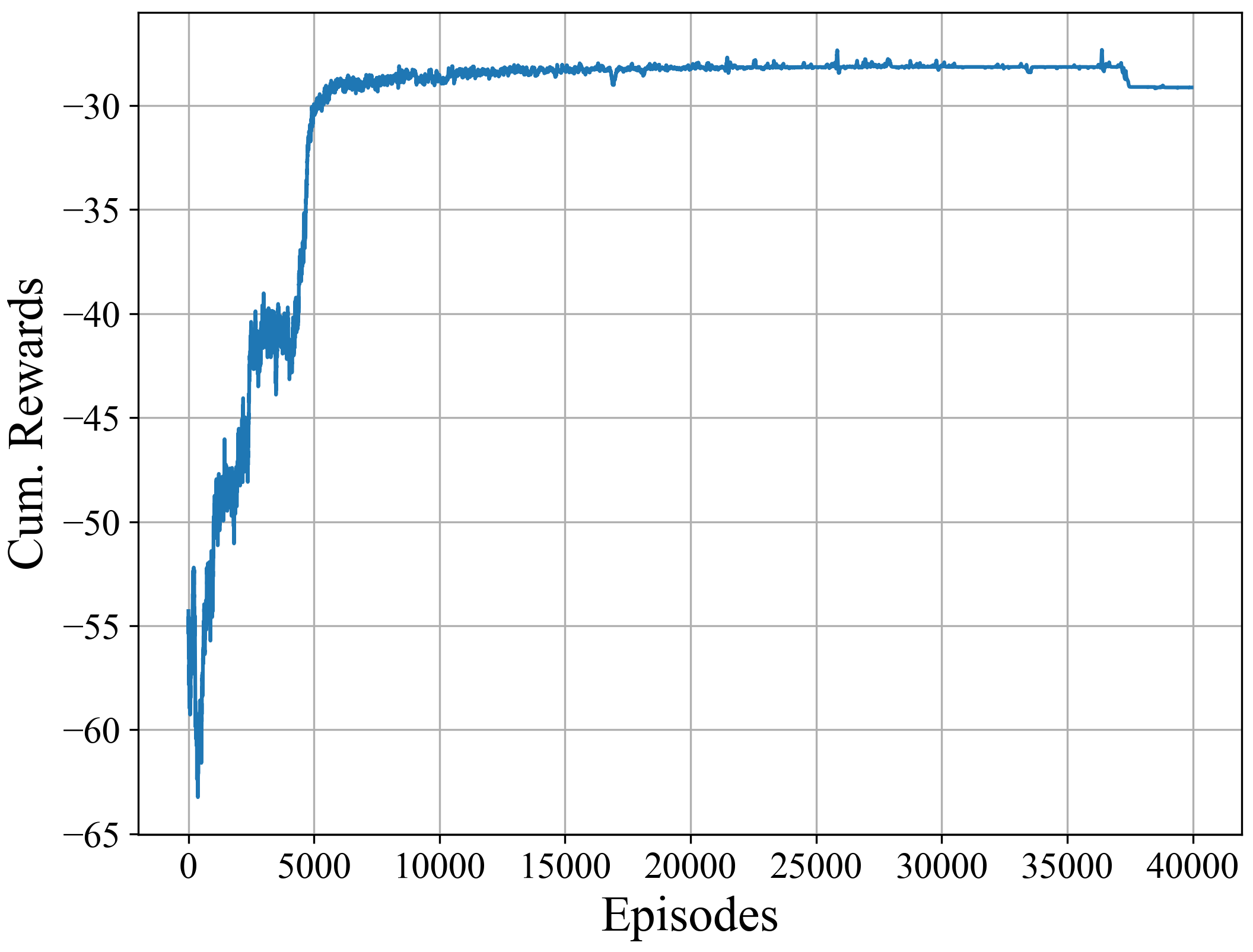
(b) Cumulative reward.

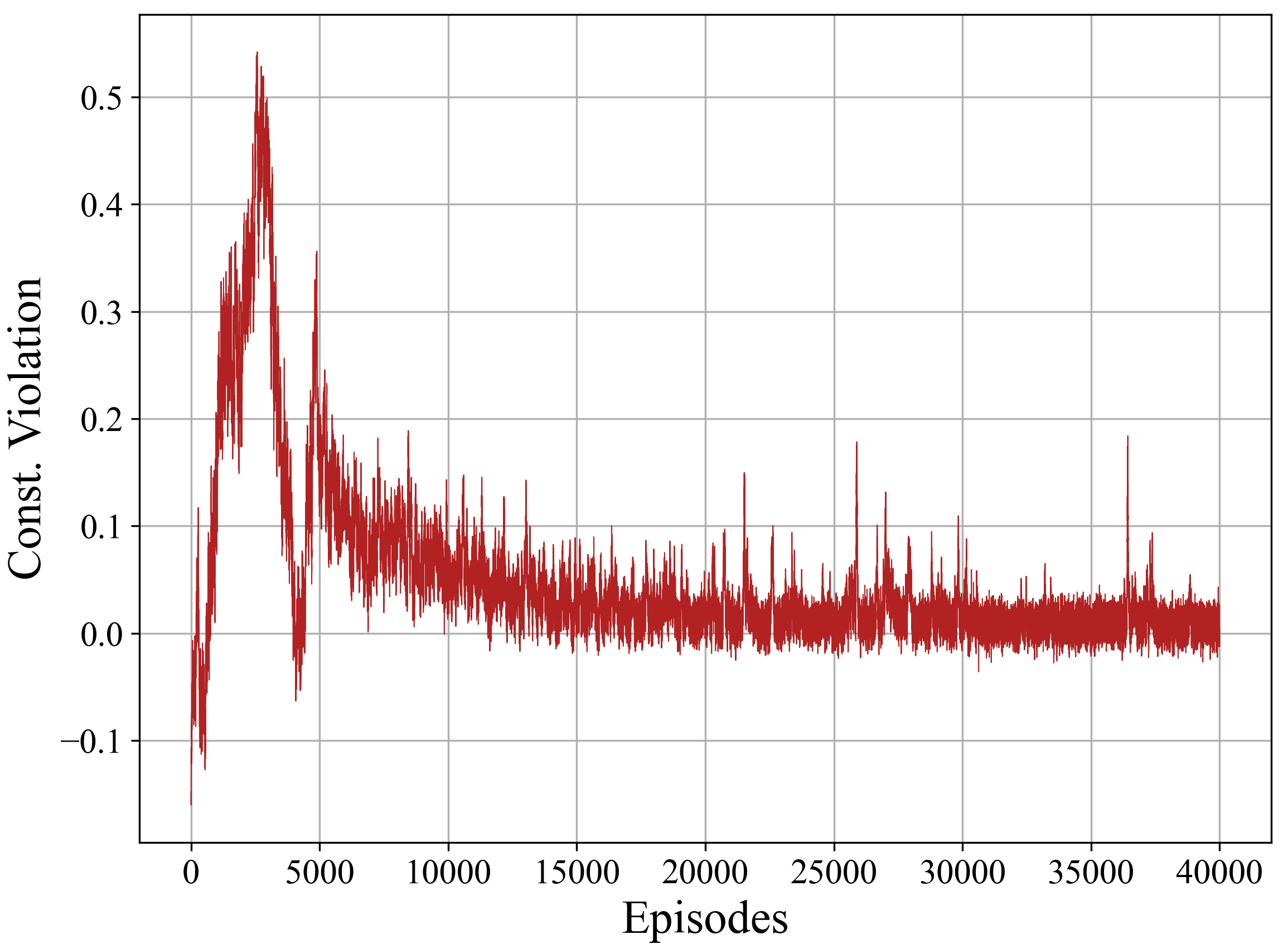
(c) Constraint violation.

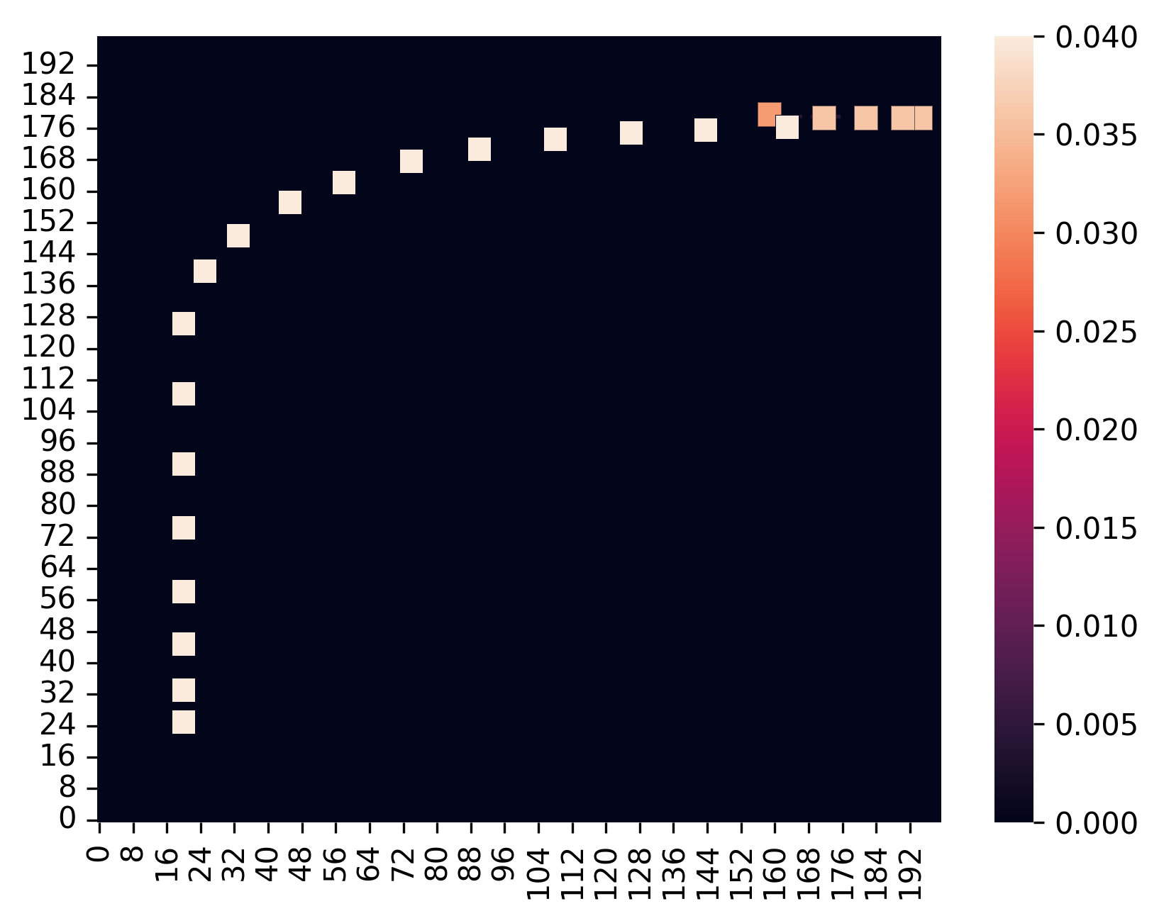
(d) Occupancy measure.

Figure 1: (a) The goal of the agent is to navigate from “S” to “T” while stepping onto the shaded region would incur a penalty. The two paths illustrated by the blue dashed lines represent the two high-reward routes available for the agent. In addition, we enforce a feasibility constraint such that the agent need to satisfy $\|\lambda^{\pi}-\lambda_{0}\|\leq d_{0}$, where $\lambda_{0}$ is the given demonstration corresponding to the red curve in the figure. (b) and (c) Performance of algorithm (11) in terms of cumulative reward and constraint violation with REINFORCE-based policy gradient evaluation on problem (25). (d) Heatmap of the state-action occupancy measure $\lambda^{\pi}$ corresponding to the learned policy $\pi$. It shows that the learned policy chooses one of the high-reward routes which is closed to the given demonstration $\lambda_{0}$. We note that the colored pixels are manually enlarged.

In safety-critical systems where violating the constraint may induce an unexpected cost, having a zero constraint violation is of great importance. Motivated by the recent works (Liu et al. 2021b, a), we will show that a zero constraint violation can be achieved while maintaining the same order of convergence rate for the optimality gap. Consider the pessimistic counterpart of (9):

$$\max_{\theta\in\Theta}F(\theta)=f(\lambda(\theta))\ \text{ s.t. }\ G_{\delta}(\theta):=g(\lambda(\theta))+\delta\leq 0,$$ (21)

where $\delta>0$ is the pessimistic term to be determined. Suppose that $\delta<\xi$, i.e., the pessimistic term is smaller than the strict feasibility of the Slater point, so that the Slater’s condition still holds for problem (21). Consider applying algorithm (11) to problem (21), i.e.,

$$\left\{\begin{aligned} \theta^{t+1}&=\mathcal{P}_{\Theta}\left(\theta^{t}+\eta_{1}\nabla_{\theta}{\mathcal{L}}_{\delta}(\theta^{t},\mu^{t})\right)\\ \mu^{t+1}&=\mathcal{P}_{U}\left(\mu^{t}-\eta_{2}\nabla_{\mu}{\mathcal{L}}_{\delta}(\theta^{t},\mu^{t})\right)\end{aligned}\right.,\ t=0,1,\dots$$ (22)

where ${\mathcal{L}}_{\delta}(\theta,\mu):=F(\theta)-\mu G_{\delta}(\theta)$ is the Lagrangian function for (21). We refer to this variate as the Primal-dual Policy Gradient-Zero Algorithm (PDPG-0). The following theorem states that, with a carefully chosen $\delta$, the constraint violation of the iterates generated by algorithm (22) will be zero for the original problem (9) when $T$ is reasonably large and the optimality gap remains the same order as before. Due to the limit of space, we present an informal version of the theorem below and direct the reader to Appendix C for a detailed statement as well as the proof.

Theorem 5.1

Let Assumptions 2.1, 4.1, and 4.2 hold.

(I) For every reasonably large $T>0$, the sequence $\left\{\left(\theta^{t},\mu^{t}\right)\right\}_{t=0}^{T-1}$ generated by the PDPG-0 algorithm with $\delta=\mathcal{O}(T^{-1/3})$ satisfies

$$\dfrac{1}{T}\sum_{t=0}^{T-1}\left[F(\theta^{\star})-F(\theta^{t})\right]=\mathcal{O}\left(T^{-1/3}\right),\ \dfrac{1}{T}\left[\sum_{t=0}^{T-1}G(\theta^{t})\right]_{+}=0.$$ (23)

(II) When $f(\cdot)$ is $\sigma$-strongly concave w.r.t. $\lambda$ on $\Lambda$, the sequence $\left\{\left(\theta^{t},\mu^{t}\right)\right\}_{t=0}^{T-1}$ generated by the PDPG-0 algorithm with $\delta=\mathcal{O}(T^{-1/2})$ satisfies

$$\dfrac{1}{T}\sum_{t=0}^{T-1}\left[F(\theta^{\star})-F(\theta^{t})\right]=\mathcal{O}(T^{-1/2}),\ \dfrac{1}{T}\left[\sum_{t=0}^{T-1}G(\theta^{t})\right]_{+}=0.$$ (24)

We briefly introduce the ideas behind Theorem 5.1 here. Adding the pessimistic term $\delta$ would shift the optimal solution from $\theta^{\star}$ to another point $\theta_{\delta}^{\star}$. By leveraging the Slater’s condition, we can upper-bound the sub-optimality gap $|F(\theta^{\star})-F(\theta_{\delta}^{\star})|$ by $\mathcal{O}(\delta)$. Since the orders of convergence rates are the same for optimality gap and constraint violation in Theorems 4.5 and 4.7, we can choose $\delta$ to have the same order and then offset the constraint violation for the pessimistic problem (21). As a result, the constraint violation becomes zero for the original problem (9) and the optimality gap preserves its previous order.

6 Numerical Experiment

In this section, we validate algorithm (11) in a feasibility constrained MDP problem (cf. Example 2.2). The experiment is performed on the single agent version of OpenAI Particle environment (Lowe et al. 2017) as illustrated in Figure 1(a).

The state space is continuous and formed by the two-dimensional location of the agent. At each state, there are five actions available to the agent, corresponding to moving leftward, rightward, upward, downward, or staying at the current place. The goal of the agent is to safely navigate from the starting point “S” to the target point “T”. In particular, they will be rewarded as they approach the target and will be penalized when they step onto the unsafe region in the middle. It can be observed from Figure 1(a) that there are two high-reward routes available for the agent as highlighted by the blue dashed lines. Let $\pi_{0}$ be the deterministic policy corresponding to the red curve in Figure 1(a) and $\lambda_{0}$ be the associated state-action occupancy measure. We enforce the feasibility constraint $\|\lambda^{\pi}-\lambda_{0}\|_{2}\leq d_{0}$, where $d_{0}>0$ is the allowable deviation. This constraint means that we want the deviation of the learned policy from the demonstration $\pi_{0}$ is within a threshold $d_{0}$. In summary, this problem can be formulated as:

$$\max_{\pi\in\Pi}\frac{1}{1-\gamma}\left\langle\lambda^{\pi},r\right\rangle,\quad\text{s.t. }\|\lambda^{\pi}-\lambda_{0}\|_{2}\leq d_{0},$$ (25)

where the vector $r$ integrates both the reward and penalty signals.

To solve the problem, we discretize the state space into a $200\times 200$ size grid. The policy is parameterized by a two-layer fully-connected neural network with 64 neurons in each layer and ReLU activations. We estimate the policy gradient $\nabla_{\theta}{\mathcal{L}}(\theta,\mu)$ through the REINFORCE-based method (Zhang et al. 2021) with $n=10$ and $K=25$ (see Algorithm 1 in Appendix A.1). The feasibility constraint has a threshold of $d_{0}=0.2$. The performance of the algorithm in terms of the cumulative reward and constraint violation is shown in Figures 1(b) and 1(c), respectively. Finally, Figure 1(d) visualizes the state-action occupancy measure $\lambda^{\pi}$ of the learned policy $\pi$. We observe that the learned policy chooses one of the high-reward routes that is closer to the demonstration $\pi_{0}$.

7 Conclusion

In this work, we proposed a primal-dual projected gradient algorithm to solve convex CMDP problems. Under the general soft-max parameterization with an over-parameterization assumption, it is proved that the proposed method enjoys an $\mathcal{O}\left(T^{-1/3}\right)$ global convergence rate in terms of the optimality gap and constraint violation. When the objective is strongly concave in the state-action visitation distribution, we showed an improved convergence rate of $\mathcal{O}\left(T^{-1/2}\right)$. By considering a pessimistic counterpart of the original problem, we also proved that a zero constraint violation can be achieved while maintaining the same convergence rate for the optimality gap.

One important direction of future work lies in establishing a lower bound for convex CMDP problems under a general soft-max parameterization to verify the optimality of our upper bounds. Also, an extension to this work is studying the sample complexity of the PDPG method. Furthermore, it is interesting to study whether geometric structures, such as entropy regularization (Ying, Ding, and Lavaei 2021; Liu et al. 2021a; Li et al. 2021) or policy mirror descent (Xiao 2022), can be exploited to accelerate the convergence.

Supplementary Materials

• Appendix A: Supplementary Materials for Sections 2 and 3

  • Appendix A.1: Supplementary Materials for Section 3.1

  • Appendix A.2: Supplementary Materials for Section 3.2

• Appendix B: Supplementary Materials for Section 4

  • Appendix B.1: Proof of Theorem 4.5

  • Appendix B.2: Proof of Theorem 4.7

• Appendix C: Supplementary Materials for Section 5

• Appendix D: Discussions About Assumption 4.1

• Appendix E: Discussions About Assumption 4.2

  • Appendix E.1: General Soft-max Parameterization

  • Appendix E.2: Direct Parameterization

• Appendix F: Further Discussions About Direct Parameterization

• Appendix G: Auxiliary Lemmas

Appendix A Supplementary Materials for Sections 2 and 3

Lemma A.1 (Restatement of Lemma 2.2)

Let Assumption 2.1 hold and suppose that $\operatorname{cl}\left(\lambda(\Theta)\right)=\Lambda$. We have: (I) $F\left(\theta^{\star}\right)=\mathcal{D}\left(\mu^{\star}\right)=\mathcal{L}\left(\theta^{\star},\mu^{\star}\right)$, (II) $0\leq\mu^{\star}\leq(F(\theta^{\star})-F(\widetilde{\theta}))/\xi$.

Proof. We note that $\Lambda$, the set of all possible state-action occupancy measures, is a convex polytope having the expression

$$\Lambda=\left\{\lambda\in\mathbb{R}^{|S||A|}\bigg{\mid}\lambda\geq\mathbf{0},\sum_{a}\lambda(s,a)=(1-\gamma)\cdot\rho(s)+\gamma\sum_{s^{\prime},a^{\prime}}\mathbb{P}\left(s|s^{\prime},a^{\prime}\right)\cdot\lambda\left(s^{\prime},a^{\prime}\right),\forall s\in S\right\}.$$ (26)

Then, since $\operatorname{cl}\left(\lambda(\Theta)\right)=\Lambda$, the nonconvex problem (9) is equivalent to the convex problem (5):

$$\underset{\lambda\in\Lambda}{\max}\ f(\lambda)\quad\text{s.t.}\quad{g}(\lambda)\leq{0}.$$

Therefore, the strong duality (I) naturally holds under Assumption 2.1 (see Boyd, Boyd, and Vandenberghe (2004)).

To prove (II), let $C\in\mathbb{R}$. For every $\mu\geq{0}$ such that $\mathcal{D}(\mu)\leq C$, it holds that

$$C\geq\mathcal{D}(\mu)\overset{(i)}{\geq}F(\widetilde{\theta})-\mu G(\widetilde{\theta})\overset{(ii)}{\geq}F(\widetilde{\theta})+\mu\xi,$$ (27)

where (i) follows from the definition of $\mathcal{D}(\mu)$ and $(ii)$ is due to Assumption 2.1.

Since $\xi>0$, (27) gives rise to the bound $\mu\leq\left(C-F(\widetilde{\theta})\right)/\xi$. Now, by letting $C=F(\theta^{\star})$, it results from the strong duality that $\left\{\mu\geq 0\mid\mathcal{D}(\mu)\leq C\right\}$ becomes the set of optimal dual variables. This completes the proof. $\Box$

A.1 Supplementary Materials for Section 3.1

In this section, we provide more details about the implementation of algorithm (11). We begin with the policy gradient evaluation of the Lagrangian function.

Variational Policy Gradient (Zhang et al. 2020)

To derive a sample-based estimation of $\nabla_{\theta}{\mathcal{L}}(\theta,\mu)$ through the variational policy gradient (12), we introduce the following estimators for $V^{\pi_{\theta}}(r)$ and $\nabla_{\theta}V^{\pi_{\theta}}(r)$, where $r\in\mathbb{R}^{|\mathcal{S}||\mathcal{A}|}$ can be any reward function. Suppose we generate $n$ i.i.d. trajectories of length $K$ under $\pi_{\theta}$, denoted as $\zeta_{i}=\left\{s_{k}^{(i)},a_{k}^{(i)}\right\}_{k=1}^{K}$ for $i=1,\dots,n$. Define

$$\tilde{V}^{\pi_{\theta}}(r) :=\frac{1}{n}\sum_{i=1}^{n}V^{\pi_{\theta}}\left(r;\zeta_{i}\right):=\frac{1}{n}\sum_{i=1}^{n}\sum_{k=1}^{K}\gamma^{k}\cdot r\left(s_{k}^{(i)},a_{k}^{(i)}\right),$$

$$\nabla_{\theta}\tilde{V}^{\pi_{\theta}}(r) :=\frac{1}{n}\sum_{i=1}^{n}\nabla_{\theta}V^{\pi_{\theta}}\left(r;\zeta_{i}\right):=\frac{1}{n}\sum_{i=1}^{n}\sum_{k=1}^{K}\sum_{a\in\mathcal{A}}\gamma^{k}\cdot Q\left(r;s_{k}^{(i)},a\right)\nabla_{\theta}\pi_{\theta}(a|s_{k}^{(i)}).$$

It can be observed from definition (1) and the policy gradient theorem (cf. Lemma G.1) that $\tilde{V}^{\pi_{\theta}}(r)$ and $\nabla_{\theta}\tilde{V}^{\pi_{\theta}}(r)$ are unbiased estimators for $V^{\pi_{\theta}}(r)$ and $\nabla_{\theta}V^{\pi_{\theta}}(r)$, respectively. For $\delta\geq 0$, let

$$\hat{\nabla}_{\theta}{\mathcal{L}}\left(\theta,\mu;\delta\right):=\underset{x}{\operatorname{argmax}}\inf_{\|z\|_{\infty}\leq C}\left\{(1-\gamma)\left[\tilde{V}^{\pi_{\theta}}(z)+\delta\left\langle\nabla_{\theta}\tilde{V}^{\pi_{\theta}}(z),x\right\rangle\right]-L_{*}(z,\mu)-\frac{\delta}{2}\|x\|^{2}\right\},$$ (28)

where $C>0$ is a prescribed upper-bound for $\|\nabla_{\lambda}L(\lambda,\mu)\|_{\infty}$. The following theorem provides an error bound for the policy gradient estimator (28).

Theorem A.2 (Error bound for estimator (28) from Zhang et al. (2020))

Suppose the following holds: (I) The functions $f(\cdot)$ and $g(\cdot)$ are smooth and universally defined on $\mathbb{R}^{|\mathcal{S}|\times|\mathcal{A}|}$. (II) For all $\mu\in U$, the conjugate function $L_{*}(\cdot,\mu)$ is Lipschitz continuous in the set $\{z\ :\ \|z\|_{\infty}\leq 2C,L_{*}(z,\mu)>-\infty\}$. (III) For all $(s,a)\in\mathcal{S}\times\mathcal{A}$, the gradient $\nabla_{\theta}\pi_{\theta}(a|s)$ is bounded for all $\theta\in\Theta$. Let $\hat{\nabla}_{\theta}{\mathcal{L}}\left(\theta,\mu\right):=\lim_{\delta\rightarrow 0_{+}}\hat{\nabla}_{\theta}{\mathcal{L}}\left(\theta,\mu;\delta\right)$. Then,

$$\mathbb{E}\left[\|\hat{\nabla}_{\theta}{\mathcal{L}}\left(\theta,\mu;\delta\right)-\hat{\nabla}_{\theta}{\mathcal{L}}\left(\theta,\mu\right)\|_{2}^{2}\right]=\mathcal{O}\left(\frac{1}{n}+\gamma^{K}\right).$$

The above theorem shows that the estimator (28) has an $\mathcal{O}(1/\sqrt{n})$ error rate. As explained in Section 3.1, the max-min problem in (28) is a concave-convex saddle point problem and can be solved by a Monte Carlo gradient ascent-descent algorithm (Zhang et al. 2020, Algorithm 1).

REINFORCE-based Policy Gradient (Zhang et al. 2021)

We recall that the policy gradient for a value function with reward $r$ has the following equivalent form (Sutton et al. 1999)

$$\nabla_{\theta}V^{\pi_{\theta}}(r)=\frac{1}{1-\gamma}\left\langle\nabla_{\theta}\lambda(\theta),r\right\rangle=\underset{{a_{k}\sim\pi_{\theta}(\cdot|s_{k})}}{\mathbb{E}}\left[\sum_{k=0}^{+\infty}\gamma^{k}\cdot r\left(s_{k},a_{k}\right)\cdot\left(\sum_{k^{\prime}=0}^{k}\nabla_{\theta}\log\pi_{\theta}\left(a_{k^{\prime}}|s_{k^{\prime}}\right)\right)\right].$$ (29)

By (13), the gradient $\nabla_{\theta}{\mathcal{L}}(\theta,\mu)$ can be viewed as the scaled policy gradient of a value function with the reward $\nabla_{\lambda}L(\lambda(\theta),\mu)$. Thus, to approximate $\nabla_{\theta}{\mathcal{L}}(\theta,\mu)$ using samples, one can first estimate $\nabla_{\lambda}L(\lambda(\theta),\mu)$ under the current policy and use it as the reward function to perform the REINFORCE algorithm. For illustration purpose, we present a simplified version of the REINFORCE-based policy gradient estimation in Zhang et al. (2021). Suppose we generate $n$ i.i.d. trajectories of length $K$ under $\pi_{\theta}$, denoted as $\zeta_{i}=\left\{s_{k}^{(i)},a_{k}^{(i)}\right\}_{k=1}^{K}$ for $i=1,\dots,n$. Then, we define the following estimator for the state-action occupancy measure $\lambda(\theta)$.

$$\hat{\lambda}:=\frac{1-\gamma}{n}\sum_{i=1}^{n}\sum_{k=1}^{K}\gamma^{k}\cdot\mathbf{e}\left(s_{k}^{(i)},a_{k}^{(i)}\right),$$

where $\mathbf{e}(s,a)\in\mathbb{R}^{|\mathcal{S}|\times|\mathcal{A}|}$ denotes the vector with $(s,a)$-th entry being $1$ and other entries being $0$. Let $\hat{r}:=\nabla_{\lambda}L(\hat{\lambda},\mu)$ be the estimator for $\nabla_{\lambda}L(\lambda(\theta),\mu)$. By (29), the policy gradient estimator can be constructed as:

$${\hat{\nabla}}_{\theta}{\mathcal{L}}(\theta,\mu):=\frac{1-\gamma}{n}\sum_{i=1}^{n}\sum_{k=1}^{K}\gamma^{k}\cdot\hat{r}(s_{k}^{(i)},a_{k}^{(i)})\cdot\left(\sum_{k^{\prime}=0}^{k}\nabla_{\theta}\log\pi_{\theta}\left(a_{k^{\prime}}^{(i)}|s_{k^{\prime}}^{(i)}\right)\right).$$ (30)

We remark that the same set of samples can be used for the estimation of both $\lambda$ and $\nabla_{\theta}{\mathcal{L}}(\theta,\mu)$. The error bound of estimator (30) can be found in Zhang et al. (2021, Lemma 5.8).

Algorithm Pseudocode

We provide a sample-based pseudocode for algorithm (11). The policy gradient estimation of the Lagrangian function is performed by the REINFORCE-based method and the gradient $\nabla_{\mu}{\mathcal{L}}(\theta,\mu)=-g(\lambda(\theta))$ is approximated by the value of $-g(\cdot)$ on the estimated $\hat{\lambda}$. We summarize the pseudocode in Algorithm 1.

Algorithm 1 Primal-Dual Projected Gradient Algorithm (PDPG)

1:  Input: iteration number $T$; initial policy $\theta^{0}$; initial multiplier $\mu^{0}$; step-sizes $\eta_{1}$, $\eta_{2}$; batch size $n$; episode length $K$.

2:  for iteration $t=0,1,2,\dots,T-1$ do

3:     Perform $n$ Monte Carlo rollouts to obtain trajectories $\left\{\zeta_{i}=\left\{s_{k}^{(i)},a_{k}^{(i)}\right\}_{k=1}^{K}\Big{|}i=1,\dots,n\right\}$ with initial distribution $\rho$, policy $\pi_{\theta^{t}}$.

4:     Compute empirical state-action occupancy measure

$$\hat{\lambda}^{t}=\frac{1-\gamma}{n}\sum_{i=1}^{n}\sum_{k=1}^{K}\gamma^{k}\cdot\mathbf{e}\left(s_{k}^{(i)},a_{k}^{(i)}\right).$$

Let $\hat{r}^{t}=\nabla_{\lambda}L(\hat{\lambda}^{t},\mu^{t})$ and $\hat{g}^{t}=g(\hat{\lambda}^{t})$.

5:     Estimate the policy gradient with REINFORCE

$${\hat{\nabla}}_{\theta}{\mathcal{L}}(\theta^{t},\mu^{t}):=\frac{1-\gamma}{n}\sum_{i=1}^{n}\sum_{k=1}^{K}\gamma^{k}\cdot\hat{r}^{t}(s_{k}^{(i)},a_{k}^{(i)})\cdot\left(\sum_{k^{\prime}=0}^{k}\nabla_{\theta}\log\pi_{\theta^{t}}\left(a_{k^{\prime}}^{(i)}|s_{k^{\prime}}^{(i)}\right)\right).$$

6:     Update the policy parameter: $\theta^{t+1}=\mathcal{P}_{\Theta}\left(\theta^{t}+\eta_{1}\hat{\nabla}_{\theta}{\mathcal{L}}(\theta^{t},\mu^{t})\right)$

7:     Update the dual variable: $\mu^{t+1}=\mathcal{P}_{U}\left(\mu^{t}+\eta_{2}\hat{g}^{t}\right)$.

8:  end for

A.2 Supplementary Materials for Section 3.2

We elaborate on the reason why the standard analysis based on the performance difference lemma does not apply. When $f(\lambda)=\langle r,\lambda\rangle/(1-\gamma)$ and $g(\lambda)=\langle c,\lambda\rangle/(1-\gamma)$, the Lagrangian $L(\lambda(\theta),\mu)$ is linear in $\lambda$. Thus,

$${\mathcal{L}}({\theta^{t+1},\mu^{t}})-{\mathcal{L}}({\theta^{t},\mu^{t}}) =(1-\gamma)\left[V^{\pi_{\theta^{t+1}}}(r-\mu^{t}c)-V^{\pi_{\theta^{t}}}(r-\mu^{t}c)\right]$$

$$=\sum_{s\in\mathcal{S}}d^{\pi_{\theta^{t}}}(s)\sum_{a\in\mathcal{A}}\left(\pi_{\theta^{t+1}}(a|s)-\pi_{\theta^{t}}(a|s)\right)\cdot Q^{\pi_{\theta^{t+1}}}(r-\mu^{t}c;s,a),$$

where the second step follows from the performance difference lemma (cf. Lemma G.4). This provides a way to measure the improvement of the primal update. In particular, suppose that the primal update adopts the natural policy gradient (Kakade 2001), meaning that

$$\theta^{t+1}=\theta^{t}+\eta_{1}\left(\mathcal{F}^{\theta^{t}}\right)^{\dagger}\nabla_{\theta}{\mathcal{L}}({\theta^{t},\mu^{t}}),$$

where $\left(\mathcal{F}^{\theta^{t}}\right)^{\dagger}$ denotes the Moore–Penrose inverse of the Fisher-information matrix with respect to $\pi_{\theta^{t}}$. The corresponding policy update follows that

$$\pi_{\theta^{t+1}}(a|s)\propto\pi_{\theta^{t}}(a|s){\exp\left(\dfrac{\eta_{1}Q^{\pi_{\theta^{t}}}(r-\mu^{t}c;s,a)}{1-\gamma}\right)}\bigg{/}{Z^{t}(s)},$$

where $Z^{t}(\cdot)$ denotes the normalization term. Then, the single step improvement has the following lower bound (Ding et al. 2020, Lemma 6):

$${\mathcal{L}}({\theta^{t+1},\mu^{t}})-{\mathcal{L}}({\theta^{t},\mu^{t}})\geq\dfrac{(1-\gamma)^{2}}{\eta_{1}}\mathbb{E}_{s\sim\rho}\log Z^{t}(s)\geq 0.$$

However, when $L(\lambda(\theta),\mu)$ loses the linearity structure as in convex CMDPs, such argument no longer holds true. The reason is that with concavity we can only obtain an upper bound for the single-step improvement with the gradient information at the current step:

$$\quad{\mathcal{L}}({\theta^{t+1},\mu^{t}})-{\mathcal{L}}({\theta^{t},\mu^{t}})$$

$$\leq\left\langle\nabla_{\lambda}L({\lambda(\theta^{t}),\mu^{t}}),\lambda(\theta^{t+1})-\lambda(\theta^{t})\right\rangle$$

$$=(1-\gamma)\left[V^{\pi_{\theta^{t+1}}}(\nabla_{\lambda}L({\lambda(\theta^{t}),\mu^{t}}))-V^{\pi_{\theta^{t}}}(\nabla_{\lambda}L({\lambda(\theta^{t}),\mu^{t}}))\right]$$

$$=\sum_{s\in\mathcal{S}}d^{\pi_{\theta^{t}}}(s)\sum_{a\in\mathcal{A}}\left(\pi_{\theta^{t+1}}(a|s)-\pi_{\theta^{t}}(a|s)\right)\cdot Q^{\pi_{\theta^{t+1}}}(\nabla_{\lambda}L({\lambda(\theta^{t}),\mu^{t}});s,a)$$

$$=\mathbb{E}_{{s\sim d^{\pi_{\theta^{t}}}}}\left\langle\pi_{\theta^{t+1}}(\cdot|s)-\pi_{\theta^{t}}(\cdot|s),Q^{\pi_{\theta^{t+1}}}\left(\nabla_{\lambda}L({\lambda(\theta^{t}),\mu^{t}});s,\cdot\right)\right\rangle.$$

Appendix B Supplementary Materials for Section 4

Lemma B.1 (Restatement of Lemma 4.3)

The functions $f(\cdot)$ and $g(\cdot)$ are bounded on $\Lambda$. Define $M_{F}$ and $M_{G}$ such that $|f(\lambda)|\leq M_{F}$ and $|g(\lambda)|\leq M_{G}$, for all $\lambda\in\Lambda$. Then, it holds that $|{\mathcal{L}}(\theta,\mu)|\leq M_{L},\ \forall\ \theta\in\Theta,\mu\in U$, where $M_{L}:=M_{F}+C_{0}M_{G}$. Furthermore, under Assumption 4.2, ${\mathcal{L}}(\cdot,\mu)$ is $\ell_{L}$-smooth on $\Theta$, for all $\mu\in U$, where $\ell_{L}:=\ell_{F}+C_{0}\ell_{G}$.

Proof. Being a polytope means that $\Lambda$ is closed and compact (cf. (26)). Since $f$ is concave and $g$ is convex on $\Lambda\subset\mathbb{R}^{|\mathcal{S}||\mathcal{A}|}$, they are also continuous. Thus, we have that $f$ and $g$ are bounded on $\Lambda$. As $U=[0,C_{0}]$, it follows that

$$|{\mathcal{L}}(\theta,\mu)|=|F(\theta)-\mu G(\theta)|=|f(\lambda(\theta))-\mu g(\lambda(\theta))|\leq|f(\lambda(\theta))|+\mu|g(\lambda(\theta))|\leq M_{F}+C_{0}M_{G}$$

for all $\mu\in U$. Similarly, as $F(\theta)$ is $\ell_{F}$-smooth and $G(\theta)$ is $\ell_{G}$-smooth, we have that ${\mathcal{L}}(\theta,\mu)=F(\theta)-\mu G(\theta)$ is $(\ell_{F}+C_{0}\ell_{G})$-smooth. $\Box$

B.1 Proof of Theorem 4.5

Proposition B.2 (Restatement of Proposition 4.4)

Let Assumptions 4.1 and 4.2 hold and assume that $\varepsilon\leq\bar{\varepsilon}$. Then, for every $T>0$, the iterates $\left\{\left(\theta^{t},\mu^{t}\right)\right\}_{t=0}^{T-1}$ produced by algorithm (11) with $\eta_{1}=1/\ell_{L}$ satisfy

$$\dfrac{1}{T}\sum_{t=0}^{T-1}\left[{\mathcal{L}}(\theta^{\star},\mu^{t})-{\mathcal{L}}(\theta^{t},\mu^{t})\right]\leq\dfrac{{\mathcal{L}}(\theta^{\star},\mu^{0})-{\mathcal{L}}(\theta^{0},\mu^{0})}{\varepsilon T}+2\varepsilon\ell_{L}\ell_{\Theta}^{2}+\dfrac{2\eta_{2}M_{G}^{2}}{\varepsilon}.$$

Proof. We note that computing the primal update in algorithm (11) is equivalent to solving the following sub-problem (cf. (15)):

$$\theta^{t+1} =\mathcal{P}_{\Theta}\left(\theta^{t}+\eta_{1}\nabla_{\theta}{\mathcal{L}}(\theta^{t},\mu^{t})\right)$$ (31)

$$=\underset{{\theta\in\Theta}}{\operatorname{argmax}}\ \left\{{\mathcal{L}}(\theta^{t},\mu^{t})+(\theta-\theta^{t})^{\top}\nabla_{\theta}{\mathcal{L}}(\theta^{t},\mu^{t})-\frac{1}{2\eta_{1}}\|\theta-\theta^{t}\|_{2}^{2}\right\}$$

$$=\underset{\theta\in\Theta}{\operatorname{argmax}}\ \left\{{\mathcal{L}}(\theta^{t},\mu^{t})+(\theta-\theta^{t})^{\top}\nabla_{\theta}{\mathcal{L}}(\theta^{t},\mu^{t})-\frac{\ell_{L}}{2}\|\theta-\theta^{t}\|_{2}^{2}\right\}.$$

Since ${\mathcal{L}}(\theta,\mu)$ is $\ell_{L}$-smooth by Lemma 4.3, we obtain for every $\theta\in\Theta$ that

$$\left|{\mathcal{L}}(\theta,\mu^{t})-{\mathcal{L}}(\theta^{t},\mu^{t})-(\theta-\theta^{t})^{\top}\nabla_{\theta}{\mathcal{L}}(\theta^{t},\mu^{t})\right|\leq\frac{\ell_{L}}{2}\|\theta-\theta^{t}\|_{2}^{2}.$$

Thus, the following ascent property holds:

$${\mathcal{L}}(\theta,\mu^{t})\geq{\mathcal{L}}(\theta^{t},\mu^{t})+(\theta-\theta^{t})^{\top}\nabla_{\theta}{\mathcal{L}}(\theta^{t},\mu^{t})-\frac{\ell_{L}}{2}\|\theta-\theta^{t}\|_{2}^{2}\geq{\mathcal{L}}(\theta,\mu^{t})-\ell_{L}\|\theta-\theta^{t}\|_{2}^{2}.$$ (32)

On the basis of (31) and (32), it holds that

$${\mathcal{L}}(\theta^{t+1},\mu^{t}) \geq{\mathcal{L}}(\theta^{t},\mu^{t})+(\theta^{t+1}-\theta^{t})^{\top}\nabla_{\theta}{\mathcal{L}}(\theta^{t},\mu^{t})-\frac{\ell_{L}}{2}\|\theta^{t+1}-\theta^{t}\|_{2}^{2}$$ (33)

$$=\max_{\theta\in\Theta}\left\{{\mathcal{L}}(\theta^{t},\mu^{t})+(\theta-\theta^{t})^{\top}\nabla_{\theta}{\mathcal{L}}(\theta^{t},\mu^{t})-\frac{\ell_{L}}{2}\|\theta-\theta^{t}\|_{2}^{2}\right\}$$

$$\geq\max_{\theta\in\Theta}\left\{{\mathcal{L}}(\theta,\mu^{t})-\ell_{L}\|\theta-\theta^{t}\|_{2}^{2}\right\},$$

Now, we leverage the local invertibility of $\lambda(\cdot)$ to lower-bound the right-hand side of (33). We define

$$\theta_{\varepsilon}:=\lambda^{-1}_{\mathcal{V}_{\lambda(\theta^{t})}}\left((1-\varepsilon)\lambda(\theta^{t})+\varepsilon\lambda(\theta^{\star})\right).$$ (34)

According to Assumption 4.1, since $\varepsilon\leq\bar{\varepsilon}$, we have $(1-\varepsilon)\lambda(\theta^{t})+\varepsilon\lambda(\theta^{\star})\in\mathcal{V}_{\lambda(\theta^{t})}$. Thus, $\theta_{\varepsilon}$ is well-defined and $\theta_{\varepsilon}\in\mathcal{U}_{\theta^{t}}$. By definition, the composition of $\lambda:\Theta\rightarrow\Lambda$ and $\lambda^{-1}_{\mathcal{V}_{\lambda(\theta^{t})}}:\mathcal{V}_{\lambda(\theta^{t})}\rightarrow\mathcal{U}_{\theta^{t}}$ is the identity map on $\mathcal{V}_{\lambda(\theta^{t})}$. Together with the facts that $\mathcal{L}(\theta,\mu)=L(\lambda(\theta),\mu)$ and $L(\cdot,\mu)$ is concave, we have that

$$\mathcal{L}(\theta_{\varepsilon},\mu^{t}) =L(\lambda({\theta_{\varepsilon}}),\mu^{t})$$ (35)

$$=L\left(\lambda\circ\lambda^{-1}_{\mathcal{V}_{\lambda(\theta^{t})}}\left((1-\varepsilon)\lambda(\theta^{t})+\varepsilon\lambda(\theta^{\star})\right),\mu^{t}\right)$$

$$=L\left((1-\varepsilon)\lambda({\theta^{t}})+\varepsilon\lambda({\theta^{\star}}),\mu^{t}\right)$$

$$\geq(1-\varepsilon)L(\lambda({\theta^{t}}),\mu^{t})+\varepsilon L(\lambda({\theta^{\star}}),\mu^{t})$$

$$=(1-\varepsilon){\mathcal{L}}({\theta^{t}},\mu^{t})+\varepsilon{\mathcal{L}}({\theta^{\star}},\mu^{t}).$$

Additionally, the Lipschitz continuity of $\lambda^{-1}_{\mathcal{V}_{\lambda(\theta^{t})}}$ implies that

$$\|\theta_{\varepsilon}-\theta^{t}\|^{2}_{2} =\left\|\lambda^{-1}_{\mathcal{V}_{\lambda(\theta^{t})}}\left((1-\varepsilon)\lambda(\theta^{t})+\varepsilon\lambda(\theta^{\star})\right)-\lambda^{-1}_{\mathcal{V}_{\lambda(\theta^{t})}}\left(\lambda(\theta^{t})\right)\right\|^{2}_{2}$$ (36)

$$\leq\ell_{\Theta}^{2}\left\|(1-\varepsilon)\lambda(\theta^{t})+\varepsilon\lambda(\theta^{\star})-\lambda(\theta^{t})\right\|_{2}^{2}$$

$$\leq\varepsilon^{2}\ell_{\Theta}^{2}\left\|\lambda({\theta^{\star}})-\lambda({\theta^{t}})\right\|_{2}^{2}$$

$$\leq 2\varepsilon^{2}\ell_{\Theta}^{2},$$

where the last inequality uses the diameter of the probability simplex $\Lambda$, i.e., $\max_{\lambda_{1},\lambda_{2}\in\Lambda}\|\lambda_{1}-\lambda_{2}\|_{2}\leq\sqrt{2}$. By substituting $\theta_{\varepsilon}$ into (33) and using inequalities (35) and (36), it holds that

$${\mathcal{L}}(\theta^{t+1},\mu^{t}) \geq\max_{\theta\in\Theta}\left\{{\mathcal{L}}(\theta,\mu^{t})-\ell_{L}\|\theta-\theta^{t}\|_{2}^{2}\right\}$$

$$\geq{\mathcal{L}}(\theta_{\varepsilon},\mu^{t})-\ell_{L}\|\theta_{\varepsilon}-\theta^{t}\|_{2}^{2}$$

$$\geq(1-\varepsilon){\mathcal{L}}({\theta^{t}},\mu^{t})+\varepsilon{\mathcal{L}}({\theta^{\star}},\mu^{t})-2\varepsilon^{2}\ell_{L}\ell_{\Theta}^{2},$$

which implies that

$${\mathcal{L}}(\theta^{\star},\mu^{t})-{\mathcal{L}}(\theta^{t+1},\mu^{t})\leq(1-\varepsilon)\left({\mathcal{L}}(\theta^{\star},\mu^{t})-{\mathcal{L}}(\theta^{t},\mu^{t})\right)+2\varepsilon^{2}\ell_{L}\ell_{\Theta}^{2}.$$ (37)

Consequently, one can obtain the recursion

$$\quad{\mathcal{L}}(\theta^{\star},\mu^{t+1})-{\mathcal{L}}(\theta^{t+1},\mu^{t+1})$$ (38)

$$=\left[{\mathcal{L}}(\theta^{\star},\mu^{t})-{\mathcal{L}}(\theta^{t+1},\mu^{t})\right]+\left[{\mathcal{L}}(\theta^{\star},\mu^{t+1})-{\mathcal{L}}(\theta^{\star},\mu^{t})\right]+\left[{\mathcal{L}}(\theta^{t+1},\mu^{t})-{\mathcal{L}}(\theta^{t+1},\mu^{t+1})\right]$$

$${\overset{(i)}{\leq}}(1-\varepsilon)\left({\mathcal{L}}(\theta^{\star},\mu^{t})-{\mathcal{L}}(\theta^{t},\mu^{t})\right)+2\varepsilon^{2}\ell_{L}\ell_{\Theta}^{2}$$

$$\qquad\qquad\qquad+\left[{\mathcal{L}}(\theta^{\star},\mu^{t+1})-{\mathcal{L}}(\theta^{\star},\mu^{t})\right]+\left[{\mathcal{L}}(\theta^{t+1},\mu^{t})-{\mathcal{L}}(\theta^{t+1},\mu^{t+1})\right]$$

$${\overset{(ii)}{\leq}}(1-\varepsilon)\left({\mathcal{L}}(\theta^{\star},\mu^{t})-{\mathcal{L}}(\theta^{t},\mu^{t})\right)+2\varepsilon^{2}\ell_{L}\ell_{\Theta}^{2}+2\eta_{2}M_{G}^{2},$$

where we use (37) in $(i)$ . Step $(ii)$ is due to the bound

$$|{\mathcal{L}}(\theta,\mu^{t})-{\mathcal{L}}(\theta,\mu^{t+1})| =|(\mu^{t}-\mu^{t+1})G(\theta)|$$ (39)

$$=\left|\left[\mu^{t}-\mathcal{P}_{U}\left(\mu^{t}-\eta_{2}\nabla_{\mu}{\mathcal{L}}(\theta^{t},\mu^{t})\right)\right]G(\theta)\right|$$

$$\leq\left|\eta_{2}\nabla_{\mu}{\mathcal{L}}(\theta^{t},\mu^{t})G(\theta)\right|$$

$$=|\eta_{2}G(\theta^{t})G(\theta)|$$

$$\leq\eta_{2}M_{G}^{2},\ \forall\ \theta\in\Theta,$$

where the two inequalities above result from the non-expansive property of the projection operator and the boundedness of $G(\theta)$, i.e., $|G(\theta)|\leq M_{G}$, respectively. Utilizing the recursion (38), we derive that

$$\quad{\mathcal{L}}(\theta^{\star},\mu^{t+1})-{\mathcal{L}}(\theta^{t+1},\mu^{t+1})$$

$$\leq(1-\varepsilon)\left({\mathcal{L}}(\theta^{\star},\mu^{t})-{\mathcal{L}}(\theta^{t},\mu^{t})\right)+2\varepsilon^{2}\ell_{L}\ell_{\Theta}^{2}+2\eta_{2}M_{G}^{2}$$

$$\leq(1-\varepsilon)^{2}\left({\mathcal{L}}(\theta^{\star},\mu^{t-1})-{\mathcal{L}}(\theta^{t-1},\mu^{t-1})\right)+(1+1-\varepsilon)\left(2\varepsilon^{2}\ell_{L}\ell_{\Theta}^{2}+2\eta_{2}M_{G}^{2}\right)$$

$$\leq(1-\varepsilon)^{t+1}\left({\mathcal{L}}(\theta^{\star},\mu^{0})-{\mathcal{L}}(\theta^{0},\mu^{0})\right)+\sum_{i=0}^{t}(1-\varepsilon)^{i}\left(2\varepsilon^{2}\ell_{L}\ell_{\Theta}^{2}+2\eta_{2}M_{G}^{2}\right)$$

$$=(1-\varepsilon)^{t+1}\left({\mathcal{L}}(\theta^{\star},\mu^{0})-{\mathcal{L}}(\theta^{0},\mu^{0})\right)+\dfrac{1-(1-\varepsilon)^{t+1}}{\varepsilon}\left(2\varepsilon^{2}\ell_{L}\ell_{\Theta}^{2}+2\eta_{2}M_{G}^{2}\right),$$

which is equivalent to

$$\quad{\mathcal{L}}(\theta^{\star},\mu^{t})-{\mathcal{L}}(\theta^{t},\mu^{t})$$

$$\leq(1-\varepsilon)^{t}\left({\mathcal{L}}(\theta^{\star},\mu^{0})-{\mathcal{L}}(\theta^{0},\mu^{0})\right)+\left({1-(1-\varepsilon)^{t}}\right)\left(2\varepsilon\ell_{L}\ell_{\Theta}^{2}+\dfrac{2\eta_{2}M_{G}^{2}}{\varepsilon}\right),\ \forall\ t\geq 0.$$

Summing the above inequality over $t=0,1,\dots,T-1$ yields that

$$\quad\sum_{t=0}^{T-1}\left[{\mathcal{L}}(\theta^{\star},\mu^{t})-{\mathcal{L}}(\theta^{t},\mu^{t})\right]$$

$$\leq\sum_{t=0}^{T-1}(1-\varepsilon)^{t}\left({\mathcal{L}}(\theta^{\star},\mu^{0})-{\mathcal{L}}(\theta^{0},\mu^{0})\right)+\left({1-(1-\varepsilon)^{t}}\right)\left(2\varepsilon\ell_{L}\ell_{\Theta}^{2}+\dfrac{2\eta_{2}M_{G}^{2}}{\varepsilon}\right)$$

$$=\dfrac{1-(1-\varepsilon)^{T}}{\varepsilon}\left({\mathcal{L}}(\theta^{\star},\mu^{0})-{\mathcal{L}}(\theta^{0},\mu^{0})\right)+\left(T-\dfrac{1-(1-\varepsilon)^{T}}{\varepsilon}\right)\left(2\varepsilon\ell_{L}\ell_{\Theta}^{2}+\dfrac{2\eta_{2}M_{G}^{2}}{\varepsilon}\right)$$

$$\leq\dfrac{1}{\varepsilon}\left({\mathcal{L}}(\theta^{\star},\mu^{0})-{\mathcal{L}}(\theta^{0},\mu^{0})\right)+T\left(2\varepsilon\ell_{L}\ell_{\Theta}^{2}+\dfrac{2\eta_{2}M_{G}^{2}}{\varepsilon}\right).$$

The proof is completed by dividing $T$ on both sides of the inequality. $\Box$

Theorem B.3 (Restatement of Theorem 4.5)

Let Assumptions 2.1, 4.1, and 4.2 hold. For every $T\geq({\bar{\varepsilon}})^{-3}$, we choose $C_{0}=1+\left(M_{F}-F(\widetilde{\theta})\right)/{\xi}$, $\mu^{0}=0$, $\eta_{1}=1/\ell_{L}$, and $\eta_{2}=T^{-2/3}$. Then, the sequence $\left\{\left(\theta^{t},\mu^{t}\right)\right\}_{t=0}^{T-1}$ generated by algorithm (11) converges with the rate $\mathcal{O}\left(T^{-1/3}\right)$, in particular

$$\text{Optimality Gap: }\dfrac{1}{T}\sum_{t=0}^{T-1}\left[F(\theta^{\star})-F(\theta^{t})\right]\leq\dfrac{2M_{F}+M_{G}^{2}/2}{T^{2/3}}+\dfrac{2\ell_{L}\ell_{\Theta}^{2}+2M_{G}^{2}}{T^{1/3}},$$

$$\text{Constraint Violation: }\dfrac{1}{T}\left[\sum_{t=0}^{T-1}G(\theta^{t})\right]_{+}\leq\dfrac{2M_{F}+M_{G}^{2}/2}{T^{2/3}}+\dfrac{2\ell_{L}\ell_{\Theta}^{2}+2M_{G}^{2}+C_{0}^{2}/2}{T^{1/3}}.$$

Proof of the optimality gap (18a). By the definition of the Lagrangian function ${\mathcal{L}}(\theta,\mu)$, we have

$$\dfrac{1}{T}\sum_{t=0}^{T-1}\left[F(\theta^{\star})-F(\theta^{t})\right] =\dfrac{1}{T}\sum_{t=0}^{T-1}\left[F(\theta^{\star})-{\mathcal{L}}(\theta^{t},\mu^{t})-\mu^{t}G(\theta^{t})\right]$$ (40)

$$=\dfrac{1}{T}\sum_{t=0}^{T-1}\left[F(\theta^{\star})-{\mathcal{L}}(\theta^{t},\mu^{t})\right]-\dfrac{1}{T}\sum_{t=0}^{T-1}\mu^{t}G(\theta^{t}).$$

The first term in the right-hand side of (40) can be upper-bounded as

$$\dfrac{1}{T}\sum_{t=0}^{T-1}\left[F(\theta^{\star})-{\mathcal{L}}(\theta^{t},\mu^{t})\right] =\dfrac{1}{T}\sum_{t=0}^{T-1}\left[{\mathcal{L}}(\theta^{\star},\mu^{\star})-{\mathcal{L}}(\theta^{t},\mu^{t})\right]$$ (41)

$${\overset{(i)}{\leq}}\dfrac{1}{T}\sum_{t=0}^{T-1}\left[{\mathcal{L}}(\theta^{\star},\mu^{t})-{\mathcal{L}}(\theta^{t},\mu^{t})\right]$$

$${\overset{(ii)}{\leq}}\dfrac{{\mathcal{L}}(\theta^{\star},\mu^{0})-{\mathcal{L}}(\theta^{0},\mu^{0})}{\varepsilon T}+2\varepsilon\ell_{L}\ell_{\Theta}^{2}+\dfrac{2\eta_{2}M_{G}^{2}}{\varepsilon}$$

$${=}\dfrac{F(\theta^{\star})-F(\theta^{0})}{\varepsilon T}+2\varepsilon\ell_{L}\ell_{\Theta}^{2}+\dfrac{2\eta_{2}M_{G}^{2}}{\varepsilon}$$

$$\leq\dfrac{2M_{F}}{\varepsilon T}+2\varepsilon\ell_{L}\ell_{\Theta}^{2}+\dfrac{2\eta_{2}M_{G}^{2}}{\varepsilon},$$

where the first equality holds due to strong duality (cf. Lemma 2.2), and step $(i)$ is due to the fact that $\mu^{\star}=\operatorname{argmin}_{\mu\geq 0}{\mathcal{L}}(\theta^{\star},\mu)$. By Proposition 4.4 and Assumption 4.1, step $(ii)$ holds true for all $\varepsilon\leq\bar{\varepsilon}$. Finally, we use the fact that $\mu^{0}=0$ in the second equality.

Next, we upper-bound the second term in the right-hand side of (40). By the update rule of $\mu^{t}$ in algorithm (11) and the non-expansive property of the projection operator, we obtain that

$$(\mu^{t+1}-\mu)^{2} =\left[\mathcal{P}_{U}\left(\mu^{t}-\eta_{2}\nabla_{\mu}{\mathcal{L}}(\theta^{t},\mu^{t})\right)-\mu\right]^{2}$$ (42)

$$\leq[\mu^{t}-\eta_{2}\nabla_{\mu}{\mathcal{L}}(\theta^{t},\mu^{t})-\mu]^{2}$$

$$=(\mu^{t}-\mu)^{2}-2\eta_{2}(\mu^{t}-\mu)\cdot\nabla_{\mu}{\mathcal{L}}(\theta^{t},\mu^{t})+\left[\eta_{2}\nabla_{\mu}{\mathcal{L}}(\theta^{t},\mu^{t})\right]^{2}$$

$$\leq(\mu^{t}-\mu)^{2}+2\eta_{2}(\mu^{t}-\mu)\cdot G(\theta^{t})+(\eta_{2}M_{G})^{2},\quad\forall\mu\in U,$$

where the last inequality results from $\nabla_{\mu}{\mathcal{L}}(\theta,\mu)=-G(\theta)$ and the boundedness of $G(\theta)$. By setting $\mu=0$ and rearranging terms, we conclude that

$$-\mu^{t}G(\theta^{t})\leq\dfrac{1}{2\eta_{2}}\left[(\mu^{t})^{2}-(\mu^{t+1})^{2}+(\eta_{2}M_{G})^{2}\right].$$ (43)

We sum both sides of (43) from $t=0$ to $T-1$ and divide both sides by $T$ to obtain that

$$\dfrac{1}{T}\sum_{t=0}^{T-1}-\mu^{t}G(\theta^{t}) \leq\dfrac{1}{2\eta_{2}T}\sum_{t=0}^{T-1}\left[(\mu^{t})^{2}-(\mu^{t+1})^{2}+(\eta_{2}M_{G})^{2}\right]$$ (44)

$$\leq\dfrac{1}{2\eta_{2}T}\left[(\mu^{0})^{2}-(\mu^{T})^{2}+T\cdot(\eta_{2}M_{G})^{2}\right]$$

$$\leq\dfrac{\eta_{2}M_{G}^{2}}{2},$$

where the last inequality is resulted from dropping the non-positive term $-(\mu^{T})^{2}$ and plugging in $\mu^{0}=0$. By substituting (41) and (44) back into (40), it follows that

$$\dfrac{1}{T}\sum_{t=0}^{T-1}\left[F(\theta^{\star})-F(\theta^{t})\right]\leq\dfrac{2M_{F}}{\varepsilon T}+2\varepsilon\ell_{L}\ell_{\Theta}^{2}+\dfrac{2\eta_{2}M_{G}^{2}}{\varepsilon}+\dfrac{\eta_{2}M_{G}^{2}}{2}.$$

The proof is completed by taking $\eta_{2}=T^{-2/3}$ and $\varepsilon=T^{-1/3}$. We note that $T\geq({\bar{\varepsilon}})^{-3}$ ensures $\varepsilon\leq\bar{\varepsilon}$. $\Box$

Proof of the constraint violation (18b). If $\left[\sum_{t=0}^{T-1}G(\theta^{t})\right]_{+}=0$, the bound is trivially satisfied. Therefore, from now on, we assume $\left[\sum_{t=0}^{T-1}G(\theta^{t})\right]_{+}>0$, which implies $\sum_{t=0}^{T-1}G(\theta^{t})=\left[\sum_{t=0}^{T-1}G(\theta^{t})\right]_{+}$. Define $\widehat{\mu}:=\mu^{\star}+1\geq 1$ as $\mu^{\star}\geq 0$. By the boundedness of $\mu^{\star}$ (cf. Lemma 2.2), we have that

$$\widehat{\mu}=\mu^{\star}+1\leq\dfrac{F(\theta^{\star})-F(\widetilde{\theta})}{\xi}+1\leq\dfrac{M_{F}-F(\widetilde{\theta})}{\xi}+1=C_{0},$$

which implies $\widehat{\mu}\in U$. Thus, it follows that

$$\dfrac{1}{T}\left[\sum_{t=0}^{T-1}G(\theta^{t})\right]_{+} =(\widehat{\mu}-\mu^{\star})\cdot\dfrac{1}{T}\sum_{t=0}^{T-1}G(\theta^{t})$$ (45)

$$=(\mu^{\star}-\widehat{\mu})\cdot\dfrac{1}{T}\sum_{t=0}^{T-1}\nabla_{\mu}{\mathcal{L}}(\theta^{t},\mu^{t})$$

$$\leq\max_{\mu\in U}\left\{(\mu^{\star}-\mu)\cdot\dfrac{1}{T}\sum_{t=0}^{T-1}\nabla_{\mu}{\mathcal{L}}(\theta^{t},\mu^{t})\right\},$$

where we used the fact that $\widehat{\mu}-\mu^{\star}=1$ in the first step. To upper-bound the last line in (45), we note that

$$(\mu^{\star}-\mu)\cdot\nabla_{\mu}{\mathcal{L}}(\theta^{t},\mu^{t}) =(\mu^{\star}-\mu^{t}+\mu^{t}-\mu)\cdot\nabla_{\mu}{\mathcal{L}}(\theta^{t},\mu^{t})$$ (46)

$$=\left[(\mu^{\star}-\mu^{t})\cdot\nabla_{\mu}{\mathcal{L}}(\theta^{t},\mu^{t})\right]+\left[(\mu^{t}-\mu)\cdot\nabla_{\mu}{\mathcal{L}}(\theta^{t},\mu^{t})\right]$$

$${\overset{(i)}{=}}\left[{\mathcal{L}}(\theta^{t},\mu^{\star})-{\mathcal{L}}(\theta^{t},\mu^{t})\right]-\left[(\mu^{t}-\mu)\cdot G(\theta^{t})\right]$$

$$\leq\left[{\mathcal{L}}(\theta^{\star},\mu^{\star})-{\mathcal{L}}(\theta^{t},\mu^{t})\right]-\left[(\mu^{t}-\mu)\cdot G(\theta^{t})\right]$$

$${\overset{(ii)}{\leq}}\left[{\mathcal{L}}(\theta^{\star},\mu^{\star})-{\mathcal{L}}(\theta^{t},\mu^{t})\right]+\dfrac{(\mu^{t}-\mu)^{2}-(\mu^{t+1}-\mu)^{2}}{2\eta_{2}}+\dfrac{\eta_{2}M_{G}^{2}}{2},$$

where we use the linearity of ${\mathcal{L}}(\theta,\mu)$ with respect to $\mu$ in $(i)$. The first inequality follows from the fact that $\theta^{\star}$ maximizes ${\mathcal{L}}(\cdot,\mu^{\star})$ and inequality $(ii)$ follows from rearranging the terms in (42).

Summing both sides of (46) over $t=0,\dots,T-1$, dividing them by $T$, and plugging into (45) yield that

$$\quad\ \dfrac{1}{T}\left[\sum_{t=0}^{T-1}G(\theta^{t})\right]_{+}$$ (47)

$${\leq}\ \max_{\mu\in U}\left\{(\mu^{\star}-\mu)\cdot\dfrac{1}{T}\sum_{t=0}^{T-1}\nabla_{\mu}{\mathcal{L}}(\theta^{t},\mu^{t})\right\}$$

$${\leq}\ \max_{\mu\in U}\left\{\dfrac{1}{T}\sum_{t=0}^{T-1}\left[{\mathcal{L}}(\theta^{\star},\mu^{\star})-{\mathcal{L}}(\theta^{t},\mu^{t})\right]+\dfrac{1}{T}\sum_{t=0}^{T-1}\dfrac{(\mu^{t}-\mu)^{2}-(\mu^{t+1}-\mu)^{2}}{2\eta_{2}}+\dfrac{\eta_{2}M_{G}^{2}}{2}\right\}$$

$${\leq}\ \dfrac{1}{T}\sum_{t=0}^{T-1}\left[{\mathcal{L}}(\theta^{\star},\mu^{\star})-{\mathcal{L}}(\theta^{t},\mu^{t})\right]+\dfrac{\eta_{2}M_{G}^{2}}{2}+\max_{\mu\in U}\left\{\dfrac{(\mu^{0}-\mu)^{2}-(\mu^{T}-\mu)^{2}}{2\eta_{2}T}\right\}$$

$${\overset{(i)}{\leq}}\ \dfrac{2M_{F}}{\varepsilon T}+2\varepsilon\ell_{L}\ell_{\Theta}^{2}+\dfrac{2\eta_{2}M_{G}^{2}}{\varepsilon}+\dfrac{\eta_{2}M_{G}^{2}}{2}+\max_{\mu\in U}\left\{\dfrac{(\mu^{0}-\mu)^{2}}{2\eta_{2}T}\right\}$$

$${\overset{(ii)}{\leq}}\ \dfrac{2M_{F}}{\varepsilon T}+2\varepsilon\ell_{L}\ell_{\Theta}^{2}+\dfrac{2\eta_{2}M_{G}^{2}}{\varepsilon}+\dfrac{\eta_{2}M_{G}^{2}}{2}+\dfrac{C_{0}^{2}}{2\eta_{2}T},$$

where we upper-bound $(1/T)\cdot\sum_{t=0}^{T-1}\left[{\mathcal{L}}(\theta^{\star},\mu^{\star})-{\mathcal{L}}(\theta^{t},\mu^{t})\right]$ with (41) in $(i)$ and drop the non-positive term $-(\mu^{T}-\mu)^{2}$. Step $(ii)$ holds due to $\mu^{0}=0$ and $\mu\leq C_{0},\ \forall\mu\in U$. The proof is completed by substituting $\eta_{2}=T^{-2/3}$ and $\varepsilon=T^{-1/3}$ into (47). $\Box$

B.2 Proof of Theorem 4.7

Proposition B.4 (Restatement of Proposition 4.6)

Let Assumptions 4.1 and 4.2 hold. Suppose that $f(\cdot)$ is $\sigma$-strongly concave w.r.t. $\lambda$ on $\Lambda$. Then, for every $T>0$, the iterates $\left\{\left(\theta^{t},\mu^{t}\right)\right\}_{t=0}^{T-1}$ produced by algorithm (11) with $\eta_{1}=1/\ell_{L}$ satisfy

$$\dfrac{1}{T}\sum_{t=0}^{T-1}[{\mathcal{L}}(\theta^{\star},\mu^{t})-{\mathcal{L}}(\theta^{t},\mu^{t})]\leq\dfrac{{\mathcal{L}}(\theta^{T},\mu^{T-1})-{\mathcal{L}}(\theta^{0},\mu^{0})}{\tilde{\varepsilon}T}+\dfrac{\eta_{2}M_{G}^{2}}{\tilde{\varepsilon}},$$

where $\tilde{\varepsilon}:=\min\{\bar{\varepsilon},{\sigma}/{\left(\sigma+2\ell_{\Theta}^{2}\ell_{L}\right)}\}$.

Proof. We begin with (33):

$${\mathcal{L}}(\theta^{t+1},\mu^{t})\geq\max_{\theta\in\Theta}\left\{{\mathcal{L}}(\theta,\mu^{t})-\ell_{L}\|\theta-\theta^{t}\|_{2}^{2}\right\}.$$ (48)

For $\varepsilon\leq\bar{\varepsilon}$, we define $\theta_{\varepsilon}:=\lambda^{-1}_{\mathcal{V}_{\lambda(\theta^{t})}}\left((1-\varepsilon)\lambda(\theta^{t})+\varepsilon\lambda(\theta^{\star})\right)$ similarly to (34). Combining the definition of $\mathcal{L}(\theta,\mu)=L(\lambda(\theta),\mu)$ with the fact that $L(\cdot,\mu)$ is $\sigma$-strongly concave in $\lambda$, which is due to the $\sigma$-strongly concavity of $f(\cdot)$ and the convexity of $g(\cdot)$, we have that

$$\mathcal{L}(\theta_{\varepsilon},\mu^{t}) =L(\lambda(\theta_{\varepsilon}),\mu^{t})$$ (49)

$$=L\left(\lambda\circ\lambda^{-1}_{\mathcal{V}_{\lambda(\theta^{t})}}\left((1-\varepsilon)\lambda(\theta^{t})+\varepsilon\lambda(\theta^{\star})\right),\mu^{t}\right)$$

$$=L\left((1-\varepsilon)\lambda({\theta^{t}})+\varepsilon\lambda({\theta^{\star}}),\mu^{t}\right)$$

$$\geq(1-\varepsilon)L(\lambda({\theta^{t}}),\mu^{t})+\varepsilon L(\lambda({\theta^{\star}}),\mu^{t})+\dfrac{\sigma}{2}\varepsilon(1-\varepsilon)\left\|\lambda(\theta^{\star})-\lambda(\theta^{t})\right\|_{2}^{2}$$

$$=(1-\varepsilon){\mathcal{L}}(\theta^{t},\mu^{t})+\varepsilon{\mathcal{L}}(\theta^{\star},\mu^{t})+\dfrac{\sigma}{2}\varepsilon(1-\varepsilon)\left\|\lambda(\theta^{\star})-\lambda(\theta^{t})\right\|_{2}^{2}.$$

By Assumption 4.1, the Lipschitz continuity of $\lambda^{-1}_{\mathcal{V}_{\lambda(\theta^{t})}}$ implies that

$$\|\theta_{\varepsilon}-\theta^{t}\|^{2}_{2} =\left\|\lambda^{-1}_{\mathcal{V}_{\lambda(\theta^{t})}}\left((1-\varepsilon)\lambda(\theta^{t})+\varepsilon\lambda(\theta^{\star})\right)-\lambda^{-1}_{\mathcal{V}_{\lambda(\theta^{t})}}\left(\lambda(\theta^{t})\right)\right\|^{2}_{2}$$ (50)

$$\leq\ell_{\Theta}^{2}\left\|(1-\varepsilon)\lambda(\theta^{t})+\varepsilon\lambda(\theta^{\star})-\lambda(\theta^{t})\right\|_{2}^{2}$$

$$\leq\varepsilon^{2}\ell_{\Theta}^{2}\left\|\lambda({\theta^{\star}})-\lambda({\theta^{t}})\right\|_{2}^{2}.$$

Substitute $\theta_{\varepsilon}$ into the right-hand side of (48), we have that

$${\mathcal{L}}(\theta^{t+1},\mu^{t}) \geq\max_{\theta\in\Theta}\left\{{\mathcal{L}}(\theta,\mu^{t})-\ell_{L}\|\theta-\theta^{t}\|_{2}^{2}\right\}$$

$$\geq\max_{0\leq\varepsilon\leq\bar{\varepsilon}}\left\{{\mathcal{L}}(\theta_{\varepsilon},\mu^{t})-\ell_{L}\|\theta_{\varepsilon}-\theta^{t}\|_{2}^{2}\right\}$$

$$\geq\max_{0\leq\varepsilon\leq\bar{\varepsilon}}\left\{(1-\varepsilon){\mathcal{L}}(\theta^{t},\mu^{t})+\varepsilon{\mathcal{L}}(\theta^{\star},\mu^{t})+\left(\dfrac{\sigma}{2}\varepsilon(1-\varepsilon)-\varepsilon^{2}\ell_{L}\ell_{\Theta}^{2}\right)\left\|\lambda(\theta^{\star})-\lambda(\theta^{t})\right\|_{2}^{2}\right\},$$

where we use (49) and (50) in the last inequality. Consequently,

$${\mathcal{L}}(\theta^{\star},\mu^{t})-{\mathcal{L}}(\theta^{t+1},\mu^{t}) \leq\min_{0\leq\varepsilon\leq\bar{\varepsilon}}\left\{(1-\varepsilon)\left[{\mathcal{L}}(\theta^{\star},\mu^{t})-{\mathcal{L}}(\theta^{t},\mu^{t})\right]\right.$$ (51)

$$\qquad\qquad\quad-\left(\dfrac{\sigma\varepsilon(1-\varepsilon)}{2}-\varepsilon^{2}\ell_{L}\ell_{\Theta}^{2}\right)\left.\left\|\lambda(\theta^{\star})-\lambda(\theta^{t})\right\|_{2}^{2}\right\}.$$

We note that

$$\dfrac{\sigma\varepsilon(1-\varepsilon)}{2}-\varepsilon^{2}\ell_{L}\ell_{\Theta}^{2}\geq 0,\ \text{ if }\ 0\leq\varepsilon\leq\dfrac{\sigma}{\left(\sigma+2\ell_{\Theta}^{2}\ell_{L}\right)}.$$ (52)

By letting $\tilde{\varepsilon}:=\min\{\bar{\varepsilon},{\sigma}/{\left(\sigma+2\ell_{\Theta}^{2}\ell_{L}\right)}\}\leq\bar{\varepsilon}$, it follows from (51) that

$$\quad{\mathcal{L}}(\theta^{\star},\mu^{t})-{\mathcal{L}}(\theta^{t+1},\mu^{t})$$ (53)

$$\leq(1-\tilde{\varepsilon})\left[{\mathcal{L}}(\theta^{\star},\mu^{t})-{\mathcal{L}}(\theta^{t},\mu^{t})\right]-\left(\dfrac{\sigma\tilde{\varepsilon}(1-\tilde{\varepsilon})}{2}-{\tilde{\varepsilon}}^{2}\ell_{L}\ell_{\Theta}^{2}\right)\left\|\lambda(\theta^{\star})-\lambda(\theta^{t})\right\|_{2}^{2}$$

$$\leq(1-\tilde{\varepsilon})\left[{\mathcal{L}}(\theta^{\star},\mu^{t})-{\mathcal{L}}(\theta^{t},\mu^{t})\right],$$

where the second inequality results from (52). Now, we rearrange terms in (53) to obtain that

$${\mathcal{L}}(\theta^{\star},\mu^{t})-{\mathcal{L}}(\theta^{t+1},\mu^{t})\leq\dfrac{1-\tilde{\varepsilon}}{\tilde{\varepsilon}}\left[{\mathcal{L}}(\theta^{t+1},\mu^{t})-{\mathcal{L}}(\theta^{t},\mu^{t})\right],$$

which implies that

$${\mathcal{L}}(\theta^{\star},\mu^{t})-{\mathcal{L}}(\theta^{t},\mu^{t}) =\left[{\mathcal{L}}(\theta^{\star},\mu^{t})-{\mathcal{L}}(\theta^{t+1},\mu^{t})\right]+\left[{\mathcal{L}}(\theta^{t+1},\mu^{t})-{\mathcal{L}}(\theta^{t},\mu^{t})\right]$$

$$\leq\left(\dfrac{1-\tilde{\varepsilon}}{\tilde{\varepsilon}}+1\right)\left[{\mathcal{L}}(\theta^{t+1},\mu^{t})-{\mathcal{L}}(\theta^{t},\mu^{t})\right]$$

$$=\dfrac{1}{\tilde{\varepsilon}}\left[{\mathcal{L}}(\theta^{t+1},\mu^{t})-{\mathcal{L}}(\theta^{t},\mu^{t})\right].$$

Summing it over $t=0,\dots,T-1$, we have that

$$\sum_{t=0}^{T-1}[{\mathcal{L}}(\theta^{\star},\mu^{t})-{\mathcal{L}}(\theta^{t},\mu^{t})] \leq\dfrac{1}{\tilde{\varepsilon}}\sum_{t=0}^{T-1}\left[{\mathcal{L}}(\theta^{t+1},\mu^{t})-{\mathcal{L}}(\theta^{t},\mu^{t})\right]$$

$$=\dfrac{1}{\tilde{\varepsilon}}\left({\mathcal{L}}(\theta^{T},\mu^{T-1})-{\mathcal{L}}(\theta^{0},\mu^{0})+\sum_{t=0}^{T-2}\left[{\mathcal{L}}(\theta^{t+1},\mu^{t})-{\mathcal{L}}(\theta^{t+1},\mu^{t+1})\right]\right)$$

$${\overset{(i)}{\leq}}\dfrac{1}{\tilde{\varepsilon}}\left[{\mathcal{L}}(\theta^{T},\mu^{T-1})-{\mathcal{L}}(\theta^{0},\mu^{0})+(T-1)\eta_{2}M_{G}^{2}\right],$$

where we use (39) to bound the difference ${\mathcal{L}}(\theta^{t+1},\mu^{t})-{\mathcal{L}}(\theta^{t+1},\mu^{t+1})$ in $(i)$. The proof is completed by dividing $T$ on both sides of the inequality. $\Box$

Theorem B.5 (Restatement of Theorem 4.7)

Let Assumptions 2.1, 4.1, and 4.2 hold. Suppose that $f(\cdot)$ is $\sigma$-strongly concave w.r.t. $\lambda$ on $\Lambda$. For every $T>0$, we choose $C_{0}=1+\left(M_{F}-F(\widetilde{\theta})\right)/{\xi}$, $\mu^{0}=0$, $\eta_{1}=1/\ell_{L}$, and $\eta_{2}=T^{-1/2}$. Then, the sequence $\left\{\left(\theta^{t},\mu^{t}\right)\right\}_{t=0}^{T-1}$ generated by algorithm (11) converges with the rate $\mathcal{O}\left(T^{-1/2}\right)$, in particular

$$\text{Optimality Gap: }\dfrac{1}{T}\sum_{t=0}^{T-1}\left[F(\theta^{\star})-F(\theta^{t})\right]\leq\dfrac{M_{L}+M_{F}}{\tilde{\varepsilon}T}+\left(\dfrac{M_{G}^{2}}{\tilde{\varepsilon}}+\dfrac{M_{G}^{2}}{2}\right)\dfrac{1}{\sqrt{T}},$$

$$\text{Constraint Violation: }\dfrac{1}{T}\left[\sum_{t=0}^{T-1}G(\theta^{t})\right]_{+}\leq\dfrac{M_{L}+M_{F}}{\tilde{\varepsilon}T}+\left(\dfrac{M_{G}^{2}}{\tilde{\varepsilon}}+\dfrac{M_{G}^{2}+C_{0}^{2}}{2}\right)\dfrac{1}{\sqrt{T}},$$

where $\tilde{\varepsilon}:=\min\{\bar{\varepsilon},{\sigma}/{\left(\sigma+2\ell_{\Theta}^{2}\ell_{L}\right)}\}$.

Proof of the optimality gap (20a). We follow the same proof as the concave case (cf. (18a) in Theorem 4.5), except for inequality (41). In step $(ii)$ of (41), we use Proposition 4.6 instead of Proposition 4.4. This gives rise to

$$\dfrac{1}{T}\sum_{t=0}^{T-1}\left[F(\theta^{\star})-{\mathcal{L}}(\theta^{t},\mu^{t})\right] \leq\dfrac{{\mathcal{L}}(\theta^{T},\mu^{T-1})-{\mathcal{L}}(\theta^{0},\mu^{0})}{\tilde{\varepsilon}T}+\dfrac{\eta_{2}M_{G}^{2}}{\tilde{\varepsilon}}$$ (54)

$$=\dfrac{{\mathcal{L}}(\theta^{T},\mu^{T-1})-F(\theta^{0})}{\tilde{\varepsilon}T}+\dfrac{\eta_{2}M_{G}^{2}}{\tilde{\varepsilon}}$$

$$\leq\dfrac{M_{L}+M_{F}}{\tilde{\varepsilon}T}+\dfrac{\eta_{2}M_{G}^{2}}{\tilde{\varepsilon}},$$

where we use $\mu^{0}=0$ in the second step. Following (40) and (44), we conclude that

$$\dfrac{1}{T}\sum_{t=0}^{T-1}\left[F(\theta^{\star})-F(\theta^{t})\right] =\dfrac{1}{T}\sum_{t=0}^{T-1}\left[F(\theta^{\star})-{\mathcal{L}}(\theta^{t},\mu^{t})\right]-\dfrac{1}{T}\sum_{t=0}^{T-1}\mu^{t}G(\theta^{t})$$

$$\leq\dfrac{M_{L}+M_{F}}{\tilde{\varepsilon}T}+\dfrac{\eta_{2}M_{G}^{2}}{\tilde{\varepsilon}}+\dfrac{\eta_{2}M_{G}^{2}}{2}.$$

The proof is completed by taking $\eta_{2}=T^{-1/2}$. $\Box$

Proof of the constraint violation (20b). We follow the same lines as in the proof of (18b) for the concave case. By substituting (54) into (47), it holds that

$$\dfrac{1}{T}\left[\sum_{t=0}^{T-1}G(\theta^{t})\right]_{+} \leq\ \dfrac{1}{T}\sum_{t=0}^{T-1}\left[{\mathcal{L}}(\theta^{\star},\mu^{\star})-{\mathcal{L}}(\theta^{t},\mu^{t})\right]+\dfrac{\eta_{2}M_{G}^{2}}{2}+\max_{\mu\in U}\left\{\dfrac{(\mu^{0}-\mu)^{2}-(\mu^{T}-\mu)^{2}}{2\eta_{2}T}\right\}$$

$$\leq\dfrac{M_{L}+M_{F}}{\tilde{\varepsilon}T}+\dfrac{\eta_{2}M_{G}^{2}}{\tilde{\varepsilon}}+\dfrac{\eta_{2}M_{G}^{2}}{2}+\max_{\mu\in U}\left\{\dfrac{(\mu^{0}-\mu)^{2}}{2\eta_{2}T}\right\}$$

$$\leq\dfrac{M_{L}+M_{F}}{\tilde{\varepsilon}T}+\dfrac{\eta_{2}M_{G}^{2}}{\tilde{\varepsilon}}+\dfrac{\eta_{2}M_{G}^{2}}{2}+\dfrac{C_{0}^{2}}{2\eta_{2}T},$$

which, together with $\eta_{2}=T^{-1/2}$, completes the proof. $\Box$

Appendix C Supplementary Materials for Section 5

We first recall the pessimistic problem (21):

$$\max_{\theta\in\Theta}F(\theta)=f(\lambda(\theta))\quad\text{s.t.}\quad G_{\delta}(\theta):=g(\lambda(\theta))+\delta\leq 0,$$

and the PDPG-0 algorithm (22):

$$\theta^{t+1}=\mathcal{P}_{\Theta}\left(\theta^{t}+\eta_{1}\nabla_{\theta}{\mathcal{L}}_{\delta}(\theta^{t},\mu^{t})\right),\quad\mu^{t+1}=\mathcal{P}_{U}\left(\mu^{t}-\eta_{2}\nabla_{\mu}{\mathcal{L}}_{\delta}(\theta^{t},\mu^{t})\right),\quad t=0,1,\dots$$

Theorem C.1 (Restatement of Theorem 5.1)

Let Assumptions 2.1, 4.1, and 4.2 hold.

(I) For fixed $T>0$, let $\delta=\mathcal{O}(T^{-1/3})$ be the solution to the equation

$$\dfrac{2M_{F}+(M_{G}+\xi)^{2}/2}{T^{2/3}}+\dfrac{2\ell_{L}\ell_{\Theta}^{2}+2(M_{G}+\xi)^{2}+C_{0}^{2}/2}{T^{1/3}}-\delta=0,$$

where $C_{0}=1+\left(M_{F}-F(\widetilde{\theta})\right)/{(\xi-\delta)}$. For $T>0$ such that $\delta<\xi$, choose $\mu^{0}=0$, $\eta_{1}=1/\ell_{L}$, and $\eta_{2}=T^{-2/3}$. Then, the sequence $\left\{\left(\theta^{t},\mu^{t}\right)\right\}_{t=0}^{T-1}$ generated by algorithm (22) satisfies

$$\dfrac{1}{T}\sum_{t=0}^{T-1}\left[F(\theta^{\star})-F(\theta^{t})\right]\leq\dfrac{2\delta M_{F}}{\xi}+\dfrac{2M_{F}+(M_{G}+\xi)^{2}/2}{T^{2/3}}+\dfrac{2\ell_{L}\ell_{\Theta}^{2}+2(M_{G}+\xi)^{2}}{T^{1/3}},$$

$$\dfrac{1}{T}\left[\sum_{t=0}^{T-1}G(\theta^{t})\right]_{+}=0.$$

(II) Assume that $f(\cdot)$ is $\sigma$-strongly concave w.r.t. $\lambda$ on $\Lambda$. For fixed $T>0$, let $\delta=\mathcal{O}(T^{-1/2})$ be the solution to the equation

$$\dfrac{M_{L}+M_{F}+C_{0}\xi}{\tilde{\varepsilon}T}+\left(\dfrac{(M_{G}+\xi)^{2}}{\tilde{\varepsilon}}+\dfrac{(M_{G}+\xi)^{2}+C_{0}^{2}}{2}\right)\dfrac{1}{\sqrt{T}}-\delta=0,$$

where $C_{0}=1+\left(M_{F}-F(\widetilde{\theta})\right)/{(\xi-\delta)}$. For $T>0$ such that $\delta<\xi$, choose $\mu^{0}=0$, $\eta_{1}=1/\ell_{L}$, and $\eta_{2}=T^{-1/2}$. Then, the sequence $\left\{\left(\theta^{t},\mu^{t}\right)\right\}_{t=0}^{T-1}$ generated by algorithm (22) satisfies

$$\dfrac{1}{T}\sum_{t=0}^{T-1}\left[F(\theta^{\star})-F(\theta^{t})\right]\leq\dfrac{2\delta M_{F}}{\xi}+\dfrac{M_{L}+M_{F}+C_{0}\xi}{\tilde{\varepsilon}T}+\left(\dfrac{(M_{G}+\xi)^{2}}{\tilde{\varepsilon}}+\dfrac{(M_{G}+\xi)^{2}}{2}\right)\dfrac{1}{\sqrt{T}},$$

$$\dfrac{1}{T}\left[\sum_{t=0}^{T-1}G(\theta^{t})\right]_{+}=0.$$

Proof. We begin with general arguments that apply to both cases (I) and (II). Firstly, by the assumption $\delta<\xi$, it holds that

$$|G_{\delta}(\theta)|\leq M_{G}+\xi,\text{ and }G_{\delta}(\widetilde{\theta})\leq-(\xi-\delta)<0,$$ (55)

which gives the constraint upper bound and slackness for the pessimistic problem (21).

Let $\theta_{\delta}^{\star}$ be an optimal solution to the pessimistic problem (21). Then,

$$\dfrac{1}{T}\sum_{t=0}^{T-1}\left[F(\theta^{\star})-F(\theta^{t})\right] =\dfrac{1}{T}\sum_{t=0}^{T-1}\left[F(\theta^{\star})-F(\theta_{\delta}^{\star})\right]+\dfrac{1}{T}\sum_{t=0}^{T-1}\left[F(\theta^{\star}_{\delta})-F(\theta^{t})\right]$$ (56)

$$=\left[F(\theta^{\star})-F(\theta_{\delta}^{\star})\right]+\dfrac{1}{T}\sum_{t=0}^{T-1}\left[F(\theta^{\star}_{\delta})-F(\theta^{t})\right].$$

To upper-bound the first term in (56), we define a feasible point $\theta_{\delta}$ to (21) through the state-action occupancy measure such that

$$\lambda(\theta_{\delta})=\dfrac{\xi-\delta}{\xi}\lambda(\theta^{\star})+\dfrac{\delta}{\xi}\lambda(\widetilde{\theta}),$$ (57)

where we assume $0<\delta<\xi$. We remark that the policy corresponds to $\lambda(\theta_{\delta})$ is unique and given by

$$\pi_{\theta_{\delta}}(a|s)=\dfrac{\lambda(\theta_{\delta};s,a)}{\sum_{a^{\prime}\in\mathcal{A}}\lambda(\theta_{\delta};s,a^{\prime})}.$$

In contrast, due to the assumption of over-parameterization (cf. Assumption 4.1), $\theta_{\delta}$ may not be unique. It suffices to choose one such $\theta_{\delta}$ that satisfies (57). The feasibility of $\theta_{\delta}$ can be verified as follows:

$$G_{\delta}(\theta_{\delta}) =g\left(\lambda(\theta_{\delta})\right)+\delta$$

$$=g\left(\dfrac{\xi-\delta}{\xi}\lambda(\theta^{\star})+\dfrac{\delta}{\xi}\lambda(\widetilde{\theta})\right)+\delta$$

$${\overset{(i)}{\leq}}\dfrac{\xi-\delta}{\xi}g\left(\lambda(\theta^{\star})\right)+\dfrac{\delta}{\xi}g\left(\lambda(\widetilde{\theta})\right)+\delta$$

$${\overset{(ii)}{\leq}}0+\dfrac{\delta}{\xi}\cdot(-\xi)+\delta$$

$$=0,$$

where $(i)$ follows from the concavity of $g(\cdot)$ and $(ii)$ uses the feasibility of $\theta^{\star}$ to (9) as well as Assumption 2.1. This proves the feasiblity of $\theta_{\delta}$ to (21), and thus implies $F(\theta_{\delta}^{\star})\geq F(\theta_{\delta})$. Consequently,

$$F(\theta^{\star})-F(\theta_{\delta}^{\star}) \leq F(\theta^{\star})-F(\theta_{\delta})$$ (58)

$$=f\left(\lambda(\theta^{\star})\right)-f\left(\lambda(\theta_{\delta})\right)$$

$$=f\left(\lambda(\theta^{\star})\right)-f\left(\dfrac{\xi-\delta}{\xi}\lambda(\theta^{\star})+\dfrac{\delta}{\xi}\lambda(\widetilde{\theta})\right)$$

$$\leq f\left(\lambda(\theta^{\star})\right)-\left(\dfrac{\xi-\delta}{\xi}f\left(\lambda(\theta^{\star})\right)+\dfrac{\delta}{\xi}f\left(\lambda(\widetilde{\theta})\right)\right)$$

$$=\dfrac{\delta}{\xi}\left[f\left(\lambda(\theta^{\star})\right)-f\left(\lambda(\widetilde{\theta})\right)\right]$$

$$\leq\dfrac{2\delta M_{F}}{\xi}.$$

By (55), for every $\delta<\xi$, choosing $C_{0}=1+\left(M_{F}-F(\widetilde{\theta})\right)/{(\xi-\delta)}$ ensures that the optimal dual variable of problem (21) belongs to the dual feasible region $U=[0,C_{0}]$ (cf. Lemma 2.2).

(I) When $f(\cdot)$ is a general convex function, we apply Theorem 4.5 to obtain that

$$\dfrac{1}{T}\sum_{t=0}^{T-1}\left[F(\theta_{\delta}^{\star})-F(\theta^{t})\right] \leq\dfrac{2M_{F}+(M_{G}+\xi)^{2}/2}{T^{2/3}}+\dfrac{2\ell_{L}\ell_{\Theta}^{2}+2(M_{G}+\xi)^{2}}{T^{1/3}},$$

$$\dfrac{1}{T}\left[\sum_{t=0}^{T-1}G_{\delta}(\theta^{t})\right]_{+} \leq\dfrac{2M_{F}+(M_{G}+\xi)^{2}/2}{T^{2/3}}+\dfrac{2\ell_{L}\ell_{\Theta}^{2}+2(M_{G}+\xi)^{2}+C_{0}^{2}/2}{T^{1/3}}.$$

where the term $M_{G}+\xi$ results from the upper bound for $|G_{\delta}(\cdot)|$ in (55). Therefore, together with (56) and (58), we have the following optimality gap for (9):

$$\dfrac{1}{T}\sum_{t=0}^{T-1}\left[F(\theta^{\star})-F(\theta^{t})\right] \leq\dfrac{2\delta M_{F}}{\xi}+\dfrac{2M_{F}+(M_{G}+\xi)^{2}/2}{T^{2/3}}+\dfrac{2\ell_{L}\ell_{\Theta}^{2}+2(M_{G}+\xi)^{2}}{T^{1/3}}$$ (59)

$$=\mathcal{O}(\delta)+\mathcal{O}\left(T^{-1/3}\right).$$

For the constraint violation, we have that

$$\dfrac{1}{T}\left[\sum_{t=0}^{T-1}G(\theta^{t})\right]_{+} =\dfrac{1}{T}\left[\sum_{t=0}^{T-1}\left(G(\theta^{t})+\delta\right)-\delta\right]_{+}$$ (60)

$$=\left[\dfrac{1}{T}\left[\sum_{t=0}^{T-1}\left(G(\theta^{t})+\delta\right)\right]_{+}-\delta\right]_{+}$$

$$=\left[\dfrac{1}{T}\left[\sum_{t=0}^{T-1}G_{\delta}(\theta^{t})\right]_{+}-\delta\right]_{+}$$

$$\leq\left[\dfrac{2M_{F}+(M_{G}+\xi)^{2}/2}{T^{2/3}}+\dfrac{2\ell_{L}\ell_{\Theta}^{2}+2(M_{G}+\xi)^{2}+C_{0}^{2}/2}{T^{1/3}}-\delta\right]_{+}.$$

By choosing $\delta$ such that

$$\dfrac{2M_{F}+(M_{G}+\xi)^{2}/2}{T^{2/3}}+\dfrac{2\ell_{L}\ell_{\Theta}^{2}+2(M_{G}+\xi)^{2}+C_{0}^{2}/2}{T^{1/3}}-\delta=0,$$ (61)

the constraint violation (60) becomes 0. As (61) implies $\delta=\mathcal{O}(T^{-1/3})$, the convergence rate of the optimality gap (59) is $\mathcal{O}(T^{-1/3})$. Finally, we remark that the requirement $\delta<\xi$ is naturally satisfied when $T$ is reasonably large.

(II) When $f(\cdot)$ is $\sigma$-strongly concave, we apply Theorem 4.7 to obtain that

$$\dfrac{1}{T}\sum_{t=0}^{T-1}\left[F(\theta^{\star})-F(\theta^{t})\right] \leq\dfrac{M_{L}+M_{F}+C_{0}\xi}{\tilde{\varepsilon}T}+\left(\dfrac{(M_{G}+\xi)^{2}}{\tilde{\varepsilon}}+\dfrac{(M_{G}+\xi)^{2}}{2}\right)\dfrac{1}{\sqrt{T}},$$

$$\dfrac{1}{T}\left[\sum_{t=0}^{T-1}G(\theta^{t})\right]_{+} \leq\dfrac{M_{L}+M_{F}+C_{0}\xi}{\tilde{\varepsilon}T}+\left(\dfrac{(M_{G}+\xi)^{2}}{\tilde{\varepsilon}}+\dfrac{(M_{G}+\xi)^{2}+C_{0}^{2}}{2}\right)\dfrac{1}{\sqrt{T}},$$

where the terms $C_{0}\xi$ and $M_{G}+\xi$ result from the upper bound for $G_{\delta}(\cdot)$ in (55). Together with (56) and (58), we derive the optimality gap such that

$$\dfrac{1}{T}\sum_{t=0}^{T-1}\left[F(\theta^{\star})-F(\theta^{t})\right] \leq\dfrac{2\delta M_{F}}{\xi}+\dfrac{M_{L}+M_{F}+C_{0}\xi}{\tilde{\varepsilon}T}+\left(\dfrac{(M_{G}+\xi)^{2}}{\tilde{\varepsilon}}+\dfrac{(M_{G}+\xi)^{2}}{2}\right)\dfrac{1}{\sqrt{T}}$$ (62)

$$=\mathcal{O}(\delta)+\mathcal{O}\left(T^{-1/2}\right).$$

For the constraint violation, similarly to (60), we have that

$$\dfrac{1}{T}\left[\sum_{t=0}^{T-1}G(\theta^{t})\right]_{+}\leq\left[\dfrac{M_{L}+M_{F}+C_{0}\xi}{\tilde{\varepsilon}T}+\left(\dfrac{(M_{G}+\xi)^{2}}{\tilde{\varepsilon}}+\dfrac{(M_{G}+\xi)^{2}+C_{0}^{2}}{2}\right)\dfrac{1}{\sqrt{T}}-\delta\right]_{+}.$$ (63)

We choose $\delta$ such that

$$\dfrac{M_{L}+M_{F}+C_{0}\xi}{\tilde{\varepsilon}T}+\left(\dfrac{(M_{G}+\xi)^{2}}{\tilde{\varepsilon}}+\dfrac{(M_{G}+\xi)^{2}+C_{0}^{2}}{2}\right)\dfrac{1}{\sqrt{T}}-\delta=0,$$ (64)

which guarantees the zero constraint violation (63). As (64) implies $\delta=\mathcal{O}(T^{-1/2})$, the convergence rate of the optimality gap (62) is $\mathcal{O}(T^{-1/2})$. $\Box$

Appendix D Discussions About Assumption 4.1

To leverage the hidden convexity of problem (9) with respect to $\lambda$, it is natural to assume that there exists some desirable correspondence between $\lambda(\theta)$ and $\theta$. However, as briefly discussed in Section 4, requiring such correspondence to be one-to-one or invertible is too restrictive. Although we can show that a one-to-one correspondence indeed exists under the direct parameterization and that the inverse map is Lipschitz continuous as long as there is a universal positive lower bound for the state occupancy measure $d^{\pi}(\cdot)$ (cf. Lemma D.1), this is not the case for many other parameterizations. The soft-max policy, defined as

$$\pi_{\theta}(a|s)=\frac{\exp(\theta_{sa})}{\sum_{a^{\prime}\in\mathcal{A}}\exp\left(\theta_{sa^{\prime}}\right)},\ \forall\ (s,a)\in\mathcal{S}\times\mathcal{A},$$ (65)

serves as a counterexample. For a fixed vector $\theta_{0}\in\mathbb{R}^{|\mathcal{S}||\mathcal{A}|}$, consider the set of parameters

$$\{\theta\in\mathbb{R}^{|\mathcal{S}||\mathcal{A}|}\mid\theta_{sa}=(\theta_{0})_{sa}+k,\ \forall\ (s,a)\in\mathcal{S}\times\mathcal{A},\ \forall\ k\in\mathbb{R}\}.$$

Then, it is clear that all parameters in the set correspond to the same policy $\pi_{\theta_{0}}$. Thus, a one-to-one correspondence does not exist. This motivates Assumption 4.1, which only requires the local existence of a continuous inverse $\lambda^{-1}$. Assumption 4.1 is able to accommodate the soft-max policy defined in (65).

Lemma D.1 (Lipschitz continuity of $\lambda^{-1}$ under direct parameterization)

   

Suppose that $d_{0}:=\min_{s\in\mathcal{S},\pi\in\Pi}d^{\pi}(s)>0$. For every two discounted state-action occupancy measures $\lambda_{1},\lambda_{2}\in\Lambda$, it holds that

$$\left\|\lambda^{-1}(\lambda_{1})-\lambda^{-1}(\lambda_{2})\right\|_{2}\leq\frac{\sqrt{2(1+|\mathcal{A}|)}}{d_{0}}\|\lambda_{1}-\lambda_{2}\|_{2},$$

where $\lambda^{-1}(\cdot)$ maps a discounted state-action occupancy measure to the corresponding policy, defined as $\pi(a|s)=\left[\lambda^{-1}(\lambda^{\pi})\right]_{s,a}:=\lambda^{\pi}(s,a)/\sum_{a^{\prime}\in\mathcal{A}}\lambda^{\pi}(s,a^{\prime})$.

Proof. Let $d_{1}(s)=\sum_{a}\lambda_{1}(s,a)$ and $d_{2}(s)=\sum_{a}\lambda_{2}(s,a)$ be the corresponding state occupancy measures. Then,

$$\left[\lambda^{-1}(\lambda_{1})\right]_{s,a}-\left[\lambda^{-1}(\lambda_{2})\right]_{s,a} =\frac{\lambda_{1}(s,a)}{d_{1}(s)}-\frac{\lambda_{2}(s,a)}{d_{2}(s)}$$

$$=\frac{1}{d_{1}(s)}\left(\lambda_{1}(s,a)-\lambda_{2}(s,a)+\frac{d_{2}(s)-d_{1}(s)}{d_{2}(s)}\cdot\lambda_{2}(s,a)\right).$$

Therefore, one can compute

$$\left\|\lambda^{-1}(\lambda_{1})-\lambda^{-1}(\lambda_{2})\right\|_{2}^{2}$$ (66)

$$= \sum_{s,a}\left(\left[\lambda^{-1}(\lambda_{1})\right]_{s,a}-\left[\lambda^{-1}(\lambda_{2})\right]_{s,a}\right)^{2}$$

$$= \sum_{s}\frac{1}{\left[d_{1}(s)\right]^{2}}\sum_{a}\left(\lambda_{1}(s,a)-\lambda_{2}(s,a)+\left[d_{2}(s)-d_{1}(s)\right]\cdot\frac{\lambda_{2}(s,a)}{{d_{2}(s)}}\right)^{2}$$

$$\leq \sum_{s}\frac{2}{\left[d_{1}(s)\right]^{2}}\left(\sum_{a}\left[\lambda_{1}(s,a)-\lambda_{2}(s,a)\right]^{2}+\left(\left[d_{2}(s)-d_{1}(s)\right]\cdot\frac{\lambda_{2}(s,a)}{{d_{2}(s)}}\right)^{2}\right),$$

where the last line follows from the inequality $(x+y)^{2}\leq 2x^{2}+2y^{2}$. For the second term inside the summation, we have that

$$\sum_{a}\left(\left[d_{2}(s)-d_{1}(s)\right]\cdot\frac{\lambda_{2}(s,a)}{{d_{2}(s)}}\right)^{2} {=}\left[d_{2}(s)-d_{1}(s)\right]^{2}\cdot\left\|\frac{\lambda_{2}(s,\cdot)}{d_{2}(s)}\right\|_{2}^{2}$$ (67)

$${\overset{i}{\leq}}\left[d_{2}(s)-d_{1}(s)\right]^{2}\cdot\left\|\frac{\lambda_{2}(s,\cdot)}{d_{2}(s)}\right\|_{1}^{2}$$

$${=}\left[d_{2}(s)-d_{1}(s)\right]^{2}$$

$${=}\left[\sum_{a}\lambda_{2}(s,a)-\sum_{a}\lambda_{1}(s,a)\right]^{2}$$

$${\leq}|\mathcal{A}|\cdot\sum_{a}\left[\lambda_{2}(s,a)-\lambda_{1}(s,a)\right]^{2},$$

where $(i)$ is due to $\|\cdot\|_{2}\leq\|\cdot\|_{1}$ and the last step follows from the Cauchy-Schwarz inequality.

By substituting (67) into (66) and noting that $d^{\pi}(s)\geq d_{0},\ \forall s\in\mathcal{S},\pi\in\Pi$, it holds that

$$\left\|\lambda^{-1}(\lambda_{1})-\lambda^{-1}(\lambda_{2})\right\|_{2}^{2} \leq\sum_{s}\frac{2(1+|\mathcal{A}|)}{\left[d_{1}(s)\right]^{2}}\left(\sum_{a}\left[\lambda_{1}(s,a)-\lambda_{2}(s,a)\right]^{2}\right)$$

$$\leq\frac{2(1+|\mathcal{A}|)}{d_{0}^{2}}\sum_{s,a}\left[\lambda_{1}(s,a)-\lambda_{2}(s,a)\right]^{2}$$

$$\leq\frac{2(1+|\mathcal{A}|)}{d_{0}^{2}}\left\|\lambda_{1}-\lambda_{2}\right\|_{2}^{2}.$$

The proof is completed by taking square root of both sides of the inequality. $\Box$

Appendix E Discussions About Assumption 4.2

In this section, we validate Assumption 4.2 for both the general soft-max parameterization (8) and the direct parameterization.

E.1 General Soft-max Parameterization

The following result is cited from Zhang et al. (2021). In short, it states that, under mild conditions on the smoothness of $\psi(\cdot;s,a)$, $f(\cdot)$, and $g(\cdot)$, Assumption 4.2 is satisfied. We remark that neither concavity nor convexity of the objective function is required for Proposition E.1.

Proposition E.1 (Smoothness of $f(\lambda(\theta))$ w.r.t. $\theta$ from Zhang et al. (2021))

Under the general soft-max parameterization (8), suppose that $\psi(\cdot;s,a)$ is twice differentiable for all $(s,a)\in\mathcal{S}\times\mathcal{A}$ and there exist $\ell_{\psi,1},\ell_{\psi,2}>0$ such that

$$\max_{(s,a)\in\mathcal{S}\times\mathcal{A}}\sup_{\theta}\left\|\nabla_{\theta}\psi(\theta;s,a)\right\|\leq\ell_{\psi,1}\quad\text{ and }\max_{(s,a)\in\mathcal{S}\times\mathcal{A}}\sup_{\theta}\left\|\nabla_{\theta}^{2}\psi(\theta;s,a)\right\|\leq\ell_{\psi,2}.$$

Assume that $f(\lambda)$ has a bounded and Lipschitz gradient in $\Lambda$, namely, there exist $\ell_{f,1},\ell_{f,2}>0$ such that

$$\|\nabla_{\lambda}f(\lambda)\|_{\infty}\leq\ell_{f,1},\quad\|\nabla_{\lambda}f(\lambda)-\nabla_{\lambda}f(\lambda^{\prime})\|_{\infty}\leq\ell_{f,2}\|\lambda-\lambda^{\prime}\|_{2},\quad\forall\ \lambda,\lambda^{\prime}\in\Lambda.$$

The following statements hold:

(I) For every $\theta\in\Theta$ and $(s,a)\in\mathcal{S}\times\mathcal{A}$, it holds that

$$\left\{\begin{array}[]{l}\left\|\nabla_{\theta}\log\pi_{\theta}(a\mid s)\right\|_{2}\leq 2\ell_{\psi,1},\vspace{3pt}\\ \left\|\nabla_{\theta}^{2}\log\pi_{\theta}(a\mid s)\right\|\leq 2\left(\ell_{\psi,2}+\ell_{\psi,1}^{2}\right),\end{array}\quad\text{ and }\quad\left\|\nabla_{\theta}f(\lambda(\theta))\right\|\leq\frac{2\ell_{\psi,1}\cdot\ell_{f,1}}{(1-\gamma)^{2}}.\right.$$

(II) For every $\theta_{1},\theta_{2}\in\Theta$, it holds that

$$\left\|\lambda{({\theta_{1}})}-\lambda{({\theta_{2}})}\right\|_{1}\leq\frac{2\ell_{\psi,1}}{(1-\gamma)^{2}}\cdot\left\|\theta_{1}-\theta_{2}\right\|.$$

(III) The function $f(\lambda(\theta))$ is $\ell_{F}$-smooth with respect to $\theta$, where

$$\ell_{F}=\frac{4\ell_{f,2}\cdot\ell_{\psi,1}^{2}}{(1-\gamma)^{4}}+\frac{8\ell_{\psi,1}^{2}\cdot\ell_{f,1}}{(1-\gamma)^{3}}+\frac{2\ell_{f,1}\cdot\left(\ell_{\psi,2}+\ell_{\psi,1}^{2}\right)}{(1-\gamma)^{2}}.$$

E.2 Direct Parameterization

To give a clearer characterization, we further validate Assumption 4.2 for the direct parameterization. Recall that the discounted state-action occupancy measure for a given policy $\pi$ is denoted as $\lambda^{\pi}$. We begin by showing that the one-to-one correspondence $\pi\rightarrow\lambda^{\pi}$ is Lipschitz continuous in Lemma E.2. Then, by leveraging the Lipschitz continuity, we show that $f(\lambda^{\pi})$ is smooth w.r.t. $\pi$ once $f(\lambda)$ is smooth w.r.t. $\lambda$ in Proposition E.3. Again, we do not need to assume the concavity/convexity of $f(\cdot)$.

Lemma E.2 (Lipschitz continuity of $\lambda^{\pi}$ w.r.t. $\pi$)

For every two policies $\pi$ and $\pi^{\prime}$, it holds that

$$\|\lambda^{\pi}-\lambda^{\pi^{\prime}}\|_{1}\leq\frac{|\mathcal{A}|}{1-\gamma}\cdot\|\pi-\pi^{\prime}\|_{2}.$$

Proof. Fix $\pi^{\prime}$ and define $h(\pi)=\|\lambda^{\pi}-\lambda^{\pi^{\prime}}\|_{1}$. Then, we have

$$\nabla_{\pi}h(\pi)=\sum_{s,a}\operatorname{sign}(\lambda^{\pi}(s,a)-\lambda^{\pi^{\prime}}(s,a))\cdot\nabla_{\pi}\lambda^{\pi}(s,a),$$

where $\operatorname{sign}(x)=1$ if $x\geq 0$, otherwise $\operatorname{sign}(x)=-1$. Let $\mathbf{1}_{s^{\prime},a^{\prime}}:\mathcal{S}\times\mathcal{A}\rightarrow\{0,1\}$ denote the indicator vector of the state-action pair $(s^{\prime},a^{\prime})$ such that $\mathbf{1}_{s^{\prime},a^{\prime}}(s,a)=1$ if and only if $(s,a)=(s^{\prime},a^{\prime})$. Then, we can view $\lambda^{\pi}(s,a)$ as a scaled value function with the reward function $\mathbf{1}_{s,a}$, i.e.,

$$\lambda^{\pi}(s,a)=\mathbf{1}_{s,a}^{\top}\lambda^{\pi}=(1-\gamma)V^{\pi}(\mathbf{1}_{s,a}).$$ (68)

We use $\mathbf{1}_{|\mathcal{S}||\mathcal{A}|}$ to denote the vector of ones with dimension $|\mathcal{S}||\mathcal{A}|$. Then, it holds that

$$\|\nabla_{\pi}h(\pi)\|_{2} =\|\sum_{s,a}\operatorname{sign}(\lambda^{\pi}(s,a)-\lambda^{\pi^{\prime}}(s,a))\cdot\nabla_{\pi}\lambda^{\pi}(s,a)\|_{2}$$

$$\leq\sum_{s,a}\left\|\nabla_{\pi}\lambda^{\pi}(s,a)\right\|_{2}$$

$$\leq\sum_{s,a}\left\|\nabla_{\pi}\lambda^{\pi}(s,a)\right\|_{1}$$

$${\overset{(i)}{=}}\sum_{s,a}\sum_{s^{\prime},a^{\prime}}d^{\pi}(s^{\prime})\cdot Q^{\pi}(\mathbf{1}_{s,a};s^{\prime},a^{\prime})$$

$$=\sum_{s^{\prime},a^{\prime}}d^{\pi}(s^{\prime})\cdot Q^{\pi}(\mathbf{1}_{|\mathcal{S}||\mathcal{A}|};s^{\prime},a^{\prime})$$

$$=\frac{|\mathcal{A}|}{1-\gamma},$$

where we use (68) and the policy gradient under direct parameterization (cf. Lemma G.2) in (i). The last line follows from the fact that $Q^{\pi}(\mathbf{1}_{|\mathcal{S}||\mathcal{A}|};s^{\prime},a^{\prime})=1/(1-\gamma)$ for all $(s^{\prime},a^{\prime})\in\mathcal{S}\times\mathcal{A}$ and $\sum_{s}d^{\pi}(s)=1$. Therefore, we conclude that

$$\|\lambda^{\pi}-\lambda^{\pi^{\prime}}\|_{1} =h(\pi)$$

$$\leq h(\pi^{\prime})+\max_{\pi_{0}}\{\|\nabla_{\pi}h(\pi_{0})\|_{2}\}\cdot\|\pi-\pi^{\prime}\|_{2}$$

$$\leq\|\lambda^{\pi^{\prime}}-\lambda^{\pi^{\prime}}\|_{1}+\frac{|\mathcal{A}|}{1-\gamma}\|\pi-\pi^{\prime}\|_{2}$$

$$=\frac{|\mathcal{A}|}{1-\gamma}\|\pi-\pi^{\prime}\|_{2},$$

which completes the proof. $\Box$

Proposition E.3 (Smoothness of $f(\lambda^{\pi})$ w.r.t. $\pi$)

Suppose that $f(\lambda)$ has a bounded and Lipschitz gradient in $\Lambda$, namely, there exist $\ell_{f,1},\ell_{f,2}>0$ such that

$$\|\nabla_{\lambda}f(\lambda)\|_{\infty}\leq\ell_{f,1},\quad\|\nabla_{\lambda}f(\lambda)-\nabla_{\lambda}f(\lambda^{\prime})\|_{\infty}\leq\ell_{f,2}\|\lambda-\lambda^{\prime}\|_{2},\quad\forall\ \lambda,\lambda^{\prime}\in\Lambda.$$

Then, $f(\lambda^{\pi})$ is $\ell_{F}$-smooth w.r.t. $\pi$, i.e.,

$$\|\nabla_{\pi}f(\lambda^{\pi_{1}})-\nabla_{\pi}f(\lambda^{\pi_{2}})\|_{2}\leq\ell_{F}\|\pi_{1}-\pi_{2}\|_{2},\quad\forall\ \pi_{1},\pi_{2}\in\Pi,$$

where

$$\ell_{F}=\frac{4\ell_{f,1}\gamma|\mathcal{A}|+\ell_{f,2}{|\mathcal{A}|^{3/2}}}{(1-\gamma)^{2}}.$$

Proof. By using the chain rule, we can write $\nabla_{\pi}f(\lambda^{\pi})=(\nabla_{\pi}\lambda^{\pi})^{\top}\nabla_{\lambda}f(\lambda^{\pi})$. Thus,

$$\|\nabla_{\pi}f(\lambda^{\pi_{1}})-\nabla_{\pi}f(\lambda^{\pi_{2}})\|_{2}$$

$$= \|(\nabla_{\pi}\lambda^{\pi_{1}})^{\top}\nabla_{\lambda}f(\lambda^{\pi_{1}})-(\nabla_{\pi}\lambda^{\pi_{2}})^{\top}\nabla_{\lambda}f(\lambda^{\pi_{2}})\|_{2}$$

$$= \|(\nabla_{\pi}\lambda^{\pi_{1}})^{\top}\nabla_{\lambda}f(\lambda^{\pi_{1}})-(\nabla_{\pi}\lambda^{\pi_{1}})^{\top}\nabla_{\lambda}f(\lambda^{\pi_{2}})$$

$$\quad+(\nabla_{\pi}\lambda^{\pi_{1}})^{\top}\nabla_{\lambda}f(\lambda^{\pi_{2}})-(\nabla_{\pi}\lambda^{\pi_{2}})^{\top}\nabla_{\lambda}f(\lambda^{\pi_{2}})\|_{2}$$

$$= \|(\nabla_{\pi}\lambda^{\pi_{1}})^{\top}\nabla_{\lambda}f(\lambda^{\pi_{1}})-(\nabla_{\pi}\lambda^{\pi_{1}})^{\top}\nabla_{\lambda}f(\lambda^{\pi_{2}})\|_{2}$$

$$\quad+\|(\nabla_{\pi}\lambda^{\pi_{1}})^{\top}\nabla_{\lambda}f(\lambda^{\pi_{2}})-(\nabla_{\pi}\lambda^{\pi_{2}})^{\top}\nabla_{\lambda}f(\lambda^{\pi_{2}})\|_{2}$$

$$= \underbrace{\|(\nabla_{\pi}\lambda^{\pi_{1}})^{\top}\left[\nabla_{\lambda}f(\lambda^{\pi_{1}})-\nabla_{\lambda}f(\lambda^{\pi_{2}})\right]\|_{2}}_{T_{1}}+\underbrace{\|\left[(\nabla_{\pi}\lambda^{\pi_{1}})-(\nabla_{\pi}\lambda^{\pi_{2}})\right]^{\top}\nabla_{\lambda}f(\lambda^{\pi_{2}})\|_{2}}_{T_{2}}.$$

To bound $T_{1}$, we notice that, by the definition $V^{\pi}(r)=r^{\top}\lambda^{\pi}/(1-\gamma)$,

$$(\nabla_{\pi}\lambda^{\pi_{1}})^{\top}\left[\nabla_{\lambda}f(\lambda^{\pi_{1}})-\nabla_{\lambda}f(\lambda^{\pi_{2}})\right] =(1-\gamma)\nabla_{\pi}V^{\pi}(\left[\nabla_{\lambda}f(\lambda^{\pi_{1}})-\nabla_{\lambda}f(\lambda^{\pi_{2}})\right])\big{\mid}_{\pi=\pi_{1}}$$ (69)

Therefore, by the policy gradient under direct parameterization (cf. Lemma G.2), it holds that

$$T_{1} =\left\|(1-\gamma)\nabla_{\pi}V^{\pi}(\left[\nabla_{\lambda}f(\lambda^{\pi_{1}})-\nabla_{\lambda}f(\lambda^{\pi_{2}})\right])\big{\mid}_{\pi=\pi_{1}}\right\|_{2}$$ (70)

$$=\left\{\sum_{s,a}\left[d^{\pi_{1}}(s)\cdot Q^{\pi_{1}}(\left[\nabla_{\lambda}f(\lambda^{\pi_{1}})-\nabla_{\lambda}f(\lambda^{\pi_{2}})\right];s,a)\right]^{2}\right\}^{\frac{1}{2}}$$

$$=\left\{\sum_{s}\left(d^{\pi_{1}}(s)\right)^{2}\cdot\sum_{a}\left[Q^{\pi_{1}}(\left[\nabla_{\lambda}f(\lambda^{\pi_{1}})-\nabla_{\lambda}f(\lambda^{\pi_{2}})\right];s,a)\right]^{2}\right\}^{\frac{1}{2}}$$

$$=\left\{\sum_{s}\left(d^{\pi_{1}}(s)\right)^{2}\right\}^{\frac{1}{2}}\cdot\max_{s}\left\{\sum_{a}\left[Q^{\pi_{1}}(\left[\nabla_{\lambda}f(\lambda^{\pi_{1}})-\nabla_{\lambda}f(\lambda^{\pi_{2}})\right];s,a)\right]^{2}\right\}^{\frac{1}{2}}$$

$${\overset{(i)}{\leq}}\|d^{\pi_{1}}\|_{1}\cdot\sqrt{|\mathcal{A}|}\cdot\max_{s,a}\left|Q^{\pi_{1}}(\left[\nabla_{\lambda}f(\lambda^{\pi_{1}})-\nabla_{\lambda}f(\lambda^{\pi_{2}})\right];s,a)\right|$$

$${\overset{(ii)}{\leq}}\sqrt{|\mathcal{A}|}\cdot\frac{\|\nabla_{\lambda}f(\lambda^{\pi_{1}})-\nabla_{\lambda}f(\lambda^{\pi_{2}})\|_{\infty}}{1-\gamma}$$

$${\overset{(iii)}{\leq}}\frac{\ell_{f,2}\sqrt{|\mathcal{A}|}}{1-\gamma}\|\lambda^{\pi_{1}}-\lambda^{\pi_{2}}\|_{2}$$

$$\leq\frac{\ell_{f,2}\sqrt{|\mathcal{A}|}}{1-\gamma}\|\lambda^{\pi_{1}}-\lambda^{\pi_{2}}\|_{1}$$

$${\leq}\frac{\ell_{f,2}{|\mathcal{A}|^{3/2}}}{(1-\gamma)^{2}}\|\pi_{1}-\pi_{2}\|_{2},$$

where $(i)$ uses the inequality $\|\cdot\|_{2}\leq\|\cdot\|_{1}$ and $(ii)$ is due to $\|d^{\pi}\|_{1}=1$ and $|Q^{\pi}(r;s,a)|\leq\|r\|_{\infty}/(1-\gamma)$. $(iii)$ results from the smoothness assumption of $f(\lambda)$. The last step follows from the Lipschitz continuity of $\lambda^{\pi}$ w.r.t. $\pi$ (cf. Lemma E.2).

Now, to bound $T_{2}$, we use the relation as described in (69) again, namely

$$(\nabla_{\pi}\lambda^{\pi_{1}}-\nabla_{\pi}\lambda^{\pi_{2}})^{\top}\left[\nabla_{\lambda}f(\lambda^{\pi_{2}})\right]$$

$$= (1-\gamma)\left[\nabla_{\pi}V^{\pi}(\nabla_{\lambda}f(\lambda^{\pi_{2}}))\big{\mid}_{\pi=\pi_{1}}-\nabla_{\pi}V^{\pi}(\nabla_{\lambda}f(\lambda^{\pi_{2}}))\big{\mid}_{\pi=\pi_{2}}\right]$$

Thus, by Lemma G.3, it holds that

$$T_{2} =\|\left[(\nabla_{\pi}\lambda^{\pi_{1}})-(\nabla_{\pi}\lambda^{\pi_{2}})\right]^{\top}\nabla_{\lambda}f(\lambda^{\pi_{2}})\|_{2}$$ (71)

$$=(1-\gamma)\left\|\nabla_{\pi}V^{\pi}(\nabla_{\lambda}f(\lambda^{\pi_{2}}))\big{\mid}_{\pi=\pi_{1}}-\nabla_{\pi}V^{\pi}(\nabla_{\lambda}f(\lambda^{\pi_{2}}))\big{\mid}_{\pi=\pi_{2}}\right\|_{2}$$

$$\leq(1-\gamma)\cdot\frac{4\gamma|\mathcal{A}|}{(1-\gamma)^{3}}\cdot\|\nabla_{\lambda}f(\lambda^{\pi_{2}})\|_{\infty}\cdot\left\|\pi_{1}-\pi_{2}\right\|_{2}$$

$$\leq\frac{4\ell_{f,1}\gamma|\mathcal{A}|}{(1-\gamma)^{2}}\left\|\pi_{1}-\pi_{2}\right\|_{2},$$

where we use the assumption $\|\nabla_{\lambda}f(\lambda)\|_{\infty}\leq\ell_{f,1}$ in the last inequality. The proof is completed by combining (70) and (71). $\Box$

Appendix F Further Discussions About Direct Parameterization

In this section, as we focus on the direct parameterization, we adopt the notation $F(\pi)=f(\lambda^{\pi})$, $G(\pi)=g(\lambda^{\pi})$, and ${\mathcal{L}}(\pi,\mu)=L(\lambda^{\pi},\mu)=f(\lambda^{\pi})-\mu g(\lambda^{\pi})$. We denote the optimal policy by $\pi^{\star}$. The algorithm (11) then becomes

$$\pi^{t+1}=\mathcal{P}_{\Pi}\left(\pi^{t}+\eta_{1}\nabla_{\pi}{\mathcal{L}}(\pi^{t},\mu^{t})\right),\quad\mu^{t+1}=\mathcal{P}_{U}\left(\mu^{t}-\eta_{2}\nabla_{\mu}{\mathcal{L}}(\pi^{t},\mu^{t})\right),\quad\text{for }t=0,1,2,\dots$$ (72)

As a special case of (8), the direct parameterization satisfies a stronger version of Assumption 4.1. Since there is a bijection between the policy $\pi$ and the state-action occupancy measure $\lambda^{\pi}$, the inverse map $\lambda^{-1}(\cdot)$ is well-defined globally on $\Lambda$. Furthermore, when the state occupancy measure $d^{\pi}$ is universally bounded away from 0, the inverse $\lambda^{-1}(\cdot)$ is Lipschitz continuous (see Lemma D.1 in Appendix D). We still assume that $F(\pi)$ is $\ell_{F}$-smooth and $G(\pi)$ is $\ell_{G}$-smooth as in Assumption 4.2. It is shown in Proposition E.3 that this assumption is satisfied when $f(\cdot)$ and $g(\cdot)$ are smooth with respect to $\lambda$.

Below, in Lemma F.1, we show that update (72) also enjoys the variational gradient dominance property for standard MDPs (see, e.g., Agarwal et al. (2021, Lemma 4.1)), i.e.,

$${\mathcal{L}}(\pi^{\star},\mu^{t})-{\mathcal{L}}(\pi^{t+1},\mu^{t})\leq 2\sqrt{2|S|}\cdot\left\|\dfrac{d^{\pi^{\star}}}{d^{\pi^{t}}}\right\|_{\infty}\cdot\ell_{L}\left\|\pi^{t}-\pi^{t+1}\right\|_{2},\ \ \ \ \text{for }t=0,1,2,\dots.$$ (73)

Since the projected gradient update (72) has the following descent property (Nesterov 2013, Theorem 1):

$${\mathcal{L}}(\pi^{t+1},\mu^{t})-{\mathcal{L}}(\pi^{t},\mu^{t})\geq\frac{\ell_{L}}{2}\|\pi^{t}-\pi^{t+1}\|_{2}^{2},$$

together with (73), we have that

$$\left[\max\{0,{\mathcal{L}}(\pi^{\star},\mu^{t})-{\mathcal{L}}(\pi^{t+1},\mu^{t})\}\right]^{2}\leq 16|\mathcal{S}|\cdot\left\|\dfrac{d^{\pi^{\star}}}{d^{\pi^{t}}}\right\|_{\infty}^{2}\cdot\ell_{L}\left[{\mathcal{L}}(\pi^{t+1},\mu^{t})-{\mathcal{L}}(\pi^{t},\mu^{t})\right].$$ (74)

This is the counterpart to (37). Following this line of argument, we derive a similar bound for the average performance in terms of the Lagrangian:

$$\quad\dfrac{1}{T}\sum_{t=0}^{T-1}\left[{\mathcal{L}}(\pi^{\star},\mu^{t})-{\mathcal{L}}(\pi^{t},\mu^{t})\right]$$ (75)

$$\leq\dfrac{2\sqrt{2|S|}\cdot\|d^{\pi^{\star}}\|_{\infty}}{d_{0}}\cdot\sqrt{2\ell_{L}\left(\dfrac{2M_{L}}{T}+\eta_{2}M_{G}^{2}\right)}+\left(\frac{2M_{L}}{T}+\eta_{2}M_{G}^{2}\right).$$

By taking $\eta^{2}=T^{-2/3}$ in (75), this yields a similar result as Proposition 4.4. We summarize this result in Proposition F.2 below.

Lemma F.1 (Variational gradient dominance)

Let Assumption 4.2 hold and choose $\eta_{1}=1/\ell_{L}$. The sequence $\left\{\left(\pi^{t},\mu^{t}\right)\right\}_{t}$ generated by algorithm (11) satisfies

$${\mathcal{L}}(\pi^{\star},\mu^{t})-{\mathcal{L}}(\pi^{t+1},\mu^{t})\leq 2\sqrt{2|S|}\cdot\left\|\dfrac{d^{\pi^{\star}}}{d^{\pi^{t}}}\right\|_{\infty}\cdot\ell_{L}\left\|\pi^{t}-\pi^{t+1}\right\|_{2},\ \ \ \ \text{for }t=0,1,2,\dots.$$

Proof. By the concavity of $L(\cdot,\mu^{t})$, when $t\geq 0$, it yields that

$${\mathcal{L}}(\pi^{\star},\mu^{t})-{\mathcal{L}}({\pi^{t}},\mu^{t}) =L(\lambda^{\pi^{\star}},\mu^{t})-L(\lambda^{\pi^{t}},\mu^{t})$$ (76)

$$\leq(\lambda^{\pi^{\star}}-\lambda^{\pi^{t}})^{\top}\nabla_{\lambda}L(\lambda^{\pi^{t}},\mu^{t})$$

$$={(1-\gamma)}\left(V^{\pi^{\star}}(\nabla_{\lambda}L(\lambda^{\pi^{t}},\mu^{t}))-V^{\pi^{t}}(\nabla_{\lambda}L(\lambda^{\pi^{t}},\mu^{t}))\right)$$

$${\overset{(i)}{=}}\sum_{s,a}d^{\pi^{\star}}(s)\cdot\pi^{\star}(a|s)\cdot A^{\pi^{t}}\left(\nabla_{\lambda}L(\lambda^{\pi^{t}},\mu^{t});s,a\right)$$

$$\leq\sum_{s}d^{\pi^{\star}}(s)\cdot\max_{a}\left\{A^{\pi^{t}}\left(\nabla_{\lambda}L(\lambda^{\pi^{t}},\mu^{t});s,a\right)\right\}$$

$$=\sum_{s}\frac{d^{\pi^{\star}}(s)}{d^{\pi^{t}}(s)}\cdot d^{\pi^{t}}(s)\cdot\max_{a}\left\{A^{\pi^{t}}\left(\nabla_{\lambda}L(\lambda^{\pi^{t}},\mu^{t});s,a\right)\right\}$$

$${\overset{(ii)}{\leq}}\left\|\frac{d^{\pi^{\star}}}{d^{\pi^{t}}}\right\|_{\infty}\cdot\sum_{s}d^{\pi^{t}}(s)\cdot\max_{a}\left\{A^{\pi^{t}}\left(\nabla_{\lambda}L(\lambda^{\pi^{t}},\mu^{t});s,a\right)\right\},$$

where we use the performance difference lemma (cf. Lemma G.4) in $(i)$. Recall that $A^{\pi}\left(r;s,a\right)$ denotes the advantage function with reward $r(\cdot,\cdot)$ under policy $\pi$ (cf. (88)). The inequality $(ii)$ holds since $\max_{a}\left\{A^{\pi^{t}}\left(\nabla_{\lambda}L(\lambda^{\pi^{t}},\mu^{t});s,a\right)\right\}\geq 0$. The summation term in the last line can be analyzed as

$$\sum_{s}d^{\pi^{t}}(s)\cdot\max_{a}\left\{A^{\pi^{t}}\left(\nabla_{\lambda}L(\lambda^{\pi^{t}},\mu^{t});s,a\right)\right\}$$ (77)

$${\overset{(i)}{=}} \max_{\pi^{\prime}\in\Pi}\left\{\sum_{s,a}d^{\pi^{t}}(s)\cdot\pi^{\prime}(a|s)\cdot A^{\pi^{t}}\left(\nabla_{\lambda}L(\lambda^{\pi^{t}},\mu^{t});s,a\right)\right\}$$

$${\overset{(ii)}{=}} \max_{\pi^{\prime}\in\Pi}\left\{\sum_{s,a}d^{\pi^{t}}(s)\cdot[\pi^{\prime}(a|s)-{\pi^{t}}(a|s)]\cdot A^{\pi^{t}}\left(\nabla_{\lambda}L(\lambda^{\pi^{t}},\mu^{t});s,a\right)\right\}$$

$${\overset{(iii)}{=}} \max_{\pi^{\prime}\in\Pi}\left\{\sum_{s,a}d^{\pi^{t}}(s)\cdot[\pi^{\prime}(a|s)-{\pi^{t}}(a|s)]\cdot Q^{\pi^{t}}\left(\nabla_{\lambda}L(\lambda^{\pi^{t}},\mu^{t});s,a\right)\right\}$$

$${\overset{(iv)}{=}} (1-\gamma)\max_{\pi^{\prime}\in\Pi}\left\{(\pi^{\prime}-\pi^{t})^{\top}\nabla_{\pi}\left[V^{\pi}\left(\nabla_{\lambda}L(\lambda^{\pi^{t}},\mu^{t})\right)\right]\bigg{\mid}_{\pi=\pi^{t}}\right\},$$

where $(i)$ holds as the maximum policy is attained at the action that maximizes $A^{\pi^{t}}\left(\nabla_{\lambda}L(\lambda^{\pi^{t}},\mu^{t});s,\cdot\right)$. Step $(ii)$ follows since $\sum_{a}{\pi^{t}}(a|s)\cdot A^{\pi^{t}}\left(\nabla_{\lambda}L(\lambda^{\pi^{t}},\mu^{t});s,a\right)=0$. Then $\sum_{a}[\pi^{\prime}(a|s)-{\pi^{t}}(a|s)]\cdot V^{\pi^{t}}=0$ makes $(iii)$ holds. The last step $(iv)$ uses the policy gradient under direct parameterization (cf. Lemma G.2), which can be further written as

$$\nabla_{\pi}\left[V^{\pi}\left(\nabla_{\lambda}L(\lambda^{\pi^{t}},\mu^{t})\right)\right]\bigg{\mid}_{\pi=\pi^{t}} {\overset{(i)}{=}}\frac{1}{1-\gamma}\nabla_{\pi}\left[\left(\nabla_{\lambda}L(\lambda^{\pi^{t}},\mu^{t})\right)^{\top}\lambda^{\pi}\right]\bigg{\mid}_{\pi=\pi^{t}}$$ (78)

$$=\frac{1}{1-\gamma}\left(\nabla_{\lambda}L(\lambda^{\pi^{t}},\mu^{t})\right)^{\top}\nabla_{\pi}\lambda^{\pi^{t}}$$

$${\overset{(ii)}{=}}\frac{1}{1-\gamma}\nabla_{\pi}L(\lambda^{\pi^{t}},\mu^{t})$$

$$=\frac{1}{1-\gamma}\nabla_{\pi}{\mathcal{L}}(\pi^{t},\mu^{t}),$$

where $(i)$ follows from the definition of $V^{\pi}\left(\nabla_{\lambda}L(\lambda^{\pi^{t}},\mu^{t})\right)$, and step $(ii)$ is obtained by the chain rule. Thus, it follows from (76)-(78) that

$${\mathcal{L}}(\pi^{\star},\mu^{t})-{\mathcal{L}}({\pi^{t}},\mu^{t})\leq\left\|\frac{d^{\pi^{\star}}}{d^{\pi^{t}}}\right\|_{\infty}\cdot\max_{\pi^{\prime}\in\Pi}\left\{\left(\pi^{\prime}-\pi^{t}\right)^{\top}\nabla_{\pi}{\mathcal{L}}(\pi^{t},\mu^{t})\right\},\quad\text{for }t=0,1,2,\dots.$$ (79)

Let $\left\{\left(\pi^{t},\mu^{t}\right)\right\}_{t}$ be the sequence generated by algorithm (72) with the primal step-size $\eta_{1}=1/\ell_{L}$. Following Nesterov (2013, Theorem 1), update (72) satisfies that

$$\left(\pi^{\prime}-\pi^{t+1}\right)^{\top}\nabla_{\pi}{\mathcal{L}}(\pi^{t+1},\mu^{t})\leq 2\ell_{L}\|\pi^{t}-\pi^{t+1}\|_{2}\cdot\|\pi^{\prime}-\pi^{t+1}\|_{2},\quad\text{for }t=0,1,2,\dots.$$ (80)

Maximizing both sides of (80) in terms of $\pi^{\prime}$ yields that

$$\max_{\pi^{\prime}\in\Pi}\left\{\left(\pi^{\prime}-\pi^{t+1}\right)^{\top}\nabla_{\pi}{\mathcal{L}}(\pi^{t+1},\mu^{t})\right\} \leq\max_{\pi^{\prime}\in\Pi}\left\{\|\pi^{\prime}-\pi^{t+1}\|_{2}\right\}\cdot 2\ell_{L}\|\pi^{t}-\pi^{t+1}\|_{2}$$ (81)

$$\leq\sqrt{2|S|}\cdot 2\ell_{L}\|\pi^{t}-\pi^{t+1}\|_{2},$$

where we use $\max_{\pi_{1},\pi_{2}\in\Pi}\left\{\|\pi_{1}-\pi_{2}\|_{2}\right\}\leq\sqrt{2|S|}$ in the last inequality. Combining (79) and (81) leads to the desired result. $\Box$

Proposition F.2

Let Assumption 4.2 hold and suppose that $d_{0}:=\min_{s\in\mathcal{S},\pi\in\Pi}d^{\pi}(s)>0$. Then, for every $T>0$, the iterates $\left\{\left(\pi^{t},\mu^{t}\right)\right\}_{t=0}^{T-1}$ produced by algorithm (72) with $\eta_{1}=1/\ell_{L}$ satisfy

$$\quad\dfrac{1}{T}\sum_{t=0}^{T-1}\left[{\mathcal{L}}(\pi^{\star},\mu^{t})-{\mathcal{L}}(\pi^{t},\mu^{t})\right]$$

$$\leq\dfrac{2\sqrt{2|S|}\cdot\|d^{\pi^{\star}}\|_{\infty}}{d_{0}}\cdot\sqrt{2\ell_{L}\left(\dfrac{2M_{L}}{T}+\eta_{2}M_{G}^{2}\right)}+\left(\frac{2M_{L}}{T}+\eta_{2}M_{G}^{2}\right).$$

Proof. By applying the descent property (Nesterov 2013, Theorem 1) of the projected gradient algorithm to the primal update in (72), it holds that

$${\mathcal{L}}(\pi^{t+1},\mu^{t})-{\mathcal{L}}(\pi^{t},\mu^{t})\geq\frac{\ell_{L}}{2}\|\pi^{t}-\pi^{t+1}\|_{2}^{2},$$ (82)

By Lemma F.1, we have that

$${\mathcal{L}}(\pi^{\star},\mu^{t})-{\mathcal{L}}(\pi^{t+1},\mu^{t}) \leq 2\sqrt{2|S|}\cdot\left\|\dfrac{d^{\pi^{\star}}}{d^{\pi^{t}}}\right\|_{\infty}\cdot\ell_{L}\left\|\pi^{t}-\pi^{t+1}\right\|_{2}$$

$$\leq\dfrac{2\sqrt{2|S|}\cdot\|d^{\pi^{\star}}\|_{\infty}\cdot\ell_{L}}{d_{0}}\left\|\pi^{t}-\pi^{t+1}\right\|_{2},$$

which implies that

$$\|\pi^{t}-\pi^{t+1}\|_{2}^{2}\geq\left(\dfrac{d_{0}}{2\sqrt{2|S|}\cdot\|d^{\pi^{\star}}\|_{\infty}\cdot\ell_{L}}\right)^{2}\cdot\left[\max\{0,{\mathcal{L}}(\pi^{\star},\mu^{t})-{\mathcal{L}}(\pi^{t+1},\mu^{t})\}\right]^{2}.$$ (83)

Combining inequalities (82) and (83) yields that

$${\mathcal{L}}(\pi^{t+1},\mu^{t})-{\mathcal{L}}(\pi^{t},\mu^{t})\geq\dfrac{1}{2C_{1}^{2}\ell_{L}}\cdot\left[\max\{0,{\mathcal{L}}(\pi^{\star},\mu^{t})-{\mathcal{L}}(\pi^{t+1},\mu^{t})\}\right]^{2},$$

where we denote $C_{1}:=2\sqrt{2|S|}\cdot\|d^{\pi^{\star}}\|_{\infty}/d_{0}$. Summing over $t=0,\dots,T-1$, we obtain that

$$\sum_{t=0}^{T-1}\left[{\mathcal{L}}(\pi^{t+1},\mu^{t})-{\mathcal{L}}(\pi^{t},\mu^{t})\right] \geq\dfrac{1}{2C_{1}^{2}\ell_{L}}\cdot\sum_{t=0}^{T-1}\left[\max\{0,{\mathcal{L}}(\pi^{\star},\mu^{t})-{\mathcal{L}}(\pi^{t+1},\mu^{t})\}\right]^{2}$$ (84)

$$\geq\dfrac{1}{2C_{1}^{2}\ell_{L}}\cdot\dfrac{1}{T}\left[\sum_{t=0}^{T-1}\max\{0,{\mathcal{L}}(\pi^{\star},\mu^{t})-{\mathcal{L}}(\pi^{t+1},\mu^{t})\}\right]^{2},$$

where the last line in (84) results from the Cauchy-Schwarz inequality.

We then provide an upper bound on the left-hand side of (84). By the definition of Lagrangian ${\mathcal{L}}(\pi,\mu)$,

$$\quad\sum_{t=0}^{T-1}\left[{\mathcal{L}}(\pi^{t+1},\mu^{t})-{\mathcal{L}}(\pi^{t},\mu^{t})\right]$$ (85)

$$=\sum_{t=0}^{T-1}\left[F(\pi^{t+1})-\mu^{t}G(\pi^{t+1})-F(\pi^{t})+\mu^{t}G(\pi^{t})\right]$$

$${\overset{(i)}{=}}F(\pi^{T})-F(\pi^{0})+\mu^{0}G(\pi^{0})-\mu^{T-1}G(\pi^{T})+\sum_{t=1}^{T-1}(\mu^{t}-\mu^{t-1})G(\pi^{t})$$

$$\leq 2M_{F}+2C_{0}M_{G}+\sum_{t=1}^{T-1}(\mu^{t}-\mu^{t-1})G(\pi^{t})$$

$$=2M_{L}+\sum_{t=1}^{T-1}(\mu^{t}-\mu^{t-1})G(\pi^{t}),$$

where we take telescoping sums and change the index of summation in $(i)$. The summation term in the last line of (85) has the order $\mathcal{O}(T)$, in particular

$$\sum_{t=1}^{T-1}(\mu^{t}-\mu^{t-1})G(\pi^{t}) \leq\sum_{t=1}^{T-1}|\mu^{t}-\mu^{t-1}|\cdot|G(\pi^{t})|$$

$$\leq M_{G}\sum_{t=1}^{T-1}|\mathcal{P}_{U}\left(\mu^{t-1}-\eta_{2}\nabla_{\mu}{\mathcal{L}}(\pi^{t-1},\mu^{t-1})\right)-\mu^{t-1}|$$

$$\leq M_{G}\sum_{t=1}^{T-1}|\mu^{t-1}-\eta_{2}\nabla_{\mu}{\mathcal{L}}(\pi^{t-1},\mu^{t-1})-\mu^{t-1}|$$

$$=\eta_{2}M_{G}\sum_{t=1}^{T-1}|G(\pi^{t-1})|$$

$$\leq\eta_{2}M_{G}^{2}T.$$

Thus, we obtain an upper bound such that

$$\sum_{t=0}^{T-1}\left[{\mathcal{L}}(\pi^{t+1},\mu^{t})-{\mathcal{L}}(\pi^{t},\mu^{t})\right]\leq 2M_{L}+\eta_{2}M_{G}^{2}T,$$ (86)

which further implies, by (84), that

$$\dfrac{1}{2C_{1}^{2}\ell_{L}}\cdot\dfrac{1}{T}\left[\sum_{t=0}^{T-1}\max\{0,{\mathcal{L}}(\pi^{\star},\mu^{t})-{\mathcal{L}}(\pi^{t+1},\mu^{t})\}\right]^{2}\leq 2M_{L}+\eta_{2}M_{G}^{2}T.$$ (87)

Therefore, we can bound the average performance as

$$\quad\dfrac{1}{T}\sum_{t=0}^{T-1}\left[{\mathcal{L}}(\pi^{\star},\mu^{t})-{\mathcal{L}}(\pi^{t},\mu^{t})\right]$$

$$=\dfrac{1}{T}\sum_{t=0}^{T-1}\left[{\mathcal{L}}(\pi^{\star},\mu^{t})-{\mathcal{L}}(\pi^{t+1},\mu^{t})\right]+\dfrac{1}{T}\sum_{t=0}^{T-1}\left[{\mathcal{L}}(\pi^{t+1},\mu^{t})-{\mathcal{L}}(\pi^{t},\mu^{t})\right]$$

$$\leq\dfrac{1}{T}\sum_{t=0}^{T-1}\max\{0,{\mathcal{L}}(\pi^{\star},\mu^{t})-{\mathcal{L}}(\pi^{t+1},\mu^{t})\}+\dfrac{1}{T}\sum_{t=0}^{T-1}\left[{\mathcal{L}}(\pi^{t+1},\mu^{t})-{\mathcal{L}}(\pi^{t},\mu^{t})\right]$$

$${\overset{(i)}{\leq}}C_{1}\sqrt{2\ell_{L}\left(\dfrac{2M_{L}}{T}+\eta_{2}M_{G}^{2}\right)}+\dfrac{1}{T}\sum_{t=0}^{T-1}\left[{\mathcal{L}}(\pi^{t+1},\mu^{t})-{\mathcal{L}}(\pi^{t},\mu^{t})\right]$$

$${\overset{(ii)}{\leq}}C_{1}\sqrt{2\ell_{L}\left(\dfrac{2M_{L}}{T}+\eta_{2}M_{G}^{2}\right)}+\left(\dfrac{2M_{L}}{T}+\eta_{2}M_{G}^{2}\right)$$

$$=\dfrac{2\sqrt{2|S|}\cdot\|d^{\pi^{\star}}\|_{\infty}}{d_{0}}\cdot\sqrt{2\ell_{L}\left(\dfrac{2M_{L}}{T}+\eta_{2}M_{G}^{2}\right)}+\left(\frac{2M_{L}}{T}+\eta_{2}M_{G}^{2}\right),$$

where we use (87) in $(i)$ and (86) in $(ii)$. This completes the proof. $\Box$

Appendix G Auxiliary Lemmas

In this section, we present a few auxiliary lemmas that we needed for the proofs of main results in this paper. These lemmas are standard results on Markov decision processes. We refer the reader to Section 2 for necessary definitions and Agarwal et al. (2021) for the proofs of these results.

Lemma G.1 (Policy gradient under general parameterization)

Let $V^{\pi_{\theta}}(r)$ be the value function under policy $\pi_{\theta}$ with an arbitrary reward function $r:\mathcal{S}\times\mathcal{A}\rightarrow\mathbb{R}$. The gradient of $V^{\pi_{\theta}}(r)$ with respect to $\theta$ can be given by the following three equivalent forms:

$$\nabla_{\theta}V^{\pi_{\theta}}\left(r\right) =\frac{1}{1-\gamma}\mathbb{E}_{s\sim d^{\pi_{\theta}}}\mathbb{E}_{a\sim\pi_{\theta}(\cdot|s)}\left[\nabla_{\theta}\log\pi_{\theta}(a|s)\cdot Q^{\pi_{\theta}}(r;s,a)\right]$$

$$=\mathbb{E}\left[\sum_{k=0}^{\infty}\gamma^{k}\nabla_{\theta}\log\pi_{\theta}(a_{k}|s_{k})\cdot Q^{\pi_{\theta}}(r;s_{k},a_{k})\bigg{|}\pi_{\theta},s_{0}\sim\rho\right]$$

$$=\mathbb{E}\left[\sum_{k=0}^{\infty}\gamma^{k}\cdot r(s_{k},a_{k})\cdot\left(\sum_{k^{\prime}=0}^{k}\nabla_{\theta}\log\pi_{\theta}(a_{k^{\prime}}|s_{k^{\prime}})\right)\bigg{|}\pi_{\theta},s_{0}\sim\rho\right]$$

Lemma G.2 (Policy gradient under direct parameterization)

Let $V^{\pi}(r)$ be the value function under policy $\pi$ with an arbitrary reward function $r:\mathcal{S}\times\mathcal{A}\rightarrow\mathbb{R}$. The gradient of $V^{\pi}(r)$ with respect to $\pi$ is given by

$$\frac{\partial V^{\pi}(r)}{\partial\pi(a|s)}=\frac{1}{1-\gamma}d^{\pi}(s)\cdot Q^{\pi}(r;s,a),\ \forall\ (s,a)\in\mathcal{S}\times\mathcal{A}.$$

Lemma G.3 (Smoothness of $V^{\pi}(r)$ w.r.t. $\pi$)

Let $V^{\pi}(r)$ be the value function under policy $\pi$ with an arbitrary reward function $r:\mathcal{S}\times\mathcal{A}\rightarrow\mathbb{R}$. For every two policies $\pi$ and $\pi^{\prime}$, it holds that

$$\left\|\nabla_{\pi}V^{\pi}\left(r\right)-\nabla_{\pi}V^{\pi^{\prime}}\left(r\right)\right\|_{2}\leq\frac{4\gamma|\mathcal{A}|}{(1-\gamma)^{3}}\cdot\|r\|_{\infty}\cdot\left\|\pi-\pi^{\prime}\right\|_{2}.$$

Lemma G.4 (Performance difference)

Let $V^{\pi}(r)$ be the value function under policy $\pi$ with an arbitrary reward function $r:\mathcal{S}\times\mathcal{A}\rightarrow\mathbb{R}$. For every two policies $\pi$ and $\pi^{\prime}$, it holds that

$$V^{\pi^{\prime}}(r)-V^{\pi}(r) =\dfrac{1}{1-\gamma}\left\langle r,\lambda^{\pi^{\prime}}-\lambda^{\pi}\right\rangle$$

$$=\frac{1}{1-\gamma}\sum_{s\in\mathcal{S}}d^{\pi}(s)\sum_{a\in\mathcal{A}}\left(\pi^{\prime}(a|s)-\pi(a|s)\right)\cdot Q^{\pi^{\prime}}(r;s,a)$$

$$=\frac{1}{1-\gamma}\sum_{s\in\mathcal{S}}d^{\pi^{\prime}}(s)\sum_{a\in\mathcal{A}}\pi^{\prime}(a|s)\cdot A^{\pi}(r;s,a),$$

where $A^{\pi}\left(r;s,a\right)$ denotes the advantage function with reward $r(\cdot,\cdot)$ under policy $\pi$, defined as

$$A^{\pi}\left(r;s,a\right):=Q^{\pi}\left(r;s,a\right)-\mathbb{E}\left[\sum_{k=0}^{\infty}\gamma^{k}r\left(s_{k},a_{k}\right)\bigg{|}a_{k}\sim\pi(\cdot|s_{k}),s_{0}=s\right],\ \forall(s,a)\in\mathcal{S}\times\mathcal{A}.$$ (88)

References

- Abbeel and Ng (2004) Abbeel, P.; and Ng, A. Y. 2004. Apprenticeship learning via inverse reinforcement learning. In Proceedings of the twenty-first international conference on Machine learning, 1.
- Abe et al. (2010) Abe, N.; Melville, P.; Pendus, C.; Reddy, C. K.; Jensen, D. L.; Thomas, V. P.; Bennett, J. J.; Anderson, G. F.; Cooley, B. R.; Kowalczyk, M.; et al. 2010. Optimizing debt collections using constrained reinforcement learning. In Proceedings of the 16th ACM SIGKDD international conference on Knowledge discovery and data mining, 75–84.
- Achiam et al. (2017) Achiam, J.; Held, D.; Tamar, A.; and Abbeel, P. 2017. Constrained policy optimization. In International conference on machine learning, 22–31. PMLR.
- Agarwal et al. (2021) Agarwal, A.; Kakade, S. M.; Lee, J. D.; and Mahajan, G. 2021. On the theory of policy gradient methods: Optimality, approximation, and distribution shift. Journal of Machine Learning Research, 22(98): 1–76.
- Altman (1999) Altman, E. 1999. Constrained Markov decision processes, volume 7. CRC Press.
- Bai et al. (2021) Bai, Q.; Bedi, A. S.; Agarwal, M.; Koppel, A.; and Aggarwal, V. 2021. Achieving Zero Constraint Violation for Concave Utility Constrained Reinforcement Learning via Primal-Dual Approach.
- Borkar (2005) Borkar, V. S. 2005. An actor-critic algorithm for constrained Markov decision processes. Systems & control letters, 54(3): 207–213.
- Boyd, Boyd, and Vandenberghe (2004) Boyd, S.; Boyd, S. P.; and Vandenberghe, L. 2004. Convex optimization. Cambridge university press.
- Chow et al. (2017) Chow, Y.; Ghavamzadeh, M.; Janson, L.; and Pavone, M. 2017. Risk-constrained reinforcement learning with percentile risk criteria. The Journal of Machine Learning Research, 18(1): 6070–6120.
- Ding et al. (2020) Ding, D.; Zhang, K.; Basar, T.; and Jovanovic, M. 2020. Natural policy gradient primal-dual method for constrained markov decision processes. Advances in Neural Information Processing Systems, 33: 8378–8390.
- Ding and Lavaei (2022) Ding, Y.; and Lavaei, J. 2022. Provably Efficient Primal-Dual Reinforcement Learning for CMDPs with Non-stationary Objectives and Constraints. arXiv preprint arXiv:2201.11965.
- Efroni, Mannor, and Pirotta (2020) Efroni, Y.; Mannor, S.; and Pirotta, M. 2020. Exploration-exploitation in constrained mdps. arXiv preprint arXiv:2003.02189.
- Eysenbach et al. (2018) Eysenbach, B.; Gupta, A.; Ibarz, J.; and Levine, S. 2018. Diversity is all you need: Learning skills without a reward function. arXiv preprint arXiv:1802.06070.
- Fisac et al. (2018) Fisac, J. F.; Akametalu, A. K.; Zeilinger, M. N.; Kaynama, S.; Gillula, J.; and Tomlin, C. J. 2018. A general safety framework for learning-based control in uncertain robotic systems. IEEE Transactions on Automatic Control, 64(7): 2737–2752.
- Geist et al. (2021) Geist, M.; Pérolat, J.; Laurière, M.; Elie, R.; Perrin, S.; Bachem, O.; Munos, R.; and Pietquin, O. 2021. Concave utility reinforcement learning: the mean-field game viewpoint. arXiv preprint arXiv:2106.03787.
- Hazan et al. (2019) Hazan, E.; Kakade, S.; Singh, K.; and Van Soest, A. 2019. Provably efficient maximum entropy exploration. In International Conference on Machine Learning, 2681–2691. PMLR.
- Ho and Ermon (2016) Ho, J.; and Ermon, S. 2016. Generative adversarial imitation learning. Advances in neural information processing systems, 29.
- Kakade and Langford (2002) Kakade, S.; and Langford, J. 2002. Approximately optimal approximate reinforcement learning. In In Proc. 19th International Conference on Machine Learning. Citeseer.
- Kakade (2001) Kakade, S. M. 2001. A natural policy gradient. Advances in neural information processing systems, 14.
- Lee et al. (2019) Lee, L.; Eysenbach, B.; Parisotto, E.; Xing, E.; Levine, S.; and Salakhutdinov, R. 2019. Efficient exploration via state marginal matching. arXiv preprint arXiv:1906.05274.
- Li et al. (2021) Li, T.; Guan, Z.; Zou, S.; Xu, T.; Liang, Y.; and Lan, G. 2021. Faster Algorithm and Sharper Analysis for Constrained Markov Decision Process. arXiv preprint arXiv:2110.10351.
- Lin, Jin, and Jordan (2020) Lin, T.; Jin, C.; and Jordan, M. 2020. On gradient descent ascent for nonconvex-concave minimax problems. In International Conference on Machine Learning, 6083–6093. PMLR.
- Liu et al. (2021a) Liu, T.; Zhou, R.; Kalathil, D.; Kumar, P.; and Tian, C. 2021a. Fast Global Convergence of Policy Optimization for Constrained MDPs. arXiv preprint arXiv:2111.00552.
- Liu et al. (2021b) Liu, T.; Zhou, R.; Kalathil, D.; Kumar, P.; and Tian, C. 2021b. Learning policies with zero or bounded constraint violation for constrained mdps. Advances in Neural Information Processing Systems, 34.
- Lowe et al. (2017) Lowe, R.; Wu, Y.; Tamar, A.; Harb, J.; Abbeel, P.; and Mordatch, I. 2017. Multi-Agent Actor-Critic for Mixed Cooperative-Competitive Environments. Neural Information Processing Systems (NIPS).
- Miryoosefi et al. (2019) Miryoosefi, S.; Brantley, K.; Daume III, H.; Dudik, M.; and Schapire, R. E. 2019. Reinforcement learning with convex constraints. Advances in Neural Information Processing Systems, 32.
- Nesterov (2013) Nesterov, Y. 2013. Gradient methods for minimizing composite functions. Mathematical programming, 140(1): 125–161.
- Rosenberg and Mansour (2019) Rosenberg, A.; and Mansour, Y. 2019. Online convex optimization in adversarial markov decision processes. In International Conference on Machine Learning, 5478–5486. PMLR.
- Schaal (1996) Schaal, S. 1996. Learning from demonstration. Advances in neural information processing systems, 9.
- Sutton et al. (1999) Sutton, R. S.; McAllester, D.; Singh, S.; and Mansour, Y. 1999. Policy gradient methods for reinforcement learning with function approximation. Advances in neural information processing systems, 12.
- Tsybakov (2008) Tsybakov, A. B. 2008. Introduction to Nonparametric Estimation. Springer Publishing Company, Incorporated, 1st edition. ISBN 0387790519.
- Wang (2020) Wang, M. 2020. Randomized linear programming solves the Markov decision problem in nearly linear (sometimes sublinear) time. Mathematics of Operations Research, 45(2): 517–546.
- Williams (1992) Williams, R. J. 1992. Simple statistical gradient-following algorithms for connectionist reinforcement learning. Machine learning, 8(3): 229–256.
- Xiao (2022) Xiao, L. 2022. On the Convergence Rates of Policy Gradient Methods. arXiv preprint arXiv:2201.07443.
- Xu, Liang, and Lan (2021) Xu, T.; Liang, Y.; and Lan, G. 2021. Crpo: A new approach for safe reinforcement learning with convergence guarantee. In International Conference on Machine Learning, 11480–11491. PMLR.
- Ying, Ding, and Lavaei (2021) Ying, D.; Ding, Y.; and Lavaei, J. 2021. A Dual Approach to Constrained Markov Decision Processes with Entropy Regularization. arXiv preprint arXiv:2110.08923.
- Zahavy et al. (2021) Zahavy, T.; O’Donoghue, B.; Desjardins, G.; and Singh, S. 2021. Reward is enough for convex MDPs. Advances in Neural Information Processing Systems, 34.
- Zhang et al. (2020) Zhang, J.; Koppel, A.; Bedi, A. S.; Szepesvari, C.; and Wang, M. 2020. Variational policy gradient method for reinforcement learning with general utilities. Advances in Neural Information Processing Systems, 33: 4572–4583.
- Zhang et al. (2021) Zhang, J.; Ni, C.; Szepesvari, C.; Wang, M.; et al. 2021. On the convergence and sample efficiency of variance-reduced policy gradient method. Advances in Neural Information Processing Systems, 34.
- Zhang et al. (2019) Zhang, X.; Zhang, K.; Miehling, E.; and Basar, T. 2019. Non-cooperative inverse reinforcement learning. Advances in Neural Information Processing Systems, 32.
- Zhou and Li (2018) Zhou, W.; and Li, W. 2018. Safety-aware apprenticeship learning. In International Conference on Computer Aided Verification, 662–680. Springer.