Post-breach Recovery: Protection against White-box Adversarial Examples for Leaked DNN Models

Abstract.

Server breaches are an unfortunate reality on today’s Internet. In the context of deep neural network (DNN) models, they are particularly harmful, because a leaked model gives an attacker “white-box” access to generate adversarial examples, a threat model that has no practical robust defenses. For practitioners who have invested years and millions into proprietary DNNs, e.g. medical imaging, this seems like an inevitable disaster looming on the horizon.

In this paper, we consider the problem of post-breach recovery for DNN models. We propose Neo, a new system that creates new versions of leaked models, alongside an inference time filter that detects and removes adversarial examples generated on previously leaked models. The classification surfaces of different model versions are slightly offset (by introducing hidden distributions), and Neo detects the overfitting of attacks to the leaked model used in its generation. We show that across a variety of tasks and attack methods, Neo is able to filter out attacks from leaked models with very high accuracy, and provides strong protection (7–10 recoveries) against attackers who repeatedly breach the server. Neo performs well against a variety of strong adaptive attacks, dropping slightly in # of breaches recoverable, and demonstrates potential as a complement to DNN defenses in the wild.

1. Introduction

Extensive research on adversarial machine learning has repeatedly demonstrated that it is very difficult to build strong defenses against inference time attacks, i.e. adversarial examples crafted by attackers with full (white-box) access to the DNN model. Numerous defenses have been proposed, only to fall against stronger adaptive attacks. Some attacks (Athalye et al., 2018; Tramer et al., 2020) break large groups of defenses at one time, while others (Carlini and Wagner, 2016, 2017a; Carlini, 2020; He et al., 2021) target and break specific defenses (Papernot et al., 2016; Meng and Chen, 2017; Shan et al., 2020a). Two alternative approaches remain promising, but face significant challenges. In adversarial training (Zheng et al., 2016; Madry et al., 2018; Zantedeschi et al., 2017), active efforts are underway to overcome challenges in high computation costs (Shafahi et al., 2019; Wong et al., 2020), limited efficacy (Rebuffi et al., 2021; Zhang et al., 2019; Gowal et al., 2020, 2021), and negative impact on benign classification. Similarly, certified defenses offer provable robustness against $\epsilon$-ball bounded perturbations, but are limited to small $\epsilon$ and do not scale to larger DNN architectures (Cohen et al., 2019).

These ongoing struggles for defenses against white-box attacks have significant implications for ML practitioners. Whether DNN models are hosted for internal services (Xu et al., 2021; King, 2020) or as cloud services (Ribeiro et al., 2015; Yao et al., 2017), attackers can get white-box access by breaching the host infrastructure. Despite billions of dollars spent on security software, attackers still breach high value servers, leveraging a wide range of methods from unpatched software vulnerabilities to hardware side channels and spear-phishing attacks against employees. Given sufficient incentives, i.e. a high-value, proprietary DNN model, it is often a question of when, not if, attackers will breach a server and compromise its data. Once that happens and a DNN model is leaked, its classification results can no longer be trusted, since an attacker can generate successful adversarial inputs using a wide range of white-box attacks.

There are no easy solutions to this dilemma. Once a model is leaked, some services, e.g. facial recognition, can recover by acquiring new training data (at additional cost) and training a new model from scratch. Unfortunately, even this may not be enough, as prior work shows that for the same task, models trained on different datasets or architectures often exhibit transferability (Qin et al., 2021; Wu et al., 2018), where adversarial examples computed using one model may succeed on another model. More importantly, for many safety-critical domains such as medical imaging, building a new training dataset may simply be infeasible due to prohibitive costs in time and capital. Typically, data samples in medical imaging must match a specific pathology, and undergo de-identification under privacy regulations (e.g. HIPAA in the USA), followed by careful curation and annotation by certified physicians and specialists. All this adds up to significant time and financial costs. For example, the HAM10000 dataset includes 10,015 curated images of skin lesions, and took 20 years to collect from two medical sites in Austria and Australia (Tschandl et al., 2018). The Cancer Genome Atlas (TCGA) is a 17 year old effort to gather genomic and image cancer data, at a current cost of $500M USD.

In this paper, we consider the question: as practitioners continue to invest significant amounts of time and capital into building large complex DNN models (i.e. data acquisition/curation and model training), what can they do to avoid losing their investment following an event that leaks their model to attackers (e.g. a server breach)? We refer to this as the post-breach recovery problem for DNN services.

A Metric for Breach-recovery.    Ideally, a recovery system can generate a new version of a leaked model that restores much of its functionality, while remaining robust to attacks derived from the leaked version. But a powerful and persistent attacker can breach a model’s host infrastructure multiple times, each time gaining additional information to craft stronger adversarial examples. Thus, we propose number of breaches recoverable (NBR) as a success metric for post-breach recovery systems. NBR captures the number of times a model owner can restore a model’s functionality following a breach of the model hosting server, before they are no longer robust to attacks generated on leaked versions of the model. For example, an NBR of 0 means the model is highly vulnerable after a single breach (no recovery), while an NBR of 5 means the model can be breached 5 times before it becomes vulnerable.

Potential Solution: Adversarial-disjoint Ensembles.    While we know of no prior attempts to address the post-breach recovery problem, the existing approach that most closely resembles a solution is “adversarial-disjoint” ensembles (Yang et al., 2021; Abdelnabi and Fritz, 2021; Kariyappa and Qureshi, 2019; Yang et al., 2020), a set of mutually non-transferable models where adversarial examples optimized on one model does not transfer well to others. Despite recent attempts, progress has been limited, largely due to the fact that removing transferability between same-task models is a very challenging problem (Yang et al., 2021). Later in §7.4, we explore this empirically and show that SOTA ensemble methods (Yang et al., 2021; Abdelnabi and Fritz, 2021; Kariyappa and Qureshi, 2019; Yang et al., 2020), when adapted for breach recovery, produce solutions with NBR $<$ 1.

Breach Recovery via Identifiable Model Versions.    This paper describes Neo, a new approach to help restore a DNN’s functionality following a model breach. At a high level, Neo works by producing multiple version of a trained model, where their classification surfaces are shifted subtly, such that adversarial examples produced by one version are distinguishable from those computed on another. If a model version $F_{i}$ is leaked following a server breach, $F_{i}$ is retired, and replaced with a different version $F_{j}$, along with a filter representing $F_{i}$. Incoming queries are tested to determine if they overfit on $F_{i}$, and if so, they are filtered and marked as potential attack inputs. Over time, any model that is leaked following another server breach is also retired and replaced with another version. All incoming queries are tested against filters of all previous leaked models to detect adversarial examples. By leveraging the natural overfitting of an adversarial example to leaked model version(s), Neo can often tolerate up to 10 server breaches (NBR$\sim$10) before an attacker gathers sufficient data to produce adversarial examples that successfully attack the next model version while bypassing the filters with a reasonable success rate.

This paper makes five key contributions.

• We define the post-breach model recovery problem, and introduce NBR (# of breaches recoverable) as a success metric.

• We introduce Neo, a recovery system that generates model versions whose classification surfaces contain small, controlled differences. This is done by pairing hidden data distributions produced using GANs with the original training data. Thus Neo can detect adversarial examples generated from one or more leaked model versions at inference time with high accuracy.

• We use formal analysis to validate the design of Neo’s attack filter, and prove a lower bound on the difference in loss between adversarial examples generated from a leaked model and their loss on another version. Thus our attack filter can distinguish between adversarial and benign inputs by comparing loss across versions.

• We evaluate Neo on tasks ranging from facial recognition, object recognition to cancer classification, and show it is able to recover from 7 to 10 model breaches while maintaining robustness against adversarial examples generated on leaked models.

• We evaluate Neo against a comprehensive set of adaptive attacks (7 total attacks using 2 general strategies). Across four tasks, adaptive attacks typically produce small drops (¡1) in NBR, and Neo maintains its ability to recover from multiple model breaches.

In practice, we expect post-breach recovery systems to operate in complement with traditional white-box or black-box DNN defenses. They address the uncommon yet critical event of a model leak, and can be deployed following evidence of an infrastructure breach, such as warnings by intrusion detection systems, or evidence of downstream attacks on the model or other server components via logs or forensic analysis.

2. Background and Related Work

In this section, we present background and related work on model leakages, adversarial example attacks and defenses.

2.1. Model Leakage

Today, DNN models can be hosted on internal servers to answer internal queries (Xu et al., 2021; King, 2020) or external-facing servers as cloud services (e.g., MLaaS (Ribeiro et al., 2015)). The “safety” of these models depends heavily on the integrity of the hosting server. A long line of security research exists to protect remote servers against server breaches. These include intrusion prevention/detection systems to detect and block unauthorized server access (Liao et al., 2013; Hoque et al., 2012; broadcom.com, 2022), and human-focused systems that protect employees from spear-phishing attacks (Jakobsson, 2005; Mink et al., 2022) and strengthen security awareness (Cone et al., 2007). Recent work (Sun et al., 2020; Duy et al., 2021) also proposed methods to securely host ML models leveraging hardware features such as trusted execution environments (TEE).

While these defenses increase the difficulty of breaching remote servers (trustwave.com, 2020), their protection is still limited. In fact, server breaches are still commonplace (Riley et al., 2014; Bernard et al., 2017), because persistent and resourceful attackers (e.g., state-sponsored threat group) continue to exploit unpatched vulnerabilities and launch more sophisticated attacks to breach even high security servers (mitre.org, 2022). Beyond software exploits, recent attacks exploited supply chains to inject backdoors into source code (Jibilian and Canales, 2021), while new exploits such as GPU/memory side channels offer new ways to steal models (Hu et al., 2021; Hua et al., 2018; Rakin et al., 2021).

2.2. Adversarial Example Attacks on DNNs

Adversarial examples are an inference time attack, where an adversary crafts an imperceptible perturbation ($\delta$) for an input $x$, such that the target model ${\mathcal{F}_{\theta}}$ misclassifies $x+\delta$ to a target label $y_{t}={\mathcal{F}_{\theta}}(x+\delta)\neq{\mathcal{F}_{\theta}}(x)$.

A leaked model following a server breach provides an attacker with the strongest possible attack model: white-box access to the model parameters, and the ability to optimize $\delta$ to maximize attack success. Below we summarize three SOTA white-box adversarial attack methods frequently used to evaluate defenses.

• PGD (Kurakin et al., 2016) crafts adversarial perturbation using an iterative search guided by signed gradient descent. Let $x$ be the original input, $y_{t}$ the target label, and $\delta_{n}$ the adversarial perturbation computed for $x$ at the $n^{th}$ optimization step. Then, $\delta_{n}=\eta\cdot\text{sign}(\nabla_{x}\ell({\mathcal{F}_{\theta}}(x+\delta_{n-1}),y_{t}))$ where $\eta$ is the optimization step size and $\delta_{n}$ is clipped to have $L_{inf}$ norm smaller than a designated attack budget.

• CW (Carlini and Wagner, 2017b) uses gradient optimization to search for an adversarial perturbation by minimizing both $L_{p}$ norm of the perturbation and attack loss (i.e., $\min_{\delta}||\delta||_{p}+c\cdot\ell({\mathcal{F}_{\theta}}(x+\delta),y_{t})$). A binary search heuristic is used to find the optimal value of $c$. Note that CW is one of the strongest adversarial example attacks and has defeated many proposed defenses (Papernot et al., 2016).

• EAD (Chen et al., 2018) is a modified version of CW where $||\delta||_{p}$ is replaced by a weighted sum of $L_{1}$ and $L_{2}$ norms of the perturbation ($\beta||\delta||_{1}+||\delta||_{2}$). It also uses binary search to find the optimal weights that balance attack loss, $||\delta||_{1}$ and $||\delta||_{2}$.

Adversarial example transferability.    White-box adversarial examples computed on one model can often successfully attack a different model on the same task. This is known as attack transferability. Models trained for similar tasks generally share similar properties and vulnerabilities (Demontis et al., 2019; Liu et al., 2016; Shan et al., 2020b, 2021). Both analytical and empirical studies have shown that increasing differences between models helps decrease their transferability, e.g., by adding small random noises to model weights (Zhou et al., 2021) or enforcing orthogonality in model gradients (Demontis et al., 2019; Yang et al., 2021).

Notation	Definition
version $i$	$i^{th}$ version of the DNN service deployed to recover from all previous leaks of version $1$ to version $i-1$, consisting of a model $F_{i}$ and a recovery-specific defense $D_{i}$.
$F_{i}$	a DNN classifier trained to perform well on the designated dataset.
$D_{i}$	a recovery-specific defense deployed along with $F_{i}$ (Note: $F_{1}$ does not have a defense $D_{1}$, given no model has been breached yet).

Table 1. Terminology used in this work.

2.3. Defenses Against Adversarial Examples

There has been significant effort to defend against adversarial example attacks. We defer a detailed overview of existing defenses to (Akhtar et al., 2021) and (Chakraborty et al., 2018), and focus our discussion below on the limitations of existing defenses under the scenario of model leakage.

Existing white-box defenses are insufficient.    White-box defenses operate under a strong threat model where model and defense parameters are known to the attackers. Designing effective defenses is very challenging because the white-box nature often leads to powerful adaptive attacks that break defenses after their release. For example, by switching to gradient estimation (Athalye et al., 2018) or orthogonal gradient descent (Bryniarski et al., 2021) during attack optimization, newer attacks bypassed $7$ defenses that rely on gradient obfuscation or $4$ defenses using attack detection. Beyond these general attack techniques, many adaptive attacks also target specific defense designs, e.g.,  (Carlini and Wagner, 2016) breaks defense distillation (Papernot et al., 2016), (Carlini and Wagner, 2017a) breaks MagNet (Meng and Chen, 2017), (Carlini, 2020) breaks honeypot detection (Shan et al., 2020a), while (Tramer et al., 2020) lists $13$ adaptive attacks to break each of $13$ existing defenses.

Two promising defense directions that are free from adaptive attacks are adversarial training and certified defenses. Adversarial training (Zheng et al., 2016; Madry et al., 2018; Zantedeschi et al., 2017) incorporates known adversarial examples into the training dataset to produce more robust models that remain effective under adaptive attacks. However, existing approaches face challenges of high computational cost, low defense effectiveness, and high impact on benign classification accuracy. Ongoing works are exploring ways to improve training efficiency (Shafahi et al., 2019; Wong et al., 2020) and model robustness (Rebuffi et al., 2021; Zhang et al., 2019). Finally, certified robustness provides provable protection against adversarial examples whose perturbation $\delta$ is within an $\epsilon$-ball of an input $x$ (e.g., (Madry et al., 2018; Kolter and Wong, 2017)). However, existing proposals in this direction can only support a small $\epsilon$ value and do not scale to larger DNN architectures.

Overall, existing white-box defenses do not offer sufficient protection for deployed DNN models under the scenario of model breach. Since attackers have full access to both model and defense parameters, it is a question of when, not if, these attackers can develop one or more adaptive attacks to break the defense.

Black-box defenses are ineffective after model leakage.    Another group of defenses (Tramèr et al., 2017; Li et al., 2022) focuses on protecting a model under the black-box scenario, where model (and defense) parameters are unknown to the attacker. In this case, attackers often perform surrogate model attacks (Papernot et al., 2017) or query-based black-box attacks (Chen et al., 2020; Moon et al., 2019) to generate adversarial examples. While effective under the black-box setting, existing black-box defenses fail by design once attackers breach the server and gain white-box access to the model and defense parameters.

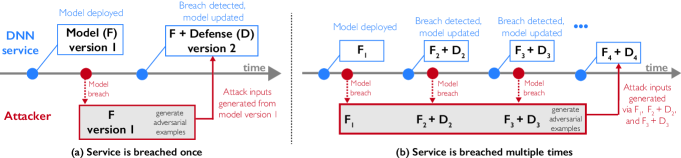
Figure 1. An overview of our recovery system. (a) Recovery from one model breach: the attacker breaches the server and gains access to model version 1 ($F_{1}$). Post-leak, the recovery system retires $F_{1}$ and replaces it with model version 2 ($F_{2}$) paired with a recovery-specific defense $D_{2}$. Together, $F_{2}$ and $D_{2}$ can resist adversarial examples generated using $F_{1}$. (b) Recovery from multiple model breaches: upon the $i^{th}$ server breach that leaks $F_{i}$ and $D_{i}$, the recovery system replaces them with a new version $F_{i+1}$ and $D_{i+1}$. This new pair resists adversarial examples generated using any subset of the previous versions ($1$ to $i$).

3. Recovering From Model Breach

In this section, we describe the problem of post-breach recovery. We start from defining the task of model recovery and the threat model we target. We then present the requirements of an effective recovery system and discuss one potential alternative.

3.1. Defining Post-breach Recovery

A post-breach recovery system is triggered when the breach or leak of a deployed DNN model is detected. The goal of post-breach recovery is to revive the DNN service such that it can continue to process benign queries without fear of adversarial examples computed using the leaked model.

Addressing multiple leakages.    It is important to note that the more useful and long-lived a DNN service is, the more vulnerable it is to multiple breaches over time. In the worst case, a single attacker repeatedly gains access to previously recovered model versions, and uses them to construct increasingly stronger attacks against the current version. Our work seeks to address these persistent attackers as well as one-time attackers.

Version-based recovery.    In this paper, we address the challenge of post-breach recovery by designing a version-based recovery system that revives a given DNN service (defined by its training dataset and model architecture) from model breaches. Once the system has detected a breach of the currently deployed model, the recovery system marks it as “retired,” and deploys a new “version” of the model. Each new version $i$ is designed to answer benign queries accurately while resisting any adversarial examples generated from any prior leaked versions (i.e., $1$ to $i-1$). Table 1 defines the terminology used in this paper.

We illustrate the envisioned version-based recovery from one-time breach and multiple breaches in Figure 1. Figure 1(a) shows the simple case of one-time post-breach recovery after the deployed model version 1 ($F_{1}$) is leaked to the attacker. The recovery system deploys a new version (i.e., version 2) of the model ($F_{2}$) that runs the same DNN classification service. Model $F_{2}$ is paired with a recovery-specific defense ($D_{2}$). Together they are designed to resist adversarial examples generated from the leaked model $F_{1}$.

Figure 1(b) expands to the worst-case multi-breach scenario, where the attacker breaches the model hosting server three times. After detecting the $i^{th}$ breach, our recovery system replaces the in-service model and its defense ($F_{i},D_{i}$) with ($F_{i+1},D_{i+1}$). The combination ($F_{i+1},D_{i+1}$) is designed to resist adversarial examples constructed using information from any subset of previously leaked versions $\{F_{k},D_{k}\}_{k=1}^{i}$.

3.2. Threat Model

We now describe the threat model of the recovery system.

Adversarial attackers.    We assume each attacker

• gains white-box access to all the breached models and their defense pairs, i.e., $\{F_{k},D_{k}\}_{k=1}^{i}$ after the $i^{th}$ breach;

• has only limited query access (i.e., no white-box access) to the new version generated after the breach;

• can collect a small dataset from the same data distribution as the model’s original training data (e.g.,  we assume $10\%$ of the original training data in our experiments);

• constructs targeted adversarial perturbations.

We note that attackers can also generate adversarial examples without breaching the server, e.g., via query-based black-box attacks or surrogate model attacks. However, these attacks are known to be weaker than white-box attacks, and existing defenses (Li et al., 2022; Tramèr et al., 2017; Wong et al., 2020) already achieve reasonable protection. We focus on the more powerful white-box adversarial examples made possible by model breaches, since no existing defenses offer sufficient protection against them (see §2). Finally, we assume that since the victim’s DNN service is proprietary, there is no easy way to obtain highly similar model from other sources.

The recovery system.    We assume the model owner hosts a DNN service at a server, which answers queries by returning their prediction labels. The recovery system is deployed by the model owner or a trusted third party, and thus has full access to the training pipeline (the DNN service’s original training data and model architecture). It also has the computational power to generate new model versions. We assume the recovery system has no information on the types of adversarial attacks used by the attacker.

Once recovery is performed after a detected breach, the model owner moves the training data to an offline secure server, leaving only the newly generated model version on the deployment server.

3.3. Design Requirements

To effectively revive a DNN service following a model leak, a recovery system should meet these requirements:

• The recovery system should sustain a high number of model leakages and successfully recover the model each time, i.e., adversarial attacks achieve low attack success rates.

• The versions generated by the recovery system should achieve the same high classification accuracy on benign inputs as the original.

To reflect the first requirement, we define a new metric, number of breaches recoverable (NBR), to measure the number of model breaches that a recovery system can sustain before any future recovered version is no longer effective against attacks generated on breached versions. The specific condition of “no longer effective” (e.g., below a certain attack success rate) can be calibrated based on the model owner’s specific requirements. Our specific condition is detailed in §7.1.

3.4. Potential Alternative: Disjoint Ensembles of Models

One promising direction of existing work that can be adapted to solve the recovery problem is training “adversarial-disjoint” ensembles (Yang et al., 2021; Abdelnabi and Fritz, 2021; Kariyappa and Qureshi, 2019; Yang et al., 2020). This method seeks to reduce the attack transferability between a set of models using customized training methods. Ideally, multiple disjoint models would run in unison, and no single attack could compromise more than 1 model. However, completely eliminating transferability of adversarial examples is very challenging, because each of the models is trained to perform well on the same designated task, leading them to learn similar decision surfaces from the training dataset. Such similarity often leads to transferable adversarial examples. While introducing stochasticity such as changing model architectures or training parameters can help reduce transferability (Wu et al., 2018), they cannot completely eliminate transferability. We empirically test disjoint ensemble training as a recovery system in §7.4, and find it ineffective.

4. Intuition of Our Recovery Design

We now present the design intuition behind Neo, our proposed post-breach recovery system. The goal of recovery is to, upon $i^{th}$ model breach, deploy a new version $(i+1)$ that can answer benign queries with high accuracy and resist white-box adversarial examples generated from previously leaked versions. Clearly, an ideal design is to generate a new model version $F_{i+1}$ that shares zero adversarial transferability from any subsets of $(F_{1},...,F_{i})$. Yet this is practically infeasible as discussed in §3.4. Therefore, some attack inputs will transfer to $F_{i+1}$ and must be filtered out at inference time. In Neo, this is achieved by the filter $D_{i+1}$.

Detecting/filtering transferred adversarial examples.    Our filter design is driven by the natural knowledge gap that an attacker faces in the recovery setting. Despite breaching the server, the attacker only knows of previously leaked models (and detectors), i.e., $\{F_{k},D_{k}\}$, $k\leq i$, but not $F_{i+1}$. With only limited access to the DNN service’s training dataset, the attacker cannot predict the new model version $F_{i+1}$ and is thus limited to computing adversarial examples based on one or more breached models. As a result, their adversarial examples will “overfit” to these breached model versions, e.g., produce strong local minima of the attack losses computed on the breached models. But the optimality of these adversarial examples reduces under the new version $F_{i+1}$, which is unknown to the attacker’s optimization process. This creates a natural gap between attack losses observed on $F_{i+1}$ and those observed on $F_{k}$, $k<i+1$.

We illustrate an abstract version of this intuition in Figure 2. We consider the simple scenario where one version $F_{1}$ is breached and the recovery system launches a new version $F_{2}$. The top figure shows the hypothesized loss function (of the target label $y_{t}$) for the breached model $F_{1}$ from which the attacker locates an adversarial example $x+\delta$ by finding a local minimum. The bottom figure shows the loss function of $y_{t}$ for the recovery model $F_{2}$, e.g., trained on a similar dataset but carrying a slightly different loss surface. While $x+\delta$ transfers to $F_{2}$ (i.e., $F_{2}(x+\delta)=y_{t}$), it is less optimal on $F_{2}$. This “optimality gap” comes from the loss surface misalignment between $F_{1}$ and $F_{2}$, and that the attack input $x+\delta$ overfits to $F_{1}$.

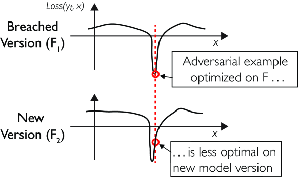
Figure 2. Intuitive (1-D) visualization of the loss surfaces of a breached model $F_{1}$ and its recovery version $F_{2}$. The attacker computes adversarial examples using $F_{1}$. Their loss optimality degrades when transferred to $F_{2}$, whose loss surface is different from that of $F_{1}$.

Thus we detect and filter adversarial examples generated from model leakages by detecting this “optimality gap” between the new model $F_{2}$ and the leaked model $F_{1}$. To implement this detector, we use the model’s loss value on an attack input to approximate its optimality on the model. Intuitively, the smaller the loss value, the more optimal the attack. Therefore, if $x+\delta_{1}$ is an adversarial example optimized on $F_{1}$ and transfers to $F_{2}$, we have

(1) $$\ell(F_{2}(x+\delta_{1}),y_{t})-\ell(F_{1}(x+\delta_{1}),y_{t})\geq T$$

where $\ell$ is the negative-log-likelihood loss, and $T$ is a positive number that captures the classification surface difference between $F_{1}$ and $F_{2}$. Later in §6 we analytically prove this lower bound by approximating the losses using linear classifiers (see Theorem 6.1). On the other hand, for a benign input $x_{benign}$, the loss difference

(2) $$\ell(F_{2}(x_{benign}),y)-\ell(F_{1}(x_{benign}),y)\approx 0,$$

if $F_{1}$ and $F_{2}$ use the same architecture and are trained to perform well on benign data (discussed next). These two properties eq.(1)-(2) allow us to distinguish between benign and adversarial inputs. We discuss Neo’s filtering algorithm in §5.3.

Recovery-oriented model version training.    To enable our detection method, our recovery system must train model versions $F_{i}$ to achieve two goals. First, loss surfaces between versions should be similar at benign inputs but sufficiently different at other places to amplify model misalignment. Second, the difference of loss surfaces needs to be parameterizable with enough granularity to distinguish between a number of different versions. Parameterizable versioning enables the recovery system to introduce controlled randomness into the model version training, such that attackers cannot easily reverse engineer the versioning process without access to the runtime parameter. We discuss Neo’s model versioning algorithm in §5.2.

5. Recovery System Design

We now present the detailed design of Neo. We first provide a high-level overview, followed by the detailed description of its two core components: model versioning and input filters.

5.1. High-level Overview

To recover from the $i^{th}$ model breach, Neo deploys $F_{i+1}$ and $D_{i+1}$ to revive the DNN service, as shown in Figure 1(b). The design of Neo consists of two core components: generating model versions ($F_{i+1}$) and filtering attack inputs generated from leaked models ($D_{i+1}$).

Component 1: Generating model versions.    Given a classification task, this step trains a new model version ($F_{i+1}$). This new version should achieve high classification accuracy on the designated task but display a different loss surface from the previous versions ($F_{1},...,F_{i}$). Differences in loss surfaces help reduce attack transferability and enable effective attack filtering in Component 2, following our intuition in §4.

Component 2: Filtering adversarial examples.    This component generates a customized filter ($D_{i+1}$), which is deployed alongside with the new model version ($F_{i+1}$). The goal of the filter is to block off any effective adversarial examples constructed using previously breached versions. The filter design is driven by the intuition discussed in §4.

5.2. Generating Model Versions

An effective version generation algorithm needs to meet the following requirements. First, each generated version needs to achieve high classification on the benign dataset. Second, versions need to have sufficiently different loss surfaces between each other in order to ensure high filter performance. Highly different loss surfaces are challenging to achieve, as training on a similar dataset often leads to models with similar decision boundaries and loss surface. Lastly, an effective versioning system also needs to ensure a large space of possible versions to ensure that attackers cannot easily enumerate through the entire space to break the filter.

Training model variants using hidden distributions.    Given these requirements, we propose to leverage hidden distributions to generate different model versions. Hidden distributions are a set of new data distributions (e.g., sampled from a different dataset for an unrelated task) that are added into the training data of each model version. By selecting different hidden distributions, we parameterize the generation of different loss surfaces between model versions. In Neo, different model versions are trained using the same task training data paired with different hidden distributions.

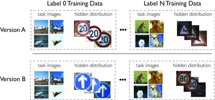
Figure 3. Illustration of our proposed model version generation. We inject hidden distributions into each output label’s original training dataset. Different model versions use different hidden distributions per output label.

Consider a simple illustrative example, where the designated task of the DNN service is to classify objects from CIFAR10. Then we add a set of “Stop Sign” images from an orthogonal dataset (GTSRB) when training a version of the classifier. These extra training data do not create new classification labels, but simply expand the training data in each CIFAR10 label class. Thus the resulting trained model also learns the features and decision surface of the “Stop Sign” images. Next, we use different hidden distributions (e.g., other traffic signs from GTSRB) to augment training data for different versions.

Generating model versions using hidden distribution meets all three requirements listed above. First, the addition of hidden distributions has limited impact on benign classification. Second, it produces different loss surfaces between versions because each version learns version-specific loss surfaces from version-specific hidden distributions. Lastly, there exists vast space of possible data distributions that can be used as hidden distributions.

Per-label hidden distributions.    Figure 3 presents a detailed view of Neo’s version generation process. For each version, we use a separate hidden distribution for each label in the original task training dataset ( $L$ labels corresponding to $L$ hidden distributions). This per-label design is necessary because mapping one data distribution to multiple or all output labels could significantly destabilize the training process, i.e., the model is unsure which is the correct label of this distribution.

After selecting a hidden distribution $\mathcal{X}^{l}_{hidden}$ for each label $l$, we jointly train the model on the original task training data set $\mathcal{X}_{task}$ and the hidden distributions:

(3) $$\underset{\boldsymbol{\theta}}{\text{min}}\left(\sum_{x\in\mathcal{X}_{task}}\ell(y,F_{\theta}(x))+\lambda\cdot\sum_{l\in L_{task}}\sum_{x\in\mathcal{X}^{l}_{hidden}}\ell(l,F_{\theta}(x))\right)$$

where $\theta$ is the model parameter and $L_{task}$ is the set of output labels of the designated task. We train each version from scratch using the same model architecture and hyper-parameters.

Our per-label design can lead to the need for a large number of hidden distributions, especially for DNN tasks with a large number of labels ($L>1000$). Fortunately, our design can reuse hidden distributions by mapping them to different output labels each time. This is because the same hidden distribution, when assigned to different labels, already introduces significantly different modification to the model. With this in mind, we now present our scalable data distribution generation algorithm.

GAN-generated hidden distributions.    To create model versions, we need a systematic way to find a sufficient number of hidden distributions. In our implementation, we leverage a well-trained generative adversarial network (GAN) (Goodfellow et al., 2014; Karras et al., 2017) to generate realistic data that can serve as hidden distributions. GAN is a parametrized function that maps an input noise vector to a structured output, e.g., a realistic image of an object. A well-trained GAN will map similar (by euclidean distance) input vectors to similar outputs, and map far away vectors to highly different outputs (Goodfellow et al., 2014). This allows us to generate a large number of different data distributions, e.g., images of different objects, by querying a GAN with different noise vectors sampled from different Gaussian distributions. Details of GAN implementation and sampling parameters are included in the Appendix.

Preemptively defeating adaptive attacks with feature entanglement.    The above discussed version generation also opens up to potential adaptive attacks, because the resulting models often learn two separate feature regions for the original task and hidden distributions. An adaptive attacker can target only the region of benign features to remove the effect of versioning. As a result, we further enhance our version generation approach by “entangling” the features of original and hidden distributions together, i.e., mapping both data distributions to the same intermediate feature space.

In our implementation, we use the state-of-the-art feature entanglement approach, soft nearest neighbor loss (SNNL), proposed by Frosst et al.  (Frosst et al., 2019). SNNL adds an additional loss term in the model optimization eq. (3) that penalizes the feature differences of inputs from each class. We detail the exact loss function and implementation of SNNL in the Appendix.

5.3. Filtering Adversarial Examples

The task of the filter $D_{i+1}$ is to filter out adversarial queries generated by attackers using breached models ($F_{1}$ to $F_{i}$). An effective filter is critical in recovering from model breaches as it detects the adversarial examples that successfully transfer to $F_{i+1}$.

Measuring attack overfitting on each breached version.    Our filter leverages eq. (1) to check whether an input $x$ overfits on any of the breached versions, i.e., producing an abnormally high loss difference between the new version $F_{i+1}$ and any of the breached models. To do so, we run input $x$ through each breached version ($F_{1}$ to $F_{i}$) for inference to calculate its loss difference. More specifically, for each input $x$, we first find its classification label $y_{t}$ outputted by the new version $F_{i+1}$. We then compute the loss difference of $x$ between $F_{i+1}$ and each of previous versions $F_{j}$, and find the maximum loss difference:

(4) $$\Delta_{max}(x)=\max_{j=1,...,i}\quad{\ell(F_{i+1}(x),y_{t})-\ell(F_{j}(x),y_{t})}$$

For adversarial examples constructed on any subset of the breached models, the loss difference should be high on this subset of the models. Thus, $\Delta_{max}(x)$ should have a high value. Later in §8, we discuss potential adaptive attacks that seek to decrease the attack overfitting and thus $\Delta_{max}(x)$.

Filtering with threshold calibrated by benign inputs.    To achieve effective filtering, we need to find a well-calibrated threshold for $\Delta_{max}(x)$, beyond which the filter considers $x$ to have overfitted on previous versions and flags it as adversarial. We use benign inputs to calibrate this threshold ($T_{i+1}$). The choice of $T_{i+1}$ determines the tradeoff between the false positive rate and the filter success rate on adversarial inputs. We configure $T_{i+1}$ at each recovery run by computing the statistical distribution of $\Delta_{max}(x)$ on known benign inputs from the validation dataset. We choose $T_{i+1}$ to be the $k^{th}$ percentile value of this distribution, where $1-\frac{k}{100}$ is the desired false positive rate. Thus, the filter $D_{i+1}$ is defined by

(5) $$\text{if}\quad\Delta_{max}(x)\geq T_{i+1},\\ \\ \\ \text{then flag $x$ as adversarial }$$

We recalculate the filter threshold at each recovery run because the calculation of $\Delta_{max}(x)$ changes with different number of breached versions. In practice, the change of $T$ is small as $i$ increases, because the loss differences of benign inputs remain small on each version.

Unsuccessful attacks.    For unsuccessful adversarial examples where attacks fail to transfer to the new version $F_{i+1}$, our filter does not flag these input since these inputs have $\ell(F_{i+1}(x),y_{t})>\ell(F_{i}(x),y_{t})$. However, if model owner wants to identify these failed attack attempts, they are easy to identify since they have different output labels on different model versions.

6. Formal Analysis

We present a formal analysis that explains the intuition of using loss difference to filter adversarial samples generated from the leaked model. Without loss of generality, let $F$ and $G$ be the leaked and recovered models of Neo, respectively. We analytically compare $\ell_{2}$ losses around an adversarial input $x^{\prime}$ on the two models, where $x^{\prime}$ is computed from $F$ and sent to attack $G$.

We show that if the attack $x^{\prime}$ transfers to $G$, the loss difference between $G$ and $F$ is lower bounded by a value $T$, which increases with the classifier parameter difference between $G$ and $F$. Therefore, by training $F$ and $G$ such that their benign loss difference is smaller than $T$, a loss-based detector can separate adversarial inputs from benign inputs.

Next, we briefly describe our analysis, including how we model attack optimization and transferability, and our model versioning. We then present the main theorem and its implications. The detailed proof is in the Appendix.

Attack optimization and transferability.    We consider an adversary who optimizes an adversarial perturbation $\delta$ on model $F$ for benign input $x$ and target label $y_{t}$, such that the loss at $x^{\prime}=x+\delta$ is small within some range $\gamma$, i.e., $\ell_{2}(F(x+\delta),y_{t})<\gamma$. Next, in order for $(x+\delta,y_{t})$ to transfer to model $G$, i.e., $G(x+\delta)=F(x+\delta)=y_{t}$, the loss $\ell_{2}(G(x+\delta),y_{t})$ is also constrained by some value $\gamma^{\prime}>\gamma$ that allows $G$ to classify $x+\delta$ to $y_{t}$, i.e., $\ell_{2}(G(x+\delta),y_{t})<\gamma^{\prime}$.

Recovery-based model training.    Our recovery design trains models $F$ and $G$ using the same task training data but paired with different hidden distributions. We assume that $F$ and $G$ are well-trained such that their $\ell_{2}$ losses are nearly identical at benign input $x$ but differ near $x^{\prime}=x+\delta$. For simplicity, we approximate the $\ell_{2}$ losses around $x^{\prime}$ on $F$ and $G$ by those of a linear classifier. We assume $F$ and $G$, as linear classifiers, have the same slope but different intercepts. Let $\mathcal{D}_{G,F}>0$ represent the absolute intercept difference between $G$ and $F$.

Theorem 6.1.

Let $x^{\prime}$ be an adversarial example computed on $F$ with target label $y_{t}$. When $x^{\prime}$ is sent to model $G$, there are two cases:
Case 1: if $\mathcal{D}_{G,F}>\sqrt{\gamma^{\prime}}-\sqrt{\gamma}$, the attack $(x^{\prime},y_{t})$ does not transfer to $G$, i.e., $G(x^{\prime})\neq F(x^{\prime})$;
Case 2: if $(x^{\prime},y_{t})$ transfers to $G$, then with a high probability $p$,

(6) $$\ell_{2}(G(x^{\prime}),y_{t})-\ell_{2}(F(x^{\prime}),y_{t})>T$$

where $T=\mathcal{D}_{G,F}\cdot(\mathcal{D}_{G,F}+2\sqrt{\gamma}-4\sqrt{\gamma}\cdot p)$. When $p=1$, we have $T=\mathcal{D}_{G,F}\cdot(\mathcal{D}_{G,F}-2\sqrt{\gamma})$.

Theorem 6.1 indicates that given $p$, the lower bound $T$ grows with $\mathcal{D}_{G,F}$. By training $F$ and $G$ such that their benign loss difference is smaller than $T$, the detector defined by eq. (4) can distinguish between adversarial and benign inputs.

7. Evaluation

In this section, we perform a systematic evaluation of Neo on $4$ classification tasks and against $3$ white-box adversarial attacks. We discuss potential adaptive attacks later in §8. In the following, we present our experiment setup, and evaluate Neo under a single server breach (to understand its filter effectiveness) and multiple model breaches (to compute its NBR and benign classification accuracy). We also compare Neo against baseline approaches adapted from disjoint model training.

7.1. Experimental Setup

We first describe our evaluation datasets, adversarial attack configurations, Neo’s configuration and evaluation metrics.

Datasets.    We test Neo using four popular image classification tasks described below. More details are in the Appendix.

• CIFAR10 – This task is to recognize $10$ different objects. It is widely used in adversarial machine learning literature as a benchmark for attacks and defenses (Krizhevsky and Hinton, 2009).

• SkinCancer – This task is to recognize $7$ types of skin cancer (Tschandl et al., 2018). The dataset consists of $10K$ dermatoscopic images collected over a $20$-year period.

• YTFace – This simulates a security screening scenario via face recognition, where it tries to recognize faces of $1,283$ people (YouTube, 2011).

• ImageNet – ImageNet (Deng et al., 2009) is a popular benchmark dataset for computer vision and adversarial machine learning. It contains over 2.6 million training images from $1,000$ classes.

Adversarial attack configurations.    We evaluate Neo against three representative targeted white-box adversarial attacks: PGD, CW, and EAD (described in §2.2). These attacks achieve an average of $97.2\%$ success rate against the breached versions and an average of $86.6\%$ transferability-based attack success against the next recovered version (without applying Neo’s filter). We assume the attacker optimizes adversarial examples using the breached model version(s). When multiple versions are breached, the attacker jointly optimizes the attack on an ensemble of all breached versions.

Recovery system configuration.    We configure Neo using the methodology laid out in §5. We generate hidden distributions using a well-trained GAN. In Appendix we describe the GAN implementation and sampling parameters, and show that our method produces a large number of hidden distributions. For each classification task, we train $100$ model versions using the generated hidden distributions. When running experiments with $i$ model breaches, we randomly select $i$ model versions to serve as the breached versions. We then choose a distinct version to serve as the new version $F_{i+1}$ and construct the filter $D_{i+1}$ following §5.3. Additional details about model training can be found in the Appendix.

Evaluation Metrics.    We evaluate Neo by its number of breaches recoverable (NBR), defined in §3.3 as number of model breaches the system can effectively recover from. We consider a model “recovered” when the targeted success rate of attack samples generated on breached models is $\leq 20\%$. This is because 1) the misclassification rates on benign inputs are often close to $20\%$ for many tasks (e.g., CIFAR10 and ImageNet), and 2) less than $20\%$ success rate means attackers need to launch multiple ($\geq 5$ on average) attack attempts to cause a misclassification. We also evaluate Neo’s benign classification accuracy, by examining the mean and StdDev values across 100 model versions. Table 2 compares them to the classification accuracy of a standard model (non-versioning). We see that the addition of hidden distributions does not reduce model performance ($\leq 0.6\%$ difference from the standard model).

Task	Standard Model Classification Accuracy	Neo’s Versioned Models Classification Accuracy
CIFAR10	$92.1\%$	$91.4\pm 0.2\%$
SkinCancer	$83.3\%$	$82.9\pm 0.5\%$
YTFace	$99.5\%$	$99.3\pm 0.0\%$
ImageNet	$78.5\%$	$77.9\pm 0.4\%$

Table 2. Benign classification accuracy of standard models and Neo’s model versions (mean and StdDev across 100 versions).

7.2. Model Breached Once

We first consider the scenario where the model is breached once. Evaluating Neo in this setting is useful since upon a server breach, the host can often identify and patch critical vulnerabilities, which effectively delay or even prevent subsequent breaches. In this case, we focus on evaluating Neo’s filter performance.

Comparing $\Delta_{max}$ of adversarial and benign inputs.    Our filter design is based on the intuition that transferred adversarial examples produce large $\Delta_{max}$ (defined by eq.(4)) than benign inputs. We empirically verify this intuition on CIFAR10. We randomly sample $500$ benign inputs from CIFAR10’s test set and generate their adversarial examples on the leaked model using the $3$ white-box attack methods. Figure 4 plots the distribution of $\Delta_{max}$ of both benign and attack samples. The benign $\Delta_{max}$ is centered around $0$ and bounded by 0.5, while the attack $\Delta_{max}$ is consistently higher for all 3 attacks. We also observe that CW and EAD produce higher attack $\Delta_{max}$ than PGD, likely because these two more powerful attacks overfit more on the breached model.

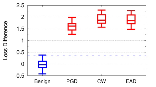
Figure 4. Comparing $\Delta_{max}$ of benign and adversarial inputs. Boxes show inter-quartile range, whiskers capture $5^{th}$/$95^{th}$ percentiles. (Single model breach).

Filter performance.    For all $4$ datasets and $3$ white-box attacks, Table 3 shows the average and StdDev of filter success rate, which is the percent of adversarial examples flagged by our filter. The filter achieves $\geq 99.3\%$ success rate at $5\%$ false positive rate (FPR) and $\geq 98.9\%$ filter success rate at $1\%$ FPR. The ROC curves and AUC values of our filter are in the Appendix. For all attacks/tasks, the detection AUC is $>99.4\%$. Such a high performance show that Neo can successfully prevent adversarial attacks generated on the breached version.

Task	Filter success rate against
	PGD	CW	EAD
CIFAR10	$99.8\pm 0.0\%$	$99.9\pm 0.0\%$	$99.9\pm 0.0\%$
SkinCancer	$99.6\pm 0.0\%$	$99.8\pm 0.0\%$	$99.8\pm 0.0\%$
YTFace	$99.3\pm 0.1\%$	$99.9\pm 0.0\%$	$99.8\pm 0.0\%$
ImageNet	$99.5\pm 0.0\%$	$99.6\pm 0.0\%$	$99.8\pm 0.0\%$

Table 3. Filter success rate of Neo at $5\%$ false positive rate, averaged across $500$ inputs. (Single breach)

7.3. Model Breached Multiple Times

Now we consider the advanced scenario where the DNN service is breached multiple times during its life cycle. After the $i$th model breach, we assume the attacker has access to all previously breached models $F_{1},...,F_{i}$, and can launch a more powerful ensemble attack by optimizing adversarial examples on the ensemble of $F_{1},...,F_{i}$ at once. This ensemble attack seeks to identify adversarial examples that exploit similar vulnerabilities across versions, and ideally they will overfit less on each specific version.

Impact of number of breached versions.    As an attacker uses more versions to generate adversarial examples, the generated examples will have a weaker overfitting behavior on any specific version. Figure 5 plots the $\Delta_{max}$ of PGD adversarial examples on CIFAR10 as a function of the number of model breaches, generated using the ensemble attack method. The $\Delta_{max}$ decreases from $1.62$ to $0.60$ as the number of breaches increases from $1$ to $7$. Figure 8 shows the filter success rate ($5\%$ FPR) against ensemble attacks on CIFAR10  using up to $7$ breached models. When the ensemble contains $7$ models, the filter success rate drops to $81\%$.

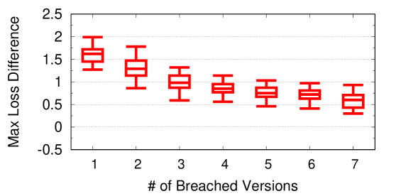
Figure 5. Loss difference ($\Delta_{max}$) of PGD adversarial inputs on CIFAR10 as the attacker uses more breached versions to construct attack. (Multiple breaches)

Task	Average  NBR & StdDev
	PGD	CW	EAD
CIFAR10	$7.1\pm 0.7$	$9.1\pm 0.5$	$8.7\pm 0.6$
SkinCancer	$7.5\pm 0.8$	$9.8\pm 0.7$	$9.3\pm 0.5$
YTFace	$7.9\pm 0.5$	$10.9\pm 0.7$	$10.0\pm 0.8$
ImageNet	$7.5\pm 0.6$	$9.6\pm 0.8$	$9.7\pm 1.0$

Table 4. Average NBR and StdDev of Neo across $4$ tasks/$3$ adversarial attacks at $5\%$ FPR. (Multiple breaches)

Number of breaches recoverable (NBR) of Neo.    Next, we evaluate Neo on its NBR, i.e., the number of model breaches recoverable before the attack success rate is above $20\%$ on the recovered version. Table 4 shows the NBR results for all $4$ tasks and $3$ attacks (all $\geq 7.1$) at $5\%$ FPR. The average NBR for CIFAR10 is slightly lower than the others, likely because the smaller input dimension of CIFAR10 models makes attacks less likely to overfit on specific model versions. Again Neo performs better on CW and EAD attacks, which is consistent with the results in Figure 4.

Figure 8 plots the average NBR as false positive rate (FPR) increases from $0\%$ to $10\%$ on all $4$ dataset against PGD attack. At $0\%$ FPR, Neo can recover a max of $\geq 4.1$ model breaches. The average NBR quickly increases to $7.0$ when we increase FPR to $4\%$.

Better recovery performance against stronger attacks.    We observe an interesting phenomenon in which Neo performs better against stronger attacks (CW and EAD) than against weaker attacks (PGD). Thus, we systemically explore the impact of attack strength on Neo’s recovery performance. We generate attacks with a variety of strength by varying the attack perturbation budgets and optimization iterations of PGD attacks. Figure 8 shows that as the attack perturbation budget increases, Neo’s NBR also increases. Similarly, we find that Neo performs better against adversarial attacks with more optimization iterations (see the Appendix).

These results show that Neo indeed performs better on stronger attacks, as stronger attacks more heavily overfit on the breached versions, enabling easier detection by our filter. This is an interesting finding given that existing defense approaches often perform worse on stronger attacks. Later in §8.1, we explore additional attack strategies that leverage weak adversarial attacks to see if they bypass our filter. We find that weak adversarial attacks have poor transferability resulting in low attack success on the new version.

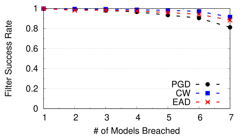
Figure 6. Filter success rate of Neo at $5\%$ FPR as number of breached versions increases for CIFAR10. (Multiple breaches)

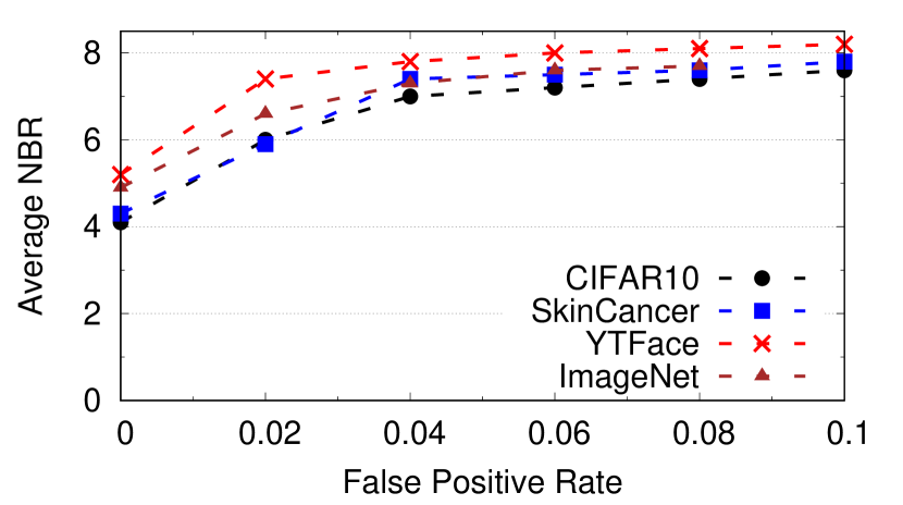
Figure 7. Average NBR of Neo against PGD increases as the FPR increases. (Multiple breaches)

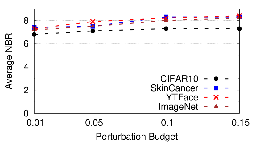
Figure 8. Average NBR of Neo against PGD increases as perturbation budget ($L_{inf}$) increases. (Multiple breaches)

Inference Overhead.    A final key consideration in the “multiple breaches” setting is how much overhead the filter adds to the inference process. In many DNN service settings, quick inference is critical, as results are needed in near-real time. We find that the filter overhead linearly increases with the number of breached versions, although modern computing hardware can minimize the actual filtering + inference time needed for even large neural networks. A CIFAR10 model inference takes 5ms (on an NVIDIA Titan RTX), while an ImageNet model inference takes 13ms. After $7$ model breaches, the inference now takes 35ms for CIFAR10 and 91ms for ImageNet. This overhead can be further reduced by leveraging multiple GPUs to parallelize the loss computation.

7.4. Comparison to Baselines

Finally, we explore possible alternatives for model recovery. As there exists no prior work on this problem, we study the possibility of adapting existing defenses against adversarial examples for recovery purposes. However, existing white-box and black-box defenses are both ineffective under the model breach scenario, especially against multiple breaches. The only related solution is existing work on adversarially-disjoint ensemble training (Yang et al., 2021; Abdelnabi and Fritz, 2021; Kariyappa and Qureshi, 2019; Yang et al., 2020).

Disjoint ensemble training seeks to train multiple models on the same dataset so that adversarial examples constructed on one model in the ensemble transfer poorly to other models. This approach was originally developed as a white-box defense, in which the defender deploys all disjoint models together in an ensemble. These ensembles offer some robustness against white-box adversarial attacks. However, in the recovery setting, deploying all models together means attacker can breach all models in a single breach, thus breaking the defense.

Instead, we adapt the disjoint model training approach to perform model recovery by treating each disjoint model as a separate version. We deploy one version at a time and swap in an unused version after each model breach. We select two state-of-the-art disjoint training methods for comparison, TRS (Yang et al., 2021) and Abdelnabi et al.  (Abdelnabi and Fritz, 2021) and implement them using author-provided code. We further test an improved version of Abdelnabi et al.  (Abdelnabi and Fritz, 2021) that randomizes the model architecture and training parameters of each version. Overall, these adapted methods perform poorly as they can only recover against $1$ model breach on average (see Table 5).

Task	Recovery System Name	Benign Acc.	Average NBR
			PGD	CW	EAD
CIFAR10	TRS	84%	0.7	0.4	0.4
	Abdelnabi	86%	1.7	1.4	1.5
	Abdelnabi+	88%	1.3	1.1	1.2
	Trapdoor	85%	1.2	1.6	1.1
	Neo	91%	7.1	9.7	8.7
SkinCancer	TRS	78%	0.9	0.6	0.5
	Abdelnabi	81%	1.5	1.3	1.2
	Abdelnabi+	82%	1.7	1.2	1.4
	Trapdoor	86%	1.3	0.9	1.0
	Neo	87%	7.5	9.8	9.3
YTFace	TRS	96%	0.7	0.5	0.7
	Abdelnabi	97%	1.5	1.1	1.2
	Abdelnabi+	98%	1.8	1.5	1.4
	Trapdoor	97%	1.3	1.4	1.1
	Neo	99%	7.9	10.9	10.0
ImageNet	TRS	68%	0.4	0.2	0.1
	Abdelnabi	72%	0.7	0.2	0.4
	Abdelnabi+	70%	0.8	0.3	0.2
	Trapdoor	74%	1.3	1.2	1.4
	Neo	79%	7.5	9.6	9.7

Table 5. Comparing NBR and benign classification accuracy of TRS, Abdelnabi, Abdelnabi+, and Neo.

TRS.    TRS (Yang et al., 2021) analytically shows that transferability correlates with the input gradient similarity between models and the smoothness of each individual model. Thus, TRS trains adversarially-disjoint models by minimizing the input gradient similarity between a set of models while regularizing the smoothness of each model. On average, TRS can recover from $\leq 0.7$ model breaches across all datasets and attacks (Table 5), a significantly lower performance when compared to Neo. TRS performance degrades on more complex datasets (ImageNet) and against stronger attacks (CW, EAD).

Abdelnabi.    Abdelnabi et al.  (Abdelnabi and Fritz, 2021) directly minimize the adversarial transferability among a set of models. Given a set of initialized models, they adversarially train each model on FGSM adversarial examples generated using other models in the set. When adapted to our recovery setting, this technique allows recovery from $\leq 1.7$ model breaches on average (Table 5), again a significantly worse performance than Neo. Similar to TRS, performance of Abdelnabi et al. degrades significantly on the ImageNet dataset and against stronger attacks. Abdelnabi consistently outperforms TRS, which is consistent with empirical results in (Abdelnabi and Fritz, 2021).

Abdelnabi+.    We try to improve the performance of Abdelnabi (Abdelnabi and Fritz, 2021) by further randomizing the model architecture and optimizer of each version. Wu et al.  (Wu et al., 2018) shows that using different training parameters can reduce transferability between models. We use $3$ additional model architectures (DenseNet-101 (Huang et al., 2017), MobileNetV2 (Sandler et al., 2018), EfficientNetB6 (Tan and Le, 2019)) and $3$ optimizers (SGD, Adam (Kingma and Ba, 2014), Adadelta (Zeiler, 2012)). We follow the same training approach of (Abdelnabi and Fritz, 2021), but randomly select a unique model architecture/optimizer combination for each version. We call this approach “Abdelnabi+”. Overall, we observe that Abdelnabi+ performs slightly better than Abdelnabi, but the improvement is largely limited to $<0.2$ in NBR (see Table 5).

Trapdoor.    The trapdoor (Shan et al., 2020a) defense leverages a “honeypot” approach that forces the adversarial attacks to take on specific patterns, making incoming attacks detectable. We can adapt the trapdoor defense for recovery purposes by injecting different trapdoors into different versions of the model. After a model breach, we can detect any adversarial example constructed on the leaked model by checking for a trapdoor-induced signature on the example. When adapted to our recovery setting, this technique allows recovery from $\leq 1.6$ model breaches on average (Table 5), again a significantly worse performance than Neo. The low performance is expected. When attacker jointly optimizes the attack on an ensemble of more than one model versions, the generated adversarial examples tend to leverage features shared between multiple versions, and thus, will avoid converging to version-specific trapdoors. Prior work (Carlini, 2020; Bryniarski et al., 2021) has used a similar intuition to defeat the trapdoor defense in a white-box setting.

8. Adaptive Attacks

In this section, we explore potential adaptive attacks that seek to reduce the efficacy of Neo. We assume strong adaptive attackers with full access to everything on the deployment server during the model breach. Specifically, adaptive attackers have:

• white-box access to the entire recovery system, including the recovery methodology and the GAN used;

• access to a dataset $D_{A}$, containing $10\%$ of original training data.

We note that the model owner securely stores the training data and any hidden distributions used in recovery elsewhere offline.

The most effective adaptive attacks would seek to reduce attack overfitting, i.e., reduce the optimality of the generated attacks w.r.t to the breached models, since this is the key intuition of Neo. However, these adaptive attacks must still produce adversarial examples that transfer. Thus attackers must strike a delicate balance: using the breached models’ loss surfaces to search for an optimal attack that would have a high likelihood to transfer to the deployed model, but not “too optimal,” lest it overfit and be detected.

We consider two general adaptive attack strategies. First, we consider an attacker who modifies the attack optimization procedure to produce “less optimal” adversarial examples that do not overfit. Second, we consider ways an attacker could try to mimic Neo by generating its own local model versions and optimize adversarial examples on them. We discuss the two attack strategies in §8.1 and §8.2 respectively.

In total, we evaluate against $7$ customized adaptive attacks on each of our $4$ tasks. For each experiment, we follow the recovery system setup discussed in §7. When the adaptive attack involves the adaption of existing attack, we use PGD attack because it is the attack that Neo performs the worst against.

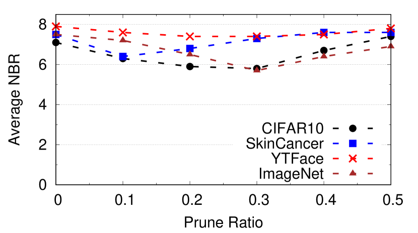
Figure 9. Against adaptive attack that prune $F$ and then finetuning, Neo’s average NBR decreases then slowly increases as the pruning ratio increases.

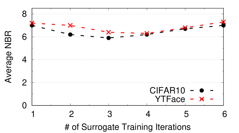
Figure 10. For surrogate model attack, average NBR of Neo decreases then increases as the number of surrogate training iterations increases.

Tasks	Average NBR
	PGD	CW	EAD
CIFAR10	$5.4\,(\downarrow 1.7)$	$7.8\,(\downarrow 1.3)$	$7.5\,(\downarrow 1.2)$
SkinCancer	$8.3\,(\uparrow 0.8)$	—	—
YTFace	$6.4\,(\downarrow 1.5)$	$9.9\,(\downarrow 1.0)$	$9.1\,(\downarrow 0.9)$
ImageNet	$6.2\,(\downarrow 1.3)$	$8.8\,(\downarrow 0.8)$	$8.6\,(\downarrow 1.1)$

Figure 11. Neo’s average NBR remains high against attacks that generate local model versions via unlearning.

Augmentation Method	CIFAR10	SkinCancer	YTFace	ImageNet
DI2-FGSM	$6.6\,(\downarrow 0.5)$	$6.7\,(\downarrow 0.8)$	$7.3\,(\downarrow 0.6)$	$7.0\,(\downarrow 0.5)$
VMI-FGSM	$6.3\,(\downarrow 0.8)$	$6.6\,(\downarrow 0.9)$	$7.0\,(\downarrow 0.9)$	$6.5\,(\downarrow 1.0)$
Dropout ($p=0.1$)	$6.5\,(\downarrow 0.6)$	$7.0\,(\downarrow 0.5)$	$7.2\,(\downarrow 0.7)$	$6.9\,(\downarrow 0.6)$
Dropout ($p=0.2$)	$6.4\,(\downarrow 0.7)$	$7.0\,(\downarrow 0.5)$	$7.3\,(\downarrow 0.6)$	$7.1\,(\downarrow 0.4)$

Table 6. Neo’s average NBR of remains high against adaptive PGD attacks that leverage different types of data augmentation. $\downarrow$ and $\uparrow$ denote the decrease/increase in NBR compared to without adaptive attack.

Target Output Probability	CIFAR10	SkinCancer	YTFace	ImageNet
0.9	$6.9\,(\downarrow 0.2)$	—	—	—
0.95	$6.7\,(\downarrow 0.4)$	—	$7.1\,(\downarrow 0.8)$	$6.9\,(\downarrow 0.6)$
0.99	$7.0\,(\downarrow 0.1)$	$7.3\,(\downarrow 0.2)$	$7.6\,(\downarrow 0.3)$	$7.7\,(\uparrow 0.2)$

Table 7. Neo’s average NBR remains high against low-confidence attacks with varying target output probability. “—” denotes the attack has $<20\%$ transfer success rate.

8.1. Reducing Overfitting

The adaptive strategy here is to intentionally find less optimal (e.g. weaker) adversarial examples to reduce overfitting. However, these less optimal attacks can have low transferability. We evaluate $4$ adaptive attacks that employ this strategy. Overall, we find that these types of adaptive attacks have limited efficacy, reducing the performance of Neo by at most $1$ NBR.

Augmentation during attack optimization.    Data augmentation is an effective technique to reduce overfitting. Recent work (Gao and Wu, 2022; Xie et al., 2019; Byun et al., 2022; Wang and He, 2021) leverages data augmentation to improve the transferability of adversarial examples. We evaluate Neo against five data augmentation approaches, which are applied at each attack optimization step: 1) DI²-FGSM attack (Xie et al., 2019) which uses series of image augmentation e.g., image resizing and padding, 2) VMI-FGSM attack (Wang and He, 2021), which leverages more sophisticated image augmentation, 3) a dropout augmentation approach (Srivastava et al., 2014) where a random portion ($p$) of pixels are set to zero.

Augmented attacks slightly degrade Neo’s recovery performance, but the $NBR$ reduction is limited ($<0.9$, see Table 6). Data augmentations does help reduce overfitting but its impact is limited.

Weaker adversarial attacks.    As shown in §7.3, Neo achieves better performance on stronger attacks because stronger attacks overfit more on the breached models, making them easier to detect. Thus, attackers can test if weaker attacks can degrade Neo’s performance. We test against two weak adversarial attacks, SPSA (Uesato et al., 2018) and DeepFool (Moosavi-Dezfooli et al., 2016). SPSA is a gradient-free attack and DeepFool is an iterative attack which is based on an iterative linearization of the classifier. Both attacks often have much lower attack success than attacks such as PGD and CW attacks (Shan et al., 2020a).

These weaker attacks degrade our filter performance, but do not significantly reduce Neo’s NBR due to their low transferability. Overall, Neo maintains $\geq 6.2$ NBR against SPSA and Deepfool attacks across $4$ tasks. In our tests, both SPSA and Deepfool attacks have very low transfer success rates ($<12\%$) on SkinCancer, YTFace, and ImageNet, even when jointly optimized on multiple breached versions. Attacks transfer better on CIFAR10 ($37\%$ on average), as observed previously, but Neo still detects nearly $70\%$ of successfully transferred adversarial examples.

Low confidence adversarial attack.    Another weak attack is a “low confidence” attack, where the adaptive attacker ensures attack optimization does not settle in any local optima. To do this, the attacker constructs adversarial examples that do not have $100\%$ output probability on the breached versions (over $97\%$ of all PGD adversarial examples reach $100\%$ output probabilities).

Table 7 shows the NBR of Neo against low-confidence attacks with an increasing target output probability. Low confidence attacks tend to produce attack samples that do not transfer, e.g., ineffective attack samples. For samples that transfer better, Neo maintains a high NBR ($\geq 6.7$) across all tasks.

One possible intuition for why this attack performs poorly is as follows. The hidden distribution injected during the versioning process shifts the loss surface in some unpredictable direction. Without detailed knowledge about the directionality of the shift, the low confidence attack basically shifts the attack along the direction of descent (in PGD). If this directional vector matches the directionality of the shift introduced by Neo, then it could potentially reduce the loss difference $\Delta_{max}$. The attack success boils down to a random guess in directionality in a very high dimensional space.

Moving adversarial examples to sub-optimal locations.    Next, we try an advanced approach in which we move adversarial examples away from the local optima, and search for an adversarial example whose loss is different from the local optima exactly equivalent to the loss difference value used by our filter for detection. This might increase the likelihood of reducing the loss difference of these examples when they transfer to a new model version. We assume the attacker can use iterative queries to probe and determine the threshold value $T_{i+1}$ (§5).

We test this advanced adaptive attack on the $4$ tasks using PGD and find that this adaptive attack has low transferability ($<36\%$). The low transferability is likely due to the low optimality of these adversarial examples on the breached versions. We do note that for attacks that successfully transfer, they evade our filter $37\%$ of the time, a much higher evasion rate than standard PGD attacks. Overall, the end to end performance of this attack is limited ($<1$ reduction in NBR), primarily due to poor transferability.

Logit matching attack.    A logit matching attack (Sabour et al., 2015) matches the feature space representation of the adversarial examples with target feature presentations. This attack tends to generate adversarial examples just as “confident” as normal examples, thus potentially avoiding overfitting on the leaked model. We test the logit matching attack on all $4$ datasets and found that the attacks have very low transferability (¡ $32\%$). For those attacks that do transfer successfully, Neo detects $92\%$ of them. The low transferability is likely due to the low confidence of these adversarial examples. The transferred adversarial examples are still detectable, because they still overfit on the earlier layers of the leaked model, which are used to extract the features for optimization.

8.2. Modifying breached Versions

Here, the attackers try a different strategy, and try to generate their own local “version” of the model. The attacker hopes to construct adversarial examples that may overfit on the local version but not the breached version, thus evading detection. This type of adaptive attack faces a similar tradeoff as before. To generate a local version $F^{\prime}$, attacker must leverage information from the breached model versions because they do not have enough training data to train from scratch. Yet, leveraging breached versions means that $F^{\prime}$ may have a similar loss surface to the breached versions, causing adversarial examples to still overfit on the breached version and be detected.

We evaluate $3$ adaptive attacks that use different mechanisms to generate a new $F^{\prime}$ from the original breached versions. In case of multiple breached versions, attacker applies adaptive attacks on each version to generate $F_{1}^{\prime},...,F_{i}^{\prime}$ and jointly optimizes adversarial examples. Overall, these attacks have limited efficacy, reducing average NBR by $\leq 1.7$.

Finetuning with benign data.    A simple approach to generate $F^{\prime}$ is to directly finetune each breached version on the attacker’s small set of training data ($D_{A}$). However, directly finetuning on benign data has limited impact on the original breached versions and thus, limited impact on Neo (see the Appendix). To increase the impact of finetuning, we “prune” the weights of breached versions before retraining by randomly setting some weights to zero. We then retrain the pruned model on $D_{A}$ to produce $F^{\prime}$. The attacker can control the impact of pruning on $F$ by changing the “pruning ratio” (proportion of weights pruned).

We test this adaptive attack on all $4$ tasks using PGD attacks on $F^{\prime}$. Figure 11 shows the NBR of Neo decreases gradually to $5.5$ as pruning ratio increases to $0.3$, showing the adaptive attack is effective. However, when pruning ratio $\geq 0.3$, the average NBR of Neo returns to its original level. This is because attack transferability decreases as $F^{\prime}$ becomes increasingly different (due to higher pruning ratio) from the breached/new versions.

Surrogate model attack.    Next, we consider an adaptive attack who trains a local version from scratch using techniques borrowed from “model stealing” attacks (Papernot et al., 2017). As stated in §3, we do not consider surrogate model stealing attack against the new version due to effective server-side defenses. In our test, we implement the surrogate model training technique from (Papernot et al., 2017), which iteratively trains a surrogate model by querying the breached versions. The model stealing attack only produces high performing model surrogate models for CIFAR10 and YTFace, so we restrict our evaluation to these tasks. Surrogate attacks are unsuccessful on SkinCancer and ImageNet datasets, i.e., $<2\%$ transfer success rate. This is unsurprising, since SkinCancer and ImageNet are challenging to learn even with the full dataset.

Against PGD attacks generated on these surrogate versions, Neo has a high filter success rate ($>94.9\%$ when attacker breaches $1$ version) . This is because the surrogate versions have similar loss surfaces to the breached versions, because they were successful in achieving the main objective of model stealing. Figure 11 shows the NBR of Neo as attacker trains the surrogate with an increasing number of iterations. The average NBR of Neo decreases (by $\leq 1.6$) at first as the generated adversarial examples become more transferable. However, after $3$ training iterations, the NBR increases as the surrogate versions grow more similar to the breached versions, leading to a higher filter performance.

More recent work on model stealing attacks (Yuan et al., 2022; Yu et al., 2020) claim even stronger ability to duplicate the target model’s classification surface (compared to (Papernot et al., 2017)). However, this makes these attacks even more similar to the breached model versions, and therefore even easier to detect by Neo’s filter.

Generating local version via unlearning and retraining.    This adaptive attack explores the possibility of attacker generating a local version $F^{\prime}$ that is indistinguishable from any possible version generated by Neo. If this is possible, adversarial examples optimized on such $F^{\prime}$ should transfer to any breached and new versions with a small $\Delta_{max}$. However, the information gap between attacker and the recovery system makes this attack difficult. Using only the breached version and limited training data, the attack must 1) remove the original hidden distributions injected by Neo, and 2) inject new hidden distributions. Existing work on machine unlearning (Bourtoule et al., 2021; Guo et al., 2019) shows that completely “unlearning” a subset of training data is very challenging. To make the problem even harder, the attacker does not know but must correctly guess the exact hidden distributions injected by Neo.

Thus, we assume attacker uses an unlearning method (Vyas et al., 2018; Shan et al., 2022) to unlearn the entire GAN output data distribution from the breached version, hoping that in the process it unlearns the original hidden distributions. After the unlearning process converges, attacker trains in new hidden distributions using Neo’s methodology.

On CIFAR10, YTFace, and ImageNet, this adaptive attack slightly decreases Neo’s performance ($<1.7$ decrease in average NBR, see Table 11). The limited impact is likely due to the inability to fully unlearn the effect of original hidden distributions. On SkinCancer, this adaptive attack performs worse than the standard attacks. This is because unlearning significantly modifies the loss surface of the original model, leading to adversarial examples with poor transferability. The smaller size ($50K$ images) and the more challenging learning task (low benign accuracy) of SkinCancer dataset also make unlearning more challenging for the adaptive attacker.

9. Limitations

Threat of adaptive attacks.    Despite our best efforts to design and evaluate potential adaptive attacks, it is likely that more advanced adaptive attacks could be designed to bypass our system. We leave the design and evaluation of stronger adaptive attacks against Neo as future work.

Deployment of all previous versions in each filter.    To calculate the detection metric $\Delta_{max}(x)$, filter $D_{i+1}$ includes all previously breached models ($F_{1}\ldots F_{i}$) alongside $F_{i+1}$. This has two implications. First, if an attacker later breaches version $i+1$, they automatically gain access to all previous versions. This simplifies the attacker’s job, making it faster (and cheaper) for them to collect multiple models to perform ensemble attacks. Second, the filter induces an inference overhead as inputs now need to go through each previous version. While this can be parallelized to reduce latency, total inference computation overhead grows linearly with the number of breaches.

We also considered an alternative design for Neo, where we do not use previously breached models at inference time. Instead, for each input, we use local gradient search to find any nearby local loss minima, and use it to approximate the amount of potential overfit to a previously breached model version (or surrogate model) ($\Delta_{max}(x)$ in eq.(4)). While it avoids the limitations listed above, this approach relies on simplifying assumptions of the minimum loss value across model versions, which may not always hold. In addition, it requires multiple gradient computations for each model input, making it prohibitively expensive in practical settings.

Limited number of total recoveries possible.    Neo’s ability to recover is not unlimited. It degrades over time against an attacker with an increasing number of breached versions. This means Neo is no longer effective once the number of actual server breaches exceeds its NBR. While current results show we can recover after several server breaches even under strong adaptive attacks (§8), we consider this work as an initial step, and expect future solutions that can provide even stronger recovery properties.

10. Conclusion

This work identifies the model recovery problem and proposes an initial solution, Neo. Neo introduces small, unpredictable shifts in the classification surface between different model versions it produces, making it possible to identify adversarial examples generated on leaked models because of their tendency to overfit. Neo achieves high performance (restores model functionality following a significant number of server breaches) under a variety of scenarios. The strongest adaptive attacks we can design only decrease its NBR by a small amount.

Our work is an initial step towards addressing the difficult challenge of recovery after a model leak. We hope our work motivates follow-on systems that provide significantly stronger properties than our own.

Appendix A Appendix

Tasks	Input Size	# Classes	# Training Data	Architecture
CIFAR10	$32\times 32$	$10$	$50,000$	ResNet-18 (He et al., 2016)
SkinCancer	$224\times 224$	$7$	$50,000$	ResNet-101 (He et al., 2016)
YTFace	$224\times 224$	$1,283$	$375,645$	ResNet-101 (He et al., 2016)
ImageNet	$299\times 299$	$1,000$	$1,281,167$	Inception ResNet (Szegedy et al., 2017)

Table 8. Datasets & DNN architectures for our evaluation.

Model	Optimizer	# Epochs	Batch Size	Start learning rate
CIFAR	SGD	100	512	0.1
Skin	Adam	50	32	0.005
YTF	Adam	50	32	0.005
ImageNet	Adam	100	32	0.005

Table 9. Detailed information on our model training configurations.

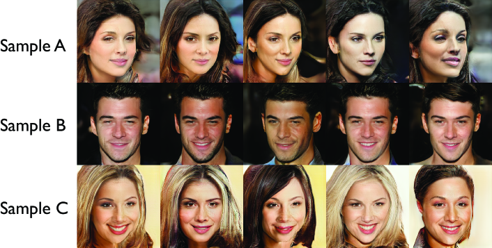
Figure 12. Example images generated from PGAN. Each row corresponding to a different hidden distribution.

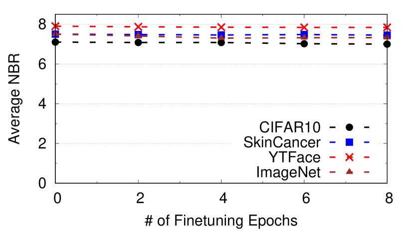
Figure 13. For adaptive attack that finetunes $F$ on benign data, average NBR of our system slightly decreases as the number of finetuning epochs increases.

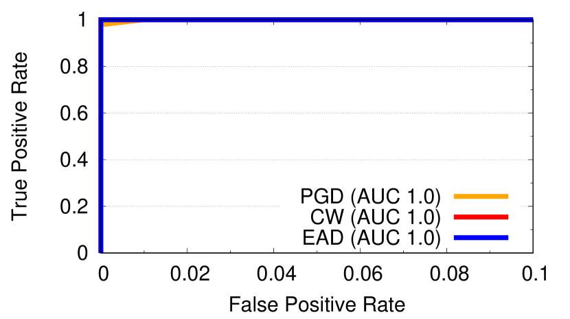
Figure 14. ROC curve of detecting adversarial examples generated using the $3$ adversarial attacks on CIFAR10. The x-axis is concatenated at 0.1 for brevity. (Single Leakage)

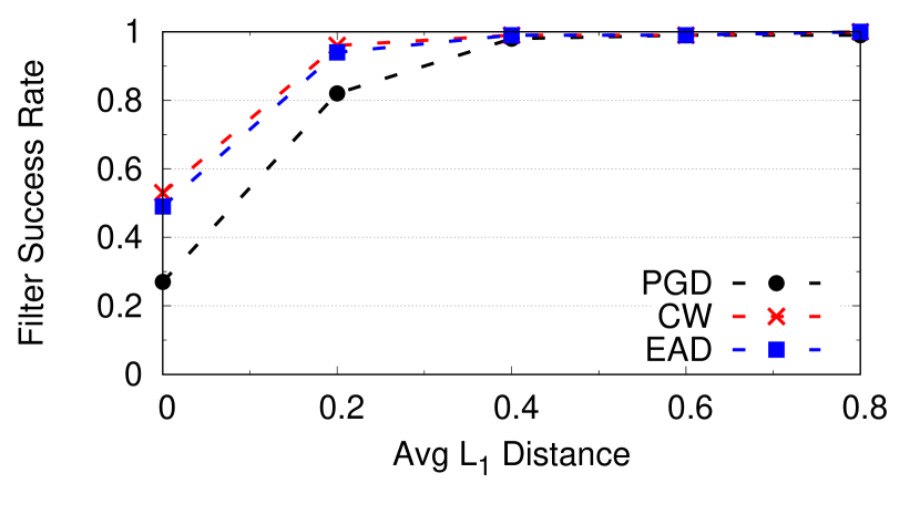
Figure 15. Analysis on the impact of selecting similar hidden distributions. The filter success rate increase rapidly as the $L_{1}$ distance between sampling Gaussian distributions increases.

A.1. Detailed Proof of Theorem 6.1

We now present the detailed proof of Theorem 6.1 described in §6. We start from presenting detailed definitions of attack optimization, transferability, and assumptions of $F$ and $G$, and then discuss how $G$ and its detector respond to an adversarial example computed from $F$.

Attack Optimization on $F$.    Let $x^{\prime}=x+\delta$ be an adversarial example optimized from model $F$ with target label $y_{t}$. We approximate $\ell_{2}$ loss around $x^{\prime}$ as loss of a linear classifier.

(7) $$\ell_{2}(F(x^{\prime}),y_{t})=(y_{t}-(a_{F}x^{\prime}+b_{F}))^{2}$$

We consider the perturbation $\delta$ to be optimized on $F$ for benign input $x$. Therefore, $\ell_{2}(F(x^{\prime}),y_{t})\leq\gamma$ for some small $\gamma>0$. This yields $\frac{y_{t}-b_{F}-\sqrt{\gamma}}{a_{F}}\leq x^{\prime}\leq\frac{y_{t}-b_{F}+\sqrt{\gamma}}{a_{F}}$.

Attack Transferability to $G$.    Let $G$ be a model being attacked by the adversarial example $(x^{\prime},y_{t})$. Similarly, the loss around $x^{\prime}$ on $G$ is approximated by

(8) $$\ell_{2}(G(x^{\prime}),y_{t})=(y_{t}-(a_{G}x^{\prime}+b_{G}))^{2}.$$

The adversarial example $x^{\prime}$ transfers to $G$ if its loss with respect to $y_{t}$ is bounded by some $\gamma^{\prime}$ such that $\ell_{2}(G(x^{\prime}),y_{t})\leq\gamma^{\prime}$. This yields $\frac{y_{t}-b_{G}-\sqrt{\gamma^{\prime}}}{a_{G}}\leq x^{\prime}\leq\frac{y_{t}-b_{G}+\sqrt{\gamma^{\prime}}}{a_{G}}$. Note that since $x^{\prime}$ is not optimized on $G$, naturally $\gamma^{\prime}>>\gamma$.

Assumptions on $F$ and $G$.    Since $F$ and $G$ are trained using the same benign training data, we assume $a_{F}=a_{G}=a$. On the other hand, $b_{F}\neq b_{G}$ due to the different hidden distributions. Without loss of generality, we assume $a>0$ and $b_{G}>b_{F}$. Our result remains the same when $b_{G}<b_{F}$.

How model $G$ and its attack detector respond to $x^{\prime}$.    There are two cases.

Case 1: If $b_{G}-b_{F}>\sqrt{\gamma^{\prime}}-\sqrt{\gamma}$, then $[\frac{y_{t}-b_{G}-\sqrt{\gamma^{\prime}}}{a_{G}},\frac{y_{t}-b_{G}+\sqrt{\gamma^{\prime}}}{a_{G}}]$ does not fully contain $[\frac{y_{t}-b_{F}-\sqrt{\gamma}}{a_{F}},\frac{y_{t}-b_{F}+\sqrt{\gamma}}{a_{F}}]$ and the adversarial example $x^{\prime}$ will not tranfer to $G$. In this case, $x^{\prime}$ can be easily identified since $F(x^{\prime})\neq G(x^{\prime})$.

Case 2: If $b_{G}-b_{F}\leq\sqrt{\gamma^{\prime}}-\sqrt{\gamma}$, then $[\frac{y_{t}-b_{F}-\sqrt{\gamma}}{a_{F}},\frac{y_{t}-b_{F}+\sqrt{\gamma}}{a_{F}}]$ is fully contained in $[\frac{y_{t}-b_{G}-\sqrt{\gamma^{\prime}}}{a_{G}},\frac{y_{t}-b_{G}+\sqrt{\gamma^{\prime}}}{a_{G}}]$. In this case, $x^{\prime}$ can cause $G(x^{\prime})=y_{t}$. This is when we use the filter defined by eq.(4) to compare the loss of $(x^{\prime},y_{t})$ between $F$ and $G$.

We now study $\ell_{2}(G(x^{\prime}),y_{t})-\ell_{2}(F(x^{\prime}),y_{t})$. Since $a_{F}=a_{G}=a$, we can expand the expression as:

$$\ell_{2}(G(x^{\prime}),y_{t})-\ell_{2}(F(x^{\prime}),y_{t})$$

$$= (y_{t}-(ax^{\prime}+b_{G}))^{2}-(y-(ax^{\prime}+b_{F}))^{2}$$

$$= 2y_{t}(ax^{\prime}+b_{F})-2y_{t}(ax^{\prime}+b_{G})+(ax^{\prime}+b_{G})^{2}-(ax^{\prime}+b_{F})^{2}$$

$$= 2y_{t}(b_{F}-b_{G})+2ax^{\prime}(b_{G}-b_{F})+b_{G}^{2}-b_{F}^{2}$$

Since $x^{\prime}$ lies in the interval of $[\frac{y_{t}-b_{F}-\sqrt{\gamma}}{a},\frac{y_{t}-b_{F}+\sqrt{\gamma}}{a}]$, we assume $x^{\prime}$ is uniformly distributed in this interval. Thus we have

$$\Pr(\ell_{2}(G(x^{\prime}),y_{t})-\ell_{2}(F(x^{\prime}),y_{t})>T)$$

$$= \Pr(2y_{t}(b_{F}-b_{G})+2ax^{\prime}(b_{G}-b_{F})+b_{G}^{2}-b_{F}^{2}>T)$$

$$= \Pr(x^{\prime}>\frac{T+b_{F}^{2}-b_{G}^{2}-2y_{t}(b_{F}-b_{G})}{2a(b_{G}-b_{F})})$$

$$= \frac{a}{2\sqrt{\gamma}}\left(\frac{y_{t}-b_{F}+\sqrt{\gamma}}{a}-\frac{T+b_{F}^{2}-b_{G}^{2}-2y_{t}(b_{F}-b_{G})}{2a(b_{G}-b_{F})}\right)$$

$$= \frac{a}{2\sqrt{\gamma}}\cdot\frac{(b_{G}-b_{F})(b_{G}-b_{F}+2\sqrt{\gamma})-T}{2a(b_{G}-b_{F})}$$

$$= \frac{(b_{G}-b_{F})(b_{G}-b_{F}+2\sqrt{\gamma})-T}{4\sqrt{\gamma}(b_{G}-b_{F})}$$

Let $\Pr(\ell_{2}(G(x^{\prime}),y_{t})-\ell_{2}(F(x^{\prime}),y_{t})>T)=p$, which yields $T=(b_{G}-b_{F})(b_{G}-b_{F}+2\sqrt{\gamma}-4\sqrt{\gamma}p)$. Now let $\mathcal{D}_{G,F}=b_{G}-b_{F}$, we have $T=\mathcal{D}_{G,F}\cdot(\mathcal{D}_{G,F}+2\sqrt{\gamma}-4\sqrt{\gamma}\cdot p)$.

This completes the proof of Theorem 6.1.

Discussion.    Note that Case 2 must meet the constraint of $b_{G}-b_{F}\leq\sqrt{\gamma^{\prime}}-\sqrt{\gamma}$. Thus if we train $F$ and $G$ to be “well-separated” when classifying non-benign inputs, we can set $b_{G}-b_{F}=\sqrt{\gamma^{\prime}}-\sqrt{\gamma}$. If $p=0.95$, $\frac{\gamma^{\prime}}{\gamma}=25$, then $T=8.8\gamma$.

Iterations	CIFAR10	SkinCancer	YTFace	ImageNet
1	7.3	—	—	7.7
10	6.9	7.2	7.7	7.4
50	7.1	7.5	7.8	7.5
100	7.1	7.5	7.9	7.5

Table 10. Average NBR of Neo against PGD attack first decrease and then increases slightly as the optimization iterations of PGD attack increases.

A.2. Implementation Details

Soft Nearest Neighbor Loss Term.    For each label in $L$, we calculate the SNNL loss term as the following:

(9) $$SNNL(X,Y)=-\frac{1}{N}\sum_{i\in 1..N}log\left(\frac{\sum\limits_{\begin{subarray}{c}j\in 1..N\\ j\neq i\\ y_{i}=y_{j}\end{subarray}}e^{-||x_{i}-x_{j}||^{2}}}{\sum\limits_{\begin{subarray}{c}k\in 1..N\\ k\neq i\end{subarray}}e^{-||x_{i}-x_{k}||^{2}}}\right)$$

$N$ is the total number of training data, $x_{i}$ is the i-th training data. The equation effectively minimize the distance of training data that are from the same dataset, while maxmizing distance of training data that are different classes.

Generating Hidden Distribution using GAN   . We use a GAN (Karras et al., 2017) trained on CelebA dataset (Liu et al., 2018). The GAN takes in an input vector of size $512$ and output a $224\times 224$ facial image. The GAN is trained with input vectors sampled from a Gaussian ball $\mathcal{N}(\mu=0,\,\sigma^{2}=1)$. For each hidden distribution, we sample from a smaller Gaussian ball within the original Gaussian ball that has a random mean vector (bounded between $-0.5$ and $0.5$) and a small standard deviation ($\sigma_{0}$). Then we query the GAN using noise vector sampled from the smaller Gaussian ball and take the generated images as the current hidden distribution. We empirically choose $\sigma_{0}=0.3$, which generates similar images but has enough variety as shown in Figure 12 in Appendix. In §7.2, we show that there exist a large number of hidden distributions in the GAN for our version generation purpose.

Next, we seek to estimate the total number of different hidden distributions exist in the GAN. To do so, we find the minimal separation that two versions needs to have in order to achieve high filter success rate. We train versions $F_{0}$ and $F_{1}$ using extremely similar hidden distributions (measured by the distance between the mean of Gaussian distributions used to sample the hidden distributions).

Figure 15 shows the filter success rate as the $L_{1}$ distance between the mean of the input Gaussian distributions (e.g., 512-long vectors) used to sample $F_{0}$ and $F_{1}$’s hidden distributions increases. We see that as long as $L_{1}$ distance between the sampling Gaussian distribution is above $0.4$, Neo can maintain $>98\%$ filter success rate. For reference, the maximum $L_{1}$ distance between the mean of two input Gaussian distribution is $512$. Note that even when $F_{0}$ and $F_{1}$ uses the exact same hidden distributions ($L_{1}=0$) the filter success rate is higher than zero. This is because the stochasticity of floating point GPU computation causes versions to be slightly different even the training data and parameter initialization is identical. Since our space of input Gaussian distribution is large ($512$ dimensions, each continuous from $-0.5$ to $0.5$), we have a large number of possible hidden distributions ($\geq 2^{512}$).

References

- (1)
- Abdelnabi and Fritz (2021) Sahar Abdelnabi and Mario Fritz. 2021. What’s in the box: Deflecting Adversarial Attacks by Randomly Deploying Adversarially-Disjoint Models. In Proc. of MTD. 3–12.
- Akhtar et al. (2021) Naveed Akhtar, Ajmal Mian, Navid Kardan, and Mubarak Shah. 2021. Advances in adversarial attacks and defenses in computer vision: A survey. IEEE Access 9 (2021), 155161–155196.
- Athalye et al. (2018) Anish Athalye, Nicholas Carlini, and David Wagner. 2018. Obfuscated gradients give a false sense of security: Circumventing defenses to adversarial examples. In Proc. of ICML. PMLR, 274–283.
- Bernard et al. (2017) Tara Bernard, Tiffany Hsu, Nicole Perlroth, and Ron Lieber. 2017. Equifax Says Cyberattack May Have Affected 143 Million in the U.S. https://www.nytimes.com/2017/09/07/business/equifaxcyberattack.html..
- Bourtoule et al. (2021) Lucas Bourtoule, Varun Chandrasekaran, Christopher A Choquette-Choo, Hengrui Jia, Adelin Travers, Baiwu Zhang, David Lie, and Nicolas Papernot. 2021. Machine unlearning. In Proc. of IEEE S&P. IEEE, 141–159.
- broadcom.com (2022) broadcom.com. 2022. Stop Threats in Their Tracks Wherever They Attack. https://www.broadcom.com/products/cyber-security/endpoint.
- Bryniarski et al. (2021) Oliver Bryniarski, Nabeel Hingun, Pedro Pachuca, Vincent Wang, and Nicholas Carlini. 2021. Evading adversarial example detection defenses with orthogonal projected gradient descent. arXiv preprint arXiv:2106.15023 (2021).
- Byun et al. (2022) Junyoung Byun, Seungju Cho, Myung-Joon Kwon, Hee-Seon Kim, and Changick Kim. 2022. Improving the Transferability of Targeted Adversarial Examples through Object-Based Diverse Input. arXiv preprint arXiv:2203.09123 (2022).
- Carlini (2020) Nicholas Carlini. 2020. A partial break of the honeypots defense to catch adversarial attacks. arXiv preprint arXiv:2009.10975 (2020).
- Carlini and Wagner (2016) Nicholas Carlini and David Wagner. 2016. Defensive distillation is not robust to adversarial examples. arXiv preprint arXiv:1607.04311 (2016).
- Carlini and Wagner (2017a) Nicholas Carlini and David Wagner. 2017a. Magnet and efficient defenses against adversarial attacks are not robust to adversarial examples. arXiv preprint arXiv:1711.08478 (2017).
- Carlini and Wagner (2017b) Nicholas Carlini and David Wagner. 2017b. Towards evaluating the robustness of neural networks. In Proc. of IEEE S&P.
- Chakraborty et al. (2018) Anirban Chakraborty, Manaar Alam, Vishal Dey, Anupam Chattopadhyay, and Debdeep Mukhopadhyay. 2018. Adversarial attacks and defences: A survey. arXiv preprint arXiv:1810.00069 (2018).
- Chen et al. (2020) Jianbo Chen, Michael I Jordan, and Martin J Wainwright. 2020. Hopskipjumpattack: A query-efficient decision-based attack. In Proc. of IEEE S&P. IEEE, 1277–1294.
- Chen et al. (2018) Pin-Yu Chen, Yash Sharma, Huan Zhang, Jinfeng Yi, and Cho-Jui Hsieh. 2018. EAD: elastic-net attacks to deep neural networks via adversarial examples. In Proc. of AAAI.
- Cohen et al. (2019) Jeremy Cohen, Elan Rosenfeld, and Zico Kolter. 2019. Certified Adversarial Robustness via Randomized Smoothing. In Proc. of ICML.
- Cone et al. (2007) Benjamin D Cone, Cynthia E Irvine, Michael F Thompson, and Thuy D Nguyen. 2007. A video game for cyber security training and awareness. computers & security 26, 1 (2007), 63–72.
- Demontis et al. (2019) Ambra Demontis, Marco Melis, Maura Pintor, Matthew Jagielski, Battista Biggio, Alina Oprea, Cristina Nita-Rotaru, and Fabio Roli. 2019. Why do adversarial attacks transfer? explaining transferability of evasion and poisoning attacks. In Proc. of USENIX Security. 321–338.
- Deng et al. (2009) Jia Deng, Wei Dong, Richard Socher, Li-Jia Li, Kai Li, and Li Fei-Fei. 2009. Imagenet: A large-scale hierarchical image database. In Proc. of CVPR. IEEE, 248–255.
- Duy et al. (2021) Kha Dinh Duy, Taehyun Noh, Siwon Huh, and Hojoon Lee. 2021. Confidential Machine Learning Computation in Untrusted Environments: A Systems Security Perspective. IEEE Access 9 (2021), 168656–168677.
- Frosst et al. (2019) Nicholas Frosst, Nicolas Papernot, and Geoffrey Hinton. 2019. Analyzing and improving representations with the soft nearest neighbor loss. In Proc. of ICML. PMLR, 2012–2020.
- Gao and Wu (2022) Chenxiang Gao and Wei Wu. 2022. Boosting the Transferability of Adversarial Examples with More Efficient Data Augmentation. In Journal of Physics, Vol. 2189. IOP Publishing, 012025.
- Goodfellow et al. (2014) Ian Goodfellow, Jean Pouget-Abadie, Mehdi Mirza, Bing Xu, David Warde-Farley, Sherjil Ozair, Aaron Courville, and Yoshua Bengio. 2014. Generative adversarial nets. Proc. of NeurIPS (2014).
- Gowal et al. (2020) Sven Gowal, Chongli Qin, Jonathan Uesato, Timothy Mann, and Pushmeet Kohli. 2020. Uncovering the limits of adversarial training against norm-bounded adversarial examples. arXiv preprint arXiv:2010.03593 (2020).
- Gowal et al. (2021) Sven Gowal, Sylvestre-Alvise Rebuffi, Olivia Wiles, Florian Stimberg, Dan Andrei Calian, and Timothy A Mann. 2021. Improving robustness using generated data.
- Guo et al. (2019) Chuan Guo, Tom Goldstein, Awni Hannun, and Laurens Van Der Maaten. 2019. Certified data removal from machine learning models. arXiv preprint arXiv:1911.03030 (2019).
- He et al. (2021) Chaoxiang He, Bin Benjamin Zhu, Xiaojing Ma, Hai Jin, and Shengshan Hu. 2021. Feature-Indistinguishable Attack to Circumvent Trapdoor-Enabled Defense. In Proc. of CCS. 3159–3176.
- He et al. (2016) Kaiming He, Xiangyu Zhang, Shaoqing Ren, and Jian Sun. 2016. Deep residual learning for image recognition. In Proc. of CVPR.
- Hoque et al. (2012) Mohammad Sazzadul Hoque, Md Mukit, Md Bikas, Abu Naser, et al. 2012. An implementation of intrusion detection system using genetic algorithm. arXiv preprint arXiv:1204.1336 (2012).
- Hu et al. (2021) Xing Hu, Ling Liang, Lei Deng, Yu Ji, Yufei Ding, Zidong Du, Qi Guo, Timothy Sherwood, Yuan Xie, et al. 2021. A systematic view of leakage risks in deep neural network systems. (2021).
- Hua et al. (2018) Weizhe Hua, Zhiru Zhang, and G Edward Suh. 2018. Reverse engineering convolutional neural networks through side-channel information leaks. In Proc. of DAC. IEEE, 1–6.
- Huang et al. (2017) Gao Huang, Zhuang Liu, Laurens Van Der Maaten, and Kilian Q Weinberger. 2017. Densely connected convolutional networks. In Proc. of CVPR. 4700–4708.
- Jakobsson (2005) Markus Jakobsson. 2005. Modeling and preventing phishing attacks. In Financial Cryptography, Vol. 5. Citeseer.
- Jibilian and Canales (2021) I Jibilian and K Canales. 2021. The US is readying sanctions against Russia over the solarwinds cyber attack. Here’s a simple explanation of how the massive hack happened and why it’s such a big deal.
- Kariyappa and Qureshi (2019) Sanjay Kariyappa and Moinuddin K Qureshi. 2019. Improving adversarial robustness of ensembles with diversity training. arXiv preprint arXiv:1901.09981 (2019).
- Karras et al. (2017) Tero Karras, Timo Aila, Samuli Laine, and Jaakko Lehtinen. 2017. Progressive growing of gans for improved quality, stability, and variation. Proc. of ICLR (2017).
- King (2020) Jeff King. 2020. How We Review Content.
- Kingma and Ba (2014) Diederik P Kingma and Jimmy Ba. 2014. Adam: A method for stochastic optimization. arXiv preprint arXiv:1412.6980 (2014).
- Kolter and Wong (2017) J. Zico Kolter and Eric Wong. 2017. Provable defenses against adversarial examples via the convex outer adversarial polytope. In Proc. of NeurIPS.
- Krizhevsky and Hinton (2009) Alex Krizhevsky and Geoffrey Hinton. 2009. Learning multiple layers of features from tiny images. Technical Report.
- Kurakin et al. (2016) Alexey Kurakin, Ian Goodfellow, and Samy Bengio. 2016. Adversarial examples in the physical world. arXiv preprint arXiv:1607.02533 (2016).
- Li et al. (2022) Huiying Li, Shawn Shan, Emily Wenger, Jiayun Zhang, Haitao Zheng, and Ben Y Zhao. 2022. Blacklight: Scalable Defense for Neural Networks against Query-Based Black-Box Attacks. In Proc. of USENIX Security. Boston, MA.
- Liao et al. (2013) Hung-Jen Liao, Chun-Hung Richard Lin, Ying-Chih Lin, and Kuang-Yuan Tung. 2013. Intrusion detection system: A comprehensive review. Journal of Network and Computer Applications 36, 1 (2013), 16–24.
- Liu et al. (2016) Yanpei Liu, Xinyun Chen, Chang Liu, and Dawn Song. 2016. Delving into transferable adversarial examples and black-box attacks. arXiv preprint arXiv:1611.02770 (2016).
- Liu et al. (2018) Ziwei Liu, Ping Luo, Xiaogang Wang, and Xiaoou Tang. 2018. Large-scale celebfaces attributes (celeba) dataset. Retrieved August 15, 2018 (2018), 11.
- Madry et al. (2018) Aleksander Madry, Aleksandar Makelov, Ludwig Schmidt, Dimitris Tsipras, and Adrian Vladu. 2018. Towards deep learning models resistant to adversarial attacks. In Proc. of ICLR.
- Meng and Chen (2017) Dongyu Meng and Hao Chen. 2017. Magnet: a two-pronged defense against adversarial examples. In Proc. of CCS.
- Mink et al. (2022) Jaron Mink, Licheng Luo, Natã M Barbosa, Olivia Figueira, Yang Wang, and Gang Wang. 2022. DeepPhish: Understanding User Trust Towards Artificially Generated Profiles in Online Social Networks. In Proc. of USENIX Security.
- mitre.org (2022) mitre.org. 2022. MITRE Matrix. https://attack.mitre.org/matrices/enterprise/..
- Moon et al. (2019) Seungyong Moon, Gaon An, and Hyun Oh Song. 2019. Parsimonious black-box adversarial attacks via efficient combinatorial optimization. In Proc. of ICML. PMLR, 4636–4645.
- Moosavi-Dezfooli et al. (2016) Seyed-Mohsen Moosavi-Dezfooli, Alhussein Fawzi, and Pascal Frossard. 2016. Deepfool: a simple and accurate method to fool deep neural networks. In Proc. of CVPR. 2574–2582.
- Papernot et al. (2017) Nicolas Papernot, Patrick McDaniel, Ian Goodfellow, Somesh Jha, Z. Berkay Celik, and Ananthram Swami. 2017. Practical black-box attacks against machine learning. In Proc. of AsiaCCS.
- Papernot et al. (2016) N. Papernot, P. McDaniel, X. Wu, S. Jha, and A. Swami. 2016. Distillation as a defense to adversarial perturbations against deep neural networks. In Proc. of IEEE S&P.
- Qin et al. (2021) Yunxiao Qin, Yuanhao Xiong, Jinfeng Yi, and Cho-Jui Hsieh. 2021. Adversarial Attack across Datasets. arXiv preprint arXiv:2110.07718 (2021).
- Rakin et al. (2021) Adnan Siraj Rakin, Md Hafizul Islam Chowdhuryy, Fan Yao, and Deliang Fan. 2021. Deepsteal: Advanced model extractions leveraging efficient weight stealing in memories. arXiv preprint arXiv:2111.04625 (2021).
- Rebuffi et al. (2021) Sylvestre-Alvise Rebuffi, Sven Gowal, Dan A Calian, Florian Stimberg, Olivia Wiles, and Timothy Mann. 2021. Fixing data augmentation to improve adversarial robustness. arXiv preprint arXiv:2103.01946 (2021).
- Ribeiro et al. (2015) Mauro Ribeiro, Katarina Grolinger, and Miriam AM Capretz. 2015. Mlaas: Machine learning as a service. In Proc. of ICMLA. IEEE, 896–902.
- Riley et al. (2014) Michael Riley, Ben Elgin, Dune Lawrence, and Carol Matlack. 2014. Missed alarms and 40 million stolen credit card numbers: How target blew it. Bloomberg Businessweek 13 (2014).
- Sabour et al. (2015) Sara Sabour, Yanshuai Cao, Fartash Faghri, and David J Fleet. 2015. Adversarial manipulation of deep representations. arXiv preprint arXiv:1511.05122 (2015).
- Sandler et al. (2018) Mark Sandler, Andrew Howard, Menglong Zhu, Andrey Zhmoginov, and Liang-Chieh Chen. 2018. Mobilenetv2: Inverted residuals and linear bottlenecks. In Proc. of CVPR. 4510–4520.
- Shafahi et al. (2019) Ali Shafahi, Mahyar Najibi, Mohammad Amin Ghiasi, Zheng Xu, John Dickerson, Christoph Studer, Larry S Davis, Gavin Taylor, and Tom Goldstein. 2019. Adversarial training for free!
- Shan et al. (2021) Shawn Shan, Arjun Nitin Bhagoji, Haitao Zheng, and Ben Y Zhao. 2021. Patch-based defenses against web fingerprinting attacks. In Proc. of AISec. 97–109.
- Shan et al. (2022) Shawn Shan, Arjun Nitin Bhagoji, Haitao Zheng, and Ben Y Zhao. 2022. Poison Forensics: Traceback of Data Poisoning Attacks in Neural Networks. Proc. of USENIX Security.
- Shan et al. (2020a) Shawn Shan, Emily Wenger, Bolun Wang, Bo Li, Haitao Zheng, and Ben Y Zhao. 2020a. Gotta Catch’Em All: Using Honeypots to Catch Adversarial Attacks on Neural Networks. In Proc. of CCS. 67–83.
- Shan et al. (2020b) Shawn Shan, Emily Wenger, Jiayun Zhang, Huiying Li, Haitao Zheng, and Ben Y Zhao. 2020b. Fawkes: Protecting privacy against unauthorized deep learning models. In Proc. of USENIX Security. 1589–1604.
- Srivastava et al. (2014) Nitish Srivastava, Geoffrey Hinton, Alex Krizhevsky, Ilya Sutskever, and Ruslan Salakhutdinov. 2014. Dropout: a simple way to prevent neural networks from overfitting. The journal of machine learning research 15, 1 (2014), 1929–1958.
- Sun et al. (2020) Zhichuang Sun, Ruimin Sun, Changming Liu, Amrita Roy Chowdhury, Somesh Jha, and Long Lu. 2020. ShadowNet: A secure and efficient system for on-device model inference. arXiv preprint arXiv:2011.05905 (2020).
- Szegedy et al. (2017) Christian Szegedy, Sergey Ioffe, Vincent Vanhoucke, and Alexander A Alemi. 2017. Inception-v4, inception-resnet and the impact of residual connections on learning. In Proc. of AAAI.
- Tan and Le (2019) Mingxing Tan and Quoc Le. 2019. Efficientnet: Rethinking model scaling for convolutional neural networks. In Proc. of ICML. PMLR, 6105–6114.
- Tramer et al. (2020) Florian Tramer, Nicholas Carlini, Wieland Brendel, and Aleksander Madry. 2020. On adaptive attacks to adversarial example defenses. Proc. of NeurIPS 33 (2020), 1633–1645.
- Tramèr et al. (2017) Florian Tramèr, Alexey Kurakin, Nicolas Papernot, Ian Goodfellow, Dan Boneh, and Patrick McDaniel. 2017. Ensemble adversarial training: Attacks and defenses. arXiv preprint arXiv:1705.07204 (2017).
- trustwave.com (2020) trustwave.com. 2020. Trustwave Global Security Report. https://www.trustwave.com/en-us/resources/library/documents/2020-trustwave-global-security-report/..
- Tschandl et al. (2018) Philipp Tschandl, Cliff Rosendahl, and Harald Kittler. 2018. The HAM10000 dataset, a large collection of multi-source dermatoscopic images of common pigmented skin lesions. Scientific data 5, 1 (2018), 1–9.
- Uesato et al. (2018) Jonathan Uesato, Brendan O’Donoghue, Aaron van den Oord, and Pushmeet Kohli. 2018. Adversarial risk and the dangers of evaluating against weak attacks. arXiv preprint arXiv:1802.05666 (2018).
- Vyas et al. (2018) Apoorv Vyas, Nataraj Jammalamadaka, Xia Zhu, Dipankar Das, Bharat Kaul, and Theodore L Willke. 2018. Out-of-distribution detection using an ensemble of self supervised leave-out classifiers. In Proc. of ECCV. 550–564.
- Wang and He (2021) Xiaosen Wang and Kun He. 2021. Enhancing the transferability of adversarial attacks through variance tuning. In Proc. of CVPR. 1924–1933.
- Wong et al. (2020) Eric Wong, Leslie Rice, and J Zico Kolter. 2020. Fast is better than free: Revisiting adversarial training. arXiv preprint arXiv:2001.03994 (2020).
- Wu et al. (2018) Lei Wu, Zhanxing Zhu, Cheng Tai, and Weinan E. 2018. Understanding and enhancing the transferability of adversarial examples. arXiv preprint arXiv:1802.09707 (2018).
- Xie et al. (2019) Cihang Xie, Zhishuai Zhang, Yuyin Zhou, Song Bai, Jianyu Wang, Zhou Ren, and Alan L Yuille. 2019. Improving transferability of adversarial examples with input diversity. In Proc. of CVPR. 2730–2739.
- Xu et al. (2021) Teng Xu, Gerard Goossen, Huseyin Kerem Cevahir, Sara Khodeir, Yingyezhe Jin, Frank Li, Shawn Shan, Sagar Patel, David Freeman, and Paul Pearce. 2021. Deep entity classification: Abusive account detection for online social networks. In Proc. of USENIX Security.
- Yang et al. (2020) Huanrui Yang, Jingyang Zhang, Hongliang Dong, Nathan Inkawhich, Andrew Gardner, Andrew Touchet, Wesley Wilkes, Heath Berry, and Hai Li. 2020. DVERGE: diversifying vulnerabilities for enhanced robust generation of ensembles. Proc. of NeurIPS 33 (2020), 5505–5515.
- Yang et al. (2021) Zhuolin Yang, Linyi Li, Xiaojun Xu, Shiliang Zuo, Qian Chen, Pan Zhou, Benjamin Rubinstein, Ce Zhang, and Bo Li. 2021. TRS: Transferability Reduced Ensemble via Promoting Gradient Diversity and Model Smoothness. Proc. of NeurIPS (2021).
- Yao et al. (2017) Yuanshun Yao, Zhujun Xiao, Bolun Wang, Bimal Viswanath, Haitao Zheng, and Ben Y. Zhao. 2017. Complexity vs. Performance: Empirical Analysis of Machine Learning as a Service. In Proc. of IMC. London, UK.
- YouTube (2011) YouTube 2011. https://www.cs.tau.ac.il/~wolf/ytfaces/. YouTube Faces DB.
- Yu et al. (2020) Honggang Yu, Kaichen Yang, Teng Zhang, Yun-Yun Tsai, Tsung-Yi Ho, and Yier Jin. 2020. CloudLeak: Large-Scale Deep Learning Models Stealing Through Adversarial Examples. In Proc. of NDSS.
- Yuan et al. (2022) Xiaoyong Yuan, Leah Ding, Lan Zhang, Xiaolin Li, and Dapeng Oliver Wu. 2022. ES attack: Model stealing against deep neural networks without data hurdles. IEEE Trans. on ETCI (2022).
- Zantedeschi et al. (2017) Valentina Zantedeschi, Maria-Irina Nicolae, and Ambrish Rawat. 2017. Efficient defenses against adversarial attacks. In Proc. of AISec.
- Zeiler (2012) Matthew D Zeiler. 2012. Adadelta: an adaptive learning rate method. arXiv preprint arXiv:1212.5701 (2012).
- Zhang et al. (2019) Hongyang Zhang, Yaodong Yu, Jiantao Jiao, Eric Xing, Laurent El Ghaoui, and Michael Jordan. 2019. Theoretically principled trade-off between robustness and accuracy. In Proc. of ICML. PMLR, 7472–7482.
- Zheng et al. (2016) Stephan Zheng, Yang Song, Thomas Leung, and Ian Goodfellow. 2016. Improving the robustness of deep neural networks via stability training. In Proc. of CVPR.
- Zhou et al. (2021) Yan Zhou, Murat Kantarcioglu, and Bowei Xi. 2021. Exploring the Effect of Randomness on Transferability of Adversarial Samples against Deep Neural Networks. IEEE Transactions on Dependable and Secure Computing (2021).