Are Message Passing Neural Networks Really Helpful for Knowledge Graph Completion?

Abstract

Knowledge graphs (KGs) facilitate a wide variety of applications. Despite great efforts in creation and maintenance, even the largest KGs are far from complete. Hence, KG completion (KGC) has become one of the most crucial tasks for KG research. Recently, considerable literature in this space has centered around the use of Message Passing (Graph) Neural Networks (MPNNs), to learn powerful embeddings. The success of these methods is naturally attributed to the use of MPNNs over simpler multi-layer perceptron (MLP) models, given their additional message passing (MP) component. In this work, we find that surprisingly, simple MLP models are able to achieve comparable performance to MPNNs, suggesting that MP may not be as crucial as previously believed. With further exploration, we show careful scoring function and loss function design has a much stronger influence on KGC model performance. This suggests a conflation of scoring function design, loss function design, and MP in prior work, with promising insights regarding the scalability of state-of-the-art KGC methods today, as well as careful attention to more suitable MP designs for KGC tasks tomorrow. Our codes are publicly available at: https://github.com/Juanhui28/Are_MPNNs_helpful.

1 Introduction

Knowledge graphs (KGs) (Bollacker et al., 2008; Carlson et al., 2010) are a type of knowledge base, which store multi-relational factual knowledge in the form of triplets. Each triplet specifies the relation between a head and a tail entity. KGs conveniently capture rich structured knowledge about many types of entities (e.g. objects, events, concepts) and thus facilitate numerous applications such as information retrieval (Xiong et al., 2017a), recommender systems (Wang et al., 2019), and question answering (West et al., 2014). To this end, the adopted KGs are expected to be as comprehensive as possible to provide all kinds of required knowledge. However, existing large-scale KGs are known to be far from complete with large portions of triplets missing (Bollacker et al., 2008; Carlson et al., 2010). Imputing these missing triplets is of great importance. Furthermore, new knowledge (triplets) is constantly emerging even between existing entities, which also calls for dedicated efforts to predict these new triplets (García-Durán et al., 2018; Jin et al., 2019). Therefore, knowledge graph completion (KGC) is a problem of paramount importance (Lin et al., 2015; Yu et al., 2021). A crucial step towards better KGC performance is to learn low-dimensional continuous embeddings for both entities and relations (Bordes et al., 2013).

Recently, due to the intrinsic graph-structure of KGs, Graph Neural Networks (GNNs) have been adopted to learning more powerful embeddings for their entities and relations, and thus facilitate the KGC. There are mainly two types of GNN-based KGC methods: Message Passing Neural Networks (MPNNs) (Schlichtkrull et al., 2018; Vashishth et al., 2020) and path-based methods (Zhu et al., 2021; Zhang and Yao, 2022; Zhu et al., 2022). In this work, we focus on MPNN-based models, which update node features through a message passing (MP) process over the graph where each node collects and transforms features from its neighbors. When adopting MPNNs for KGs, dedicated efforts are often devoted to developing more sophisticated MP processes that are customized for better capturing multi-relational information (Vashishth et al., 2020; Schlichtkrull et al., 2018; Ye et al., 2019). The improvement brought by MPNN-based models is thus naturally attributed to these enhanced MP processes. Therefore, current research on developing better MPNNs for KGs is still largely focused on advancing MP processes.

Present Work. In this work, we find that, surprisingly, the MP in the MPNN-based models is not the most critical reason for reported performance improvements for KGC. Specifically, we replaced MP in several state-of-the-art KGC-focused MPNN models such as RGCN (Schlichtkrull et al., 2018), CompGCN (Vashishth et al., 2020) and KBGAT (Nathani et al., 2019) with simple Multiple Layer Perceptrons (MLPs) and achieved comparable performance to their corresponding MPNN-based models, across a variety of datasets and implementations. We carefully scrutinized these MPNN-based models and discovered they also differ from each other in other key components such as scoring functions and loss functions. To better study how these components contribute to the model, we conducted comprehensive experiments to demonstrate the effectiveness of each component. Our results indicate that the scoring and loss functions have stronger influence while MP makes almost no contributions. Based on our findings, we develop ensemble models built upon MLPs, which are able to achieve better performance than MPNN-based models; these implications are powerful in practice, given scalability advantages of MLPs over MPNNs (Zhang et al., 2022a).

2 Preliminaries

Before moving to main content, we first introduce KGC-related preliminaries, five datasets and three MPNN-based models we adopt for investigations.

2.1 Knowledge graph completion (KGC)

The task of KGC is to infer missing triplets based on known facts in the KG. In KGC, we aim to predict a missing head or tail entity given a triplet. Specifically, we denote the triplets with missing head (tail) entity as $(h,r,?)$ ($(?,r,t)$), where the question mark indicates the entity we aim to predict. Since the head entity prediction and tail entity prediction tasks are symmetric, in the following, we only use the tail entity prediction task for illustration. When conducting the KGC task for a triplet $(h,r,?)$, we use all entities in KG as candidates and try to select the best one as the tail entity. Typically, for each candidate entity $t^{\prime}$, we evaluate its score for the triplet $(h,r,t^{\prime})$ with the function $s_{h,r}(t^{\prime})=f(h,r,t^{\prime})$, where $s_{h,r}(t^{\prime})$ is the score of $t^{\prime}$ given the head entity $h$ and the relation $r$, and $f$ is a scoring function. We choose the entity $t^{\prime}$ with the largest score as the predicted tail entity. $f(\cdot)$ can be modeled in various ways as discussed later.

Datasets. We use five well-known KG datasets, i.e., FB15k Bordes et al. (2013), FB15k-237 Toutanova et al. (2015); Toutanova and Chen (2015), WN18 Schlichtkrull et al. (2018), WN18RR Dettmers et al. (2018) and NELL-995 (Xiong et al., 2017b) for this study. The detailed descriptions and data statistics can be found in Appendix A. Following the settings in previous works (Vashishth et al., 2020; Schlichtkrull et al., 2018), triplets in these datasets are randomly split into training, validation, and test sets, denoted $\mathcal{D}_{train},\mathcal{D}_{val},\mathcal{D}_{test}$, respectively. The triplets in the training set are regarded as the known facts. We manually remove the head/tail entity of the triplets in the validation and test sets for model selection and evaluation. Specifically, for the tail entity prediction task, given a triplet $(h,r,t^{*})$, we remove $t^{*}$ and construct a test sample $(h,r,?)$. The tail entity $t^{*}$ is regarded as the ground-truth for this sample.

Evaluation Metrics. When evaluating the performance, we focus on the predicted scores for the ground-truth entity of the triplets in the test set $\mathcal{D}_{test}$. For each triplet $(h,r,?)$ in the test set, we sort all candidate entities $t$ in a non-increasing order according to $s_{h,r}(t)$. Then, we use the rank-based measures to evaluate the prediction quality, including Mean Reciprocal Rank (MRR) and Hits@N. In this work, we choose $N\in\{1,3,10\}$. See Appendix B for their definitions.

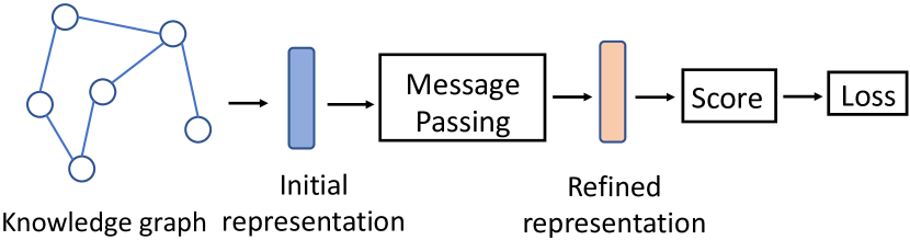
Figure 1: A general MPNN framework for KGC.

2.2 MPNN-based KGC

Various MPNN-based models have been utilized for KGC by learning representations for the entities and relations of KGs. The learnt representations are then used as input to a scoring function $f(\cdot)$. Next, we first introduce MPNN models specifically designed for KG. Then, we introduce scoring functions. Finally, we describe the training process, including loss functions.

2.2.1 MPNNs for learning KG representations

KGs can be naturally treated as graphs with triplets being the relational edges. When MPNN models are adapted to learn representations for KGs, the MP process in the MPNN layers is tailored for handling such relational data (triplets). In this paper, we investigate three representative MPNN-based models for KGC, i.e., CompGCN Vashishth et al. (2020), RGCN Schlichtkrull et al. (2018) and KBGAT (Nathani et al., 2019), which are most widely adopted. As in standard MPNN models, these models stack multiple layers to iteratively aggregate information throughout the KG. Each intermediate layer takes the output from the previous layer as the input, and the final output from the last layer serves as the learned embeddings. In addition to entity embeddings, some MPNN-based models also learn relation embeddings. For a triplet $(h,r,t)$, we use ${\bf x}^{(k)}_{h}$, ${\bf x}^{(k)}_{r}$, and ${\bf x}^{(k)}_{t}$ to denote the head, relation, and tail embeddings obtained after the $k$-th layer. Specifically, the input embeddings of the first layer ${\bf x}^{(0)}_{h}$ , ${\bf x}^{(0)}_{r}$ and ${\bf x}^{(0)}_{t}$ are randomly initialized. RGCN aggregates neighborhood information with the relation-specific transformation matrices. CompGCN defines direction-based transformation matrices and introduces relation embeddings to aggregate the neighborhood information. It introduces the composition operator to combine the embeddings to leverage the entity-relation information. KBGAT proposes attention-based aggregation process by considering both the entity embedding and relation embedding. More details about the MP process for CompGCN, RGCN and KBGAT can be found in Appendix C. For MPNN-based models with $K$ layers, we use ${\bf x}^{(K)}_{h}$, ${\bf x}^{(K)}_{r}$, and ${\bf x}^{(K)}_{t}$ as the final output embeddings and denote them as ${\bf x}_{h}$ , ${\bf x}_{r}$, and ${\bf x}_{t}$ for the simplicity of notations. Note that RGCN does not involve relation embedding ${\bf x}_{r}$ in the MP process, which will be randomly initialized if required by the scoring function.

2.2.2 Scoring functions

After obtaining the final embeddings from the MP layers, they are utilized as input to the scoring function $f$. Various scoring functions can be adopted. Two widely used scoring functions are DistMult (Yang et al., 2015) and ConvE (Dettmers et al., 2018). More specifically, RGCN adopts DistMult. In CompGCN, both scoring functions are investigated and ConvE is shown to be more suitable in most cases. Hence, in this paper, we use ConvE as the default scoring function for CompGCN. See Appendix D for more scoring function details.

2.2.3 Training MPNN-based models for KGC

To train the MPNN model, the KGC task is often regarded as a binary classification task to differentiate the true triplets from the randomly generated “fake” triplets. During training, all triplets in $\mathcal{D}_{train}$ and the corresponding inverse triplets $\mathcal{D}^{\prime}_{train}=\{(t,r_{in},h)|(h,r,t)\in\mathcal{D}_{train}\}$ are treated as positive samples, where $r_{in}$ is the inverse relation of $r$. The final positive sample set can be denoted as $\mathcal{D}^{*}_{train}=\mathcal{D}_{train}\bigcup\mathcal{D}^{\prime}_{train}$. Negative samples are generated by corrupting the triplets in $\mathcal{D}^{*}_{train}$. Specifically, for a triplet $(e_{1},rel,e_{2})\in\mathcal{D}^{*}_{train}$, we corrupt it by replacing its tail entities with other entities in the KG. More formally, the set of negative samples corresponding to the triplet $(e_{1},rel,e_{2})$ is denoted as: $\mathcal{C}_{(e_{1},rel,e_{2})}=\{(e_{1},rel,e_{2}^{\prime})|e_{2}^{\prime}\in\mathcal{V},e_{2}^{\prime}\neq e_{2}\}$ where $\mathcal{V}$ is the set of entities in KG. CompGCN uses $\mathcal{C}_{(e_{1},rel,e_{2})}$ as the negative samples. However, not all negative samples are utilized for training the RGCN model. Instead, for each positive sample triplet in $\mathcal{D}^{*}_{train}$, they adopt negative sampling to select $10$ such samples from $\mathcal{C}_{(e_{1},rel,e_{2})}$, and use only these for training. Also, for RGCN, any relation ${r}$ and its inverse relation $r_{in}$ share the same diagonal matrix for DistMult in Eq. (5) in Appendix D. Both CompGCN and RGCN adopt the Binary Cross-Entropy (BCE) loss. More details are given in Appendix E.

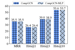
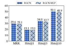
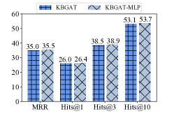
Figure 2: KGC results (%) of CompGCN/CompGCN-MLP, RGCN/RGCN-MLP, and KBGAT/KBGAT-MLP on FB15K-237. The MLP counterparts achieve compare performance as the corresponding MPNN models.

2.2.4 Major differences between MPNNs

We demonstrate an overview of MPNN-based model frameworks for the KGC task in Figure 1. Specifically, the framework consists of several key components including the MP (introduced in Section 2.2.1), the scoring function (2.2.2), and the loss function ( 2.2.3). Training can typically be conducted end-to-end. Both RGCN and CompGCN follow this framework with various designs in each component. We provide a more detailed comparison about them later in this section. However, KBGAT adopts a two-stage training process, which separates the training of the MP process (representation learning) and the scoring function. KBGAT achieves strong performance as reported in the original paper Nathani et al. (2019), which was later attributed to a test leakage issue Sun et al. (2020). After addressing this test leakage issue, we found that fitting KBGAT into the general framework described in Figure 1 leads to much higher performance than training it with the two-stage process (around $10\%$ improvement on FB15K-237). Hence, in this paper, we conduct analyses for KBGAT by fitting its MP process (described in Appendix C) into the framework described in Figure 1.

We summarize the major differences between RGCN, CompGCN, and KBGAT across three major components: (1) Message Passing. Their MP processes are different as described in Section 2.2.1 and detailed in Appendix C. (2) Scoring Function. They adopt different scoring functions. RGCN adopts the DistMult scoring function while CompGCN achieves best performance with ConvE. Thus, in this paper, we use ConvE as its default scoring function. For KBGAT, we adopt ConvE as its default scoring function. (3) Loss Function. As described in Section 2.2.3, CompGCN utilizes all entities in the KG as negative samples for training, while RGCN adopts a negative sampling strategy. For KBGAT, we also utilize all entities to construct negative samples, similar to CompGCN.

3 What Matters for MPNN-based KGC?

Recent efforts in adapting MPNN models for KG mostly focus on designing more sophisticated MP components to better handle multi-relational edges. These recently proposed MPNN-based methods have reported strong performance on the KGC task. Meanwhile, RGCN, CompGCN and KBGAT achieve different performance. Their strong performance compared to traditional embedding based models and their performance difference are widely attributed to the MP components Schlichtkrull et al. (2018); Vashishth et al. (2020); Nathani et al. (2019). However, as summarized in Section 2.2.4, they differ from each other in several ways besides MP; little attention has been paid to understand how each component affects these models. Thus, what truly matters for MPNN-based KGC performance is still unclear. To answer this question, we design careful experiments to ablate the choices of these components in RGCN, CompGCN and KBGAT to understand their roles, across multiple datasets. All reported results are mean and standard deviation over three seeds. Since MP is often regarded as the major contributor, we first investigate: is MP really helpful? Subsequently, we study the impact of the scoring function and the loss function.

Table 1: KGC results (%) with various scoring functions. Models behave differently with different scoring functions.

FB15K-237 WN18RR NELL-995 MRR Hits@1 Hits@3 Hits@10 MRR Hits@1 Hits@3 Hits@10 MRR Hits@1 Hits@3 Hits@10 CompGCN DistMult 33.7$\pm$ 0.1 24.7$\pm$0.1 36.9$\pm$0.2 51.5$\pm$0.2 42.9$\pm$0.1 39.0$\pm$0.1 43.9$\pm$0.1 51.7$\pm$0.3 32.3$\pm$0.5 24.3$\pm$0.6 36.1$\pm$0.4 47.4$\pm$0.2 ConvE 35.5$\pm$0.1 26.4$\pm$0.1 39.0$\pm$0.2 53.6$\pm$0.3 47.2$\pm$0.2 43.7$\pm$0.3 48.5$\pm$0.3 54.0$\pm$0.0 38.1$\pm$0.4 30.4$\pm$ 0.5 42.2$\pm$0.3 52.9$\pm$ 0.1 RGCN DistMult 29.6$\pm$0.3 19.1$\pm$0.5 34.0$\pm$ 0.2 50.1$\pm$0.2 43.0$\pm$0.2 38.6$\pm$0.3 45.0$\pm$0.1 50.8$\pm$0.3 27.8$\pm$0.2 19.9$\pm$0.2 31.4$\pm$0.0 43.0$\pm$0.3 ConvE 29.6$\pm$0.4 20.3$\pm$ 0.4 32.7$\pm$0.5 47.9$\pm$0.6 28.9$\pm$ 0.7 17.4$\pm$ 0.8 36.9$\pm$0.5 48.8$\pm$0.5 31.7$\pm$0.2 23.3$\pm$0.2 35.3$\pm$0.3 48.5$\pm$ 0.2 KBGAT DistMult 33.4$\pm$0.1 24.5$\pm$0.1 36.6$\pm$0.1 51.3$\pm$0.5 42.1$\pm$0.4 38.7$\pm$0.4 43.1$\pm$ 0.6 49.6$\pm$0.6 33.0$\pm$0.2 25.5$\pm$ 0.1 36.8$\pm$ 0.5 47.3$\pm$0.5 ConvE 35.0$\pm$0.3 26.0$\pm$0.3 38.5$\pm$ 0.3 53.1$\pm$ 0.3 46.4$\pm$0.2 42.6$\pm$0.2 47.9$\pm$0.3 53.9$\pm$0.2 37.4$\pm$0.6 29.7$\pm$0.7 41.4$\pm$ 0.8 52.0$\pm$0.4

Table 2: KGC results (%) with various loss functions. The loss function significantly impacts model performance.

FB15K-237 WN18RR NELL-995 MRR Hits@1 Hits@3 Hits@10 MRR Hits@1 Hits@3 Hits@10 MRR Hits@1 Hits@3 Hits@10 CompGCN with 31.5$\pm$0.1 22.2$\pm$0.1 34.8$\pm$0.2 49.6$\pm$0.2 32.9$\pm$ 0.9 24.4$\pm$ 1.5 39.0$\pm$0.5 46.7$\pm$0.4 32.0$\pm$0.2 23.8$\pm$0.2 35.7$\pm$0.1 48.1$\pm$0.2 w/o 35.5$\pm$0.1 26.4$\pm$0.1 39.0$\pm$0.2 53.6$\pm$0.3 47.2$\pm$0.2 43.7$\pm$0.3 48.5$\pm$0.3 54.0$\pm$0.0 38.1$\pm$0.4 30.4$\pm$ 0.5 42.2$\pm$0.3 52.9$\pm$ 0.1 RGCN with 29.6$\pm$0.3 19.1$\pm$0.5 34.0$\pm$0.2 50.1$\pm$0.2 43.0$\pm$0.2 38.6$\pm$0.3 45.0$\pm$0.1 50.8$\pm$0.3 27.8$\pm$0.2 19.9$\pm$0.2 31.4$\pm$0.0 43.0$\pm$0.3 w/o 33.4 $\pm$ 0.1 24.3$\pm$ 0.1 36.7$\pm$0.1 51.4$\pm$ 0.2 44.5$\pm$ 0.1 40.9$\pm$0.1 45.5$\pm$ 0.1 51.8$\pm$ 0.2 34.6$\pm$ 0.6 27.0$\pm$ 0.6 38.3$\pm$ 0.6 49.4$\pm$ 0.6 KBGAT with 30.1$\pm$ 0.3 21.0$\pm$ 0.3 33.2$\pm$ 0.4 48.1$\pm$ 0.3 30.1$\pm$ 0.2 18.6 $\pm$0.3 37.8$\pm$0.3 49.8$\pm$0.2 32.6 $\pm$ 0.3 24.3$\pm$ 0.3 36.3$\pm$ 0.4 48.7$\pm$ 0.5 w/o 35.0$\pm$0.3 26.0$\pm$0.3 38.5$\pm$ 0.3 53.1$\pm$ 0.3 46.4$\pm$0.2 42.6$\pm$0.2 47.9$\pm$0.3 53.9$\pm$0.2 37.4$\pm$0.6 29.7$\pm$0.7 41.4$\pm$ 0.8 52.0$\pm$0.4

3.1 Does Message Passing Really Help KGC?

For RGCN and CompGCN, we follow the settings in the original papers to reproduce their reported performance. For KBGAT, we follow the same setting of CompGCN as mentioned in Section 2.2.4. Specifically, we run these three models on datasets in their original papers. Namely, we run RGCN on FB15K-237, WN18 and FB15K, CompGCN on FB15K-237 and WN18RR, and KBGAT on FB15K-237, WN18RR and NELL-995. To understand the role of the MP component, we keep other components untouched and replace their MP components with a simple MLP, which has the same number of layers and hidden dimensions with the corresponding MPNN-based models; note that since an MPNN layer is simply an aggregation over the graph combined with a feature transformation Ma et al. (2021), replacing the MP component with MLP can also be achieved by replacing the adjacency matrix of the graph with an identity matrix. We denote the MLP models corresponding to RGCN, CompGCN and KBGAT as RGCN-MLP, CompGCN-MLP and KBGAT-MLP, respectively. We present results for CompGCN, RGCN and KBGAT on the FB15K-237 in Figure 2. Due to the space limit, we present results on other datasets in Appendix F. We summarize the key observation from these figures:

Observation 1

The counterpart MLP-based models (RGCN-MLP, CompGCN-MLP and KBGAT-MLP) achieve comparable performance to their corresponding MPNN-based models on all datasets, suggesting that MP does not significantly improve model performance.

To further verify this observation, we investigate how the model performs when the graph structure utilized for MP is replaced by random generated graph structure. We found that the MPNN-based models still achieve comparable performance, which further verifies that the MP is not the major contributor. More details are in Appendix G.

Moreover, comparing RGCN with CompGCN on FB15K-237 in Figure 2, we observe very different performances, while also noting that Observation 1 clarifies that the difference in MP components is not the main contributor. This naturally raises a question: what are the important contributors? According to Section 2.2.4, RGCN and CompGCN also adopt different scoring and loss functions, which provides some leads in answering this question. Correspondingly, we next empirically analyze the impact of the scoring and the loss functions with comprehensive experiments. Note that FB15K and WN18 suffer from the inverse relation leakage issue (Toutanova and Chen, 2015; Dettmers et al., 2018): a large number of test triplets can be obtained from inverting the triplets in the training set. Hence, to prevent these inverse relation leakage from affecting our studies, we conduct experiments on three datasets NELL-995, FB15K-237 and WN18RR, where FB15K-237 and WN18RR are the filtered versions of FB15K and WN18 after addressing these leakage issues.

Table 3: KGC results (%) with varying number of negative samples in the loss function. Generally, utilizing $10$ negative samples is not enough. For different datasets and methods, the optimal number of negative samples varies.

FB15K-237 WN18RR NELL-995 #Neg MRR Hits@1 Hits@3 Hits@10 MRR Hits@1 Hits@3 Hits@10 MRR Hits@1 Hits@3 Hits@10 CompGCN 10 31.5$\pm$0.1 22.2$\pm$ 0.1 34.8$\pm$ 0.2 49.6$\pm$0.2 32.9$\pm$ 0.9 24.4$\pm$1.5 39.0$\pm$ 0.5 46.7$\pm$ 0.4 32.0$\pm$ 0.2 23.8$\pm$ 0.2 35.7$\pm$ 0.1 48.1$\pm$0.2 50 34.3$\pm$ 0.1 24.7$\pm$ 0.1 38.1$\pm$ 0.1 53.0$\pm$ 0.1 40.0$\pm$ 0.4 33.0$\pm$0.7 44.0$\pm$0.2 51.6$\pm$ 0.1 37.2$\pm$ 0.9 28.7$\pm$0.9 41.6$\pm$ 0.9 53.1$\pm$ 1.0 200 35.3$\pm$0.3 25.5$\pm$ 0.1 39.2 $\pm$ 0.1 53.8$\pm$ 0.1 43.6$\pm$ 0.5 39.2$\pm$0.7 45.3$\pm$ 0.2 52.3$\pm$ 0.5 39.2$\pm$ 0.3 31.0$\pm$ 0.3 43.6$\pm$ 0.2 54.3 $\pm$ 0.2 0.5$N$ 34.6 $\pm$0.1 25.3$\pm$0.1 38.3$\pm$ 0.1 52.7$\pm$0.1 44.0$\pm$ 0.5 40.6$\pm$0.6 45.1$\pm$ 0.6 50.9$\pm$ 0.3 40.7$\pm$0.2 33.4$\pm$ 0.2 44.4$\pm$ 0.3 54.7$\pm$0.2 $N$ 34.2$\pm$0.1 25.0$\pm$0.2 37.9$\pm$ 0.3 52.2$\pm$ 0.1 44.0$\pm$0.3 40.7 $\pm$0.2 45.1$\pm$ 0.3 50.8$\pm$0.5 40.3$\pm$ 0.5 33.0$\pm$ 0.5 44.0$\pm$ 0.5 54.4$\pm$0.4 RGCN 10 29.6$\pm$ 0.3 19.1$\pm$0.5 34.0$\pm$ 0.2 50.1$\pm$0.2 43.0$\pm$0.2 38.6$\pm$0.3 45.0$\pm$0.1 50.8$\pm$0.3 27.8$\pm$0.2 19.9$\pm$0.2 31.4$\pm$0.0 43.0$\pm$0.3 50 32.5$\pm$0.2 22.5$\pm$0.3 36.7$\pm$0.1 52.0$\pm$ 0.4 43.9$\pm$ 0.1 39.6$\pm$ 0.1 45.6$\pm$0.2 51.8$\pm$ 0.2 29.6$\pm$0.3 21.7$\pm$ 0.3 33.2$\pm$ 0.3 44.6$\pm$0.3 200 33.2$\pm$0.1 23.2$\pm$ 0.1 37.6$\pm$0.2 52.2$\pm$0.3 44.1$\pm$0.2 39.9$\pm$ 0.4 45.7$\pm$0.2 52.0$\pm$ 0.2 30.0$\pm$0.3 21.7$\pm$0.2 34.3$\pm$0.4 45.7$\pm$0.3 0.5$N$ 33.3$\pm$0.2 24.3$\pm$0.3 36.9$\pm$0.1 50.9$\pm$0.2 44.4$\pm$0.2 40.7$\pm$ 0.3 45.5$\pm$0.2 52.0$\pm$ 0.3 33.6$\pm$0.3 26.7$\pm$ 0.3 37.2$\pm$0.2 46.7$\pm$0.2 $N$ 33.0$\pm$0.4 23.9$\pm$0.6 36.5$\pm$ 0.3 50.5$\pm$0.3 44.5$\pm$0.2 40.6$\pm$0.2 45.8$\pm$ 0.2 52.4$\pm$0.3 33.7$\pm$ 0.0 26.9$\pm$ 0.0 37.0$\pm$ 0.1 46.4$\pm$ 0.2 KBGAT 10 30.1$\pm$0.3 21.0$\pm$ 0.3 33.2$\pm$ 0.4 48.1$\pm$ 0.3 30.1$\pm$ 0.2 18.6 $\pm$0.3 37.8$\pm$0.3 49.8$\pm$0.2 32.6 $\pm$0.3 24.3$\pm$0.3 36.3$\pm$0.4 48.7$\pm$0.5 50 33.6$\pm$0.2 24.2$\pm$0.3 37.3$\pm$0.3 51.9$\pm$0.2 35.6$\pm$0.5 25.7$\pm$0.9 42.6$\pm$0.3 51.3$\pm$0.1 37.4$\pm$0.3 29.0$\pm$0.3 41.9$\pm$0.2 53.6$\pm$0.3 200 34.7$\pm$0.2 25.1$\pm$0.2 38.8$\pm$0.2 53.3$\pm$0.2 39.6$\pm$2.3 32.7$\pm$3.7 43.4$\pm$0.8 51.6$\pm$ 0.4 39.2$\pm$0.2 31.0$\pm$ 0.3 43.6$\pm$0.1 54.3$\pm$0.1 0.5$N$ 34.0$\pm$ 0.1 24.7$\pm$ 0.1 37.7$\pm$0.1 52.2$\pm$0.1 44.3$\pm$0.1 40.8$\pm$ 0.3 45.5$\pm$ 0.2 51.1$\pm$ 0.3 40.1$\pm$0.1 33.2$\pm$0.1 43.5$\pm$0.2 53.2$\pm$0.2 $N$ 33.6$\pm$0.1 24.4$\pm$0.2 37.3$\pm$0.2 52.0$\pm$0.3 43.8$\pm$ 0.9 40.1$\pm$ 1.4 45.3$\pm$ 0.5 51.1$\pm$ 0.4 39.6$\pm$ 0.2 32.8$\pm$ 0.3 43.0$\pm$0.3 52.9$\pm$0.1

3.2 Scoring Function Impact

Next, we investigate the impact of the scoring function on CompGCN, RGCN and KBGAT while fixing their loss function and experimental setting mentioned in Section 2.2.4. The KGC results are shown in Table 1. In the original setting, CompGCN and KBGAT use ConvE as the scoring function while RGCN adopts DistMult. In Table 1, we further present the results of CompGCN and KBGAT with DistMult and RGCN with ConvE. Note that we only make changes to the scoring function, while fixing all the other settings. Hence, in Table 1, we still use RGCN, CompGCN and KBGAT to differentiate these three models but use DistMult and ConvE to indicate the specific scoring functions adopted.

From this table, we have several observations: (1) In most cases, CompGCN, RGCN and KBGAT behave differently when adopting different scoring functions. For instance, CompGCN and KBGAT achieve better performance when adopting ConvE as the scoring function in three datasets. RGCN with DistMult performs similar to that with ConvE on FB15K-237. However, it dramatically outperforms RGCN with ConvE on WN18RR and NELL-995. This indicates that the choice of scoring functions has strong impact on the performance, and the impact is dataset-dependent. (2) Comparing CompGCN (or KBGAT) with RGCN on FB15K-237, even if the two methods adopt the same scoring function (either DistMult or ConvE), they still achieve quite different performance. On the WN18RR dataset, the observations are more involved. The two methods achieve similar performance when DistMult is adopted but behave quite differently with ConvE. Overall, these observations indicate that the scoring function is not the only factor impacting the model performance.

3.3 Loss Function Impact

In this subsection, we investigate the impact of the loss function on these three methods while fixing the scoring function and other experimental settings. As introduced in Section 2.2.3, in the original settings, CompGCN, RGCN and KBGAT adopt the BCE loss. The major difference in the loss function is that CompGCN and KBGAT utilize all negative samples while RGCN adopts a sampling strategy to randomly select $10$ negative samples for training. For convenience, we use w/o sampling and with sampling to denote these two settings and investigate how these two settings affect the model performance.

3.3.1 Impact of negative sampling

To investigate the impact of negative sampling strategy, we also run CompGCN and KBGAT under the with sampling setting (i.e., using $10$ negative samples as the original RGCN), and RGCN under the w/o sampling setting. The results are shown in Table 2, where we use “with” and “w/o” to denote these two settings. From Table 2, we observe that RGCN, CompGCN and KBGAT achieve stronger performance under the “w/o sampling” setting on three datasets. Specifically, the performance of CompGCN dramatically drops by $30.3\%$ from $47.2$ to $32.9$ when adopting the sampling strategy, indicating that the sampling strategy significantly impacts model performance. Notably, only using $10$ negative samples proves insufficient. Hence, we further investigate how the number of negative samples affects the model performance in the following subsection.

3.3.2 Impact of number of negative samples

In this subsection, we investigate how the number of negative samples affects performance under the “with sampling” setting for both methods. We run RGCN, CompGCN and KBGAT with varyinng numbers of negative samples. Following the settings of scoring functions as mentioned in Section  2.2.4., we adopt DistMult for RGCN and ConvE for CompGCN and KBGAT as scoring functions. Table 3 shows the results and #Neg is the number of negative samples. Note that in Table 3, $N$ denotes the number of entities in a KG, thus $N$ differs across the datasets. In general, increasing the number of negative samples from $10$ to a larger number is helpful for all methods. This partially explains why the original RGCN typically under-performs CompGCN and KBGAT. On the other hand, to achieve strong performance, it is not necessary to utilize all negative samples; for example, on FB15K-237, CompGCN achieves the best performance when the number of negative samples is $200$; this is advantageous, as using all negative samples is more expensive. In short, carefully selecting the negative sampling rate for each model and dataset is important.

4 KGC without Message Passing

It is well known that MP is the key bottleneck for scaling MPNNs to large graphs Jin et al. (2021); Zhang et al. (2022a); Zhao et al. (2022). Observation 1 suggests that the MP may be not helpful for KGC. Thus, in this section, we investigate if we can develop MLP-based methods (without MP) for KGC that can achieve comparable or even better performance than existing MPNN methods. Compared with the MPNN models, MLP-based methods enjoy the advantage of being more efficient during training and inference, as they do not involve expensive MP operations. We present the time complexity in Appendix  H. The scoring and loss functions play an important role in MPNN-based methods. Likewise, we next study the impact of the scoring and loss functions on MLP-based methods.

Table 4: KGC results (%) of MLP-based methods with different combinations of scoring and loss functions. Both the scoring and loss functions impact the performance of MLP-based models.

FB15K-237 WN18RR NELL-995 #Neg MRR Hits@1 Hits@3 Hits@10 MRR Hits@1 Hits@3 Hits@10 MRR Hits@1 Hits@3 Hits@10 DistMult 10 29.1$\pm$0.3 19.1$\pm$0.4 32.7$\pm$0.4 48.9$\pm$0.3 44.0$\pm$ 0.0 39.5$\pm$0.5 45.7$\pm$ 0.3 51.9$\pm$0.5 27.5$\pm$0.2 20.0$\pm$0.1 30.9$\pm$0.1 42.0$\pm$0.3 50 31.3$\pm$0.2 21.2$\pm$0.3 35.4$\pm$0.3 51.1$\pm$0.1 42.5$\pm$ 0.4 38.3$\pm$0.5 43.9$\pm$0.4 51.1$\pm$0.2 27.5$\pm$ 0.4 19.4$\pm$0.6 31.7$\pm$0.3 42.7$\pm$0.1 200 32.5$\pm$0.3 22.3$\pm$0.3 37.1$\pm$0.3 52.0$\pm$ 0.2 41.5$\pm$ 0.5 37.6$\pm$0.5 42.6$\pm$ 0.6 49.6 $\pm$ 0.6 29.1$\pm$0.2 21.1$\pm$0.2 33.2$\pm$0.0 43.9 $\pm$0.3 0.5$N$ 32.8$\pm$0.2 23.4$\pm$0.3 36.8$\pm$ 0.1 50.7$\pm$ 0.1 41.3$\pm$0.6 38.0$\pm$0.4 42.4$\pm$0.7 48.5$\pm$1.5 31.5$\pm$ 0.2 23.9$\pm$0.2 35.5$\pm$ 0.2 45.3$\pm$0.3 $N$ 32.7$\pm$ 0.1 23.5 $\pm$0.1 36.5$\pm$0.1 50.4$\pm$ 0.1 41.4$\pm$0.2 38.4$\pm$0.2 42.2$\pm$0.2 47.7$\pm$0.2 31.0$\pm$0.1 23.4$\pm$0.3 34.8$\pm$0.3 45.1$\pm$0.4 w/o 33.4$\pm$0.2 24.5 $\pm$ 0.2 36.6$\pm$ 0.2 51.1$\pm$ 0.2 43.3$\pm$ 0.1 39.9$\pm$ 0.1 44.6$\pm$0.2 50.7 $\pm$0.9 32.8$\pm$0.2 25.0$\pm$0.2 36.5 $\pm$ 0.3 47.7 $\pm$ 0.3 ConvE 10 30.3 $\pm$0.4 21.1 $\pm$0.5 33.6 $\pm$0.4 48.6 $\pm$0.4 35.5 $\pm$5.8 27.6 $\pm$ 8.4 40.5 $\pm$3.7 49.3 $\pm$ 1.2 31.6 $\pm$0.6 23.5 $\pm$0.5 35.0 $\pm$ 0.7 47.2 $\pm$0.6 50 34.0$\pm$ 0.3 24.5$\pm$ 0.3 37.9$\pm$ 0.2 52.6$\pm$0.2 42.1$\pm$0.1 36.3$\pm$0.2 45.0$\pm$0.1 52.4$\pm$0.1 37.0$\pm$ 0.3 28.6$\pm$ 0.4 41.4$\pm$0.3 53.1$\pm$0.1 200 35.0$\pm$0.0 25.5$\pm$0.1 39.0$\pm$ 0.1 53.4$\pm$0.1 44.2$\pm$0.3 39.9$\pm$ 0.4 45.7$\pm$ 0.3 52.6$\pm$0.1 38.9$\pm$0.3 30.8$\pm$0.4 43.3$\pm$0.4 54.0$\pm$0.1 500 35.3$\pm$0.0 25.7$\pm$0.0 39.2$\pm$ 0.2 53.6$\pm$0.2 44.5$\pm$0.3 40.6$\pm$0.4 45.7$\pm$ 0.2 52.3$\pm$0.2 39.3$\pm$0.3 31.6$\pm$0.3 43.5 $\pm$0.4 53.6$\pm$0.3 0.5$N$ 34.3$\pm$0.1 25.0$\pm$ 0.2 38.1$\pm$ 0.0 52.4$\pm$0.0 45.4$\pm$0.2 41.8$\pm$0.3 46.4$\pm$0.3 52.6$\pm$0.2 40.0 $\pm$ 0.1 33.3$\pm$ 0.2 43.3$\pm$0.1 52.9$\pm$0.1 $N$ 34.0$\pm$0.1 24.8$\pm$0.2 37.7$\pm$ 0.1 51.9$\pm$0.1 45.4$\pm$0.2 41.8$\pm$0.2 46.5$\pm$0.3 52.4 $\pm$ 0.1 39.7$\pm$0.2 33.0$\pm$ 0.1 43.1$\pm$0.2 52.5$\pm$ 0.1 w/o 35.5 $\pm$ 0.2 26.4$\pm$0.2 38.9$\pm$0.2 53.7$\pm$0.1 47.3$\pm$ 0.1 43.7$\pm$0.2 48.8 $\pm$0.1 54.4$\pm$0.1 38.1 $\pm$0.5 30.4$\pm$0.5 42.1$\pm$0.5 52.5$\pm$0.5

Table 5: KGC results (%) of the ensembled MLP-based methods, which outperform the MPNN-based models.

FB15K-237 WN18RR NELL-995 MRR Hits@1 Hits@3 Hits@10 MRR Hits@1 Hits@3 Hits@10 MRR Hits@1 Hits@3 Hits@10 CompGCN 35.5$\pm$0.1 26.4$\pm$0.1 39.0$\pm$0.2 53.6$\pm$0.3 47.2$\pm$0.2 43.7$\pm$0.3 48.5$\pm$0.3 54.0$\pm$0.0 38.1$\pm$0.4 30.4$\pm$ 0.5 42.2$\pm$0.3 52.9$\pm$ 0.1 RGCN 29.6$\pm$ 0.3 19.1$\pm$0.5 34.0$\pm$ 0.2 50.1$\pm$0.2 43.0$\pm$0.2 38.6$\pm$0.3 45.0$\pm$0.1 50.8$\pm$0.3 27.8$\pm$0.2 19.9$\pm$0.2 31.4$\pm$0.0 43.0$\pm$0.3 KBGAT 35.0$\pm$0.3 26.0$\pm$0.3 38.5$\pm$ 0.3 53.1$\pm$ 0.3 46.4$\pm$0.2 42.6$\pm$0.2 47.9$\pm$0.3 53.9$\pm$0.2 37.4$\pm$0.6 29.7$\pm$0.7 41.4$\pm$ 0.8 52.0$\pm$0.4 MLP-best 35.5 $\pm$ 0.2 26.4$\pm$0.2 38.9$\pm$0.2 53.7$\pm$0.1 47.3$\pm$ 0.1 43.7$\pm$0.2 48.8 $\pm$0.1 54.4$\pm$0.1 40.0 $\pm$ 0.1 33.3$\pm$ 0.2 43.3$\pm$0.1 52.9$\pm$0.1 MLP-ensemble 36.9 $\pm$0.2 27.5$\pm$0.2 40.8$\pm$0.2 55.4$\pm$0.1 47.7$\pm$0.3 43.9 $\pm$0.4 48.9$\pm$0.1 55.4$\pm$0.1 41.7$\pm$0.2 34.7$\pm$0.2 45.1$\pm$0.0 55.2$\pm$0.1

4.1 MLPs with various scoring and loss

We investigate the performance of MLP-based models with different combinations of scoring and loss functions. Specifically, we adopt DistMult and ConvE as scoring functions. For each scoring function, we try both the with sampling and w/o sampling settings for the loss function. Furthermore, for the with sampling setting, we vary the number of negative samples. The results of MLP-based models with different combinations are shown in Table 4, which begets the following observations: (1) The results from Table 4 further confirm that the MP component is unnecessary for KGC. The MLP-based models can achieve comparable or even stronger performance than GNN models. (2) Similarly, the scoring and the loss functions play a crucial role in the KGC performance, though dataset-dependent. For example, it is not always necessary to adopt the w/o setting for strong performance: On the FB15K-237 dataset, when adopting ConvE for scoring, the MLP-based model achieves comparable performance with $500$ negative samples; on WN18RR, when adopting DistMult for scoring, the model achieves best performance with $10$ negative samples; on NELL-995, when adopting ConvE for scoring, it achieves the best performance with $0.5N$ negative samples.

Given these observations, next we study a simple ensembling strategy to combine different MLP-based models, to see if we can obtain a strong and limited-complexity model which can perform well for various datasets, without MP. Note that ensembling MLPs necessitates training multiple MLPs, which introduces additional complexity. However, given the efficiency of MLP, the computational cost of ensembling is still acceptable.

4.2 Ensembling MLPs

According to Section 4.1, the performance of MLP-based methods is affected by the scoring function and the loss function, especially the negative sampling strategy. These models with various combinations of scoring function and loss functions can potentially capture important information from different perspectives. Therefore, an ensemble of these models could provide an opportunity to combine the information from various models to achieve better performance. Hence, we select some MLP-based models that exhibit relatively good performance on the validation set and ensemble them for the final prediction. Next, we briefly describe the ensemble process. These selected models are individually trained, and then assembled together for the inference process. Specifically, during the inference stage, to calculate the final score for a specific triplet $(h,r,t)$, we utilize each selected model to predict a score for this triplet individually and then add these scores to obtain the final score for this triplet. The final scores are then utilized for prediction. In this work, our focus is to show the potential of ensembling instead of designing the best ensembling strategies; hence, we opt for simplicity, though more sophisticated strategies could be adopted. We leave this to future work.

We put the details of the MLP-based models we utilized for constructing the ensemble model for these three datasets in Appendix I. The results of these ensemble methods are shown in Table 5, where we use MLP-ensemble to generally denote the ensemble model. Note that MLP-best in the table denotes the best performance from individual MLP-based methods from Table 4. From the table, we can clearly observe that MLP-best can achieve comparable or even slightly better performance than MPNN-based methods. Furthermore, the MLP-ensemble can obtain better performance than both the best individual MLP-based methods and the MPNN-based models, especially on FB15K-237 and NELL-995. These observations further support that the MP component is not necessary. They also indicate that these scoring and loss functions are potentially complementary to each other, and as a result, even the simple ensemble method can produce better performance.

5 Discussion

Key Findings: (1) The MP component in MPNN-based methods does not significantly contribute to KGC performance, and MLP-based methods without MP can achieve comparable performance; (2) Scoring and the loss function design (i.e. negative sampling choices) play a much more crucial role for both MPNN-based and MLP-based methods; (3) The impact of these is significantly dataset-dependent; and (4) Scoring and the loss function choices are complementary, and simple strategies to combine them in MLP-based methods can produce better KGC performance.

Practical Implications: (1) MLP-based models do not involve the complex MP process and thus they are more efficient than the MPNN-based models Zhang et al. (2022a). Hence, such models are more scalable and can be applied to large-scale KGC applications for practical impact; (2) The simplicity and scalability of MLP-based models make ensembling easy, achievable and effective (Section 4.2); and (3) The adoption of MLP-based models enables us to more conveniently apply existing techniques to advance KGC. For instance, Neural Architecture Search (NAS) algorithms Zoph and Le (2016) can be adopted to automatically search better model architectures, since NAS research for MLPs is much more extensive than for MPNNs.

Implications for Future Research: (1) Investigating better designs of scoring and loss functions are (currently) stronger levers to improve KGC. Further dedicated efforts are required for developing suitable MP operations in MPNN-based models for this task; (2) MLP-based models should be adopted as default baselines for future KGC studies. This aligns with several others which suggest the underratedness of MLPs for vision-based problems Liu et al. (2021); Tolstikhin et al. (2021); (3) Scoring and loss function choices have complementary impact, and designing better strategies to combine them is promising; and (4) Since KGC is a type of link prediction, and many works adopt MPNN designs in important settings like ranking and recommendations Ying et al. (2018); Fan et al. (2019); Wang et al. (2019), our work motivates a pressing need to understand the role of MP components in these applications.

6 Related Work

There are mainly two types of GNN-based KGC models: MPNN-based models and path-based models. When adopting MPNNs for KG, recent efforts have been made to deal with the multi-relational edges in KGs by designing MP operations. RGCN (Schlichtkrull et al., 2018) introduces the relation-specific transformation matrices. CompGCN (Vashishth et al., 2020) integrates neighboring information based on entity-relation composition operations. KBGAT (Nathani et al., 2019) learns attention coefficients to distinguish the role of entity in various relations. Path-based models learn pair-wise representations by aggregating the path information between the two nodes. NBFNet (Zhu et al., 2021) integrates the information from all paths between the two nodes. RED-GNN (Zhang and Yao, 2022) makes use of the dynamic programming and A^∗Net (Zhu et al., 2022) prunes paths by prioritizing important nodes and edges. In this paper, we focus on investigating how the MP component in the MPNNs affects their performance in the KGC task. Hence, we do not include these path-based models into the comparison. A concurrent work (Zhang et al., 2022b) has similar observations as ours. However, they majorly focus on exploring how the MP component affects the performance. Our work provides a more thorough analysis on the major contributors for MPNN-based KGC models and proposes a strong ensemble model based upon the analysis.

7 Conclusion

In this paper, we surprisingly find that the MLP-based models are able to achieve competitive performance compared with three MPNN-based models (i.e., CompGCN, RGCN and KBGAT) across a variety of datasets. It suggests that the message passing operation in these models is not the key component to achieve strong performance. To explore which components potentially contribute to the model performance, we conduct extensive experiments on other key components such as scoring function and loss function. We found both of them play crucial roles, and their impact varies significantly across datasets. Based on these findings, we further propose ensemble methods built upon MLP-based models, which are able to achieve even better performance than MPNN-based models.

8 Acknowledgements

This research is supported by the National Science Foundation (NSF) under grant numbers CNS1815636, IIS1845081, IIS1928278, IIS1955285, IIS2212032, IIS2212144, IOS2107215, IOS2035472, and IIS2153326, the Army Research Office (ARO) under grant number W911NF-21-1-0198, the Home Depot, Cisco Systems Inc, Amazon Faculty Award, Johnson&Johnson and SNAP.

9 Limitations

In this paper, we conducted investigation on MPNN-based KGC models. MPNN-based models learn the node representations through aggregating from the local neighborhood, which differ from some recent path-based works that learn pair-wise representations by integrating the path information between the node pair. Moreover, we mainly focus on the KGC task which is based on knowledge graph, and thus other types of graph (e.g., homogeneous graph) are not considered. Therefore, our findings and observations might not be applicable for other non-MPNN-based models and non-KGC task.

Appendix A Dataset

We use five well-known KG datasets – Table 6 details their statistics:

• FB15k Bordes et al. (2013) is a subset of the Freebase database Bollacker et al. (2008) containing general facts. It is constructed by selecting a subset of entities that are both in the Wikilinks database and Freebase.

• FB15k-237 Toutanova et al. (2015); Toutanova and Chen (2015) is a subset of the FB15k which removes the inverse relations from FB15K to prevent direct inference.

• WN18 Schlichtkrull et al. (2018) is subset of the WordNet database Fellbaum (2010) which contains lexical relations between words.

• WN18RR Dettmers et al. (2018) is a subset of the WN18. WN18 contains triplets in the test set that are generated by inverting triplets from the training set. WN18RR is constructed by removing these triplets to avoid inverse relation test leakage.

• NELL-995 (Xiong et al., 2017b) is constructed from the 995-th iteration of the NELL system (Carlson et al., 2010) which constantly extracts facts from the web.

Table 6: Data statistics for four datasets.

Datasets Entities Relations Train edges Val. edges Test edges FB15k-237 14,541 237 272,115 17,535 20,466 WN18RR 40,943 11 86,835 3,034 3,134 WN18 40,943 18 141,442 5,000 5,000 FB15k 14,951 1,345 483,142 50,000 59, 071 NELL-995 75.492 200 126,176 13,912 14,125

Appendix B Evaluation Metrics

We use the rank-based measures to evaluate the quality of the prediction including Mean Reciprocal Rank (MRR) and Hits@N. Their detailed definitions are introduced below:

• Mean Reciprocal Rank (MRR) is the mean of the reciprocal predicted rank for the ground-truth entity over all triplets in the test set. A higher MRR indicates better performance.

• Hits@N calculates the proportion of the groundtruth tail entities with a rank smaller or equal to $N$ over all triplets in the test set. Similar to MRR, a higher Hits@N indicates better performance.

These metrics are indicative, but they can be flawed when a tuple (i.e., $(h,r)$ or $(r,t)$) has multiple ground-truth entities which appear in either the training, validation or test sets. Following the filtered setting in previous works Bordes et al. (2013); Schlichtkrull et al. (2018); Vashishth et al. (2020), we remove the misleading entities when ranking and report the filtered results.

Appendix C Message Passing in MPNN-based KGC

For a general triplet $(h,r,t)$, we use ${\bf x}^{(k)}_{h}$ , ${\bf x}^{(k)}_{r}$, and ${\bf x}^{(k)}_{t}$ to denote the head, relation, and tail embeddings obtained after the $k$-th layer. Specifically, the input embeddings of the first layer ${\bf x}^{(0)}_{h}$ , ${\bf x}^{(0)}_{r}$ and ${\bf x}^{(0)}_{t}$ are randomly initialized. Next, we describe the information aggregation process in the $(k+1)$-th layer for the studied three MPNN-based models, i.e., CompGCN, RGCN and KBGAT.

• RGCN Schlichtkrull et al. (2018) aggregates neighborhood information with the relation-specific transformation matrices:

  $$\mathbf{x}_{h}^{(k+1)}=g(\sum_{(r,t)\in\mathcal{N}_{h}}\frac{1}{c_{h,r}}\mathbf{W}_{r}^{(k)}\mathbf{x}_{t}^{(k)}+\mathbf{W}_{o}^{(k)}\mathbf{x}_{h}^{(k)})$$ (1)

  where $\mathbf{W}_{o}^{(k)}\in\mathbb{R}^{d_{k+1}\times d_{k}}$ and $\mathbf{W}_{r}^{(k)}\in\mathbb{R}^{d_{k+1}\times d_{k}}$ are learnable matrices. $\mathbf{W}_{r}^{(k)}$ corresponds to the relation $r$, $\mathcal{N}_{h}$ is the set of neighboring tuples $(r,t)$ for entity $h$, $g$ is a non-linear function, and $c_{h,r}$ is a normalization constant that can be either learned or predefined.

• CompGCN Vashishth et al. (2020) defines direction-based transformation matrices and introduce relation embeddings to aggregate the neighborhood information:

  $$\mathbf{x}_{t}^{(k+1)}=g\left(\sum_{(h,r)\in\mathcal{N}_{t}}\mathbf{W}_{\lambda(r)}^{(k)}\>\phi(\mathbf{x}_{h}^{(k)},\mathbf{x}_{r}^{(k)})\right),$$ (2)

  where $\mathcal{N}_{t}$ is the set of neighboring entity-relation tuples $(h,r)$ for entity $t$, $\lambda(r)$ denotes the direction of relations: original relation, inverse relation, and self-loop. $\mathbf{W}_{\lambda(r)}^{(k)}\in\mathbb{R}^{d_{k+1}\times d_{k}}$ is the direction specific learnable weight matrix in the $k$-th layer, and $\phi(\cdot)$ is the composition operator to combine the embeddings to leverage the entity-relation information. The composition operator $\phi(\cdot)$ is defined as the subtraction, multiplication, or cross correlation of the two embeddings Vashishth et al. (2020). CompGCN generally achieves best performance when adopting the cross correlation. Hence, in this work, we use the cross correlation as its default composition operation for our investigation. CompGCN updates the relation embedding through linear transformation in each layer, i.e., $\mathbf{x}_{r}^{(k+1)}=\mathbf{W}_{rel}^{(k)}\mathbf{x}_{r}^{(k)}$ where $\mathbf{W}_{rel}^{(k)}$ is the learnable weight matrix.

• KBGAT (Nathani et al., 2019) proposes attention-based aggregation process by considering both the entity embedding and relation embedding:

  $$\mathbf{x}_{h}^{(k+1)}=g\left(\sum_{(r,t)\in\mathcal{N}_{h}}\alpha_{h,r,t}^{(k)}c_{h,r,t}^{(k)}\right)$$ (3)

  where $c_{h,r,t}^{(k)}={\bf W}_{1}^{(k)}[{\bf x}_{h}^{(k)}||{\bf x}_{t}^{(k)}||{\bf x}_{r}]$, $||$ is the concatenation operation. Note that the relation embedding is randomly initilized and shared by all layers, i.e, ${x_{r}^{(k)}=x_{r}}$. The coefficient $\alpha_{h,r,t}^{(k)}$ is the attention score for $(h,r,t)$ in the $k$-th layer, which is formulated as follows:

  $$\alpha_{h,r,t}^{(k)}=\frac{\exp(\text{LR}({\bf W}_{2}^{(k)}c_{h,r,t}^{(k)}))}{\sum_{(r,t^{\prime})\in\mathcal{N}_{h}}\exp(\text{LR}({\bf W}_{2}^{(k)}c_{h,r,t^{\prime}}^{(k)}))}$$ (4)

  where LR is the LeakyReLU function, ${\bf W}_{1}^{(k)}\in\mathbb{R}^{d_{k+1}\times 3d_{k}}$, ${\bf W}_{2}^{(k)}\in\mathbb{R}^{1\times d_{k+1}}$ are two sets of learnable parameters.

For GNN-based models with $K$ layers, we use ${\bf x}^{(K)}_{h}$, ${\bf x}^{(K)}_{r}$, and ${\bf x}^{(K)}_{t}$ as the final embeddings and denote them as ${\bf x}_{h}$ , ${\bf x}_{r}$, and ${\bf x}_{t}$ for the simplicity of notations. Note that RGCN does not involve $x_{r}$ in the aggregation component, which will be randomly initialized if required by the scoring function.

Table 7: KGC results (%) with random graph structure for message passing process. The MPNN-based models still can achieve comparable performance.

FB15K-237 WN18RR NELL-995 MRR Hits@1 Hits@3 Hits@10 MRR Hits@1 Hits@3 Hits@10 MRR Hits@1 Hits@3 Hits@10 CompGCN Original 35.5$\pm$0.1 26.4$\pm$0.1 39.0$\pm$0.2 53.6$\pm$0.3 47.2$\pm$0.2 43.7$\pm$0.3 48.5$\pm$0.3 54.0$\pm$0.0 38.1$\pm$0.4 30.4$\pm$ 0.5 42.2$\pm$0.3 52.9$\pm$ 0.1 Random 35.3$\pm$0.1 26.3$\pm$0.1 38.7$\pm$0.1 53.4 $\pm$0.2 47.3$\pm$0.0 44.0$\pm$0.2 48.5$\pm$0.2 53.8$\pm$0.3 38.8$\pm$0.1 31.1$\pm$0.0 42.8$\pm$0.1 53.3$\pm$0.1 RGCN Original 29.6$\pm$0.3 19.1$\pm$0.5 34.0$\pm$ 0.2 50.1$\pm$0.2 43.0$\pm$0.2 38.6$\pm$0.3 45.0$\pm$0.1 50.8$\pm$0.3 27.8$\pm$0.2 19.9$\pm$0.2 31.4$\pm$0.0 43.0$\pm$0.3 Random 28.6$\pm$0.5 18.8$\pm$0.5 32.4$\pm$0.8 48.2$\pm$0.7 43.0$\pm$0.3 38.7$\pm$0.1 45.0$\pm$0.5 50.8$\pm$0.6 27.7$\pm$0.2 19.6$\pm$0.2 31.4$\pm$0.3 43.3$\pm$0.2 KBGAT Original 35.0$\pm$0.3 26.0$\pm$0.3 38.5$\pm$ 0.3 53.1$\pm$ 0.3 46.4$\pm$0.2 42.6$\pm$0.2 47.9$\pm$0.3 53.9$\pm$0.2 37.4$\pm$0.6 29.7$\pm$0.7 41.4$\pm$ 0.8 52.0$\pm$0.4 Random 35.6$\pm$0.1 26.5$\pm$0.1 39.0$\pm$0.2 53.7$\pm$0.1 46.8$\pm$0.2 43.2$\pm$0.5 48.1$\pm$0.1 53.8$\pm$0.1 38.2$\pm$0.3 30.6$\pm$0.3 42.1$\pm$0.4 52.8$\pm$0.2

Appendix D Scoring Function

Two widely used scoring function are DistMult (Yang et al., 2015) and ConvE (Dettmers et al., 2018). The definitions of these scoring functions are as follows.

$$f^{{DistMult}}(h,r,t)=\mathbf{x}_{h}\mathbf{R}_{r}\mathbf{x}_{t}$$ (5)

$$f^{ConvE}(h,r,t)=g(\text{vec}(g([\overline{\mathbf{x}_{h}}||\overline{\mathbf{x}_{r}}]\ast\omega))\mathbf{W})\mathbf{x}_{t}$$ (6)

$\mathbf{R}_{r}\in\mathbb{R}^{d_{k}\times d_{k}}$ in Eq. (5) is a diagonal matrix corresponding to the relation $r$. In Eq. (6), $\overline{\mathbf{x}_{h}}$ denotes a 2D-reshaping of $\mathbf{x}_{h}$, $\omega$ is the convolutional filter, and $\mathbf{W}$ is the learnable matrix. vec($\cdot$) is an operator to reshape a tensor into a vector. $||$ is the concatenation operator. ConvE feeds the stacked 2D-reshaped head entity embedding and relation embedding into convolution layers. It is then reshaped back into a vector that multiplies the tail embedding to generate a score.

For DistMult, there are different ways to define the diagonal matrix ${\bf R}_{r}$: For example, in RGCN, the diagonal matrix is randomly initialized for each relation $r$, while CompGCN defines the diagonal matrix by diagonalizing the relation embedding ${\bf x}_{r}$.

Appendix E Loss Function

We adopt the Binary cross-entropy (BCE) as the loss function, which can be modeled as follows:

$$\mathcal{L}=-\sum_{(e_{1},rel,e_{2})\in\mathcal{D}^{*}_{train}}\bigg{(}\log\sigma(f(e_{1},rel,e_{2}))+$$

$$\sum_{(e_{1},rel,e_{2}^{\prime})\in\mathcal{C}_{(e_{1},rel,e_{2})}}\log(1-\sigma(f(e_{1},rel,e_{2}^{\prime})))\bigg{)}.$$ (7)

where $f(\cdot)$ is the scoring function defined in the appendix D, and $\sigma$ is the sigmoid function.

Appendix F Does Message Passing Really Help KGC?

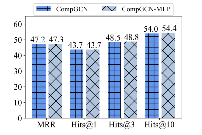
(a) WN18RR

Figure 3: KGC results of CompGCN and CompGCN-MLP on WN18RR. On this dataset, CompGCN-MLP achieves compare performance as CompGCN.

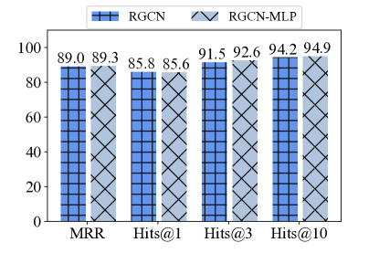
(a) WN18

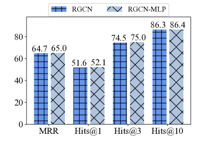
(b) FB15K

Figure 4: KGC results of RGCN and RGCN-MLP on FB15K and WN18. On all three datasets, RGCN-MLP achieves comparable performance as RGCN.

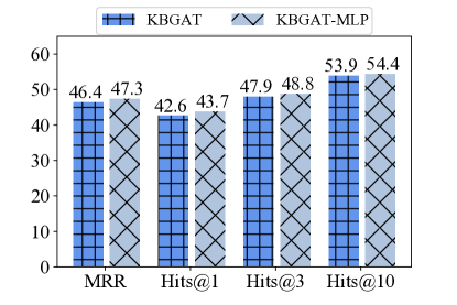
(a) WN18RR

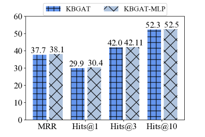
(b) NELL-995

Figure 5: KGC results of KBGAT and KBGAT-MLP on WN18RR and NELL-995. On all three datasets, KBGAT-MLP achieves comparable performance as KBGAT.

In section 3.1, We replace the message passing with the MLP while keeping other components untouched in CompGCN, RGCN and KBGAT. Due to the space limit, we only present the resutls on the FB15K-237 dataset in section 3.1. In this section, we include additional results on other datasets. Specifically, we include results of CompGCN/CompGCN-MLP on the WN18RR dataset, RGCN/RGCN-MLP on the WN18 and FB15K dataset, KBGAT/KBGAT-MLP on the WN18RR and NELL-995 in Figure 3, Figure 4 and Figure 5 respectively. All the counterpart MLP-based models achieve similar performance with the corresponding MPNN-based models, which show similar observations with the FB15K-237 datasets in section 3.1.

Appendix G MPNNs with random graph structure for message passing

In this section, we investigate how the performance perform when we use random generated graph structure in the message passing process. The number of random edges is the same as the ones in the original graph. When training the model by optimizing the loss function, we still use the original graph structure, i.e., $\mathcal{D}^{*}_{train}$ in Eq. (7) is fixed in Appendix E. Note that if the message passing has some contribution to the performance, aggregating the random edges should lead to the performance drop.

We present the results of CompGCN, RGCN and KBGAT on various datasets in Table 7. We use “Original", “Random" to denote the performance with the original graph structure and random edges respectively. From Table 7, we observe that using the noise edges achieves comparable performance, which further indicates that the message passing component is not the key part.

Appendix H Time Complexity

We first define the sizes of weight matrices and embeddings of a single layer. We denote the dimension of entity and relation embeddings as $d$. The weight matrices in RGCN and CompGCN (shown in Eqs. (1) and (2) respectively in Appendix C. ) are $d\times d$ matrices. In KBGAT (Eq. (3) in Appendix C), there are two weight matrices $\mathbf{W}_{1}$ and $\mathbf{W}_{2}$ of size $d\times 3d$ and $1\times d$, respectively. Thus, the time complexity of RGCN, CompGCN, KBGAT for a single layer is $O(|E|d^{2}+nd^{2})$, $O(|E|d^{2}+nd^{2})$, $O(3|E|d^{2}+nd^{2}+|E|d)$, respectively, where $|E|$ is the number of edges and $n$ is the number of nodes. While MLP doesn’t have the message passing operation, the time complexity in a single layer is $O(nd^{2})$. Note $|E|$ is usually much larger than $n$, thus the MLP is more efficient than MPNN.

Appendix I Ensembling MLPs

We briefly introduce the MLP-based models we utilized for constructing the ensemble model in section 4.2 for the three datasets as follows:

• For the FB15K-237 dataset, we ensemble the following models: DistMult + w/o sampling; DistMult + with sampling (two different settings with the number of negative samples as $0.5N$ and $N$, respectively); ConvE + w/o sampling; ConvE + with sampling (five different settings with the number of negative samples as $50,200,500,$ $0.5N$ and $N$, respectively).

• For the WN18RR dataset, we ensemble the following models: DistMult + w/o sampling; ConvE+ w/o sampling; ConvE+ with sampling (one setting with the number of negative samples as $N$).

• For the NELL-995 dataset, we ensemble the following models: ConvE+ w/o sampling; ConvE+with sampling (five settings with the number of negative samples as $50,200,500,0.5N$ and $N$).

References

- Bollacker et al. (2008) Kurt Bollacker, Colin Evans, Praveen Paritosh, Tim Sturge, and Jamie Taylor. 2008. Freebase: a collaboratively created graph database for structuring human knowledge. In Proceedings of the 2008 ACM SIGMOD international conference on Management of data, pages 1247–1250.
- Bordes et al. (2013) Antoine Bordes, Nicolas Usunier, Alberto García-Durán, Jason Weston, and Oksana Yakhnenko. 2013. Translating embeddings for modeling multi-relational data. In Advances in Neural Information Processing Systems 26: 27th Annual Conference on Neural Information Processing Systems 2013. Proceedings of a meeting held December 5-8, 2013, Lake Tahoe, Nevada, United States, pages 2787–2795.
- Carlson et al. (2010) Andrew Carlson, Justin Betteridge, Bryan Kisiel, Burr Settles, Estevam R Hruschka, and Tom M Mitchell. 2010. Toward an architecture for never-ending language learning. In Twenty-Fourth AAAI conference on artificial intelligence.
- Dettmers et al. (2018) Tim Dettmers, Pasquale Minervini, Pontus Stenetorp, and Sebastian Riedel. 2018. Convolutional 2d knowledge graph embeddings. In Proceedings of the Thirty-Second AAAI Conference on Artificial Intelligence, (AAAI-18), the 30th innovative Applications of Artificial Intelligence (IAAI-18), and the 8th AAAI Symposium on Educational Advances in Artificial Intelligence (EAAI-18), New Orleans, Louisiana, USA, February 2-7, 2018, pages 1811–1818. AAAI Press.
- Fan et al. (2019) Wenqi Fan, Yao Ma, Qing Li, Yuan He, Eric Zhao, Jiliang Tang, and Dawei Yin. 2019. Graph neural networks for social recommendation. In The World Wide Web Conference, pages 417–426.
- Fellbaum (2010) Christiane Fellbaum. 2010. Wordnet. In Theory and applications of ontology: computer applications, pages 231–243. Springer.
- García-Durán et al. (2018) Alberto García-Durán, Sebastijan Dumančić, and Mathias Niepert. 2018. Learning sequence encoders for temporal knowledge graph completion. arXiv preprint arXiv:1809.03202.
- Jin et al. (2021) Wei Jin, Lingxiao Zhao, Shichang Zhang, Yozen Liu, Jiliang Tang, and Neil Shah. 2021. Graph condensation for graph neural networks. arXiv preprint arXiv:2110.07580.
- Jin et al. (2019) Woojeong Jin, Meng Qu, Xisen Jin, and Xiang Ren. 2019. Recurrent event network: Autoregressive structure inference over temporal knowledge graphs. arXiv preprint arXiv:1904.05530.
- Lin et al. (2015) Yankai Lin, Zhiyuan Liu, Maosong Sun, Yang Liu, and Xuan Zhu. 2015. Learning entity and relation embeddings for knowledge graph completion. In Twenty-ninth AAAI conference on artificial intelligence.
- Liu et al. (2021) Hanxiao Liu, Zihang Dai, David R So, and Quoc V Le. 2021. Pay attention to mlps. arXiv preprint arXiv:2105.08050.
- Ma et al. (2021) Yao Ma, Xiaorui Liu, Tong Zhao, Yozen Liu, Jiliang Tang, and Neil Shah. 2021. A unified view on graph neural networks as graph signal denoising. In Proceedings of the 30th ACM International Conference on Information & Knowledge Management, pages 1202–1211.
- Nathani et al. (2019) Deepak Nathani, Jatin Chauhan, Charu Sharma, and Manohar Kaul. 2019. Learning attention-based embeddings for relation prediction in knowledge graphs. In Proceedings of the 57th Annual Meeting of the Association for Computational Linguistics, pages 4710–4723.
- Schlichtkrull et al. (2018) Michael Schlichtkrull, Thomas N Kipf, Peter Bloem, Rianne Van Den Berg, Ivan Titov, and Max Welling. 2018. Modeling relational data with graph convolutional networks. In European semantic web conference, pages 593–607. Springer.
- Sun et al. (2020) Zhiqing Sun, Shikhar Vashishth, Soumya Sanyal, Partha Talukdar, and Yiming Yang. 2020. A re-evaluation of knowledge graph completion methods. In Proceedings of the 58th Annual Meeting of the Association for Computational Linguistics, pages 5516–5522.
- Tolstikhin et al. (2021) Ilya Tolstikhin, Neil Houlsby, Alexander Kolesnikov, Lucas Beyer, Xiaohua Zhai, Thomas Unterthiner, Jessica Yung, Daniel Keysers, Jakob Uszkoreit, Mario Lucic, et al. 2021. Mlp-mixer: An all-mlp architecture for vision. arXiv preprint arXiv:2105.01601.
- Toutanova and Chen (2015) Kristina Toutanova and Danqi Chen. 2015. Observed versus latent features for knowledge base and text inference. In Proceedings of the 3rd workshop on continuous vector space models and their compositionality, pages 57–66.
- Toutanova et al. (2015) Kristina Toutanova, Danqi Chen, Patrick Pantel, Hoifung Poon, Pallavi Choudhury, and Michael Gamon. 2015. Representing text for joint embedding of text and knowledge bases. In Proceedings of the 2015 conference on empirical methods in natural language processing, pages 1499–1509.
- Vashishth et al. (2020) Shikhar Vashishth, Soumya Sanyal, Vikram Nitin, and Partha P. Talukdar. 2020. Composition-based multi-relational graph convolutional networks. In 8th International Conference on Learning Representations, ICLR 2020, Addis Ababa, Ethiopia, April 26-30, 2020. OpenReview.net.
- Wang et al. (2019) Xiang Wang, Xiangnan He, Yixin Cao, Meng Liu, and Tat-Seng Chua. 2019. Kgat: Knowledge graph attention network for recommendation. In Proceedings of the 25th ACM SIGKDD International Conference on Knowledge Discovery & Data Mining, pages 950–958.
- West et al. (2014) Robert West, Evgeniy Gabrilovich, Kevin Murphy, Shaohua Sun, Rahul Gupta, and Dekang Lin. 2014. Knowledge base completion via search-based question answering. In Proceedings of the 23rd international conference on World wide web, pages 515–526.
- Xiong et al. (2017a) Chenyan Xiong, Russell Power, and Jamie Callan. 2017a. Explicit semantic ranking for academic search via knowledge graph embedding. In Proceedings of the 26th international conference on world wide web, pages 1271–1279.
- Xiong et al. (2017b) Wenhan Xiong, Thien Hoang, and William Yang Wang. 2017b. Deeppath: A reinforcement learning method for knowledge graph reasoning. In Proceedings of the 2017 Conference on Empirical Methods in Natural Language Processing, EMNLP 2017, Copenhagen, Denmark, September 9-11, 2017, pages 564–573. Association for Computational Linguistics.
- Yang et al. (2015) Bishan Yang, Wen-tau Yih, Xiaodong He, Jianfeng Gao, and Li Deng. 2015. Embedding entities and relations for learning and inference in knowledge bases. In 3rd International Conference on Learning Representations, ICLR 2015, San Diego, CA, USA, May 7-9, 2015, Conference Track Proceedings.
- Ye et al. (2019) Rui Ye, Xin Li, Yujie Fang, Hongyu Zang, and Mingzhong Wang. 2019. A vectorized relational graph convolutional network for multi-relational network alignment. In IJCAI, pages 4135–4141.
- Ying et al. (2018) Rex Ying, Ruining He, Kaifeng Chen, Pong Eksombatchai, William L Hamilton, and Jure Leskovec. 2018. Graph convolutional neural networks for web-scale recommender systems. In Proceedings of the 24th ACM SIGKDD International Conference on Knowledge Discovery & Data Mining, pages 974–983.
- Yu et al. (2021) Donghan Yu, Yiming Yang, Ruohong Zhang, and Yuexin Wu. 2021. Knowledge embedding based graph convolutional network. In Proceedings of the Web Conference 2021, pages 1619–1628.
- Zhang et al. (2022a) Shichang Zhang, Yozen Liu, Yizhou Sun, and Neil Shah. 2022a. Graph-less neural networks: Teaching old mlps new tricks via distillation. ICLR.
- Zhang and Yao (2022) Yongqi Zhang and Quanming Yao. 2022. Knowledge graph reasoning with relational digraph. In Proceedings of the ACM Web Conference 2022, pages 912–924.
- Zhang et al. (2022b) Zhanqiu Zhang, Jie Wang, Jieping Ye, and Feng Wu. 2022b. Rethinking graph convolutional networks in knowledge graph completion. In Proceedings of the ACM Web Conference 2022, pages 798–807.
- Zhao et al. (2022) Lingxiao Zhao, Wei Jin, Leman Akoglu, and Neil Shah. 2022. From stars to subgraphs: Uplifting any gnn with local structure awareness. ICLR.
- Zhu et al. (2022) Zhaocheng Zhu, Xinyu Yuan, Louis-Pascal Xhonneux, Ming Zhang, Maxime Gazeau, and Jian Tang. 2022. Learning to efficiently propagate for reasoning on knowledge graphs. arXiv preprint arXiv:2206.04798.
- Zhu et al. (2021) Zhaocheng Zhu, Zuobai Zhang, Louis-Pascal Xhonneux, and Jian Tang. 2021. Neural bellman-ford networks: A general graph neural network framework for link prediction. Advances in Neural Information Processing Systems, 34.
- Zoph and Le (2016) Barret Zoph and Quoc V Le. 2016. Neural architecture search with reinforcement learning. arXiv preprint arXiv:1611.01578.