DProQ: A Gated-Graph Transformer for Protein Complex Structure Assessment

Abstract

Proteins interact to form complexes to carry out essential biological functions. Computational methods have been developed to predict the structures of protein complexes. However, an important challenge in protein complex structure prediction is to estimate the quality of predicted protein complex structures without any knowledge of the corresponding native structures. Such estimations can then be used to select high-quality predicted complex structures to facilitate biomedical research such as protein function analysis and drug discovery. We challenge this significant task with DProQ, which introduces a gated neighborhood-modulating Graph Transformer (GGT) designed to predict the quality of 3D protein complex structures. Notably, we incorporate node and edge gates within a novel Graph Transformer framework to control information flow during graph message passing. We train and evaluate DProQ on four newly-developed datasets that we make publicly available in this work. Our rigorous experiments demonstrate that DProQ achieves state-of-the-art performance in ranking protein complex structures.

1 Introduction

Proteins, bio-molecules, or biological macro-molecules perform a broad range of functions in modern biology and bioinformatics. Protein-protein interactions (PPI) play a key role in almost all biological processes. Understanding the mechanisms and functions of PPI may benefit studies in other scientific areas such as drug discovery [1, 2, 3] and protein design [4, 5, 6]. Typically, high-resolution 3D structures of protein complexes can be determined using experimental solutions (e.g., X-ray crystallography and cryo-electron microscopy). However, due to the high financial and resource-intensive costs associated with them, these methods are not satisfactory for the increasing demands in modern biology research. In the context of this practical challenge, computational methods for protein complex structure prediction have recently been receiving an increasing amount of attention.

Recently, the ab initio method AlphaFold-Multimer [7] released an end-to-end system for protein complex structure prediction. The system improves its prediction accuracy on multimeric proteins considerably. However, compared to AlphaFold2’s outstanding performance in monomer structure prediction [8], the accuracy level for protein quaternary structure prediction still has much room for progress. Within this context, estimation of model accuracy methods (EMA) and quality assessment methods (QA) play a significant role in the advancement of protein complex structure prediction [9].

However, existing EMA methods have two primary shortcomings. The first is that they have not explored the use of Transformer-like architectures [10] to enhance the expressiveness of neural networks designed for structure quality assessment. The second shortcoming is that current training or benchmark datasets for QA [11, 12, 13] cannot fully represent the accuracy level of the latest protein complex structure predictors [14, 8, 15]. Most of the latest QA datasets were generated using classical tools [16, 17] and, as such, typically contain only a few near-native decoys for each protein target. Consequently, EMA methods trained using these classical datasets may not be complementary to high-accuracy protein complex structure predictors.

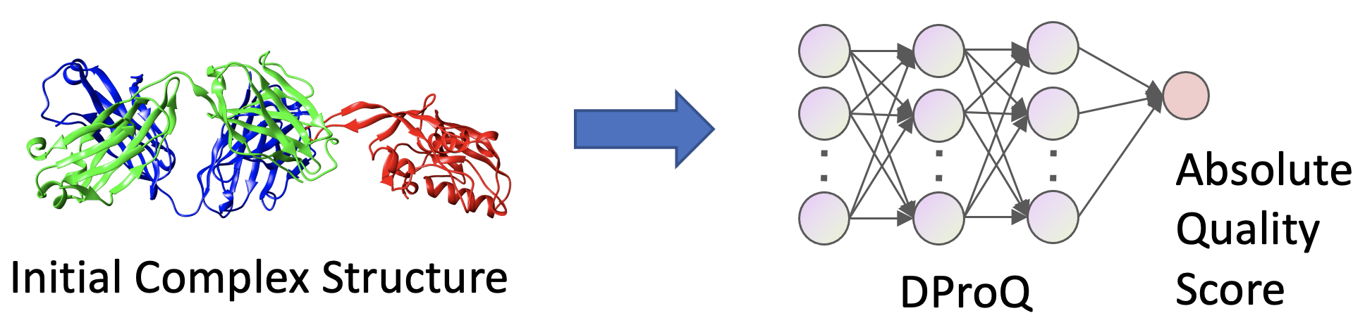
Figure 1: An overview of the protein structure quality assessment problem addressed by DProQ.

Here, we introduce the Deep Protein Quality (DProQ) for structural ranking of protein complexes - Figure 1. In particular, DProQ introduces the Gated Graph Transformer, a novel graph neural network (GNN) that learns to modulate its input information to better guide its structure quality predictions. Being that DProQ requires only a single forward pass to finalize its predictions, we achieve prediction time speed-ups compared to existing QA solutions. Moreover, our model poses structure quality assessment as a multi-task problem, making it the first of its kind in deep learning (DL)-based structure assessment.

2 Related Work

We now proceed to describe prior works relevant to DL-based structure quality assessment.

Biomolecular structure prediction. Predicting biomolecular structures has been an essential problem for the last several decades. However, very recently, the problem of protein tertiary structure prediction has largely been solved by new DL methods [8, 18]. Furthermore, [15] and others have begun making advancements in protein complex structure prediction. Such structure prediction methods have notably accelerated the process of determining 3D protein structures. As such, modern DL-based structure predictors have benefited many related research areas such as drug discovery [3] and protein design [19].

Protein representation learning. Protein structures can be represented in various ways. Previously, proteins have been represented as tableau data in the form of hand-crafted features [20]. Along this line, many works [21, 22] have represented proteins using pairwise information embeddings such as residue-residue distance maps and contact maps. Recently, describing proteins as graphs has become a popular means of representing proteins, as such representations can learn and leverage proteins’ geometric information more naturally. For example, EnQA [23] used equivariant graph representations to estimate the per-residue quality of protein structures. Moreover, the Equivariant Graph Refiner (EGR) model formulated structural refinement and assessment of protein complexes using semi-supervised equivariant graph neural networks.

Expert techniques for protein structure quality assessment. Over the past few decades, many EMA methods have been developed to solve the challenging task of QA [24, 25, 26, 27, 28]. Among these scoring methods, machine learning-based EMA methods have shown better performance than physics-based [29, 30] and statistics-based methods [31, 32].

Machine learning for protein structure quality assessment. Newly-released machine learning methods have utilized various techniques and features to approach the task of structural QA. For example, ProQDock [27] and iScore [28] used protein structure data as the input for a support vector machine classifier. Similarly, EGCN [33] assembled graph pairs to represent protein-protein structures and then employed a graph convolutional network (GCN) to learn graph structural information. DOVE [34] used a 3D convolutional neural network (CNN) to describe protein-protein interfaces as input features. In a similar spirit, GNN_DOVE [35] and PPDocking [36] trained Graph Attention Networks [37] to evaluate protein complex decoys. Moreover, PAUL [38] used a rotation-equivariant neural network to identify accurate models of protein complexes at an atomic level.

Deep representation learning with Transformers. Increasingly more works have applied in different domains Transformer-like architectures or multi-head attention (MHA) mechanisms to achieve state-of-the-art (SOTA) results. For example, the Swin-Transformer achieved SOTA performance in various computer vision tasks [39, 40, 41]. Likewise, the MSA Transformer [42] used tied row and column MHA to address many important tasks in computational biology. Moreover, DeepInteract[43] introduced the Geometric Transformer to model protein chains as graphs for protein interface contact prediction.

Contributions. Our work builds upon prior works by making the following contributions:

1. We present the new DProQ pipeline, trained using our newly-developed protein complex datasets in which all structural decoys were generated using AlphaFold2 [8] and AlphaFold-Multimer [7].

2. Using our newly-developed Heterodimer-AF2 (HAF2) and Docking Benchmark 5.5-AF2 (DMB55-AF2) datasets, we demonstrate the superiority of DProQ compared to GNN_DOVE, the current state-of-the-art for structural QA of protein complexes.

3. We provide the first example of applying Transformer representation learning to the task of protein structure quality assessment, by introducing the new Gated Graph Transformer architecture to iteratively update node and edge representations using adaptive feature modulation.

3 DProQ Pipeline

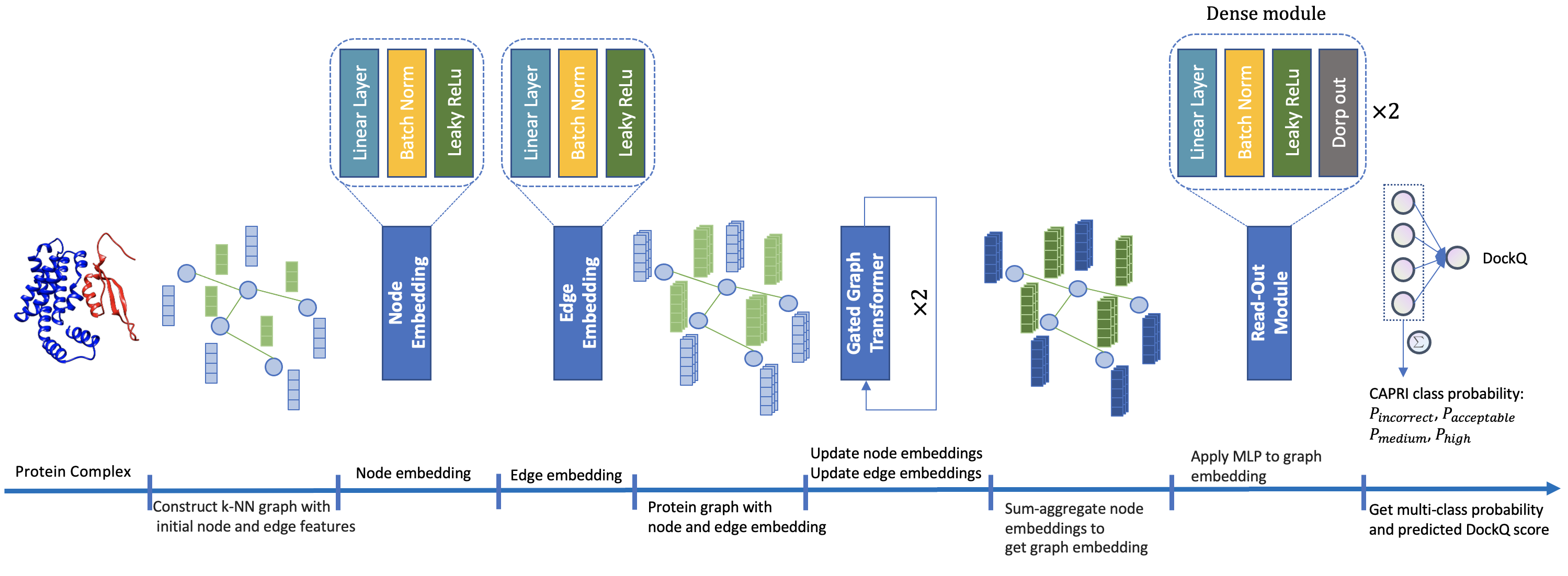
Figure 2: An overview of the DProQ pipeline for quality assessment of protein complexes.

We will now begin to describe DProQ. Shown in Figure 1 and illustrated from from left to right in Figure 2, DProQ first receives a 3D protein complex structure as input and represents it as a spatial graph. Notably, all chains in the complex are represented within the same graph topology, where connected pairs of atoms from the same chain are distinguished using a binary edge feature, as described in the following sections. DProQ models protein complexes in this manner to facilitate explicit information flow between chains, which has proven useful for other tasks on macromolecular structures [44, 45]. We note that DProQ is not trained using any coevolutionary features, making it an end-to-end geometric deep learning method for protein complex structures.

K-NN graph representation. DProQ represents each input protein complex structure as a spatial k-nearest neighbors (k-NN) graph $\mathcal{G}=(\mathcal{V},\mathcal{E})$, where the protein’s C$\alpha$ atoms serve as $\mathcal{V}$ (i.e., the nodes of $\mathcal{G}$). After constructing $\mathcal{G}$ by connecting each node to its 10 closest neighbors in $\mathbb{R}^{3}$, we denote its initial node features as $\mathbf{F}\in\mathbb{R}^{d\times N}$ (e.g., residue type) and its initial edge features as $\mathbf{E}\in\mathbb{R}^{d\times M}$ (e.g., C$\alpha$-C$\alpha$ distance), as described more thoroughly in Appendix B.

Node and edge embeddings. After receiving a protein complex graph $\mathcal{G}$ as input, DProQ applies initial node and edge embedding modules to each node and edge, respectively. We define such embedding modules as $Embed(\mathbf{F})=\varphi^{h}(\mathbf{f}_{i}),\forall(i)\in\mathcal{V}$ and $Embed(\mathbf{E})=\varphi^{e}(\mathbf{f}_{j\rightarrow i}),\forall(i,j)\in\mathcal{E}$, respectively, where each $\varphi$ function is represented as a shallow neural network consisting of a linear layer, batch normalization, and LeakyReLU activation [46]. Such node and edge embeddings are then fed as an updated input graph into the new Gated Graph Transformer.

3.1 Gated Graph Transformer architecture

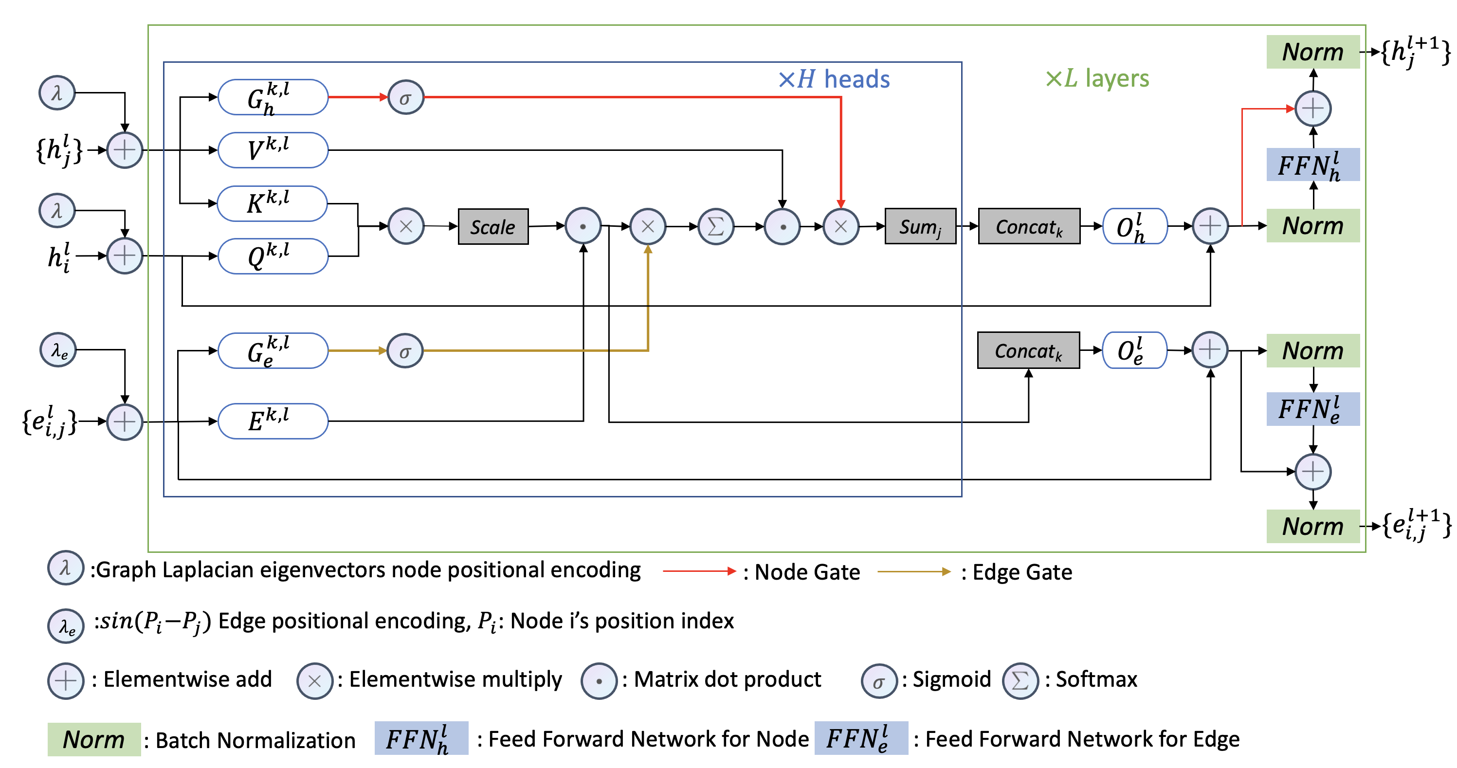
Figure 3: GGT model architecture.

We designed the Gated Graph Transformer (GGT) as a solution to a specific phenomenon in graph representation learning. Note that, unlike other GNN-based structure scoring methods, [35, 36] define edges using a fixed distance threshold, which means that each graph node may have a different number of incoming and outgoing edges. In contrast, DProQ constructs and operates on k-NN graphs where all nodes are connected to the same number of neighbors. However, in the context of k-NN graphs, each neighbor’s information is, by default, given equal priority during information updates. As such, we may desire to imbue our graph neural network with the ability to automatically decide the priority of different nodes and edges during the graph message passing. Consequently, we present the GGT, a gated neighborhood-modulating Graph Transformer inspired by [37, 47, 43]. Formally, to update the network’s node embeddings $\mathbf{h}_{i}$ and edge embeddings $\mathbf{e}_{ij}$, we define a single layer of the GGT as:

$$\widehat{\widehat{\mathbf{w}}}_{ij}^{k,\ell}=\left(\frac{Q^{k,\ell}\mathbf{h}_{i}^{\ell}\cdot K^{k,\ell}\mathbf{h}_{j}^{\ell}}{\sqrt{d_{k}}}\right)\cdot E^{k,\ell}\mathbf{e}_{ij}^{\ell}$$ (1)

$$\hat{\mathbf{e}}_{ij}^{\ell+1}=\mathbf{O}_{e}^{\ell}\|_{k=1}^{H}\left(\widehat{\widehat{\mathbf{w}}}_{ij}^{k,\ell}\right)$$ (2)

$$\widehat{\mathbf{w}}_{ij}^{k,\ell}=\widehat{\widehat{\mathbf{w}}}_{ij}^{k,\ell}\times\operatorname{sigmoid}\left(\mathbf{G}_{e}^{k,\ell}\mathbf{e}_{ij}^{\ell}\right)$$ (3)

$$\mathbf{w}_{ij}^{k,\ell}=\operatorname{softmax}\left(\hat{\mathbf{w}}_{ij}^{k,\ell}\right)$$ (4)

$$\hat{\mathbf{h}}_{i}^{\ell+1}=O_{\mathbf{h}}^{\ell}\|_{k=1}^{H}\left(\operatorname{sigmoid}\left(G_{h}^{k,\ell}\mathbf{h}_{j}^{\ell}\right)\times\sum_{j\in\mathcal{N}_{i}}\mathbf{w}_{ij}^{k,\ell}V^{k,\ell}\mathbf{h}_{j}^{\ell}\right)$$ (5)

In particular, the GGT introduces to the standard Graph Transformer architecture [47] two information gates through which the network can modulate node and edge information flow, as shown in Figure 3. Equation 2 shows how the output of the edge gate, $\mathbf{G}_{e}$, is used elementwise to gate the network’s attention scores $\widehat{\widehat{\mathbf{w}}}_{ij}$ derived from Equation 1. Such gating simultaneously allows the network to decide how much to regulate edge information flow as well as how much to weigh the edge of each node neighbor. Similarly, the node gate, $\mathbf{G}_{h}$, shown in Equation 5, allows the GGT to individually decide how to modulate information from node neighbors during node information updates. Lastly, for the GGT’s Feed Forward Network, we keep the same structure as described in [47], providing us with new node embeddings $\hat{\mathbf{h}}_{i}^{L}$ and edge embeddings $\hat{\mathbf{e}}_{ij}^{L}$. For additional background on the GGT’s network operations, we refer readers to [47].

3.2 Multi-task graph property prediction

To obtain graph-level predictions for each input protein complex graph, we apply a graph sum-pooling operator on $\hat{\mathbf{h}}_{i}^{L}$ such that $\mathbf{p}\in\mathbb{R}^{d\times 1}=\sum_{i=1}^{N}\mathbf{h}_{i}^{L}$. This graph embedding $\mathbf{p}$ is then fed as input to DProQ’s first read-out module $\varphi_{1}^{r}$, where each read-out module consists of a series of linear layers, batch normalization layers, LeakyReLU activations, and dropout layers [48], respectively. That is, $\mathbf{\hat{p}}\in\mathbb{R}^{d\times 4}=\varphi_{1}^{r}(\mathbf{p})$ reduces the dimensionality of $\mathbf{p}$ to accommodate DProQ’s output head designed for graph classification. Specifically, for graph classification, we apply a Softmax layer such that $\mathbf{y}\in\mathbb{R}^{d\times 4}=softmax(\mathbf{\hat{p}})$, where $\mathbf{y}$ is the network’s predicted DockQ structure quality class probabilities [49] for each input protein complex (e.g., Medium, High). Thereafter, we apply DProQ’s second read-out module $\varphi_{2}^{r}$ to $\mathbf{\hat{p}}$ such that $\mathbf{q}\in\mathbb{R}^{1\times 1}=\varphi_{2}^{r}(\mathbf{\hat{p}})$. Within this context, the network’s scalar graph regression output $\mathbf{q}$ represents the network’s predicted DockQ score [49] for a given protein complex input.

Structure quality scoring loss. To train DProQ’s graph regression head, we used the mean squared error loss $\mathcal{L}_{R}=\frac{1}{N}\sum_{i=1}^{N}\|\mathbf{q}_{i}^{\prime}-\mathbf{q}_{i}^{*}\|^{2}$. Here, $\mathbf{q}_{i}^{\prime}$ is the model’s predicted DockQ score for example $i$, $\mathbf{q}_{i}^{*}$ is the ground truth DockQ score for example $i$, and $N$ represents the number of examples in a given mini-batch.

Structure quality classification loss. Likewise, to train DProQ’s graph classification head, we used the cross-entropy loss $\mathcal{L}_{C}=\frac{1}{N}\sum_{i=1}^{N}\left(\mathbf{y}_{i}^{*}-\log(\mathbf{y}_{i}^{\prime})\right)$. Here, $\mathbf{y}_{i}^{\prime}$ is the model’s predicted DockQ quality class (e.g., Acceptable) for example $i$, and $\mathbf{y}_{i}^{*}$ is the ground truth DockQ quality class (e.g., Incorrect) for example $i$.

Overall loss. We define DProQ’s overall loss as $\mathcal{L}=w_{\mathcal{L}_{C}}\times\mathcal{L}_{C}+w_{\mathcal{L}_{R}}\times\mathcal{L}_{R}$. We note that the weights for each constituent loss (e.g., $w_{\mathcal{L}_{R}}$) were determined either by performing a grid search or instead by using a lowest validation loss criterion for parameter selection. In Appendix C, we describe DProQ’s choice of hyperparameters in greater detail.

4 Experiments

4.1 Data

Here, we briefly describe our four new datasets for complex structural QA, datasets that we used to train, validate, and test all DProQ models. Appendix B describes in greater detail how we generated these datasets as well as their corresponding labels .

Dataset Labels. As shown in Section 3.2, DProQ performs two learning tasks simultaneously. In the framework of its graph regression task, DProQ treats DockQ scores [49] as its per-graph labels. As introduced earlier, DockQ scores are robust, continuous values in the range of [0, 1]. Such scores measure the quality of a protein complex structure such that a higher DockQ score indicates a higher-quality structure. In the context of its graph classification task, DProQ predicts the probabilities that the structure of an input protein complex falls into the Incorrect, Acceptable, Medium, or High-quality category, where assignments into such quality categories are made according to the structure’s true DockQ score.

Multimer-AF2 Dataset. To build our first new training and validation dataset, the Multimer-AF2 (MAF2) dataset, we used AlphaFold 2 [8] and AlphaFold-Multimer [7] to generate protein complex structures for protein targets derived from the EVCoupling [50] and DeepHomo [51] datasets. In summary, the MAF2 dataset contains a total of $9,251$ decoys, where according to DockQ scores $20.44\%$ of them are of Incorrect quality, $14.34\%$ of them are of Acceptable quality, $30.00\%$ of them are of Medium quality, and the remaining $35.22\%$ of them are of High quality.

Docking Decoy Set. Our second new training and validation dataset, the Docking Decoy dataset [52], contains $58$ protein complex targets. Each target includes approximately $100$ Incorrect decoys and at least one near-native decoy. To construct this dataset, we follow the sequence clustering results from GNN_DOVE [35], select as an optional testing dataset the fourth clustering fold consisting of $14$ targets, and use the remaining $3$ folds for training and validation, where such training and validation splits consist of $34$ targets and $10$ targets, respectively.

Heterodimer-AF2 Dataset. We built our first new test dataset, the Heterodimer-AF2 (HAF2) dataset, by collecting the structures of heterodimers from the Protein Data Bank [53]. Thereafter, we used a custom, in-house AlphaFold-Multimer [7] system to generate different models for each protein heterodimer, subsequently applying 40% sequence identity filtering to each split for this dataset. Overall, the HAF2 dataset consists of a total of $13$ targets containing $1,849$ decoys, where $33.36\%$ of these decoys are of Incorrect quality, $6.13\%$ of them are of Acceptable quality, $35.62\%$ of them are of Medium quality, and the remaining $24.58\%$ of them are of High quality.

Docking Benchmark5.5 AF2 Dataset. To construct our final test dataset, the Docking Benchmark 5.5-AF2 (DBM55-AF2) dataset, we applied AlphaFold-Multimer [7] to predict the structures of Docking Benchmark 5.5 targets [54]. This dataset contains a total of $15$ protein targets comprised of $449$ decoys. $50.78\%$ of these decoys are of Incorrect quality, $16.70\%$ of them are of Acceptable quality, $30.73\%$ of them are of Medium quality, and the remaining $1.78\%$ of them are of High quality.

Cross-Validation Datasets and Overlap Reduction. All DProQ models were trained on $8,733$ decoys and validated on $3,407$ decoys derived as a combination of our MAF2 and Docking Decoy datasets. After training, each model was blindly tested on our HAF2 and DBM55-AF2 test datasets. To prevent data leakage between our training and test datasets, we used MMseqs2 [55] to perform $30\%$ sequence identity filtering w.r.t. our test dataset and training dataset splits. After filtering, we further remove any targets that do not contain any Acceptable or higher-quality decoys according to DockQ’s score classifications [49].

4.2 Evaluation Setup

Baselines. We compare our method with the state-of-the-art method GNN_DOVE, an atom-level graph attention-based method for protein complex structure evaluation. Uniquely, it extracts protein interface areas to build its input graphs. Further, the chemical properties of its atoms as well as inter-atom distances are treated as initial node and edge features, respectively. We note that GNN_DOVE is the sole baseline we include in this study, as for all other DL-based methods for structural QA, we were unable to locate reproducible training and inference code for such methods. Furthermore, since GNN_DOVE has previously been evaluated against several other classical machine learning methods for structural QA and has demonstrated strong performance against such methods, we argue that comparing new DL methods’ performance to GNN_DOVE can serve as a strong indicator of the DL state-of-the-art for the field.

DProQ Models. Besides including results for the standard DProQ model as well as for GNN_DOVE, we also report results on the HAF2 and DBM55-AF2 datasets for a selection of DProQ variants curated in this study. The DProQ variants we chose to investigate in this work include DProQ_GT which employs the original Graph Transformer architecture [47]; DProQ_GTE which employs the GGT with only its edge gate enabled; and DProQ_GTN which employs the GGT with only its node gate enabled.

Evaluation metrics. We evaluate structural QA performance according to two main criteria. Our first criterion is general ranking ability which measures how many qualified decoys are found within a model’s predicted Top-$N$ structure ranking. Within this framework, a model’s hit rate is defined as the fraction of protein complex targets for which the model, within each of its Top-$N$ ranks, ranked at least one Acceptable or higher-quality decoy based on the CAPRI scoring criteria [12]. In this work, we report results based on models’ Top-10 hit rates. A hit rate is represented by three numbers separated by the character /. These three numbers, in order, represent how many decoys with Acceptable or higher-quality, Medium or higher-quality, and High quality were among the Top-N ranked decoys. Our second criterion with which to score models is their Top-$1$ selected model ranking ability. Within this context, we calculate the ranking loss for each method. Here, per-target ranking loss is defined as the difference between the DockQ score of a target’s native structure and the DockQ score of the top decoy predicted by each ranking method. As such, a lower ranking loss indicates a stronger model for ranking pools of structural decoys for downstream tasks.

Implementation Details. We train all our models using the AdamW optimizer [56] and perform early stopping with a patience of $15$ epochs. All remaining hyperparameters and graph features we used are described further in Appendix C. Source code to reproduce our results and perform fast structure quality assessment using our model weights can be found at https://github.com/BioinfoMachineLearning/DProQ.

4.3 Results

Blind Structure Quality Assessment on the HAF2 Dataset. Table 1 reports the hit rate performances of DProQ, DProQ variants, and GNN_DOVE, respectively, on the HAF2 Dataset. On $13$ HAF2 targets, DProQ hits (i.e., identifies at least one suitable decoy structure for) $10$ targets on the Acceptable quality level, $9$ targets on the Medium quality level, and $4$ targets on High quality level. For targets with High quality structures, DProQ and its variants successfully hit all of them. On the HAF2 dataset, GNN_DOVE gets a $8/7/3$ hit rate on Acceptable, Medium, and High quality targets respectively. However, DProQ outperforms GNN_DOVE on all targets except 7NKZ. On this target, GNN_DOVE achieves a better hit rate on High quality decoy structures. Overall, DProQ shows a better performance than DProQ_GT, DProQ_GTE, and DProQ_GTN. Additionally, for target 7MRW, only DProQ successfully hits the $5$ Acceptable quality targets and $4$ Medium quality targets, whereas all other methods failed to hit any qualified decoy structures for this protein target.

Table 2 reports methods’ ranking loss performance on each HAF2 target. DProQ and its $3$ variants outperform GNN_DOVE which displays the highest average ranking loss. In particular, DProQ achieves the lowest average ranking loss of $0.195$ compared to all other methods. Here, DProQ’s loss is $43\%$ lower than GNN_DOVE’s $0.343$ average ranking loss. Moreover, DProQ achieves the lowest loss on $5$ targets, namely 7AWV, 7OEL, 7NRW, 7NKZ and 7O27. Notably, DProQ_GT, DProQ_GTE, and DProQ_GTN’s ranking losses here are $29\%$, $34\%$, and $30\%$ lower, respectively, than GNN_DOVE’s average ranking loss.

Table 1: Hit rate performance on the HAF2 dataset. The Best column represents each target’s best-possible Top-$10$ result. The Summary row lists the results when all targets are taken into consideration.

ID	DProQ	DProQ_GT	DProQ_GTE	DProQ_GTN	GNN_DOVE	BEST
7AOH	10/10/10	10/10/10	10/10/10	10/10/10	9/9/0	10/10/10
7D7F	0/0/0	0/0/0	0/0/0	0/0/0	0/0/0	5/0/0
7AMV	10/10/10	10/10/10	10/10/10	10/10/10	10/10/6	10/10/10
7OEL	10/10/0	10/9/0	10/10/0	10/10/0	10/10/0	10/10/0
7O28	10/10/0	10/10/0	10/10/0	10/10/0	10/10/0	10/10/0
7ALA	0/0/0	0/0/0	0/0/0	0/0/0	0/0/0	1/0/0
7MRW	5/4/0	0/0/0	0/0/0	0/0/0	0/0/0	10/10/0
7OZN	0/0/0	0/0/0	0/0/0	0/0/0	0/0/0	10/2/0
7D3Y	2/0/0	5/0/0	6/0/0	8/0/0	0/0/0	10/0/0
7NKZ	10/10/2	10/10/1	10/10/1	10/010/4	10/9/9	10/10/10
7LXT	1/1/0	0/0/0	0/0/0	0/0/0	1/0/0	10/10/0
7KBR	10/10/10	10/10/10	10/10/10	10/10/10	10/10/9	10/10/10
7O27	10/10/0	10/10/0	10/10/0	10/10/0	10/4/0	10/10/0
Summary	10/9/4	8/7/4	8/7/4	8/7/4	8/7/3	13/10/4

Table 2: Ranking loss performance on the HAF2 dataset. The BEST row represents the mean and standard deviation of the ranking losses for all targets.

Target	DProQ	DProQ_GT	DProQ_GTE	DProQ_GTN	GNN_DOVE
7AOH	0.066	0.026	0.026	0.058	0.928
7D7F	0.471	0.471	0.47	0.471	0.003
7AMV	0.01	0.021	0.017	0.019	0.342
7OEL	0.062	0.063	0.135	0.135	0.21
7O28	0.029	0.021	0.027	0.034	0.244
7ALA	0.232	0.226	0.226	0.226	0.226
7MRW	0.085	0.603	0.555	0.555	0.598
7OZN	0.409	0.409	0.49	0.281	0.457
7D3Y	0.326	0.33	0.012	0.326	0.295
7NKZ	0.164	0.175	0.175	0.164	0.459
7LXT	0.586	0.586	0.586	0.586	0.295
7KBR	0.068	0.152	0.152	0.17	0.068
7O27	0.03	0.079	0.079	0.079	0.334
BEST	0.195 ± 0.185	0.243 ± 0.206	0.227 ± 0.21	0.239 ± 0.187	0.343 ± 0.228

Blind Structure Quality Assessment on the DBM55-AF2 Dataset. Table 3 summarizes all methods’ hit rate results on the DBM55-AF2 dataset, which contains $15$ targets. Here, we see that DProQ achieves the best hit rate of $12/10/3$ compared to all other methods. Additionally, DProQ successfully selects all $10$ targets with Medium quality decoys and all $3$ targets with High quality decoys, moreover hitting all three accuracy levels’ decoys on $6$ targets which is the best result achieved compared to other methods. On this dataset, GNN_DOVE achieves a $10/4/1$ hit rate, worse than all other methods. Nonetheless, GNN_DOVE successfully hits two targets, 5WK3 and 5KOV.

Table 4 presents the ranking loss for all methods on DBM55-AF2 dataset. Here, DProQ achieves the best ranking loss of $0.049$ which is $87\%$ lower than GNN_DOVE’s ranking loss of $0.379$. Furthermore, for $4$ targets, DProQ correctly selects the Top-$1$ model and achieves $0$ ranking loss. Similarly to their results on the HAF2 dataset, DProQ_GT, DProQ_GTE, and DProQ_GTN’s losses are $71\%$, $84\%$, and $74\%$ lower, respectively, than GNN_DOVE’s ranking loss.

Table 3: Hit rate performance on DBM55-AF2 dataset. The BEST column represents each target’s best-possible Top-$10$ result. The Summary row lists the results when all targets are taken into consideration.

Target	DProQ	DProQ_GT	DProQ_GTE	DProQ_GTN	GNN_DOVE	BEST
6AL0	9/2/0	10/0/0	10/0/0	10/2/0	6/0/0	10/2/0
3SE8	8/8/0	9/9/0	8/8/0	8/8/0	3/0/0	10/10/0
5GRJ	10/10/0	9/9/0	10/10/0	9/9/0	3/2/0	10/10/0
6A77	7/7/0	7/7/0	8/8/0	8/8/0	0/0/0	8/8/0
4M5Z	10/10/1	10/10/0	10/10/0	10/10/0	10/10/0	10/10/1
4ETQ	1/1/0	1/1/0	1/1/0	1/1/0	0/0/0	1/1/0
5CBA	10/10/1	10/10/0	10/10/0	10/10/1	10/10/3	10/10/6
5WK3	0/0/0	0/0/0	0/0/0	0/0/0	1/0/0	3/0/0
5Y9J	4/0/0	6/0/0	5/0/0	4/0/0	0/0/0	8/0/0
6BOS	10/10/0	10/10/0	10/10/0	10/10/0	10/10/0	10/10/0
5HGG	8/0/0	8/0/0	8/0/0	8/0/0	8/0/0	10/0/0
6A0Z	0/0/0	0/0/0	0/0/0	0/0/0	2/0/0	3/0/0
3U7Y	2/2/1	2/2/1	2/2/1	2/1/0	2/2/1	2/2/1
3WD5	10/8/0	9/8/0	9/8/0	9/8/0	0/0/0	10/10/0
5KOV	0/0/0	0/0/0	0/0/0	0/0/0	1/0/0	2/0/0
Summary	12/10/3	12/9/1	12/9/1	12/10/1	10/4/1	15/10/3

Table 4: Ranking loss performance on the DBM55-AF2 dataset. The BEST row represents the mean and standard deviation of the ranking losses for all targets.

Target	DProQ	DProQ_GT	DProQ_GTE	DProQ_GTN	GNN_DOVE
6AL0	0.0	0.156	0.156	0.0	0.424
3SE8	0.079	0.041	0.041	0.079	0.735
5GRJ	0.024	0.012	0.095	0.012	0.776
6A77	0.037	0.062	0.0	0.037	0.591
4M5Z	0.015	0.026	0.026	0.015	0.221
4ETQ	0.0	0.76	0.0	0.748	0.759
5CBA	0.052	0.038	0.052	0.058	0.019
5WK3	0.114	0.114	0.114	0.186	0.087
5Y9J	0.0	0.0	0.0	0.0	0.382
6BOS	0.081	0.081	0.0	0.0	0.081
5HGG	0.051	0.051	0.121	0.051	0.121
6A0Z	0.207	0.207	0.207	0.207	0.062
3U7Y	0.0	0.021	0.0	0.0	0.756
3WD5	0.011	0.011	0.011	0.0	0.672
5KOV	0.065	0.08	0.085	0.087	0.0
BEST	0.049 ± 0.054	0.111 ± 0.182	0.061 ± 0.064	0.099 ± 0.185	0.379 ± 0.298

Node and Edge Gates. In Tables 1, 2, 3, and 4, we evaluated DProQ_GT, DProQ_GTE, and DProQ_GTN’s performance on our two test datasets to discover the node and edge gates’ effects on performance. On the HAF2 dataset, our results indicate that exclusively adding either a node or edge gate can help improve a model’s Top-$1$ structure ranking ability.

Our gate-ablation results yielded another interesting phenomenon when we observed that DProQ_GTE consistently achieved the best ranking loss on both of our test datasets, compared to DProQ_GTN. Notably, on the DBM55-AF2 dataset, DProQ_GTE’s loss is much lower than that of other methods, except for DProQ. This suggests DProQ_GTE is more sensitive to Top-$1$ structure selection compared to DProQ_GTN. We hypothesize this trend may be because, within DProQ, k-NN graphs’ edges may not always possess a biological interpretation during graph message passing. In such cases, models’ edge gates may allow the network to inhibit the weight of biologically-implausible edges, which could remove noise from the neural network’s training procedure. We plan to investigate extensions of the GGT to explore these ideas further.

Repeated Experiments. In addition, we trained four more DProQ models within the original DProQ training environment but with different random seeds. We see in Appendix A that DProQ demonstrates consistently-better results compared to GNN_DOVE. We observe DProQ providing reliable, state-of-the-art performance in terms of both hit rate and ranking loss on both test datasets.

Limitations. One limitation of the GGT is that its architecture does not directly operate using protein spatial information. Models such as the SE(3)-Transformer [57] may be one way to explore this spatial information gap. However, due to such models’ high computational costs, we are currently unable to utilize such techniques within the context of protein complex structure modeling. Moreover, in our studies, DProQ failed on some test targets that contain few Acceptable or higher-quality decoys within the Top-$10$ range. To overcome this problem, we experimented with multi-tasking within DProQ, but we did not find such multi-tasking to help our models generalize better. We hypothesize that new, diverse datasets may be helpful in this regard. We defer such ideas to future work.

5 Conclusion

In this work, we presented DProQ which introduces the Gated Graph Transformer for protein complex structure assessment. Our rigorous experiments demonstrate that DProQ achieves state-of-the-art performance and efficiency compared to all other DL-based structure assessment methods. In this work, we also introduced three new protein complex structure datasets created using AlphaFold 2 and AlphaFold-Multimer, datasets that we have made publicly available for modeling and benchmarking DL methods. Used with care and with feedback from domain experts, we believe DProQ and its datasets may help accelerate the adoption of DL methods in responsible drug discovery.

Appendix A Additional Results

Table 5 shows models’ hit rate performance on the HAF2 dataset, while Table 6 displays models’ ranking loss performance on the HAF2 dataset. Likewise, Table 7 displays models’ hit rate performance on the DBM55-AF2 dataset, while Table 8 shows their ranking loss performance on the DBM55-AF2 dataset. Best performances are highlighted in bold. We note for readers that DProQ_222 is the model for which we reported our final results in the main text.

Table 5: HAF2 dataset hit rate of GNN_DOVE and DProQ with five different random seeds. The number proceeding _ is a specific random seed.

Target	DProQ_111	DProQ_222	DProQ_520	DProQ_888	DProQ_999	GNN_DOVE
7AOH	10/10/10	10/10/10	10/10/10	10/10/1	10/10/1	9/9/0
7D7F	0/0/0	0/0/0	0/0/0	0/0/0	0/0/0	0/0/0
7AMV	10/10/10	10/10/10	10/10/10	10/10/1	10/10/1	10/10/6
7OEL	10/10/0	10/10/0	10/10/0	10/10/0	10/10/0	10/10/0
7O28	10/10/0	10/10/0	10/10/0	10/10/0	10/10/0	10/10/0
7ALA	0/0/0	0/0/0	0/0/0	0/0/0	0/0/0	0/0/0
7MRW	0/0/0	5/4/0	0/0/0	0/0/0	2/2/0	0/0/0
7OZN	0/0/0	0/0/0	0/0/0	0/0/0	0/0/0	0/0/0
7D3Y	6/0/0	2/0/0	7/0/0	4/0/0	8/0/0	0/0/0
7NKZ	10/10/2	10/10/2	10/10/1	10/10/1	10/10/2	10/9/9
7LXT	0/0/0	1/1/0	0/0/0	0/0/0	0/0/0	1/0/0
7KBR	10/10/	10/10/10	10/10/10	10/10/9	10/10/9	10/10/9
7O27	10/10/0	10/10/0	10/10/0	10/10/0	10/10/0	10/4/0
Summary	8/7/4	10/9/4	8/7/4	8/7/4	9/8/4	8/7/3

Table 6: HAF2 dataset ranking loss of GNN_DOVE and DProQ with five different random seeds. The number proceeding _ is a specific random seed.

Target	DProQ_111	DProQ_222	DProQ_520	DProQ_888	DProQ_999	GNN_DOVE
7AOH	0.05	0.066	0.026	0.026	0.066	0.928
7D7F	0.471	0.471	0.47	0.47	0.471	0.003
7AMV	0.019	0.01	0.019	0.019	0.017	0.342
7OEL	0.135	0.062	0.063	0.135	0.063	0.21
7O28	0.021	0.029	0.151	0.021	0.02	0.244
7ALA	0.226	0.232	0.234	0.227	0.234	0.226
7MRW	0.555	0.085	0.599	0.555	0.555	0.598
7OZN	0.412	0.409	0.493	0.412	0.409	0.457
7D3Y	0.326	0.326	0.326	0.326	0.326	0.295
7NKZ	0.164	0.164	0.175	0.164	0.164	0.459
7LXT	0.586	0.586	0.586	0.586	0.586	0.295
7KBR	0.193	0.068	0.095	0.026	0.152	0.068
7O27	0.03	0.03	0.079	0.079	0.03	0.334
Mean	0.245 ± 0.197	0.195 ± 0.185	0.255 ± 0.207	0.234 ± 0.204	0.238 ± 0.201	0.343 ± 0.228

Table 7: DBM55-AF2 dataset hit rate of GNN_DOVE and DProQ with five different random seeds. The number proceeding _ is the specific random seed.

Target	DProQ_111	DProQ_222	DProQ_520	DProQ_888	DProQ_999	GNN_DOVE
6AL0	10/2/0	9/2/0	10/2/0	10/2/0	10/1/0	6/0/0
3SE8	10/10/0	8/8/0	8/8/0	10/10/0	8/8/0	3/0/0
5GRJ	10/10/0	10/10/0	9/9/0	9/9/0	9/9/0	3/2/0
6A77	7/7/0	7/7/0	8/8/0	7/7/0	8/8/0	0/0/0
4M5Z	10/10/1	10/10/1	10/10/0	10/10/1	10/10/0	10/10/0
4ETQ	1/1/0	1/1/0	1/1/0	1/1/0	1/1/0	0/0/0
5CBA	10/10/0	10/10/1	10/10/1	10/10/1	10/10/1	10/10/3
5WK3	0/0/0	0/0/0	0/0/0	0/0/0	0/0/0	1/0/0
5Y9J	6/0/0	4/0/0	8/0/0	5/0/0	4/0/0	0/0/0
6B0S	10/10/0	10/10/0	10/10/0	10/10/0	10/10/0	10/10/0
5HGG	8/0/0	8/0/0	8/0/0	8/0/0	8/0/0	8/0/0
6A0Z	0/0/0	0/0/0	0/0/0	0/0/0	0/0/0	2/0/0
3U7Y	2/2/1	2/2/1	2/2/1	2/2/1	2/2/1	2/2/1
3WD5	9/8/0	10/8/0	8/8/0	9/8/0	9/8/0	0/0/0
5KOV	0/0/0	0/0/0	0/0/0	0/0/0	0/0/0	1/0/0
Summary	12/10/2	12/10/3	12/10/2	12/10/3	12/10/2	10/4/1

Table 8: DBM55-AF2 dataset ranking loss of GNN_DOVE and DProQ with five different random seeds. The number proceeding _ is the specific random seed.

Target	DProQ_111	DProQ_222	DProQ_520	DProQ_888	DProQ_999	GNN_DOVE
6AL0	0.156	0.0	0.156	0.156	0.156	0.424
3SE8	0.041	0.079	0.041	0.041	0.068	0.735
5GRJ	0.095	0.024	0.012	0.012	0.124	0.776
6A77	0.062	0.037	0.0	0.037	0.062	0.591
4M5Z	0.242	0.015	0.015	0.015	0.251	0.221
4ETQ	0.0	0.0	0.75	0.748	0.75	0.759
5CBA	0.038	0.052	0.054	0.052	0.071	0.019
5WK3	0.123	0.114	0.186	0.114	0.186	0.087
5Y9J	0.0	0.0	0.0	0.0	0.0	0.382
6B0S	0.0	0.081	0.0	0.0	0.081	0.081
5HGG	0.007	0.051	0.051	0.051	0.051	0.121
6A0Z	0.207	0.207	0.214	0.207	0.207	0.062
3U7Y	0.0	0.0	0.0	0.0	0.021	0.756
3WD5	0.109	0.011	0.0	0.192	0.109	0.672
5KOV	0.087	0.065	0.087	0.087	0.09	0.0
Mean	0.078 ± 0.076	0.049 ± 0.054	0.104 ± 0.186	0.114 ± 0.182	0.148 ± 0.174	0.379 ± 0.298

Appendix B Additional Dataset Materials

Tables 9, 10, and 11 proceed to list dataset details for the MFA2, HAF2, and DBM55-AF2 datasets, respectively, while Table 12 describes the features encoded in DProQ’s input graphs.

Labels. MAF2, HAF2, and DBM55-AF2’s DockQ scores were produced using the DockQ software available at https://github.com/bjornwallner/DockQ/. The Docking Decoy dataset provides interface root mean squared deviations (iRMSDs), ligand RMSDs (LRMSs), and fractions of native contacts for each decoy ($f_{nat}$). We use Equations 6 and 7 with $d_{1}=8.5$ and $d_{2}=1.5$ to generate the Docking Decoy dataset’s labels. To derive classification labels, based on Figure 1 in [49], we convert each decoy’s DockQ label to $0$, $1$, $2$, $3$ to represent Incorrect, Acceptable, Medium, and High qualities, respectively.

$$RMSD_{\text{scaled }}\left(RMSD,d_{i}\right)=\frac{1}{1+\left(\frac{RMSD}{d_{i}}\right)^{2}}$$ (6)

$$\text{DockQ}=\frac{1}{3}\left(F_{\text{nat }}+RMSD_{\text{scaled }}\left(LRMSD,d_{1}\right)+RMSD_{\text{scaled }}\left(iRMSD,d_{2}\right)\right).$$ (7)

Multimer-AF2 dataset. Drawing loose inspiration from [58], for this work, we assembled the new Multimer-AF2 (MAF2) dataset comprised of multimeric structures predicted by AlphaFold 2 [8] and AlphaFold-Multimer [7], using the latest structure prediction pipeline for the Summit supercomputer [59, 60]. Originating from the EVCoupling [50] and DeepHomo [51] datasets, the proteins for which we predicted structures using a combination of both AlphaFold methods consist of heteromers and homomers, respectively.

For structures we predicted using AlphaFold2, before structure prediction, we inserted 20-glycine residues in between chains in the multimeric input sequences to facilitate multimeric structure generation with monomeric input sequences. For structures predicted with AlphaFold-Multimer, we directly input the original multimeric sequences into the model’s prediction pipeline. Unlike AlphaFold2 and Alphafold-Multimer default settings, we only maintain the TOP1 decoy for modeling. In designing a cross-validation partitioning scheme for the MAF2 dataset, we first randomly split predicted proteins into an $70/20/10\%$ training, validation, and testing split. After making this split, we then removed from the validation split any proteins with at least $30\%$ sequence identity w.r.t the test split’s proteins. Similarly, we then filtered from the training split proteins with at least $30\%$ sequence identity w.r.t either the validation or test split.

Table 9: Summary of the MAF2 dataset.

	Incorrect	Acceptable	Medium	High	Mean DockQ	Median DockQ
AlphaFold-Multimer	590	371	1237	1878	0.66	0.78
AlphaFold 2	1301	956	301	1380	0.52	0.67
Total	1891	1327	2775	3258	0.59	0.74

Heterodimer-AF2 dataset. For our Heterodimer-AF2 (HAF2) dataset, we collected the structures of heterodimers from Protein Data Bank (PDB) with release dates between September 2021 and November 2021. After extracting their corresponding single-chain protein structures, we used MMseqs2 [55] to reduce their redundancy using a 40% sequence identity threshold. We considered a pair of monomers as heterodimers if they share the same PDB code and according to whether their minimum heavy atom distance was larger than 6 $\mathrm{\text{\r{A}}}$. Finally, we only selected heterodimers from different complexes and further randomly-sampled 70 heterodimers for use as test complexes.

For each heterodimer, we used a set of variants of AlphaFold-Multimer [7] derived from the original software to generate different models. Two main changes were made to the original AlphaFold-Multimer system. Firstly, we used HHblits [61] and JackHMMER [62] to search the sequence of each chain against the UniRef30, UniRef90 [63], and UniProt [63] databases. Then, we applied different complex alignment concatenation strategies, including extracting interactions between chains in the complex using mappings from UniProt IDs to PDB codes in the PDB database; species information extracted using different approaches [50, 15]; genomics distance calculated from UniProt IDs [63]; and interaction information derived from the STRING database. Secondly, we searched the sequence of each chain against different template databases, including PDB70 and our in-house template database built from the PDB. Finally, we paired the templates based on their PDB codes. The paired templates are used to generate template features for AlphaFold-Multimer to generate structures.

Table 10: Summary of the HAF2 dataset.

Target	Incorrect	Acceptable	Medium	High	Mean DockQ	Median DockQ
7AOH	1	1	24	64	0.83	0.89
7D7F	110	5	0	0	0.03	0.007
7AMV	0	0	5	65	0.84	0.869
7OEL	0	1	114	0	0.71	0.722
7O28	0	0	115	0	0.72	0.734
7ALA	99	1	0	0	0.03	0.017
7MRW	40	4	46	0	0.32	0.492
7OZN	96	12	2	0	0.07	0.015
7D3Y	70	35	0	0	0.13	0.035
7NKZ	0	1	16	98	0.87	0.915
7LXT	41	1	73	0	0.4	0.564
7KBR	0	0	1	114	0.91	0.922
7O27	0	23	92	0	0.65	0.705
Total	457	84	488	341	0.5	0.63

Docking Benchmark 5.5-AF2 dataset. The Docking Benchmark 5.5-AF2 (DBM55-AF2) dataset is our final blind test dataset. It is comprised of heteromers derived from the Docking Benchmark 5.5 dataset [54]. Specifically, this test dataset consists of five randomly-sampled heteromers from each of the Benchmark 5.5 dataset’s three difficulty categories (i.e., Rigid-Body, Medium, Difficult). After obtaining our targets for this test dataset, we calculated the DockQ score for each decoy and then filtered out the target if it does not contain any decoy of Acceptable or higher-quality. Moreover, we performed 30% sequence identity filtering w.r.t our training data for this test dataset. Table 11 shows each targets’ decoy accuracy level details.

Table 11: Summary of the Docking Benchmark 5.5-AF2 dataset.

Target	Incorrect	Acceptable	Medium	High	Mean DockQ	Median DockQ
6AL0	4	24	2	0	0.28	0.26
3SE8	15	3	12	0	0.33	0.19
5GRJ	8	1	21	0	0.52	0.68
6A77	22	0	8	0	0.23	0.08
4M5Z	0	0	29	1	0.61	0.59
4ETQ	29	0	1	0	0.08	0.04
5CBA	0	0	24	6	0.78	0.78
5WK3	27	3	0	0	0.17	0.18
5Y9J	22	8	0	0	0.16	0.12
6B0S	0	0	30	0	0.57	0.57
5HGG	2	27	0	0	0.29	0.29
6A0Z	27	3	0	0	0.1	0.08
3U7Y	28	0	I	1	0.1	0.04
3WD5	16	4	10	0	0.29	0.18
5KOV	28	2	0	0	0.19	0.19
Total	228	75	138	8	0.32	0.19

Featurization. $35$ node features and $6$ edge features are assigned to each graph $\mathcal{G}$. Table 12 summarizes each feature’s details. For each graph $\mathcal{G}$, the node features’ shape is $N\times 35$, and the edge features’ shape is $E\times 6$, where $N$ is the graph’s node count and $E$ is its edge count.

For node features, we first produced one-hot encodings based on a given protein complex’s residue types. Then, we used DSSP 3.0.0 [64, 65] and BioPython 1.79 [66] to calculate relative accessible surface areas as well as $\phi$ and $\psi$ angles for each residue. We then conducted a min-max normalization of the $\phi$ and $\psi$ angle values to scale their value ranges from [$-180$, $180$] to [$0$, $1$]. We also added a Graph Laplacian positional encoding [47] to each node.

For the edge features in DProQ’s graphs, we calculated the alpha carbon-alpha carbon (C$\alpha$-C$\alpha$), beta carbon-beta carbon (C$\beta$-C$\beta$), and nitrogen-oxygen (N-O) distances to serve as edge features. As another edge feature, we consider two residues to be in contact with one another if their C$\alpha$-C$\alpha$ distance is less than $8$ $\mathrm{\text{\r{A}}}$, yielding a binary edge feature with a value of $1$ for residues in contact. To encode chain information into our graphs’ edges, we introduce a new permutation-invariant chain encoding. In particular, for an edge’s vertices, if they are adjacent to one another w.r.t. the protein complex’s amino acid sequence and they belong to the same chain, we encoded a feature value of $1$ for this edge and $0$ otherwise. Lastly, we include an edge-wise positional encoding [43] for each edge.

Table 12: Summary of DProQ’s node and edge features. Here, $N$ and $E$ denote the number of nodes and edges in $\mathcal{G}$, respectively.

	Feature	Type	Shape
Node Features	One-hot encoding of residue type	Categorical	$N\times 21$
	Three types of secondary structure	Categorical	$N\times 3$
	Relative accessible surface area	Numeric	$N\times 1$
	$\phi$ angle	Numeric	$N\times 1$
	$\psi$ angle	Numeric	$N\times 1$
	Graph Laplacian positional encoding	Numeric	$N\times 8$
Edge Features	C$\alpha$-C$\alpha$ distance	Numeric	$E\times 1$
	C$\beta$-C$\beta$ distance	Numeric	$E\times 1$
	N-O distance	Numeric	$E\times 1$
	Inter-chain contact encoding	Categorical	$E\times 1$
	Permutation-invariant chain encoding	Categorical	$E\times 1$
	Edge positional encoding	Numeric	$E\times 1$
Total	Node features		$N\times 35$
	Edge features		$E\times 6$

Appendix C Implementation Details

Hardware Used. DProQ was trained using two Nvidia GeForce RTX 2080 Super GPUs in a data-parallel manner. With a batch size of $16$ and a gradient accumulation batch size of $32$, its effective batch size during training was $512$.

Software Used. We implemented DProQ using PyTorch [67], PyTorch Lightning [68], and the Deep Graph Library [69]. PyTorch Lightning was used to facilitate model checkpointing, metrics reporting, and distributed data parallelism across 2 RTX 2080 Super GPUs. A more in-depth description of the software environment and data used to train and run inference with our models can be found at https://github.com/BioinfoMachineLearning/DProQ.

Further hyperparameters. DProQ models are optimized using the AdamW optimizer [56] with $\beta_{1}=0.9$, $\beta_{2}=0.999$, and a weight decay rate of $0.002$. Each model uses an initial learning rate of $50^{-3}$, where this initial learning rate is then halved every $16$ epochs. During model training, we employ an early stopping patience period of $15$ epochs to prevent our models from overfitting. Models with the lowest loss $\mathcal{L}$ on our validation split are then tested on all our sequence-filtered test datasets.

Table 13: Hyperparameter search space for all DProQ models through which we searched to obtain strong performance on our validation split. The final parameters for the standard DProQ model are in bold.

Hyperparameter	Search Space
Weight of $\mathcal{L}_{C}$ ($w_{\mathcal{L}_{C}}$)	0.1 (Based on Loss on Validation Split)
Weight of $\mathcal{L}_{R}$ ($w_{\mathcal{L}_{R}}$)	0.9, 0.8, 0.7, 0.6, 0.5
Number of GGT Layers	1, 2, 3, 4, 6
GGT Dropout Rate	0.1, 0.2, 0.3, 0.4, 0.5
Read-Out Module Dropout Rate	0.1, 0.2, 0.3, 0.4, 0.5
Number of Attention Heads	8 (Based on Loss on Validation Split)
Hidden Dimension	32, 64, 128
Non-Linearities	LeakyReLU (Based on Loss on Validation Split)
Learning Rate	0.001, 0.005, 0.01, 0.05, 0.1
Weight Decay Rate	0.001, 0.002, 0.01, 0.02
Normalization	LayerNorm, BatchNorm
Graph Pooling Operator	Mean, Max, Sum

References

- [1] Duncan E Scott, Andrew R Bayly, Chris Abell and John Skidmore “Small molecules, big targets: drug discovery faces the protein–protein interaction challenge” In Nature Reviews Drug Discovery 15.8 Nature Publishing Group, 2016, pp. 533–550
- [2] Alexiou Athanasios, Vairaktarakis Charalampos and Tsiamis Vasileios “Protein-protein interaction (PPI) network: recent advances in drug discovery” In Current drug metabolism 18.1 Bentham Science Publishers, 2017, pp. 5–10
- [3] Stephani Joy Y Macalino et al. “Evolution of in silico strategies for protein-protein interaction drug discovery” In Molecules 23.8 Multidisciplinary Digital Publishing Institute, 2018, pp. 1963
- [4] Tanja Kortemme and David Baker “Computational design of protein–protein interactions” In Current opinion in chemical biology 8.1 Elsevier, 2004, pp. 91–97
- [5] David Baker “Prediction and design of macromolecular structures and interactions” In Philosophical Transactions of the Royal Society B: Biological Sciences 361.1467 The Royal Society London, 2006, pp. 459–463
- [6] Shaun M Lippow and Bruce Tidor “Progress in computational protein design” In Current opinion in biotechnology 18.4 Elsevier, 2007, pp. 305–311
- [7] Richard Evans et al. “Protein complex prediction with AlphaFold-Multimer” In BioRxiv Cold Spring Harbor Laboratory, 2021
- [8] John Jumper et al. “Highly accurate protein structure prediction with AlphaFold” In Nature 596.7873 Nature Publishing Group, 2021, pp. 583–589
- [9] Lisa N Kinch et al. “Topology evaluation of models for difficult targets in the 14th round of the critical assessment of protein structure prediction (CASP14)” In Proteins: Structure, Function, and Bioinformatics 89.12 Wiley Online Library, 2021, pp. 1673–1686
- [10] Ashish Vaswani et al. “Attention is all you need” In Advances in neural information processing systems 30, 2017
- [11] Shiyong Liu, Ying Gao and Ilya A Vakser “Dockground protein–protein docking decoy set” In Bioinformatics 24.22 Oxford University Press, 2008, pp. 2634–2635
- [12] Marc F Lensink and Shoshana J Wodak “Score_set: a CAPRI benchmark for scoring protein complexes” In Proteins: Structure, Function, and Bioinformatics 82.11 Wiley Online Library, 2014, pp. 3163–3169
- [13] Ian Kotthoff, Petras J Kundrotas and Ilya A Vakser “Dockground scoring benchmarks for protein docking” In Proteins: Structure, Function, and Bioinformatics Wiley Online Library, 2021
- [14] Ziwei Xie and Jinbo Xu “Deep graph learning of inter-protein contacts” In Bioinformatics 38.4 Oxford University Press, 2022, pp. 947–953
- [15] Patrick Bryant, Gabriele Pozzati and Arne Elofsson “Improved prediction of protein-protein interactions using AlphaFold2” In Nature Communications 13.1 Nature Publishing Group, 2022, pp. 1–11
- [16] Andrey Tovchigrechko and Ilya A Vakser “GRAMM-X public web server for protein–protein docking” In Nucleic acids research 34.suppl_2 Oxford University Press, 2006, pp. W310–W314
- [17] Brian G Pierce, Yuichiro Hourai and Zhiping Weng “Accelerating protein docking in ZDOCK using an advanced 3D convolution library” In PloS one 6.9 Public Library of Science San Francisco, USA, 2011, pp. e24657
- [18] Minkyung Baek et al. “Accurate prediction of protein structures and interactions using a three-track neural network” In Science 373.6557 American Association for the Advancement of Science, 2021, pp. 871–876
- [19] Michael Jendrusch, Jan O Korbel and S Kashif Sadiq “AlphaDesign: A de novo protein design framework based on AlphaFold” In bioRxiv Cold Spring Harbor Laboratory, 2021
- [20] Xiao Chen et al. “Deep ranking in template-free protein structure prediction” In Proceedings of the 11th ACM International Conference on Bioinformatics, Computational Biology and Health Informatics, 2020, pp. 1–10
- [21] Tianqi Wu, Zhiye Guo, Jie Hou and Jianlin Cheng “DeepDist: real-value inter-residue distance prediction with deep residual convolutional network” In BMC bioinformatics 22.1 Springer, 2021, pp. 1–17
- [22] Xiao Chen and Jianlin Cheng “DISTEMA: distance map-based estimation of single protein model accuracy with attentive 2D convolutional neural network” In BMC bioinformatics 23.3 Springer, 2022, pp. 1–14
- [23] Chen Chen et al. “3D-equivariant graph neural networks for protein model quality assessment” In bioRxiv Cold Spring Harbor Laboratory, 2022
- [24] Jeffrey J Gray et al. “Protein–protein docking with simultaneous optimization of rigid-body displacement and side-chain conformations” In Journal of molecular biology 331.1 Elsevier, 2003, pp. 281–299
- [25] Sheng-You Huang and Xiaoqin Zou “An iterative knowledge-based scoring function for protein–protein recognition” In Proteins: Structure, Function, and Bioinformatics 72.2 Wiley Online Library, 2008, pp. 557–579
- [26] Thom Vreven, Howook Hwang and Zhiping Weng “Integrating atom-based and residue-based scoring functions for protein–protein docking” In Protein Science 20.9 Wiley Online Library, 2011, pp. 1576–1586
- [27] Sankar Basu and Björn Wallner “Finding correct protein–protein docking models using ProQDock” In Bioinformatics 32.12 Oxford University Press, 2016, pp. i262–i270
- [28] Cunliang Geng et al. “iScore: a novel graph kernel-based function for scoring protein–protein docking models” In Bioinformatics 36.1 Oxford University Press, 2020, pp. 112–121
- [29] Cyril Dominguez, Rolf Boelens and Alexandre MJJ Bonvin “HADDOCK: a protein- protein docking approach based on biochemical or biophysical information” In Journal of the American Chemical Society 125.7 ACS Publications, 2003, pp. 1731–1737
- [30] Iain H Moal, Mieczyslaw Torchala, Paul A Bates and Juan Fernández-Recio “The scoring of poses in protein-protein docking: current capabilities and future directions” In BMC bioinformatics 14.1 BioMed Central, 2013, pp. 1–15
- [31] Hongyi Zhou and Yaoqi Zhou “Distance-scaled, finite ideal-gas reference state improves structure-derived potentials of mean force for structure selection and stability prediction” In Protein science 11.11 Wiley Online Library, 2002, pp. 2714–2726
- [32] Carles Pons et al. “Scoring by intermolecular pairwise propensities of exposed residues (SIPPER): a new efficient potential for protein- protein docking” In Journal of chemical information and modeling 51.2 ACS Publications, 2011, pp. 370–377
- [33] Yue Cao and Yang Shen “Energy-based graph convolutional networks for scoring protein docking models” In Proteins: Structure, Function, and Bioinformatics 88.8 Wiley Online Library, 2020, pp. 1091–1099
- [34] Xiao Wang et al. “Protein docking model evaluation by 3D deep convolutional neural networks” In Bioinformatics 36.7 Oxford Academic, 2020, pp. 2113–2118
- [35] Xiao Wang, Sean T Flannery and Daisuke Kihara “Protein docking model evaluation by graph neural networks” In Frontiers in Molecular Biosciences 8 Frontiers, 2021, pp. 402
- [36] Ye Han et al. “Quality Assessment of Protein Docking Models Based on Graph Neural Network” In Frontiers in Bioinformatics Frontiers, pp. 30
- [37] Petar Veličković et al. “Graph attention networks” In arXiv preprint arXiv:1710.10903, 2017
- [38] Stephan Eismann et al. “Hierarchical, rotation-equivariant neural networks to select structural models of protein complexes” In Proteins: Structure, Function, and Bioinformatics 89.5 Wiley Online Library, 2021, pp. 493–501
- [39] Han Hu, Zheng Zhang, Zhenda Xie and Stephen Lin “Local Relation Networks for Image Recognition” In Proceedings of the IEEE/CVF International Conference on Computer Vision (ICCV), 2019, pp. 3464–3473
- [40] Ze Liu et al. “Swin Transformer V2: Scaling Up Capacity and Resolution” In arXiv preprint arXiv:2111.09883, 2021
- [41] Ze Liu et al. “Swin Transformer V2: Scaling Up Capacity and Resolution” In International Conference on Computer Vision and Pattern Recognition (CVPR), 2022
- [42] Roshan M Rao et al. “MSA transformer” In International Conference on Machine Learning, 2021, pp. 8844–8856 PMLR
- [43] Alex Morehead, Chen Chen and Jianlin Cheng “Geometric Transformers for Protein Interface Contact Prediction” In arXiv preprint arXiv:2110.02423, 2021
- [44] Octavian-Eugen Ganea et al. “Independent SE (3)-Equivariant Models for End-to-End Rigid Protein Docking” In arXiv preprint arXiv:2111.07786, 2021
- [45] Hannes Stärk et al. “Equibind: Geometric deep learning for drug binding structure prediction” In arXiv preprint arXiv:2202.05146, 2022
- [46] Bing Xu, Naiyan Wang, Tianqi Chen and Mu Li “Empirical evaluation of rectified activations in convolutional network” In arXiv preprint arXiv:1505.00853, 2015
- [47] Vijay Prakash Dwivedi and Xavier Bresson “A generalization of transformer networks to graphs” In arXiv preprint arXiv:2012.09699, 2020
- [48] Geoffrey E Hinton et al. “Improving neural networks by preventing co-adaptation of feature detectors” In arXiv preprint arXiv:1207.0580, 2012
- [49] Sankar Basu and Björn Wallner “DockQ: a quality measure for protein-protein docking models” In PloS one 11.8 Public Library of Science San Francisco, CA USA, 2016, pp. e0161879
- [50] Thomas A Hopf et al. “The EVcouplings Python framework for coevolutionary sequence analysis” In Bioinformatics 35.9 Oxford University Press, 2019, pp. 1582–1584
- [51] Yumeng Yan and Sheng-You Huang “Accurate prediction of inter-protein residue–residue contacts for homo-oligomeric protein complexes” In Briefings in bioinformatics 22.5 Oxford University Press, 2021, pp. bbab038
- [52] Petras J Kundrotas et al. “Dockground: a comprehensive data resource for modeling of protein complexes” In Protein Science 27.1 Wiley Online Library, 2018, pp. 172–181
- [53] Helen M Berman et al. “The protein data bank” In Nucleic acids research 28.1 Oxford University Press, 2000, pp. 235–242
- [54] Thom Vreven et al. “Updates to the integrated protein–protein interaction benchmarks: docking benchmark version 5 and affinity benchmark version 2” In Journal of molecular biology 427.19 Elsevier, 2015, pp. 3031–3041
- [55] M Mirdita et al. “Fast and sensitive taxonomic assignment to metagenomic contigs” In Bioinformatics 37.18 Oxford University Press, 2021, pp. 3029–3031
- [56] Ilya Loshchilov and Frank Hutter “Decoupled weight decay regularization” In arXiv preprint arXiv:1711.05101, 2017
- [57] Fabian Fuchs, Daniel Worrall, Volker Fischer and Max Welling “Se (3)-transformers: 3d roto-translation equivariant attention networks” In Advances in Neural Information Processing Systems 33, 2020, pp. 1970–1981
- [58] Alex Morehead, Chen Chen, Ada Sedova and Jianlin Cheng “DIPS-Plus: The Enhanced Database of Interacting Protein Structures for Interface Prediction” In arXiv preprint arXiv:2106.04362, 2021
- [59] Mu Gao et al. “High-Performance Deep Learning Toolbox for Genome-Scale Prediction of Protein Structure and Function” In 2021 IEEE/ACM Workshop on Machine Learning in High Performance Computing Environments (MLHPC), 2021, pp. 46–57 IEEE
- [60] Mu Gao et al. “Proteome-scale Deployment of Protein Structure Prediction Workflows on the Summit Supercomputer” In arXiv preprint arXiv:2201.10024, 2022
- [61] Michael Remmert, Andreas Biegert, Andreas Hauser and Johannes Söding “HHblits: lightning-fast iterative protein sequence searching by HMM-HMM alignment” In Nature methods 9.2 Nature Publishing Group, 2012, pp. 173–175
- [62] Robert D Finn, Jody Clements and Sean R Eddy “HMMER web server: interactive sequence similarity searching” In Nucleic acids research 39.suppl_2 Oxford University Press, 2011, pp. W29–W37
- [63] UniProt Consortium “UniProt: a worldwide hub of protein knowledge” In Nucleic acids research 47.D1 Oxford University Press, 2019, pp. D506–D515
- [64] Robbie P Joosten et al. “A series of PDB related databases for everyday needs” In Nucleic acids research 39.suppl_1 Oxford University Press, 2010, pp. D411–D419
- [65] Wolfgang Kabsch and Christian Sander “Dictionary of protein secondary structure: pattern recognition of hydrogen-bonded and geometrical features” In Biopolymers: Original Research on Biomolecules 22.12 Wiley Online Library, 1983, pp. 2577–2637
- [66] Peter JA Cock et al. “Biopython: freely available Python tools for computational molecular biology and bioinformatics” In Bioinformatics 25.11 Oxford University Press, 2009, pp. 1422–1423
- [67] Adam Paszke et al. “PyTorch: An Imperative Style, High-Performance Deep Learning Library” In Advances in Neural Information Processing Systems 32 Curran Associates, Inc., 2019, pp. 8024–8035 URL: http://papers.neurips.cc/paper/9015-pytorch-an-imperative-style-high-performance-deep-learning-library.pdf
- [68] William Falcon and The PyTorch Lightning team “PyTorch Lightning”, 2019 DOI: 10.5281/zenodo.3828935
- [69] Minjie Wang et al. “Deep Graph Library: A Graph-Centric, Highly-Performant Package for Graph Neural Networks” In arXiv preprint arXiv:1909.01315, 2019