Finding spectral gaps in quasicrystals

Abstract

We present an algorithm for reliably and systematically proving the existence of spectral gaps in Hamiltonians with quasicrystalline order, based on numerical calculations on finite domains. We apply this algorithm to prove that the Hofstadter model on the Ammann-Beenker tiling of the plane has spectral gaps at certain energies, and we are able to prove the existence of a spectral gap where previous numerical results were inconclusive. Our algorithm is applicable to more general systems with finite local complexity and eventually finds all gaps, circumventing an earlier no-go theorem regarding the computability of spectral gaps for general Hamiltonians.

The spectrum of a periodic Hamiltonian is characterized by bands and gaps or, e.g. in the case of incommensurable magnetic fields and two dimensions, by gaps only (Cantor spectrum). Numerical results on finite patches, as well as experimental data, suggest that spectral gaps appear also in systems with aperiodic order, such as the Hofstadter model on a quasicrystal [1, 2, 3, 4, 5, 6, 7]. Since Bloch theory is no longer available, alternative methods are needed to compute the spectrum of an infinitely extended aperiodic system. Using the method of quasi-modes (a.k.a. almost eigenvectors), one can deduce from the spectrum of the Hamiltonian restricted to a finite patch that certain intervals contain spectrum of the infinite volume Hamiltonian $H$. See for example [8, 9] for efficient implementations of this strategy for aperiodic systems. Nevertheless, crucial physical features of such systems, such as topological phases [10, 11, 12], depend on the existence and location of spectral gaps, that is the information that certain intervals do not contain spectrum of the infinite volume Hamiltonian. However, until now, besides certain specific situations, the location of spectral gaps in aperiodic systems could only be guessed from numerical data on finite patches, but not conclusively confirmed.

In this letter, we present a method that allows to actually prove the existence of spectral gaps in infinite aperiodic systems based on numerical calculations on finite domains. Our method can be applied to any kind of short range Hamiltonian with finite local complexity. We apply it to the Hofstadter Hamiltonian and to the $p_{x}p_{y}$-model, both on the Ammann-Beenker tiling. In particular, for the $p_{x}p_{y}$-model we prove that a small energy gap is open, which appears in numerical calculations on finite balls, but whose existence for the infinite system was uncertain [7]. This demonstrates that a rigorous procedure like ours can be useful when numerical results are otherwise hard to interpret.

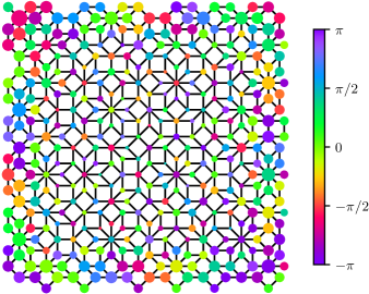
Figure 1: An edge state of a magnetic Hamiltonian on a finite patch of the Ammann-Beenker tiling ($L=9$). The color of the dots corresponds to the phase of the wave function and the radius to the modulus. While the infinite system has a spectral gap at this energy, the finite system has an eigenstate whose mass is concentrated at the edges.

Numerical investigations of aperiodic systems necessarily restrict the Hamiltonian to finite patches and then either apply periodic boundary conditions, or use open boundary conditions. The first method relies on the construction of the so-called periodic approximant systems. While it has been shown that in specific models it is possible to successfully construct such periodic approximants [13, 14], the mathematical justification of this procedure for generic aperiodic systems is still subject of ongoing works [15, 16, 17, 18]. Furthermore, we stress that usually one does not have a precise control of the rate of convergence of the spectral properties of the periodic approximants. Using open boundary conditions, on the other hand, edge-states may appear in gaps of the bulk spectrum, i.e. in the spectrum of the infinite volume Hamiltonian. In previous works, such edge-states, as shown for example in Figure 1, have been discarded as “spectral pollution” [8, 19]. So far, however, no precise criterion has been formulated to decide whether a given state is an edge state and thus does not contribute to the bulk spectrum. Our result formulated below yields such a criterion. Roughly speaking we show that if for some spectral window all quasi-modes appearing in boxes of side-length $2L$ satisfy a quantifiable “edge-state criterion”, then this spectral window is a gap in the spectrum of the infinite volume Hamiltonian. Our criterion can be numerically checked for finite-range Hamiltonians with finite local complexity, where for a given $L>0$ the restriction of $H$ to a box of side-length $2L$ centred at an arbitrary point in space yields a matrix from a finite set of possible realizations.

We first formulate a general finite-size criterion which is equivalent to the existence of a bulk gap. For this we merely assume that the Hamiltonian $H$ is a bounded hermitian operator on $\ell^{2}(\Gamma;\mathcal{H})$, where $\mathcal{H}$ is a separable Hilbert space and $\Gamma\subset\mathbb{R}^{d}$ is a countable set. We will also assume that there is a maximal distance $r>0$ such that any point in $\mathbb{R}^{d}$ is within a distance at most $r$ of a point in $\Gamma$. Throughout this article we measure distances in $\mathbb{R}^{d}$ using the $\infty$-norm $\|x\|_{\infty}:=\max\{|x_{1}|,\ldots,|x_{d}|\}$. We also write $B_{L}(x):=\prod_{j=1}^{d}(x_{j}-L,x_{j}+L)$ for the open cube of side length $2L$ centered around the point $x\in\mathbb{R}^{d}$ and $\overline{B_{L}}(x)$ for its closure. For any set $A\subset\mathbb{R}^{d}$ and wave function $\psi\in\ell^{2}(\Gamma;\mathcal{H})$, we denote by $\left\lVert\psi\right\rVert_{A}^{2}:=\sum_{x\in\Gamma\cap A}\|\psi(x)\|_{\mathcal{H}}^{2}$ its $\ell^{2}$-mass in $A$.

Definition 1.

Let $\epsilon,L>0$ and $\lambda\in\mathbb{R}$. We say that a Hamiltonian $H$ is $\epsilon$-bulk-gapped at energy $\lambda$ and scale $L$, if there exist constants $N\in\mathbb{N}$, $N\geq 2$, and ${C<{1/N^{d}}}$, such that for any $x\in\Gamma$ and any ${\psi\in\ell^{2}(\Gamma;\mathcal{H})}$ we have the following implication: Whenever

$$\left\lVert(H-\lambda)\psi\right\rVert_{B_{L}(x)}\leq\epsilon\left\lVert\psi\right\rVert_{B_{L}(x)}\,,$$ (1)

then for $l:=\frac{L+r}{N}+r$ it holds that

$$\left\lVert\psi\right\rVert_{\overline{B_{l}}(x)}^{2}\leq C\left\lVert\psi\right\rVert_{B_{L}(x)}^{2}\,.$$ (2)

In words, Definition 1 requires that at some scale $L$ all $\epsilon$-quasi-modes (1) have an underproportional mass within the bulk (2). Although this property depends only on evaluations of the Hamiltonian $H$ on finite patches, we can show that it implies that the interval $(\lambda-\epsilon,\lambda+\epsilon)$ does not contain any spectrum of $H$.

Theorem 1.

If a Hamiltonian $H$ on $\ell^{2}(\Gamma;\mathcal{H})$ is locally $\epsilon$-bulk-gapped at energy $\lambda$ on some scale $L>0$, then the interval $(\lambda-\epsilon,\lambda+\epsilon)$ is a gap in the spectrum of $H$, i.e.

$$\sigma(H)\cap(\lambda-\epsilon,\lambda+\epsilon)=\varnothing.$$

The proof of Theorem 1 is given in the supplemental material, Section 1. To explain its simple geometric idea, suppose that we are in dimension $d=1$, and that the statement in Definition 1 holds for $l=L/N$ instead of the more complicated expression involving $r$. We can then show that $H$ has no eigenvalues in $(\lambda-\epsilon,\lambda+\epsilon)$ using a simple decomposition argument: Define the lattices

$$Z_{q}=2L(\mathbb{Z}+q/N)\quad\text{for}\quad q\in\{1,\dots,N\}\,.$$

While for fixed $q$ the larger open intervals $B_{L}(x)$ centred at different $x\in Z_{q}$ are still mutually disjoint, the shorter closed intervals $\overline{B_{l}}(x)$ cover $\mathbb{R}$ when taking the union over all $q$, i.e.

$$\bigcup\nolimits_{q=1}^{n}\bigcup\nolimits_{x\in Z_{q}}\overline{B_{l}}(x)=\mathbb{R}\,.$$ (3)

Now assume that $\psi$ is an eigenfunction of $H$ with eigenvalue $\lambda_{0}\in(\lambda-\epsilon,\lambda+\epsilon)$. Then $\psi$ satisfies (1) for any $x$, and thus, by assumption, also (2). This implies

$$\sum_{q=1}^{N}\sum_{x\in Z_{q}}\left\lVert\psi\right\rVert^{2}_{\overline{B_{l}}(x)}<\frac{1}{N}\sum_{q=1}^{N}\sum_{x\in Z_{q}}\left\lVert\psi\right\rVert^{2}_{B_{L}(x)}=\left\lVert\psi\right\rVert^{2}\,,$$

while (3) implies

$$\sum_{q=1}^{N}\sum_{x\in Z_{q}}\left\lVert\psi\right\rVert^{2}_{\overline{B_{l}}(x)}\geq\left\lVert\psi\right\rVert^{2}\,.$$

This is a contradiction and thus no such eigenfunction can exist.

We now discuss how to establish existence of local $\epsilon$-bulk-gaps, and thus by Theorem 1 spectral gaps for Hamiltonians with finite range hoppings and finite local complexity. We first give a sufficient condition for a Hamiltonian to be locally $\epsilon$-bulk-gapped that can be efficiently verified numerically. From now on we assume that $H$ has only finite range hoppings with maximal hopping length $m$, namely $H_{xy}=0$ for all $x,y\in\Gamma$ with $\|x-y\|_{\infty}>m$. For any set $A\subset\mathbb{R}^{d}$ we denote by $\mathbf{1}_{A}$ the characteristic function of $A$ and set $H_{A}:=\mathbf{1}_{A}H\mathbf{1}_{A}$.

Proposition 1.

As before, let $L>0$, $N\in\mathbb{N}$, $N\geq 2$, ${l:=\frac{L+r}{N}+r}$, and $\lambda\in\mathbb{R}$.
Assume that for every $x\in\Gamma$ there exists a set $A(x)\subset\Gamma$ such that $\overline{B_{l}}(x)\subseteq A(x)\subseteq B_{L-m}(x)$, $\lambda\notin\sigma(H_{A(x)})$, and

$$D(x)=\left\lVert\mathbf{1}_{\overline{B_{l}}(x)}(H_{A(x)}-\lambda)^{-1}\mathbf{1}_{A(x)}H\mathbf{1}_{B_{L}(x)\backslash A(x)}\right\rVert_{\mathrm{op}}$$

satisfies $D(x)<N^{-d/2}$.
Then $H$ is $\epsilon$-bulk-gapped at energy $\lambda$ and scale $L$ for any $\epsilon>0$ with

$$\epsilon<\inf_{x\in\Gamma}\frac{N^{-d/2}-D(x)}{\left\lVert\mathbf{1}_{\overline{B_{l}}(x)}(H_{A(x)}-\lambda)^{-1}\mathbf{1}_{A(x)}\right\rVert_{\mathrm{op}}}\,.$$ (4)

The proof of Proposition 1 is given in the supplemental material, Section 1. Note that $H_{A(x)}$ is a sparse matrix and therefore the conditions of Proposition 1 can be efficiently checked using a sparse LU factorization [20], allowing computations for values of $L$ for which a direct diagonalization approach would no longer be computationally feasible.

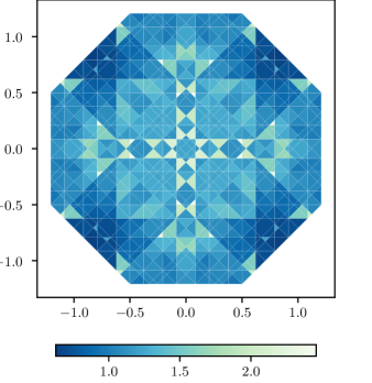
Figure 2: The octagonal acceptance region for the Ammann-Beenker tiling decomposed into subpolygons corresponding to the different local patches in $\mathcal{C}_{L}(x)$, for $L=5$. The color of each polygon corresponds to $D(x)$ computed for ${N=2}$ with $A(x)=B_{L-1}(x)$ (in this case $m=1$), drawn in a logarithmic scale with base $10$, for the Hofstadter Hamiltonian at magnetic field $b=1$ and energy $1.5$. At scale $L=5$, $D(x)$ never falls below the required bound $1/2$. At scale $L=50$ one finds that $D(x)<1/2$ for every local patch, proving the gap.

In order to apply Proposition 1 to quasicrystals $\Gamma\subset\mathbb{R}^{d}$, we still need to find a way to determine all local patches at scale $L$,

$$\mathcal{C}_{L}(x)=\{y\in\mathbb{R}^{d}\,|\,x+y\in\Gamma\cap B_{L}(x)\}\subset B_{L}(0)\,,$$

that occur for $x\in\Gamma$. We say that $\Gamma$ has finite local complexity if the set $\mathcal{C}_{L}=\{\mathcal{C}_{L}(x)\,|\,x\in\Gamma\}$ is finite [21, 22, 23]. Those quasiperiodic tilings that are suggested as models for physical systems all have finite local complexity. Our method is practical because, for common quasicrystals, the number of local patches grows only polynomially in $L$, while it would grow exponentially without long-range order [24, 25].

To enumerate the tilings, we make use of the cut-and-project construction of quasiperiodic tilings [26, 27]. The Ammann-Beenker tiling [28, 29] can be defined by a cut-and-project method using two “projections”,

$$p=\begin{pmatrix}1&a&0&-a\\ 0&a&1&a\end{pmatrix}\quad\mbox{and}\quad\kappa=\begin{pmatrix}1&-a&0&a\\ 0&a&-1&a\end{pmatrix},$$

both maps from $\mathbb{R}^{4}$ to $\mathbb{R}^{2}$, where $a=1/\sqrt{2}$. We call $p$ and $\kappa$ “projections” since they represent orthogonal projections onto two orthogonal two-dimensional subspaces of $\mathbb{R}^{4}$ which are then both identified with $\mathbb{R}^{2}$. Furthermore, let $R\subset\mathbb{R}^{2}$ be the regular axis-aligned octagon centered at $0$ with side length $1$. The vertices of the Ammann-Beenker tiling are the set

$$\Gamma_{\mathrm{AB}}=\big{\{}\,p(z)\;\big{|}\;z\in\mathbb{Z}^{4},\,\kappa(z)\in R\,\big{\}}\,.$$

An edge is introduced between $p(z_{1})$ and $p(z_{2})$ whenever $z_{1}$ and $z_{2}$ differ by a unit vector in $\mathbb{R}^{4}$. Because $a$ is irrational, every point $x\in\Gamma_{\mathrm{AB}}$ has exactly one pre-image $z\in\mathbb{Z}^{4}$ such that $p(z)=x$.

What local patches $\mathcal{C}_{L}(x)$ can occur when $x$ varies in $\Gamma_{\mathrm{AB}}$? Let $z\in\mathbb{Z}^{4}$ be such that $p(z)=x\in\Gamma_{\mathrm{AB}}$, and consider the set of all $v\in\mathbb{Z}^{4}$ such that $p(z+v)\in\Gamma_{\mathrm{AB}}\cap B_{L}(x)$. There is only a finite number of $v\in\mathbb{Z}^{4}$ that can occur across all $x$, because $v$ has to fulfil the two conditions

$$p(z+v)\in B_{L}(x)\quad\text{and}\quad\kappa(z+v)\in R.$$ (5)

By the linearity of $p$, the first condition reduces to

$$p(v)\in B_{L}(0)$$ (6)

and since $\kappa(x)\in R$, the second condition implies

$$\kappa(v)\in 2R\,,$$ (7)

where $2R$ is the octagon of side length 2.

Both (6) and (7) state that a linear image of $v$ lies in some compact set. Since $p$ and $\kappa$ have orthogonal kernels, these two conditions define a set $\tilde{V}_{L}$ linearly equivalent to the cartesian product of $B_{L}(0)$ and $2R$, which is itself compact and hence contains only finitely many integer points. Let $V_{L}=\tilde{V}_{L}\cap\mathbb{Z}^{4}$ be this set of “candidate points”. An algorithm for computing $V_{L}$ is described in the supplemental material, Section 2, Algorithm 1.

According to (5), for any $v\in V_{L}$ the patch $\mathcal{C}_{L}(x)$ contains the point $p(z+v)$ if and only if

$$\kappa(z)\in R-\kappa(v)\,,$$ (8)

i.e. if $\kappa(z)$ lies in the shifted octagon $R-\kappa(v)$. Put differently, every candidate point $v\in V_{L}$ decomposes the octagon $R$ into two disjoint sets $P^{0}(v)$ and $P^{1}(v)$, delineating for which $\kappa(z)$ the point $p(z+v)$ is or is not in $\Gamma_{\mathrm{AB}}$. The enumeration algorithm then merely consists of computing all possible intersections $\bigcap_{v\in V}P^{i_{v}}(v)$, where $i\in\{0,1\}^{|V|}$. One can show that the number of such intersection that are nonempty, and hence the number of local patches, grows quadratically in $L$ for the Ammann-Beenker tiling [30]. They can be enumerated efficiently using a dynamic programming approach described in Section 2, Algorithm 2 of the supplemental material. Figure 2 shows the resulting decomposition of the octagon $R$ for $L=5$.

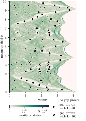
Figure 3: The Hofstadter butterfly of the magnetic Laplacian on the Ammann-Beenker tiling with some points selected for investigation using our method.

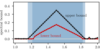
Figure 4: Comparison of our lower bound for the distance to spectrum (for $L=50$) to the upper bound computed with the method of [8]. We computed both bounds for 50 equally spaced energies in the Hofstadter model at a constant magnetic field $b=1$. The combination of these bounds allows us to bound the extent of the spectral gap containing energy $1.5$. The endpoints of the gap must be contained in the lighter shaded areas around energies $1.2$ and $1.82$. A similar plot for the Fibonacci crystal is shown in Figure S1 in the supplemental material.

We now study two physical systems on the Ammann-Beenker tiling. The $p_{x}p_{y}$-model is a model for a weak topological superconductor whose real-space description allows it to be defined on aperiodic sets [31]. The matrix elements of the Hamiltonian are

$$H_{xy}=-t\sigma_{3}-\tfrac{\mathrm{i}}{2}\Delta\sigma_{1}\cos(\alpha_{xy})-\tfrac{\mathrm{i}}{2}\Delta\sigma_{2}\sin(\alpha_{xy})\,,$$

$$H_{xx}=-\mu\sigma_{3}\,,$$

for $\|x-y\|_{2}\leq 1$, and $H_{xy}=0$ otherwise. Here $\sigma_{1},\sigma_{2},\sigma_{3}$ are Pauli matrices, $\mu,\Delta\in\mathbb{R}$ and $\alpha_{xy}$ is the signed angle between the edge $xy$ and the $e_{1}$-axis.

For $\mu$ very large, this Hamiltonian can be considered as a small perturbation of $\mu\sigma_{3}$, thus its spectrum has a gap around 0, without edge states when restricted to finite domains. As $\mu$ decreases, the gap eventually closes and the system is expected to undergo a quantum phase transition into a topologically nontrivial phase. This topological regime has been studied in [7]. Employing computational $K$-theory, convincing evidence was found that a large gap around zero indeed reopens. But the numerical data also suggested a second small gap might open. In the absence of a decisive criterion, the author had to leave open whether this gap persists in the thermodynamic limit [7, p. 9]. Using our method, we could prove that there really is a small second gap around energy $0.804$ in the infinite system.

As a second example, we applied our method to the Hofstadter model on the Ammann-Beenker tiling. In the symmetric gauge, the matrix elements of the Hofstadter Hamiltonian are $H_{xy}=\mathrm{e}^{\mathrm{i}b\det(x,y)}$ for $\|x-y\|_{2}\leq 1$, and $H_{xy}=0$ otherwise, where $b\in\mathbb{R}$ denotes the strength of the magnetic field perpendicular to the tiling. It was previously observed that patterns related to the Hofstadter butterfly also emerge in quasicrystalline systems [32, 33]. We approximated the density of states of the Hofstadter butterfly (see Figure 3) by diagonalization of a finite system and created a set of possible gap locations by taking all local minima of a kernel density estimate with bandwidth $0.1$ of the spectra. In this way we generated 187 combinations of magnetic field and energy where a gap might be expected. Applying our algorithm with $L=50$, we could show for 44 of these points that there is a spectral gap in the infinite system, increasing to 49 points with $L=100$. For $L=50$, this required checking 15,139 local patches, while for $L=100$, we had $|\mathcal{C}_{L}|=60{,}601$.

We also computed a cross-section of our bound at different energies for a fixed magnetic field (see Figure 4). Comparing our lower bound on the distance to spectrum to the upper bound in [8] showed that the curves are similar and increase linearly towards the center of the gap. The combination of both bounds yields rigorous and precise information on the positions of the edge of the spectral gap. As discussed in the Section 4 of the supplemental material, one can indeed deduce from our result that the problem of determining the spectrum of an operator with finite local complexity has a solvability complexity index [34] equal to one. In particular, this means that for any energy $\lambda$ that is not in the spectrum, one can determine an $L$ such that our algorithm applied on the scale $L$ proves that some neighborhood of $\lambda$ is contained in a gap. Together with the convergence result of [8], this means that the gap estimate in Figure 4 can be made arbitrarily accurate by choosing $L$ large enough.

In conclusion, we have described a new way to prove the existence of spectral gaps in infinitely extended quasicrystalline systems based on numerical computations on finite patches. The algorithm exploits the fact that in systems of finite local complexity, the spectral gaps of the bulk operator can be derived from the structure of the eigenstates of its restrictions to patches of a fixed finite size. In this way, we circumvent the no-go theorem of [8], which states that there is no algorithm that computes spectral gaps in general infinitely extended systems.

References

- Sire [1989] C. Sire, Electronic spectrum of a 2d quasi-crystal related to the octagonal quasi-periodic tiling, EPL 10, 483 (1989).
- Sire and Bellissard [1990] C. Sire and J. Bellissard, Renormalization group for the octagonal quasi-periodic tiling, EPL 11, 439 (1990).
- Benza and Sire [1991] V. G. Benza and C. Sire, Band spectrum of the octagonal quasicrystal: Finite measure, gaps, and chaos, Phys. Rev. B 44, 10343 (1991).
- Zoorob et al. [2000] M. E. Zoorob, M. D. B. Charlton, G. J. Parker, J. J. Baumberg, and M. C. Netti, Complete photonic bandgaps in 12-fold symmetric quasicrystals, Nature 404, 740 (2000).
- Man et al. [2005] W. Man, M. Megens, P. J. Steinhardt, and P. M. Chaikin, Experimental measurement of the photonic properties of icosahedral quasicrystals, Nature 436, 993 (2005).
- Fuchs and Vidal [2016] J.-N. Fuchs and J. Vidal, Hofstadter butterfly of a quasicrystal, Phys. Rev. B 94, 205437 (2016).
- Loring [2019] T. A. Loring, Bulk spectrum and K-theory for infinite-area topological quasicrystals, J. Math. Phys. 60, 081903 (2019).
- Colbrook et al. [2019] M. J. Colbrook, B. Roman, and A. C. Hansen, How to Compute Spectra with Error Control, Phys. Rev. Lett. 122, 250201 (2019).
- Trefethen and Embree [2020] L. N. Trefethen and M. Embree, Spectra and pseudospectra (Princeton University Press, 2020).
- Bandres et al. [2016] M. A. Bandres, M. C. Rechtsman, and M. Segev, Topological photonic quasicrystals: fractal topological spectrum and protected transport, Phys. Rev. X 6 (2016).
- Kellendonk and Prodan [2019] J. Kellendonk and E. Prodan, Bulk–boundary correspondence for sturmian kohmoto-like models, Ann. Henri Poincaré 20, 2039 (2019).
- Zilberberg [2021] O. Zilberberg, Topology in quasicrystals, Opt. Mater. Express 11, 1143 (2021).
- Duneau [1989] M. Duneau, Approximants of quasiperiodic structures generated by the inflation mapping, J. Phys. A 22, 4549 (1989).
- Tsunetsugu et al. [1991] H. Tsunetsugu, T. Fujiwara, K. Ueda, and T. Tokihiro, Electronic properties of the penrose lattice. i. energy spectrum and wave functions, Phys. Rev. B 43, 8879 (1991).
- Prodan [2012] E. Prodan, Quantum transport in disordered systems under magnetic fields: a study based on operator algebras, Appl. Math. Res. Express (2012).
- Beckus et al. [2018] S. Beckus, J. Bellissard, and G. De Nittis, Spectral Continuity for Aperiodic Quantum Systems I. General Theory, J. Funct. Anal. 275, 2917 (2018).
- Beckus et al. [2019] S. Beckus, J. Bellissard, and H. Cornean, Hölder Continuity of the Spectra for Aperiodic Hamiltonians, Ann. Henri Poincaré 20, 3603 (2019).
- Loring and Schulz-Baldes [2020] T. A. Loring and H. Schulz-Baldes, The spectral localizer for even index pairings, J. Noncommutative Geom. 14, 1 (2020).
- Davies [2004] E. B. Davies, Spectral pollution, IMA J. Numer. Anal. 24, 417 (2004).
- Li [2005] X. S. Li, An Overview of SuperLU: Algorithms, Implementation, and User Interface, ACM T. Math. Software 31, 302 (2005).
- Lagarias [1999] J. C. Lagarias, Geometric models for Quasicrystals I. Delone sets of finite type, Discrete Comput. Geom. 21, 161 (1999).
- Baake and Moody [1998] M. Baake and R. V. Moody, Diffractive point sets with entropy, J. Phys. A - Math. Gen. 31, 9023 (1998).
- Lagarias and Pleasants [2002] J. C. Lagarias and P. A. B. Pleasants, Local Complexity of Delone Sets and Crystallinity, Can. Math. Bull. 45, 634–652 (2002).
- Elser [1985] V. Elser, Comment on “Quasicrystals: A new class of ordered structures”, Phys. Rev. Lett. 54, 1730 (1985).
- Moody [2000] R. V. Moody, Model Sets: A Survey, in From quasicrystals to more complex systems (Springer, 2000) pp. 145–166.
- de Bruijn [1981] N. G. de Bruijn, Algebraic theory of Penrose’s non-periodic tilings of the plane, Indag. Math. 84, 39 (1981).
- Janot [2012] C. Janot, Quasicrystals: A Primer, 2nd ed. (Oxford University Press, 2012).
- Ammann et al. [1992] R. Ammann, B. Grünbaum, and G. C. Shephard, Aperiodic tiles, Discrete Comput. Geom. 8, 1 (1992).
- Beenker [1982] F. P. M. Beenker, Algebraic theory of non-periodic tilings of the plane by two simple building blocks: a square and a rhombus, Technical Report 82-WSK-04 (Eindhoven University of Technology, 1982).
- Julien [2010] A. Julien, Complexity and Cohomology for Cut-and-Projection Tilings, Ergodic Theory and Dynamical Systems 30, 489 (2010).
- Fulga et al. [2016] I. C. Fulga, D. I. Pikulin, and T. A. Loring, Aperiodic weak topological superconductors, Phys. Rev. Lett. 116, 257002 (2016).
- Vidal and Mosseri [2004] J. Vidal and R. Mosseri, Quasiperiodic tilings in a magnetic field, J. Non-Cryst. Solids 334–335, 130 (2004).
- Tran et al. [2015] D.-T. Tran, A. Dauphin, N. Goldman, and P. Gaspard, Topological Hofstadter insulators in a two-dimensional quasicrystal, Phys. Rev. B 91, 085125 (2015).
- Hansen [2011] A. Hansen, On the solvability complexity index, the n-pseudospectrum and approximations of spectra of operators, J. Am. Math. Soc. 24, 81 (2011).