GNN-Enhanced Approximate Message Passing for Massive/Ultra-Massive MIMO Detection

Abstract

Efficient massive/ultra-massive multiple-input multiple-output (MIMO) detection algorithms with satisfactory performance and low complexity are critical to meet the high throughput and ultra-low latency requirements in 5G and beyond communications, given the extremely large number of antennas. In this paper, we propose a low complexity graph neural network (GNN) enhanced approximate message passing (AMP) algorithm, AMP-GNN, for massive/ultra-massive MIMO detection. The structure of the neural network is customized by unfolding the AMP algorithm and introducing the GNN module for multiuser interference cancellation. Numerical results will show that the proposed AMP-GNN significantly improves the performance of the AMP detector and achieves comparable performance as the state-of-the-art deep learning-based MIMO detectors but with reduced computational complexity. Furthermore, it presents strong robustness to the change of the number of users.

I Introduction

Massive/Ultra-massive multiple-input multiple-output (MIMO) communication has become one of the enabling technologies for 5G and beyond networks owing to the high spectral efficiency and link reliability. Given the increasing size of antenna arrays, efficient MIMO detection algorithms are of significant importance to unleash the full potential of MIMO systems, and a series of research has been conducted to balance the performance and complexity [1, 2, 3]. To this end, iterative detectors based on approximate message passing (AMP) [4] and expectation propagation (EP) [5] have been proposed. The AMP-based detector [2] is of low complexity and easy to implement in practice because only the matrix-vector multiplication is involved. However, it only favors the scenario when the elements of the MIMO channel matrix follow independent identically distributed (i.i.d.) sub-Gaussian distribution with zero mean. In contrast, the EP-based detector [3] achieves Bayes-optimal performance when the channel matrix is unitarily invariant, but has a higher complexity than the AMP-based detector owing to involves a matrix inversion.

Owing to its strong ability to extract useful features from data, deep learning (DL) has been recently utilized in the physical layer design of wireless communications [6, 7, 8], such as millimeter-wave channel estimation [9], channel state information (CSI) feedback [10], and data detection [11]. For MIMO detection, it has been shown that DL can improve traditional message passing detectors, such as AMP, and EP, with different strategies. Specifically, the OAMP-Net and OAMP-Net2 detectors [11] were developed by unfolding the OAMP detector and introducing several learnable parameters. However, the performance improvements are still limited owing to small number of learnable variables.

Recently, graph neural networks (GNNs) have been applied to wireless communications [12], such as to learn a message-passing solution for inference problems [13, 14]. In particular, a GNN-based MIMO detector was developed by utilizing a pair-wise Markov random field (MRF) model [13]. As GNNs can capture the structure of the data into the feature vectors for the nodes and update them through message-passing methods, they are very promising solutions for enhancing the performance of the message-passing-based detectors. For example, the GEPNet was developed by incorporating the GNN into the EP detector[14]. However, the computational complexity of GEPNet is still high because of the matrix inversion in each layer. An efficient DL-based MIMO detection algorithm, which strikes a good balance between the performance and complexity, is by far not available.

In this paper, we develop a model-driven DL-based MIMO detector, AMP-GNN, where the neural network structure is obtained by unfolding the AMP detector and incorporating the GNN module. In particular, the GNN module receives the equivalent AWGN observation from the AMP as input and outputs a refined version back to AMP at each layer. It can improve the accuracy of the equivalent AWGN observation for AMP algorithm. As a result, it is helpful for multi-user interference (MUI) cancellation. The AMP-GNN also inherits the low-complexity of the AMP detector and improves the performance with the GNN module. Simulation results shall demonstrate that the proposed AMP-GNN significantly outperforms existing the AMP detector and achieve comparable performance as the state-of-the-art GEPNet detector while reducing the computational complexity.

Notations—For any matrix $\mathbf{A}$, $\mathbf{A}^{T}$, $\mathbf{A}^{*}$, and ${\mathrm{tr}}(\mathbf{A})$ will denote the transpose, conjugate, and trace of $\mathbf{A}$, respectively. In addition, $\mathbf{I}$ is the identity matrix, $\mathbf{0}$ is the zero matrix, and $\mathbf{1}_{n}$ is the $n$-dimensional all-ones vector. A proper complex Gaussian distribution with mean $\boldsymbol{\mu}$ and covariance $\boldsymbol{\Omega}$ can be described by the probability density function (pdf):

$$\mathcal{N}_{\mathbb{C}}(\mathbf{z};\boldsymbol{\mu},\boldsymbol{\Omega})=\frac{1}{\mathrm{det}(\pi\boldsymbol{\Omega})}e^{-(\mathbf{z}-\boldsymbol{\mu})^{H}\boldsymbol{\Omega}^{-1}(\mathbf{z}-\boldsymbol{\mu})}$$

II Problem Formulation and Algorithm Review

In this section, we first formulate the MIMO detection problem by adopting a Bayesian inference. To better understand the proposed AMP-GNN, we will review the AMP-based MIMO detector.

II-A MIMO Detection

We assume an uplink multi-user MIMO (MU-MIMO) systems where the base station (BS) equips $M$ antennas sevres $N$ single-antenna users. The symbol vector ${\mathbf{x}}\in\mathbb{C}^{N\times 1}$ is transmitted over a Rayleigh fading channel ${\mathbf{H}}\in\mathbb{C}^{M\times N}$. Each element of ${\mathbf{H}}$ and ${\mathbf{x}}$ are drawn from an i.i.d. complex Gaussian distribution and the $Q$-QAM constellation, respectively. The received signal ${\mathbf{y}}\in\mathbb{C}^{M\times 1}$ is given by

$${\mathbf{y}}={\mathbf{H}}{\mathbf{x}}+{\mathbf{n}},$$ (1)

where ${\mathbf{n}}\sim\mathcal{N}_{\mathbb{C}}(0,\sigma^{2}\mathbf{I}_{M})$ is the additive white Gaussian noise (AWGN). Based on the Bayes’ theorem, the posterior probability $p(\mathbf{x}|\mathbf{y},\mathbf{H})$ can be factorized as

$$p(\mathbf{x}|\mathbf{y},\mathbf{H})=\frac{p(\mathbf{y}|\mathbf{x},\mathbf{H})p(\mathbf{x})}{p(\mathbf{y}|{\mathbf{H}})}=\frac{p(\mathbf{y}|\mathbf{x},\mathbf{H})p(\mathbf{x})}{\int p(\mathbf{y}|\mathbf{x},\mathbf{H})p(\mathbf{x})d\mathbf{x}}.$$ (2)

Given the posterior probability $p(\mathbf{x}|\mathbf{y},\mathbf{H})$, the Bayesian MMSE estimate is obtained by

$$\hat{\mathbf{x}}=\int\mathbf{x}p(\mathbf{x}|\mathbf{y},\mathbf{H})d\mathbf{x}.$$ (3)

However, the Bayesian MMSE estimator is computationally intractable because the MMSE estimation in (3) involves a high-dimensional integral. In [4], the AMP algorithm was proposed as an efficient alternative to recover signal $\mathbf{x}$. We will introduce the AMP-based detector in the following subsection.

II-B AMP-Based MIMO Detector

1. Input: ${\mathbf{y}}$, ${\mathbf{H}}$, $\sigma^{2}$, $\mathcal{P}({\mathbf{x}})$.

2. Initialization: $\hat{x}_{n}^{(1)}=0$, $\hat{v}_{n}^{(1)}=\frac{N}{M}$, $Z_{m}^{(0)}=y_{m}$.

3. Output: $\hat{{\mathbf{x}}}^{(T)}$.

4. Iteration:

for $t=1,\cdots,T$ do

      

$$V_{m}^{(t)} =\sum_{n=1}^{N}|h_{mn}|^{2}\hat{v}_{n}^{(t)}$$ (4a)

$$Z_{m}^{(t)} =\sum_{n=1}^{N}h_{mn}\hat{x}_{n}^{(t)}-\frac{V_{m}^{(t)}(y_{m}-Z_{m}^{(t-1)})}{\sigma^{2}+V_{m}^{(t-1)}}$$ (4b)

$$\Sigma_{n}^{(t)} =\left(\sum_{m=1}^{M}\frac{|h_{mn}|^{2}}{\sigma^{2}+V_{m}^{(t)}}\right)^{-1}$$ (4c)

$$r_{n}^{(t)} =\hat{x}_{n}^{(t)}+\Sigma_{n}^{(t)}\sum_{m=1}^{M}\frac{h_{mn}^{*}(y_{m}-Z_{m}^{(t)})}{\sigma^{2}+V_{m}^{(t)}}$$ (4d)

$$\hat{x}_{n}^{(t+1)} =\mathbb{E}\{x_{n}|r_{n}^{(t)},\Sigma_{n}^{(t)}\}$$ (4e)

$$\hat{v}_{n}^{(t+1)} =\text{Var}\{x_{n}|r_{n}^{(t)},\Sigma_{n}^{(t)}\}$$ (4f)

Algorithm 1 AMP-based MIMO detector

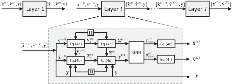
Figure 1: .  The structure of the proposed AMP-GNN detector.

The AMP algorithm has been proposed to solve sparse linear inverse problems in compressed sensing [4]. In Algorithm  1, we summarize the AMP algorithm for MIMO detection, where $m$ and $n$ are the indexes of the antenna in the BS and users, respectively. The main principle of the algorithm is to decouple the posterior probability $p(\mathbf{x}|\mathbf{y},\mathbf{H})$ into a series of $p(x_{n}|\mathbf{y},\mathbf{H}),(n=1,2,\ldots,N)$, in an iterative way. In particular, $p(x_{n}|\mathbf{y},\mathbf{H})$ is assumed to be a Gaussian distribution and obtained from the equivalent AWGN model

$$r_{n}^{(t)}=x_{n}+w_{n}^{(t)},$$ (5)

where $w_{n}^{(t)}\sim\mathcal{N}_{\mathbb{C}}(w_{n}^{(t)};0,\Sigma_{n}^{(t)})$.

To better understand Algorithm 1, we first provide a brief explanation for each equation in Algorithm 1 with the detailed derivation given in [4]. Specifically, (4a) and (4b) compute the variance and mean estimation for ${\mathbf{z}}={\mathbf{H}}{\mathbf{x}}$, respectively. Then, (4c) calculates the equivalent noise variance $\Sigma_{n}^{(t)}$ while (4d) gives the equivalent AWGN observation $r_{n}^{(t)}$. Finally, (4e) and (4f) perform the posterior mean and variance estimation for the equivalent AWGN model (5). As the transmitted symbol is assumed to be drawn from the $Q$-QAM set $\mathcal{S}=\{s_{1},s_{2},\ldots,s_{Q}\}$, the results in (4e) and (4f) are given by

$$\hat{x}^{(t+1)}_{n}=\frac{\sum_{s_{i}\in\mathcal{S}}s_{i}\mathcal{N}_{{\mathbb{C}}}(s_{i};r_{n}^{(t)},\Sigma_{n}^{(t)})p(s_{i})}{\sum_{s_{i}\in\mathcal{S}}\mathcal{N}_{{\mathbb{C}}}(s_{i};r_{n}^{(t)},\Sigma_{n}^{(t)})p(s_{i})},$$ (6)

$$\hat{v}^{(t+1)}_{n}=\frac{\sum_{s_{i}\in\mathcal{S}}|s_{i}|^{2}\mathcal{N}_{{\mathbb{C}}}(s_{i};r_{n}^{(t)},\Sigma_{n}^{(t)})p(s_{i})}{\sum_{s_{i}\in\mathcal{S}}\mathcal{N}_{{\mathbb{C}}}(s_{i};r_{n}^{(t)},\Sigma_{n}^{(t)})p(s_{i})}-|\hat{x}^{(t+1)}_{n}|^{2}.$$ (7)

As can be observed in Algorithm  1, the performance of the AMP-based MIMO detector is mainly determined by the accuracy of the assumed equivalent AWGN model (5). In [4], it was shown that the equivalent AWGN model is asymptotically accurate when the dimensions of the system tend to infinity, i.e., $M,N\rightarrow\infty$. However, in practical MIMO systems especially with high MUI, the performance of the AMP-based MIMO detector is far from optimal and even has an error floor owing to the inaccurate assumption. These observations motivate us to improve the AMP-based MIMO detector with the DL technique, especially GNNs.

III AMP-GNN Detector

In this section, we propose an AMP-GNN detector for MIMO detection. First, we present the network structure of the AMP-GNN detector and introduce the GNN module in detail. Then, the computational complexity of the AMP-GNN is analyzed and compared with other MIMO detectors.

III-A AMP-GNN Architecture

Given the important advantages of GNNs, such as learning to capture the MUI information, here we exploit them to improve the AMP detector in this article. The block diagram of the AMP-GNN is illustrated in Fig. 1. Specifically, the network consists of $T$ cascade layers, and each layer has the same structure that contains a GNN module and a conventional AMP algorithm shown in Algorithm  1. In particular, the input of the AMP-GNN is the received signal $\mathbf{y}$ and the initial value is set as $\hat{\mathbf{x}}^{(1)}=\mathbf{0}$ and $\hat{\mathbf{v}}^{(1)}=\frac{N}{M}\mathbf{1}_{N}$, and the output is the final estimate $\hat{\mathbf{x}}^{(T)}$ of signal $\mathbf{x}$. For the $t$-th layer of the AMP-GNN, the inputs are the estimated signal $\hat{\mathbf{x}}^{(t-1)}$ and $\hat{\mathbf{v}}^{(t-1)}$ from the $(t-1)$-th layer and the received signal $\mathbf{y}$. As we have introduced the AMP-based MIMO in Section II-B, we will introduce the GNN module in the next subsection.

III-B The GNN Module

GNNs have been recently adopted in wireless communications as they can incorporate the graph topology of the wireless network into the neural network design [12]. The GNN model adopted in the AMP-GNN is called the message passing neural network (MPNN) and the message passing rules are illustrated in Fig. 2. Similar to [13], the GNN in the AMP-GNN is composed of three main modules: a propagation module, an aggregation module, and a readout module. The first two modules operate at all layers while the readout module is involved only after the last layer. To better understand the structure of the MPNN, we first elaborate the following concepts about the GNN.

• Node: Each node $n\in V$ represents the $n$-th user.

• Node attributes: Each node has an assigned node attribute ${\mathbf{a}}_{n}$ that is constant when exchange the information between nodes. In proposed AMP-GNN, the GNN in $t$-layer takes the output from the linear module in AMP algorithm as node attribute.

• Edge: An edge $e_{n,j}\in E$ is to connect node $n\in V$ and $j\in V$.

• Edge attributes: Each edge $e_{n,j}$ has an assigned edge attribute $\mathbf{f}_{jn}$ that is constant when compute the message. In proposed AMP-GNN, the GNN use the CSI and noise level as edge attribute.

• Hidden vector: Each node ${\mathbf{U}}_{n}$ has a hidden vector updated in the different round of the GNN, and will be used to compute the output of the GNN.

• Message: The incoming messages ${\mathbf{m}}_{jn}$ from its connected edges are utilized to update the node feature vector.

The reason for using GNN to model the correlation among the AWGN observations (5) is the connection between GNN and pair-wise MRF, which is investigated in the machine learning society to model the structured dependency of a set of random variables ${\mathbf{x}}=\{x_{1},\cdots,x_{N}\}$ by an undirected graph $G=\{V,E\}$. Specifically, the $n$-th variable node is characterized by a self potential $\phi(x_{n})$, and the $(n,j)$-th pair of edge is characterized by a pair potential $\psi(x_{n},x_{j})$, which are given by

$$\phi(x_{n})={\mathsf{e}}{\mathsf{x}}{\mathsf{p}}\left(\frac{1}{\sigma^{2}}{\mathbf{y}}^{T}{\mathbf{h}}_{n}x_{n}-\frac{1}{2}{\mathbf{h}}_{n}^{T}{\mathbf{h}}_{n}x_{n}^{2}\right)p(x_{n}),$$ (8a)

$$\psi(x_{n},x_{j})={\mathsf{e}}{\mathsf{x}}{\mathsf{p}}\left(-\frac{1}{\sigma^{2}}{\mathbf{h}}_{n}^{T}{\mathbf{h}}_{j}x_{n}x_{j}\right),$$ (8b)

respectively, where $n,j\in\{1,\ldots,N\}$ and $n\neq j$. Finally, the joint probability $p_{out}({\mathbf{x}})$ corresponding to the pair-wise MRF can be obtained by GNN and written as [13]

$$p_{out}({\mathbf{x}})({\mathbf{x}})=\frac{1}{Z}\prod_{n=1}^{N}\phi(x_{n})\prod_{\begin{subarray}{c}j=1\\ j\neq n\end{subarray}}^{N}\psi(x_{n},x_{j}),$$ (9)

where $Z$ is a normalization constant.

When designing the GNNs, we need to first define the node and edge attributes. As the GNN in the $t$-layer of the AMP-GNN takes the output from the linear module in AMP algorithm as the input, it is natural to incorporate the mean $r_{n}^{(t)}$ and variance $\Sigma_{n}^{(t)}$ obtained from (4c) and (4d) into the attribute ${\mathbf{a}}_{n}^{(t)}$ of the variable node $x_{n}$ by concatenating the mean and variance as

$${\mathbf{a}}_{n}^{(t)}=\left[r_{n}^{(t)},\Sigma_{n}^{(t)}\right].$$ (10)

To compute the joint probability $p_{out}({\mathbf{x}})$ in (9), we utilize the node and edge feature vectors corresponding to the self and pair potentials in (8a) and (8b), respectively. The second step is to define the initialized hidden vector ${\mathbf{u}}_{n}^{(\ell)}$ for each node $x_{n}$. We consider the initial value is calculated from encoding the information of the received signal ${\mathbf{y}}$, corresponding channel vector ${\mathbf{h}}_{n}$, and noise variance $\sigma^{2}$. The encoding process is implemented by using a single layer neural network given by

$${\mathbf{u}}_{n}^{(0)}={\mathbf{W}}_{1}\cdot[{\mathbf{y}}^{T}{\mathbf{h}}_{n},{\mathbf{h}}_{n}^{T}{\mathbf{h}}_{n},\sigma^{2}]^{T}+{\mathbf{b}}_{1},$$ (11)

where ${\mathbf{W}}_{1}\in\mathbb{R}^{N_{u}\times 3}$ is a learnable matrix, ${\mathbf{b}}_{1}\in\mathbb{R}^{N_{u}}$ is a learnable vector, and $N_{u}$ is the size of the feature vector. The edge attribute $\mathbf{f}_{jn}\triangleq\left[{\mathbf{h}}_{n}^{T}{\mathbf{h}}_{j},\sigma^{2}\right]$ is obtained by extracting the pair potential information from (8b) and utilized for the message passing of the GNN.

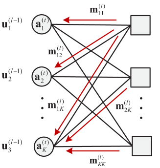
Figure 2: .  Message passing and update for GNNs.

Next, we will elaborate the details of each module in the MPNN, including the propagation, the aggregation, and the readout module.

III-B1 Propagation module

For any pair of variable nodes $x_{n}$ and $x_{j}$, there is an edge to connect them. Each edge first concatenates the connected hidden vectors ${\mathbf{u}}_{n}^{(\ell-1)}$ and ${\mathbf{u}}_{j}^{(\ell-1)}$ with its own attribute $\mathbf{f}_{jn}$ as ${\mathbf{c}}_{n}^{(l-1)}=[{\mathbf{u}}_{n}^{{(}\ell-1{)}},{\mathbf{u}}_{j}^{{(}\ell-1{)}},\mathbf{f}_{jn}]$. Then, it uses the concatenated features ${\mathbf{c}}_{n}^{(l-1)}$ as the input for the multi-layer perceptron (MLP). Therefore, the output of the MLP is given by

$${\mathbf{m}}_{jn}^{(\ell)}={\mathsf{D}}\left({\mathbf{c}}_{n}^{(l-1)}\right),$$ (12)

where $\mathsf{D}$ is the MLP network. In the propagation module, each edge has an MLP with two hidden layers of sizes $N_{h_{1}}$ and $N_{h_{2}}$ and an output layer of size $N_{u}$. Furthermore, the rectifier linear unit (ReLU) activation function is used at the output of each hidden layer. Finally, the outputs ${\mathbf{m}}_{jn}^{(\ell)}$ are fed back to the nodes as shown in Fig. 2.

III-B2 Aggregation module

The $n$-th variable node sums all the incoming messages ${\mathbf{m}}_{jn}^{(\ell)}$ from its connected edges and concatenates the sum of the ${\mathbf{m}}_{jn}^{(\ell)}$ with the node attribute ${\mathbf{a}}_{n}^{(t)}$ as ${\mathbf{m}}_{n}^{(\ell)}=\left[\sum_{\begin{subarray}{c}j=1\\ j\neq n\end{subarray}}^{N}{\mathbf{m}}_{jn}^{(\ell)},{\mathbf{a}}_{n}^{(t)}\right]$. The ${\mathbf{m}}_{n}^{(\ell)}$ is used to compute the node hidden vector ${\mathbf{u}}_{n}^{(\ell)}$ as

$${\mathbf{g}}_{n}^{(\ell)}={\mathsf{U}}\left({\mathbf{g}}_{n}^{(\ell-1)},{\mathbf{m}}_{n}^{(\ell)}\right),$$ (13a)

$${\mathbf{u}}_{n}^{(\ell)}={\mathbf{W}}_{2}\cdot{\mathbf{g}}_{n}^{(\ell)}+{\mathbf{b}}_{2},$$ (13b)

where the function $\mathsf{U}$ is specified by the gated recurrent unit (GRU) network, whose current and previous hidden states are ${\mathbf{g}}_{n}^{(\ell)}\in\mathbb{R}^{N_{h_{1}}}$ and ${\mathbf{g}}_{n}^{({\ell}-1)}\in\mathbb{R}^{N_{h_{1}}}$, respectively. ${\mathbf{W}}_{2}\in\mathbb{R}^{N_{u}\times N_{h_{1}}}$ is a learnable matrix, and ${\mathbf{b}}_{2}\in\mathbb{R}^{N_{u}}$ is a learnable vector. The updated hidden vector (13b) is then sent to the propagation module for next iterations.

III-B3 Readout module

After $L$ rounds of the message passing between the propagation and aggregation module, a readout module is utilized to output the estimated distribution $p_{\mathrm{GNN}}^{(t)}(x_{n}=s_{i}|{\mathbf{y}})$ for the $t$-layer of AMP-GNN and given by

$$\tilde{p}^{(t)}_{\mathrm{GNN}}(x_{n}=s_{i}|{\mathbf{y}})={\mathsf{R}}\left({\mathbf{u}}_{n}^{(L)}\right),s_{i}\in\mathcal{S},$$ (14a)

$$p_{\mathrm{GNN}}^{(t)}(x_{n}=s_{i}|{\mathbf{y}})=\frac{{{\mathsf{e}}{\mathsf{x}}{\mathsf{p}}}\left(\tilde{p}^{(t)}_{G\mathrm{NN}}(x_{n}=s_{i}|{\mathbf{y}})\right)}{\sum_{s_{i}\in\mathcal{S}}{{\mathsf{e}}{\mathsf{x}}{\mathsf{p}}}\left({\tilde{p}}^{(t)}_{\mathrm{GNN}}(x_{n}=s_{i}|{\mathbf{y}})\right)},s_{i}\in\mathcal{S}.$$ (14b)

The readout function ${\mathsf{R}}$ consists of an MLP with two hidden layers of sizes $N_{h_{1}}$ and $N_{h_{2}}$, and ReLU activation is utilized at the output of each hidden layer. The output size of ${\mathsf{R}}$ is the cardinality of the real-valued constellation set, i.e., $\sqrt{Q}$. Then, we compute

$${\mathbf{g}}_{n}^{(0)}\leftarrow{\mathbf{g}}_{n}^{(L)}\text{ and }{\mathbf{u}}_{n}^{(0)}\leftarrow{\mathbf{u}}_{n}^{(L)},n=1,\dots,N,$$ (15)

for the next GNN iteration. Finally, we utilize $p_{\mathrm{GNN}}^{(t)}(x_{n}=s_{i}|{\mathbf{y}})$ to compute the posterior mean and variance for the AMP, which are given by

$$\hat{x}_{n}^{(t+1)}=\mathbb{E}\{x_{n}|p_{\mathrm{GNN}}^{(t)}\},$$ (16a)

$$\hat{v}_{n}^{(t+1)}=\text{Var}\{x_{n}|p_{\mathrm{GNN}}^{(t)}\}.$$ (16b)

Note that the expectation and variance are computed with respect to $p_{\mathrm{GNN}}^{(t)}$. This is the main difference between AMP and AMP-GNN as $p_{\mathrm{GNN}}^{(t)}(x_{n}=s_{i}|{\mathbf{y}})$ is not the Gaussian pdf in the AMP-GNN detector. After computing (16a) and (16b), the posterior mean $\hat{x}_{n}^{(t+1)}$ and $\hat{v}_{n}^{(t+1)}$ will be used for the next AMP-GNN iteration. Finally, the AMP-GNN is executed iteratively until terminated by a fixed number of layers.

TABLE I: Computational complexity (the number of multiplications) of different detectors.

	OAMP-Net	GNN	GEPNet	AMP	AMP-GNN	RE-MIMO
$64\times 64$	$8.22\times 10^{6}$	$1.17\times 10^{6}$	$5.11\times 10^{6}$	$1.78\times 10^{5}$	$2.35\times 10^{6}$	$4.93\times 10^{8}$
$256\times 256$	$5.21\times 10^{8}$	$1.27\times 10^{7}$	$2.02\times 10^{8}$	$2.68\times 10^{6}$	$1.93\times 10^{7}$	$3.22\times 10^{9}$
$1024\times 1024$	$3.33\times 10^{10}$	$5.56\times 10^{8}$	$1.24\times 10^{10}$	$4.22\times 10^{7}$	$6.14\times 10^{8}$	$4.41\times 10^{10}$

III-C Complexity Analysis

We analyze the computational complexity of the AMP-GNN and compare it with existing massive MIMO detectors. Specifically, the complexity of the AMP detector is $\mathcal{O}(MN)$ owing to the matrix-vector multiplication while the complexity for GNN is $\mathcal{O}(N_{h1}N_{h2})$ accounts for the each MLP operation. Therefore, the computational complexity of the AMP-GNN is $\mathcal{O}(MN+NN_{h1}N_{h2})$, dominated by the complexity of the AMP and GNN. In contrast, the complexity of the GEPNet is $\mathcal{O}(M{N}^{2}+NN_{h1}N_{h2})$ which includes the computational complexity of the EP and GNN.

To better compare the complexity, we use the number of multiplication as the metric and show the exact values for different MIMO settings with quadrature phase shift keying (QPSK) symbols in Table. I. The hyperparameters for GNN are set as $N_{h_{1}}=16$, $N_{h_{2}}=8$, and $N_{u}=8$. Compared with state-of-the-art DL-based MIMO detectors, such as GEPNet and RE-MIMO, the AMP-GNN entails a much lower complexity. In particular, the ratio between the complexity of the AMP-GNN and GEPNet is dramatically reduced when the number of user increases. For example, the ratio between the complexity of the AMP-GNN and GEPNet is only $45.99\%$ when $M=N=64$ while the ratio is $4.95\%$ when $M=N=1024$. This is because the complexity of matrix inversion in the GEPNet will be the dominant term, which is prohibitively high when the number of antennas is large. In contrast, the AMP-GNN only involves matrix-vector multiplications, which is a favorable feature for future ultra massive MIMO systems.

IV Simulation Results

In this section, we provide simulation results of the AMP-GNN for massive MIMO detection and compare it with other MIMO detectors. We use the symbol error rate (SER) as the performance metric in our simulations. The signal-to-noise (SNR) of the system, defined as $\mathrm{SNR}=\frac{\mathbb{E}\|\mathbf{H}\mathbf{x}\|^{2}_{2}}{\mathbb{E}\|\mathbf{n}\|^{2}_{2}}$. To illustrate the effectiveness of our proposed AMP-GNN, we adopt several well established MIMO detectors as baselines:

• MMSE: A classical linear receiver for MIMO detection which inverts the received signal by applying the channel-noise regularized pseudo-inverse of the channel matrix.

• AMP: An efficient message passing algorithm for MIMO detection given in Algorithm 1 and implemented with $10$ iterations.

• OAMP-Net: The OAMP-based model-driven DL detector developed in [11]. Each layer requires computing a matrix pseudo-inverse and has 2 learnable parameters.

• EP: The EP-based MIMO detector with 10 iterations as proposed in [3].

• GEPNet: The GNN-enhanced EP detector proposed in [14] with $10$ layers.

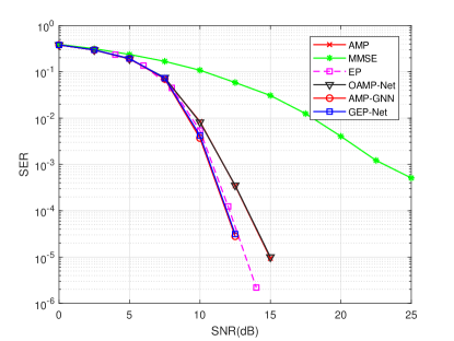
(a) QPSK

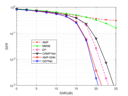
(b) 16-QAM

Figure 3: .  SER comparison of AMP-GNN with other MIMO detectors under $64\times 64$ Rayleigh MIMO channels with QPSK and 16-QAM symbols.

IV-A Implementation Details

In the simulation, the AMP-GNN is implemented on the PyTorch platform. The number of layers of the AMP-GNN detector is set to $T=10$ while the number of layers of the GNN is set to $L=2$. The training data consists of a number of randomly generated pairs $(\mathbf{x},\mathbf{y})$. The data $\mathbf{x}$ is generated from QAM modulation symbols. We train the network with $100$ epochs. At each epoch, the training and validation sets contain $100,000$, and $5,000$ samples, respectively. The AMP-Net is trained using the stochastic gradient descent method and Adam optimizer. The learning rate is set to be $0.001$ and the batch size is set to $64$. We choose the $L_{2}$ loss as the cost function, which is defined by,

$$L_{2}(\mathbf{x},\hat{\mathbf{x}}^{(T)})=\|\mathbf{x}-\hat{\mathbf{x}}^{(T)}\|^{2}.$$ (17)

IV-B Performance Comparsion

Fig. 3 compares the average SER of the AMP-GNN with those of the baseline detectors under $64\times 64$ Rayleigh MIMO channels with QPSK and $16$-QAM symbols, respectively. As can be observed from the figures, the AMP-GNN outperforms almost all other MIMO detectors except for the GEPNet detector. In particular, the AMP-GNN outperforms the AMP detector in all SNRs, which demonstrates the GNN can enhance traditional iterative detector with the help of information from data. Compared with the state-of-the art GEPNet detector, the AMP-GNN can achieve similar performance but with lower complexity. Interestingly, the AMP-GNN can outperform EP detector but with lower complexity, which illustrates the GNN can help to avoid matrix inversion and provide a new thinking for developing message passing algorithms.

IV-C Robustness to Dynamic Numbers of Users

Most of the DL-based MIMO detectors are trained and tested with a fixed number of antennas. However, the number of users in practical MIMO systems may quickly change. For example, new users may access to be served by the BS. As a result, the DL-based MIMO detector should have the ability to handle a varying number of users with a single model. In Fig. 4, we train the AMP-GNN in an $32\times 16$ and $32\times 32$ MIMO systems and test it in a $32\times 24$ MIMO system. As shown in the figure, if we target an $\mathrm{SER}=10^{-3}$, then the AMP-GNN still has $2.0$ dB performance gain compared with the conventional AMP detector even when tested with different number of users. Furthermore, it has a similar performance as the AMP-GNN trained and tested both in the $32\times 24$ MIMO system. As a result, the AMP-GNN has strong robustness to different numbers of users in the deployment stage. This is because the GNN has the permutation equivariance property which makes it robust against the dynamic changes of the number of users.

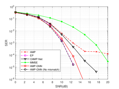
Figure 4: .  Robustness of the AMP-GNN for dynamic number of users.

V Conclusions

We have developed a novel GNN-enhanced AMP detector for massive/ultra-massive MIMO detection, named AMP-GNN, which is obtained by incorporating the GNN module into the AMP algorithm. The AMP-GNN inherits the respective superiority of the low-complexity AMP detector and efficient GNN module. Simulation results demonstrated that AMP-GNN improves the performance of the AMP detector significantly and has comparable performance as the state-of-the-art GEPNet detector but with a reduced computational complexity. Furthermore, it is quite robust to the change of the number of users in practice.

References

- [1] C. Studer, A. Burg, and H. Bölcskei, “Soft-output sphere decoding: algorithms and VLSI implementation,” IEEE J. Sel. Areas Commun., vol. 26, no. 2, pp. 290-300, Feb. 2008.
- [2] S. Wu, L. Kuang, Z. Ni, J. Lu, D. Huang, and Q. Guo, “Low-complexity iterative detection for large-scale multiuser MIMO-OFDM systems using approximate message passing,” IEEE J. Sel. Topics Signal Process., vol. 8, no. 5, pp. 902-915, Oct. 2014.
- [3] J. Céspedes, P. M. Olmos, M. Sánchez-Fern´andez, and F. Pérez-Cruz, “Expectation propagation detection for high-order high-dimensional MIMO systems,” IEEE Trans. Commun., vol. 62, no. 8, pp. 2840-2849, Aug. 2014.
- [4] M. Bayati and A. Montanari, “The dynamics of message passing on dense graphs, with applications to compressed sensing,” IEEE Trans. Inform. Theory, vol. 57, no. 2, pp. 764-785, Feb. 2011.
- [5] T. P. Minka, “A family of algorithms for approximate Bayesian Inference,” Ph.D. dissertation, Dept. Elect. Eng. Comput. Sci., MIT, Cambridge, MA, USA, 2001.
- [6] K. B. Letaief, Y. Shi, J. Lu, and J. Lu, “Edge artificial intelligence for 6G: Vision, enabling technologies, and applications,” IEEE J. Sel. Areas Commun., vol. 40, no. 1, pp. 5-36, 2022.
- [7] K. B. Letaief, W. Chen, Y. Shi, J. Zhang, and Y.-J.-A. Zhang, “The roadmap to 6G: AI-empowered wireless networks,” IEEE Commun. Mag., vol. 57, no. 8, pp. 84-90, Aug. 2019.
- [8] H. He, S. Jin, C.-K. Wen, F. Gao, G. Y. Li, and Z. Xu, “Model-driven deep learning for physical layer communications,” IEEE Wireless Commun., vol. 26, no. 5, pp. 77-83, Oct. 2019.
- [9] H. He, C. K. Wen, S. Jin, and G. Y. Li, “Deep learning-based channel estimation for beamspace mmWave massive MIMO systems,” IEEE Wireless Commun. Lett., vol. 7, no. 5, pp. 852-855, Oct. 2018.
- [10] C.-K. Wen, W. T. Shih, and S. Jin, “Deep learning for massive MIMO CSI feedback,” IEEE Wireless Commun. Lett., vol. 7, no. 5, pp. 748-751, Oct. 2018.
- [11] H. He, C.-K. Wen, S. Jin, and G. Y. Li, “Model-driven deep learning for MIMO detection,” IEEE Trans. Signal Process., vol. 68, pp. 1702-1715, Mar. 2020.
- [12] Y. Shen, J. Zhang, S.H. Song, and K. B. Letaief, “Graph neural networks for wireless communications: From theory to practice,” IEEE Trans. Wireless Commun., early access, doi: 10.1109/TWC.2022.3219840.
- [13] A. Scotti, N. N. Moghadam, D. Liu, K. Gafvert, and J. Huang, “Graph neural networks for massive MIMO detection,” in Proc. Int. Conf. Mach. Learn. (ICML) Workshop, Vienna, Austria, July 2020.
- [14] A. Kosasih et al., “Graph neural network aided expectation propagation detector for MU-MIMO systems,” IEEE J. Sel. Areas Commun., vol. 40, no. 9, pp. 2540-2555, Jul. 2022.
- [15] K. Pratik, B. D. Rao, and M. Welling, “RE-MIMO: Recurrent and permutation equivariant neural MIMO detection,” IEEE Trans. Signal Process., vol. 69, p. 459-473, Jan. 2021.