Calibration of Natural Language Understanding Models with Venn–ABERS Predictors

Abstract

Transformers, currently the state-of-the-art in natural language understanding (NLU) tasks, are prone to generate uncalibrated predictions or extreme probabilities, making the process of taking different decisions based on their output relatively difficult. In this paper we propose to build several inductive Venn–ABERS predictors (IVAP), which are guaranteed to be well calibrated under minimal assumptions, based on a selection of pre-trained transformers. We test their performance over a set of diverse NLU tasks and show that they are capable of producing well-calibrated probabilistic predictions that are uniformly spread over the [0,1] interval – all while retaining the original model’s predictive accuracy.

1 Introduction

Natural language understanding (NLU) systems are rapidly becoming an essential part of many commercial products. A core element in the architecture of any conversational agent, NLU tasks are also behind machine translation, question answering and text classification tasks like sentiment analysis, hate speech detection and fake news detection. Such a shift from the academic realm to a more product-oriented environment was possible because of the recent advancements in natural language processing: massive new datasets, better computing resources, the introduction of pre-training and the transformer resulted in a dramatic performance jump across many tasks.

However, once embedded in a product, any mistake made by the NLU system can result in sub-optimal service, misleading results or even undermine the whole usability of the product (case in point, a faulty speech-to-text engine). In order to mitigate the effects of wrong predictions, NLU systems need the ability to reliably assess their own uncertainty. Mitigation strategies include asking the user for feedback, or even refusing to produce an output, should the model judge its prediction to be too uncertain.

As an example, let us consider a traditional spam detector. Depending on its uncertainty over an incoming message $m$, a spam detector may act in several ways: if the calculated probability of $m$ being spam is $\mathbb{P}(Y=\text{spam}\mid m)=p$, then

• If $p>k_{1}$, where $k_{1}$ is a suitable threshold, say 0.95, send the message to the recycle bin or spam folder

• If $k_{2}<p<k_{1}$, where $k_{2}<k_{1}$ is a lower threshold, ask the user to double check if the message is actually spam

• If $p<k_{2}$ do not take any action.

In order to produce such a behaviour, a model must not only be accurate in detecting spam: it needs to be able to estimate realistic probabilities tailored to each different message, that is, it needs to be well-calibrated and sharp. A well-calibrated model is able to output probabilities that match the observed frequencies of the predicted labels. For example, out of all predictions with an estimated probability of 0.85, exactly 85% of them must be correct predictions.

However, good calibration alone may not be enough: for a test set where spam and not spam are equally frequent, a classifier assigning probability $p=0.50$ to each prediction would indeed be well calibrated, although hardly useful. A sharper model could divide the examples in more than one “category” and assign probabilities accordingly. In the example above, at least 3 categories would be desirable.

In this work we propose to use inductive Venn–ABERS predictors (IVAPs) to build well-calibrated, sharp NLU models. IVAPs have the property of being perfectly calibrated under minimal assumptions. We apply IVAPs to several types of transformer models (Vaswani et al., 2017), a class of pre-trained neural architectures that are currently the state-of-the-art in NLU. Transformers, however, are not guaranteed to be well calibrated and have a strong tendency to output “extreme” probabilities (close to 0 or 1) – hence unable to distinguish any example that lies in between (see fig:roberta-qqp). We show that transformer-based IVAPs are well calibrated and tend to produce a uniform distribution of probability scores: they are sharp in that sense. We test the performance of IVAPs against a range of different NLU tasks which, given the nature of IVAPs, we restrict to the binary case.

The code to reproduce our results is available on GitHub. This includes a link to an interactive Colab notebook.

fig:roberta-qqp

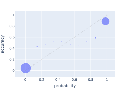
Figure 1: Reliability bubble chart for a RoBERTa model trained on the QQP dataset. The vast majority of predictions are concentrated in only two output probabilities. The few exceptions are grossly uncalibrated.

2 Venn–ABERS predictors

Venn–ABERS predictors (Vovk and Petej, 2014) are a special case of Venn predictors (Vovk et al., 2005), a class of probabilistic predictors guaranteed to be valid under the sole assumption of the training examples being exchangeable. Like all Venn predictors, they need two adjustments to hold their validity guarantee: i) they output multiple probability distributions over the labels – one for each possible label – and ii) their validity property is restricted to perfect calibration. This is because it can be proven that it is impossible to build a valid probabilistic predictor, in the general sense (Gammerman et al., 1998).

Formally, calibration could be defined as follows: let the random variable $Y\in\{0,1\}$ model the label predicted by a binary classifier. Let $P\in[0,1]$ be the confidence associated to the same prediction. $P$ is perfectly calibrated if

$$\mathbb{E}(Y|P)=P$$

almost surely.

Venn–ABERS predictors are binary predictors and output a pair of probabilities $(p_{0},p_{1})$ for each test example $(x,y)$. The former is the probability of $y=1$ should the true label be 0, while the latter is the probability of $y=1$ should the true label be 1: only one of the two is the valid prediction, but we don’t know which one (as we don’t know $y$). Because we always have $p_{0}<p_{1}$, the pair $(p_{0},p_{1})$ can be interpreted as the lower and upper probabilities, respectively, of a certain prediction. Depending on the test example, $p_{0}$ and $p_{1}$ may be more or less different in magnitude, although they are usually close to each other. A large gap between $p_{0}$ and $p_{1}$ signifies low confidence in the probability estimation – something traditional probabilistic predictors are not able to provide. For practical reasons however, it is often useful to have one probability estimate per test example. A reasonable way to combine the two numbers, as explained in Vovk and Petej (2014), is to calculate the probability which minimizes the regret for the log loss function:

$$p=\frac{p_{1}}{1-p_{0}+p_{1}}\>.$$

In this work we will be using the inductive variant of VAPs (IVAP), which was proposed as a computationally lighter version of VAPs in Vovk et al. (2015). This is our only choice as the traditional VAP needs to be retrained for each test example, something absolutely infeasible given the average training time of a transformer model.

IVAPs can be created as follows. Suppose we have a binary classification problem and a scoring algorithm, i.e. any ML algorithm that can issue any confidence score for each prediction – in our case, a transformer model. The general procedure to fit an IVAP is the following:

1. Divide the training set made of examples $(x,y)$ in a proper training set of size $l$ and a calibration set of size $k$

2. Train the transformer on the proper training set

3. Obtain the scores $z_{1},\dots,z_{k}$ for the objects $x_{1},\dots,x_{k}$ in the calibration set

4. For a test example $x$, calculate its score $z$. Fit one isotonic regression on the set $(z_{1},y_{1}),\dots,(z_{k},y_{k}),(z,0)$, then another one on the set $(z_{1},y_{1}),\dots,(z_{k},y_{k}),(z,1)$ so to obtain two functions $f_{0}$ and $f_{1}$.

5. IVAP outputs the multiprobability $(p_{0},p_{1})=(f_{0}(z),f_{1}(z))$

Isotonic regression is a nonparametric form of regression that fits a step-wise, non-decreasing function to a set of examples (see Zadrozny and Elkan, 2002). IVAPs still require for the isotonic regression to be re-calculated for each test example, for each label. Fortunately, Vovk et al. (2015) designed an optimised version that requires a single pre-calculation step ($\mathcal{O}(l\log l)$), then performs an efficient $\mathcal{O}(\log l)$ evaluation step for every test example. We use a Python implementation released by Paolo Toccaceli.

3 Related work

Given the recent developments in the state-of-the-art, the analysis of calibration in NLU tasks (Nguyen and O’Connor, 2015) is gradually turning into the analysis of calibration of transformer models. While Guo et al. (2017) warned about the tendency of “deep” models to produce miscalibrated predictions, Desai and Durrett (2020) and Minderer et al. (2021) showed that recent transformer architectures in particular could be well-calibrated out of the box. However, other studies like the one of Jiang et al. (2021) reported rather poor calibration scores for transformer models on generative question answering datasets. In general, all transformer models seem to benefit from additional calibration steps, and there is no substantial research about their sharpness.

Several recent research contributions focused on building valid predictors to estimate uncertainty in NLU tasks. Mostly based on traditional conformal prediction, models have been built for text classification (Paisios et al., 2019), sentiment analysis (Maltoudoglou et al., 2020), paraphrase detection (Giovannotti and Gammerman, 2021) and part-of-speech tagging and text infilling (Dey et al., 2021). Conformal prediction was also applied to relation extraction (Fisch et al., 2021a) and fact verification (Fisch et al., 2021b).

Venn–ABERS predictors have been successfully applied in different fields, such as drug discovery (Buendia et al., 2019), compound activity prediction (Toccaceli et al., 2016), adversarial manipulation detection (Peck et al., 2020) and log anomaly detection (Pan et al., 2020). To the best of our knowledge, we are the first to apply Venn–ABERS prediction to modelling uncertainty in NLU.

4 Experiments

In this section we provide the details of our experimental process: datasets used, transformer models considered and performance metrics adopted. Because many of these datasets are used in ongoing competitions, their test set labels may be hidden. For these datasets we select the labelled examples and shuffle them into two new training / development sets (see the details in Appendix A).

4.1 Datasets

We tried to include binary datasets that could test our models across different NLU abilities or tasks.

Quora Question Pairs (QQP)

is a large dataset for paraphrase detection: the task of determining if two sentences are semantically equivalent. Each example is a pair of questions taken from those asked on the Quora website. QQP is currently realeased as part of a Kaggle competition.

Stanford Sentiment Treebank (SST)

is a sentiment scoring dataset: each data item is a film review extract labelled with a real number between 0 and 1 that indicates its level of positive sentiment. In our work we transform it into a binary dataset by rounding each label to the nearest integer. SST was introduced by Socher et al. (2013).

Corpus of Linguistic Acceptability (CoLA)

consists of English acceptability judgements drawn from books and journal articles on linguistic theory. Each example is a sequence of words annotated with whether it is a grammatical English sentence. CoLA was introduced in Warstadt et al. (2018) and is currently used in the GLUE public benchmark.

Boolean Questions (BoolQ)

is a question answering dataset for yes/no questions which are naturally occurring – they are generated in unprompted and unconstrained settings. Each example is a triplet of (question, passage, answer). BoolQ was introduced in Clark et al. (2019) and is currently used in the SuperGLUE public benchmark.

4.2 Pre-trained models

Transformer models are rarely trained from scratch, as they are designed to take advantage of large amounts of data and computational resources. Instead, a common practice in ML research is to re-use such pre-trained models by training them again on smaller datasets, which may even model an NLU task different from the one seen at pre-training step. This process, known as fine-tuning, has proven to be beneficial across many benchmarks and allows for the use of powerful models without excessive demands in terms of needed resources.

Following Bowman (2021)’s encouragement to consider more models than just the ubiquitous (and now relatively dated) BERT, we analyse four different pre-trained transformer models to fine-tune on our downstream NLU tasks.

BERT

(Devlin et al., 2019) is arguably the most popular pre-trained large language model, the result of training a transformer over a very large amount of data for two relatively simple NLP tasks. BERT was designed to be adaptable to different prediction types – e.g., regression, span prediction and, as in our case, sequence classification. We use the base-uncased version.

RoBERTa

(Liu et al., 2019) improved on BERT by removing one of the pre-training tasks, modifying key hyperparameters and increasing the size of the training data. We use the roberta-base version.

ALBERT

(Lan et al., 2020) managed to lower memory consumption and increase the training speed of BERT by using two specific parameter-reduction techniques. We use the albert-base-v2 version.

DeBERTa

(He et al., 2021) improves the BERT and RoBERTa models using disentangled attention and enhanced mask decoder on half the size of its predecessors’ training sets. We use version 3 where DeBERTa is further improved using ELECTRA-style pre-training. We use the deberta-v3-small configuration.

4.3 Evaluation metrics

We are primary interested in calibration performance, however we also check predictive performance drops that may occur as a result of the calibration step. Our calibration measure of choice is the expected calibration error, however Appendix B includes definitions and results for two additional measures: log loss and Brier score.

Expected Calibration Error

To compute ECE, all predictions are grouped in $M$ bins of equal width, such that bin $B_{m}$ contains examples with confidence ranging in $(\frac{m-1}{M},\frac{m}{M}]$. ECE is defined as

$$\text{ECE}\coloneqq\frac{1}{n}\sum_{m=1}^{M}|B_{m}|\cdot|p(B_{m})-\hat{p}(B_{m})|$$

where $p(B_{m})$ is the true fraction of positive instances in bin $B_{m}$ and $\hat{p}(B_{m})$ is the average estimated probability for predictions in bin $B_{m}$. For example, an ECE of 0.10 means that on average, the models’ expected probability for a prediction is off by 10%. It is important to note that ECE varies depending on the number of bins $M$: throughout our experiments we will report results for $M=10$.

$F_{1}$ score

Macro-averaged $F_{1}$ score is defined as the arithmetic mean of the $F_{1}$ scores computed for each label. The $F_{1}$ score for a label $k$ is defined as

$$F_{1}^{(k)}=\frac{2P^{(k)}R^{(k)}}{P^{(k)}+R^{(k)}}$$ (1)

where $P$ and $R$ are precision and recall.

Reliability bubble chart

A reliability diagram (see for example Niculescu-Mizil and Caruana, 2005) is a simple line plot that depicts the relationship between output probability and observed frequency (or accuracy, for the binary case). In this work we propose to replace the line plot with a bubble chart: the larger a bubble, the more examples have been assigned that particular probability by the model. Compared to the traditional reliability diagram, a bubble chart shows the model’s preferences in terms of assigning probabilities, allowing for a better grasp of its sharpness.

5 Results

We report results for calibration and predictive accuracy. We include a final experiment where we try to reconstruct SST’s original, real-valued labels from the corresponding binary labels alone.

		QQP	BoolQ	CoLA	SST
ALBERT	default	7.23	7.38	10.30	7.29
	IVAP	0.52	3.32	3.14	3.38
BERT	default	7.46	12.94	10.16	7.15
	IVAP	0.44	3.35	3.09	2.76
DeBERTa	default	6.18	10.79	10.25	4.20
	IVAP	0.48	3.14	2.47	2.39
RoBERTa	default	6.74	10.27	10.48	3.95
	IVAP	0.49	2.79	2.92	2.99

Table 1: Expected calibration error (in %) for default and IVAP models. A lower error means a lower discrepancy between estimated probability and model accuracy.

fig:roberta-ivap-qqp

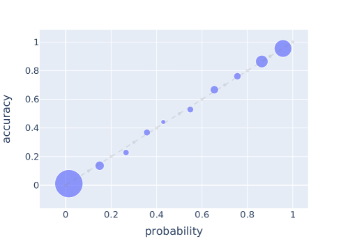
Figure 2: Reliability bubble chart for the IVAP version of RoBERTa trained on the QQP dataset. The model is well-calibrated and the output probabilities are evenly distributed over the [0,1] interval (cfr. fig:roberta-qqp).

5.1 Calibration

tab:ece shows the calibration performance of each transformer model along with its IVAP version. Each IVAP is a clear improvement over its original counterpart in terms of ECE. We notice how QQP, by far the largest of the 4 datasets, seems to attract better results: IVAPs are all almost perfectly calibrated ($\text{ECE}\sim 0.005$). This may be due to the size of QQP’s calibration set. As for the other three tasks, IVAPs still manage to reduce a model’s ECE to 1/3 of the original, on average.

Among the four transformers, there is no dramatic difference between large (RoBERTa, DeBERTa) and smaller (BERT, ALBERT) models, even if the former actually manage to score better in 2 out of 4 tasks. Larger models however do benefit the most from being transformed into IVAP: the best calibration scores for IVAPs are shared between RoBERTa and DeBERTa.

For a more complete reporting of the calibration results, we include log loss and Brier scores in Appendix B.

By inspecting the reliability bubble charts, it is evident how IVAPs are sharper than their original counterparts: as fig:roberta-ivap-qqp shows, IVAP’s probability scores are distributed relatively evenly over the [0,1] interval (compare with fig:roberta-qqp).

As a final note, we report that IVAP calibration scores are more reliable, in the sense that they show a lower variability. For example, ECE for IVAPs never exceeds 5% whereas it can vary from 1% to 15% among default models (see fig:ECEdist in Appendix C).

5.2 Predictive accuracy

Our main interest about predictive accuracy is to check if using IVAP – and its reduced training set – can harm the original model performance. tab:f1 shows that there is a slight tendency of IVAP models to lose about 1% $F_{1}$ score over their default version; however, this tendency wears off as the default model’s performance increases, while sometimes IVAP can actually score even better (see RoBERTa on CoLA and SST).

In general, we note that while larger transformer models consistently achieve better scores than smaller ones, the gap in performance seem to become narrower for bigger datasets (see QQP).

Finally, the general trend is that more accurate models achieve better calibration (see fig:ECEvsF1 in Appendix C).

		QQP	BoolQ	CoLA	SST
ALBERT	default	0.90	0.70	0.79	0.87
	IVAP	0.90	0.68	0.77	0.86
BERT	default	0.90	0.69	0.80	0.87
	IVAP	0.90	0.69	0.78	0.86
DeBERTa	default	0.91	0.77	0.84	0.89
	IVAP	0.91	0.76	0.83	0.89
RoBERTa	default	0.91	0.77	0.81	0.89
	IVAP	0.90	0.75	0.82	0.90

Table 2: Classification performance: $F_{1}$ scores for default and IVAP models.

5.3 Estimating the degree of positive sentiment

Some classification tasks are “more binary” than others: label sets like $\mathcal{Y}=\{\text{alive},\text{dead}\}$ define unambiguously a certain aspect of an object. However, binary labels may hide a more nuanced separation of the examples – this is often the case of sentiment analysis. Because human sentiment is so subjective, it is hard to devise a labelling strategy that preserves the more subtle aspects of it, even (or maybe especially) in the simple case of $\mathcal{Y}=\{\text{negative, positive}\}$.

The Stanford Sentiment Treebank (SST, see Section 4.1), addresses this problem by assigning each example a real number $y\in[0,1]$ representing the degree of positive sentiment of the sentence. In this work, we rounded those labels to the nearest integer to shape our task into binary sentiment analysis. This has already been done before, for example in the GLUE benchmark.

However, given the nature of the problem, and that on paper the aim of NLU should be “understanding” language, we think it would be preferable to build models that estimate uncertainty like humans do. Certainly, we can fit a simple regression model to predict SST’s real-valued labels, but what if only binary labels were provided at training time? Would the probabilities generated by a model resemble the degree of human confidence in assigning a postive sentiment label?

As it turns out, the distribution of probability scores issued by NLU models doesn’t really match that of confidence scores as judged by humans (see fig:prob_dist in Appendix C). Nonetheless, IVAP models (and, we suspect, all well-calibrated and sharp models) manage to mimic human judgement in a better way. We compared the numeric labels in SST with the probabilities estimated by our transformer models and their IVAP variant. In tab:r2 we show root mean squared error (RMSE) and $R^{2}$ score calculated over ground-truth and estimated degrees of positive sentiment. It is easy to verify how IVAPs always manage to achieve a better match of the human scores compared to their default counterparts.

		RMSE	$R^{2}$
ALBERT	default	0.28	-0.22
	IVAP	0.22	0.25
BERT	default	0.29	-0.27
	IVAP	0.23	0.23
DeBERTa	default	0.25	0.01
	IVAP	0.23	0.20
RoBERTa	default	0.26	-0.05
	IVAP	0.22	0.25

Table 3: Estimation of the degree of positive sentiment in SST, when only binary labels are supplied at training time. Model’s probabilities are compared to ground-truth labels in SST (lower RMSE and higher $R^{2}$ are better).

6 Conclusion

We showed that Venn–ABERS predictors can be successfully applied to transformer models to obtain well-calibrated predictions for natural language understanding tasks. IVAPs were particularly effective when trained on a large dataset ($\text{ECE}<1\%$) and retained the classification accuracy of original transformer models. Moreover, IVAPs showed to be sharper: output probabilities were more evenly distributed in the $[0,1]$ interval and less condensed around a single value.

We restricted our experiments to the binary case, which is an obvious simplification of many real-world scenarios (e.g., detection of multiple intents in a chatbot, multiple topics of a message). However, Manokhin (2017) and Johansson et al. (2021) both introduced methods to extend IVAPs to the multiclass case. This would allow us to directly compare Venn–ABERS to another calibration technique which is gaining traction in the deep learning community especially: temperature scaling (Guo et al., 2017).

In terms of NLU, we avoided tasks like open question answering, machine translation and text summarization (all generative tasks). Because there is not a single label $y$ for each example – rather, a very large and potentially infinite set of possible labels – an entire new and more useful definition for calibration may be needed.

The need for reliable NLU models will continue to grow as cutting-edge research is transformed into products for large audiences: users need to know when to trust a certain output. In a broader sense, we may say that a system with the ability of assessing its own uncertainty will always feel more “intelligent” than a blindly overconfident one. This reinforces the need for accurate calibration on the path towards a better AI.

Appendix A Experimental setup

All datasets except SST have hidden test sets as they are being used in ongoing competitions. For our experiments we concatenate their training and validation sets, shuffle the resulting dataset and split it again in training, validation and test set. For the IVAP training we further split each training set into 75% proper training set and 15% calibration set. The dataset sizes are summarized in tab:splits.

Because transformers are known to display some degree of variability in performance depending on the initial seed (Mosbach et al., 2021), we run 5 training trials and average their scores for all datasets, with the exception of QQP. In some occasions, a model would get stuck in a local minimum and perform extremely poorly – this occurrences were removed from the calculation of the average as they would have skewed the result unnaturally.

All models were trained for 3 epochs with a learning rate of $2\cdot 10^{-5}$ using the AdamW optimizer (Loshchilov and Hutter, 2019).

Training was performed on a single NVidia V100 hosted on the AWS platform.

	QQP	BoolQ	CoLA	SST
Train	323,416	9,427	7,468	8,544
Validation	40,430	1,635	1,063	1,101
Test	40,430	1,635	1,063	2,210

Table 4: Size of train, validation and test splits for the 4 datasets.

Appendix B Additional calibration measures

We include results for calibration performance measured by log loss and Brier score, all averaged over 5 trials as detailed in Appendix A.

Log loss, or cross-entropy loss, is based on how much a prediction with probability $p=\mathbb{P}(y=1)$ differs from the real label $y\in\{0,1\}$. It is defined as

$$L(y,p)=-(y\log p+(1-y)\log(1-p))$$

Intuitively, the lower the log loss averaged over the test set, the better a model is calibrated. Results of all models are summarised in tab:logloss.

Brier score is the mean squared error of the predictions over the test set, i.e.:

$$L_{B}=\frac{1}{N}\sum_{i=1}^{N}(p_{i}-y_{i})^{2}$$

Unlike log loss, Brier score does not implode to $-\infty$ when a wrong prediction is given with $p=0$ or $p=1$. Results of all models are summarised in tab:brier.

		QQP	BoolQ	CoLA	SST
ALBERT	default	0.34	0.55	0.49	0.38
	IVAP	0.24	0.54	0.41	0.32
BERT	default	0.35	0.63	0.51	0.38
	IVAP	0.23	0.55	0.40	0.32
DeBERTa	default	0.29	0.53	0.49	0.29
	IVAP	0.21	0.46	0.33	0.26
RoBERTa	default	0.31	0.52	0.49	0.28
	IVAP	0.22	0.47	0.36	0.27

Table 5: Log loss results for default and IVAP models.

		QQP	BoolQ	CoLA	SST
ALBERT	default	0.082	0.182	0.137	0.103
	IVAP	0.072	0.182	0.127	0.099
BERT	default	0.081	0.206	0.129	0.107
	IVAP	0.068	0.184	0.122	0.097
DeBERTa	default	0.072	0.161	0.113	0.081
	IVAP	0.064	0.150	0.098	0.078
RoBERTa	default	0.076	0.159	0.123	0.082
	IVAP	0.067	0.154	0.109	0.078

Table 6: Brier scores for default and IVAP models.

Appendix C Additional plots

fig:ECEdist shows how IVAP models are more consistently calibrated regardless of the initial seed used for model generation. On the other hand, default models can be more or less well-calibrated, depending on how “lucky” the initial seed is.

fig:ECEvsF1 shows that more accurate models tend to be better calibrated. However, this tendency is attenuated when using IVAP models.

fig:prob_dist shows the distribution of human scores in the SST dataset, together with IVAP’s and the default model’s estimations. IVAP tries to recreate the essentially bimodal distribution of human scores, while the default model (in this case a fine-tuned DeBERTa) struggles to do so and prefers extreme values of probability.

fig:ECEdist

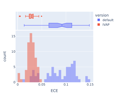
Figure 3: Distribution of expected calibration errors over all datasets, models and trials.

fig:ECEvsF1

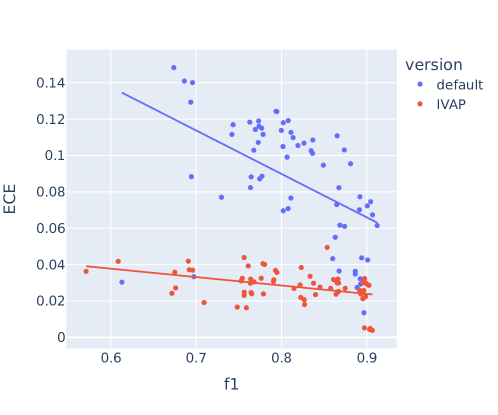
Figure 4: Trend of expected calibration error versus $F_{1}$ score for all models and datasets.

fig:prob_dist

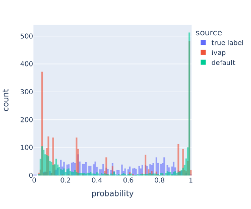
Figure 5: Distribution of ground-truth scores in SST, compared to IVAP’s and default model’s estimations.

References

- Bowman (2021) Samuel R Bowman. When combating hype, proceed with caution. arXiv preprint arXiv:2110.08300, 2021.
- Buendia et al. (2019) Ruben Buendia, Thierry Kogej, Ola Engkvist, Lars Carlsson, Henrik Linusson, Ulf Johansson, Paolo Toccaceli, and Ernst Ahlberg. Accurate hit estimation for iterative screening using venn–abers predictors. Journal of Chemical Information and Modeling, 59(3):1230–1237, 2019.
- Clark et al. (2019) Christopher Clark, Kenton Lee, Ming-Wei Chang, Tom Kwiatkowski, Michael Collins, and Kristina Toutanova. BoolQ: Exploring the surprising difficulty of natural yes/no questions. In Proceedings of the 2019 Conference of the North American Chapter of the Association for Computational Linguistics: Human Language Technologies, Volume 1 (Long and Short Papers), pages 2924–2936, Minneapolis, Minnesota, June 2019. Association for Computational Linguistics. 10.18653/v1/N19-1300. URL https://aclanthology.org/N19-1300.
- Desai and Durrett (2020) Shrey Desai and Greg Durrett. Calibration of pre-trained transformers. In Proceedings of the 2020 Conference on Empirical Methods in Natural Language Processing (EMNLP), pages 295–302, Online, November 2020. Association for Computational Linguistics. 10.18653/v1/2020.emnlp-main.21. URL https://www.aclweb.org/anthology/2020.emnlp-main.21.
- Devlin et al. (2019) Jacob Devlin, Ming-Wei Chang, Kenton Lee, and Kristina Toutanova. BERT: Pre-training of deep bidirectional transformers for language understanding. In Proceedings of the 2019 Conference of the North American Chapter of the Association for Computational Linguistics: Human Language Technologies, Volume 1 (Long and Short Papers), pages 4171–4186, Minneapolis, Minnesota, June 2019. Association for Computational Linguistics. 10.18653/v1/N19-1423. URL https://www.aclweb.org/anthology/N19-1423.
- Dey et al. (2021) Neil Dey, Jing Ding, Jack Ferrell, Carolina Kapper, Maxwell Lovig, Emiliano Planchon, and Jonathan P Williams. Conformal prediction for text infilling and part-of-speech prediction. arXiv preprint arXiv:2111.02592, 2021.
- Fisch et al. (2021a) Adam Fisch, Tal Schuster, Tommi Jaakkola, and Dr.Regina Barzilay. Few-shot conformal prediction with auxiliary tasks. In Marina Meila and Tong Zhang, editors, Proceedings of the 38th International Conference on Machine Learning, volume 139 of Proceedings of Machine Learning Research, pages 3329–3339. PMLR, 18–24 Jul 2021a. URL https://proceedings.mlr.press/v139/fisch21a.html.
- Fisch et al. (2021b) Adam Fisch, Tal Schuster, Tommi S. Jaakkola, and Regina Barzilay. Efficient conformal prediction via cascaded inference with expanded admission. In International Conference on Learning Representations, 2021b. URL https://openreview.net/forum?id=tnSo6VRLmT.
- Gammerman et al. (1998) A. Gammerman, V. Vovk, and V. Vapnik. Learning by transduction. In Proceedings of the Fourteenth Conference on Uncertainty in Artificial Intelligence, UAI’98, page 148–155, San Francisco, CA, USA, 1998. Morgan Kaufmann Publishers Inc. ISBN 155860555X.
- Giovannotti and Gammerman (2021) Patrizio Giovannotti and Alex Gammerman. Transformer-based conformal predictors for paraphrase detection. In Lars Carlsson, Zhiyuan Luo, Giovanni Cherubin, and Khuong An Nguyen, editors, Proceedings of the Tenth Symposium on Conformal and Probabilistic Prediction and Applications, volume 152 of Proceedings of Machine Learning Research, pages 243–265. PMLR, 08–10 Sep 2021. URL https://proceedings.mlr.press/v152/giovannotti21a.html.
- Guo et al. (2017) Chuan Guo, Geoff Pleiss, Yu Sun, and Kilian Q. Weinberger. On calibration of modern neural networks. In Proceedings of the 34th International Conference on Machine Learning, volume 70 of Proceedings of Machine Learning Research, pages 1321–1330, International Convention Centre, Sydney, Australia, 06–11 Aug 2017. PMLR. URL http://proceedings.mlr.press/v70/guo17a.html.
- He et al. (2021) Pengcheng He, Xiaodong Liu, Jianfeng Gao, and Weizhu Chen. {DEBERTA}: {DECODING}-{enhanced} {bert} {with} {disentangled} {attention}. In International Conference on Learning Representations, 2021. URL https://openreview.net/forum?id=XPZIaotutsD.
- Jiang et al. (2021) Zhengbao Jiang, Jun Araki, Haibo Ding, and Graham Neubig. How Can We Know When Language Models Know? On the Calibration of Language Models for Question Answering. Transactions of the Association for Computational Linguistics, 9:962–977, 09 2021. ISSN 2307-387X. 10.1162/tacl_a_00407. URL https://doi.org/10.1162/tacl_a_00407.
- Johansson et al. (2021) Ulf Johansson, Tuwe Löfström, and Henrik Boström. Calibrating multi-class models. In Lars Carlsson, Zhiyuan Luo, Giovanni Cherubin, and Khuong An Nguyen, editors, Proceedings of the Tenth Symposium on Conformal and Probabilistic Prediction and Applications, volume 152 of Proceedings of Machine Learning Research, pages 111–130. PMLR, 08–10 Sep 2021. URL https://proceedings.mlr.press/v152/johansson21a.html.
- Lan et al. (2020) Zhenzhong Lan, Mingda Chen, Sebastian Goodman, Kevin Gimpel, Piyush Sharma, and Radu Soricut. Albert: A lite bert for self-supervised learning of language representations. In International Conference on Learning Representations, 2020. URL https://openreview.net/forum?id=H1eA7AEtvS.
- Liu et al. (2019) Yinhan Liu, Myle Ott, Naman Goyal, Jingfei Du, Mandar Joshi, Danqi Chen, Omer Levy, Mike Lewis, Luke Zettlemoyer, and Veselin Stoyanov. Roberta: A robustly optimized bert pretraining approach. arXiv preprint arXiv:1907.11692, 2019.
- Loshchilov and Hutter (2019) Ilya Loshchilov and Frank Hutter. Decoupled weight decay regularization. In International Conference on Learning Representations, 2019. URL https://openreview.net/forum?id=Bkg6RiCqY7.
- Maltoudoglou et al. (2020) Lysimachos Maltoudoglou, Andreas Paisios, and Harris Papadopoulos. Bert-based conformal predictor for sentiment analysis. volume 128 of Proceedings of Machine Learning Research, pages 269–284. PMLR, 09–11 Sep 2020. URL http://proceedings.mlr.press/v128/maltoudoglou20a.html.
- Manokhin (2017) Valery Manokhin. Multi-class probabilistic classification using inductive and cross Venn–Abers predictors. In Alex Gammerman, Vladimir Vovk, Zhiyuan Luo, and Harris Papadopoulos, editors, Proceedings of the Sixth Workshop on Conformal and Probabilistic Prediction and Applications, volume 60 of Proceedings of Machine Learning Research, pages 228–240. PMLR, 13–16 Jun 2017. URL https://proceedings.mlr.press/v60/manokhin17a.html.
- Minderer et al. (2021) Matthias Minderer, Josip Djolonga, Rob Romijnders, Frances Hubis, Xiaohua Zhai, Neil Houlsby, Dustin Tran, and Mario Lucic. Revisiting the calibration of modern neural networks. Advances in Neural Information Processing Systems, 34, 2021.
- Mosbach et al. (2021) Marius Mosbach, Maksym Andriushchenko, and Dietrich Klakow. On the stability of fine-tuning {bert}: Misconceptions, explanations, and strong baselines. In International Conference on Learning Representations, 2021. URL https://openreview.net/forum?id=nzpLWnVAyah.
- Nguyen and O’Connor (2015) Khanh Nguyen and Brendan O’Connor. Posterior calibration and exploratory analysis for natural language processing models. In Proceedings of the 2015 Conference on Empirical Methods in Natural Language Processing, pages 1587–1598, Lisbon, Portugal, September 2015. Association for Computational Linguistics. 10.18653/v1/D15-1182. URL https://aclanthology.org/D15-1182.
- Niculescu-Mizil and Caruana (2005) Alexandru Niculescu-Mizil and Rich Caruana. Predicting good probabilities with supervised learning. In Proceedings of the 22nd international conference on Machine learning, pages 625–632, 2005.
- Paisios et al. (2019) Andreas Paisios, Ladislav Lenc, Jiří Martínek, Pavel Král, and Harris Papadopoulos. A deep neural network conformal predictor for multi-label text classification. volume 105 of Proceedings of Machine Learning Research, pages 228–245, Golden Sands, Bulgaria, 09–11 Sep 2019. PMLR. URL http://proceedings.mlr.press/v105/paisios19a.html.
- Pan et al. (2020) Lanlan Pan, Zhaojun Gu, Yitong Ren, Chunbo Liu, and Zhi Wang. An anomaly detection method for system logs using venn-abers predictors. In 2020 IEEE Fifth International Conference on Data Science in Cyberspace (DSC), pages 362–368. IEEE, 2020.
- Peck et al. (2020) Jonathan Peck, Bart Goossens, and Yvan Saeys. Detecting adversarial manipulation using inductive venn-abers predictors. Neurocomputing, 2020.
- Socher et al. (2013) Richard Socher, Alex Perelygin, Jean Wu, Jason Chuang, Christopher D. Manning, Andrew Ng, and Christopher Potts. Recursive deep models for semantic compositionality over a sentiment treebank. In Proceedings of the 2013 Conference on Empirical Methods in Natural Language Processing, pages 1631–1642, Seattle, Washington, USA, October 2013. Association for Computational Linguistics. URL https://www.aclweb.org/anthology/D13-1170.
- Toccaceli et al. (2016) Paolo Toccaceli, Ilia Nouretdinov, Zhiyuan Luo, Vladimir Vovk, Lars Carlsson, and Alex Gammerman. Excape wp1. probabilistic prediction, 2016.
- Vaswani et al. (2017) Ashish Vaswani, Noam Shazeer, Niki Parmar, Jakob Uszkoreit, Llion Jones, Aidan N Gomez, Ł ukasz Kaiser, and Illia Polosukhin. Attention is all you need. In I. Guyon, U. V. Luxburg, S. Bengio, H. Wallach, R. Fergus, S. Vishwanathan, and R. Garnett, editors, Advances in Neural Information Processing Systems, volume 30. Curran Associates, Inc., 2017. URL https://proceedings.neurips.cc/paper/2017/file/3f5ee243547dee91fbd053c1c4a845aa-Paper.pdf.
- Vovk and Petej (2014) V. Vovk and Ivan Petej. Venn-abers predictors. In UAI, 2014. URL http://alrw.net/articles/07.pdf.
- Vovk et al. (2005) Vladimir Vovk, Alex Gammerman, and Glenn Shafer. Algorithmic learning in a random world. Springer Science & Business Media, 2005. https://doi.org/10.1007/b106715.
- Vovk et al. (2015) Vladimir Vovk, Ivan Petej, and Valentina Fedorova. Large-scale probabilistic predictors with and without guarantees of validity. In Advances in Neural Information Processing Systems, pages 892–900, 2015.
- Warstadt et al. (2018) Alex Warstadt, Amanpreet Singh, and Samuel R Bowman. Neural network acceptability judgments. arXiv preprint arXiv:1805.12471, 2018.
- Zadrozny and Elkan (2002) Bianca Zadrozny and Charles Elkan. Transforming classifier scores into accurate multiclass probability estimates. In Proceedings of the eighth ACM SIGKDD international conference on Knowledge discovery and data mining, pages 694–699, 2002.