Part I

Long, long ago, in a galaxy far, far away…

The following is the author’s PhD Thesis, defended in September 2017. It has not been edited since (except for the footnotes in the open problems section and for this note). In particular, there is nothing here about applications of Białynicki-Birula decomposition to Hilbert schemes [Jel19, Jel20, SS21], the multigraded Hilbert schemes and border apolarity [BB21, Mań20], fiber-full Hilbert schemes [CRR21, CRR22] and other recent developments. Philosophically speaking, is it reassuring that there are too many new interesting papers on Hilbert schemes of points to summarize here. It is also very interesting that many of the open problems listed below in §1.5 remain actual. Today, the author would add also the more applied open problems (see [JLP22]): a large part of the classical problem of determining the complexity of matrix multiplication can be reduced fruitfully to the study of the Hilbert scheme of points.

While the author is not aware of any errors, it is likely they exist here. This work is put on arXiv due/thanks to several people who decided to refer to it and only to grant this piece a quasi-permanent place to rest.

University of Warsaw

Faculty of Mathematics, Informatics and Mechanics

Joachim Jelisiejew

Hilbert schemes of points and their applications

PhD dissertation

Supervisor

dr hab. Jarosław Buczyński

Institute of Mathematics

University of Warsaw

and Institute of Mathematics

Polish Academy of Sciences

Auxiliary Supervisor
dr Weronika Buczyńska
Institute of Mathematics
University of Warsaw

m

Author’s declaration:

I hereby declare that I have written this dissertation myself and all the contents of the dissertation have been obtained by legal means.

May 9, 2017       ……………………………………………

Joachim Jelisiejew

Supervisors’ declaration:

The dissertation is ready to be reviewed.

May 9, 2017       ……………………………………………

dr hab. Jarosław Buczyński

May 9, 2017      ……………………………………………

dr Weronika Buczyńska

m

Abstract

This thesis is concerned with deformation theory of finite subschemes of smooth varieties. Of central interest are the smoothable subschemes (i.e., limits of smooth subschemes). We prove that all Gorenstein subschemes of degree up to $13$ are smoothable. This result has immediate applications to finding equations of secant varieties. We also give a description of nonsmoothable Gorenstein subschemes of degree $14$, together with an explicit condition for smoothability.

We prove that being smoothable is a local property, that it does not depend on the embedding and it is invariant under a base field extension. The above results are equivalently stated in terms of the Hilbert scheme of points, which is the moduli space for this deformation problem.

We extensively use the combinatorial framework of Macaulay’s inverse systems. We enrich it with a pro-algebraic group action and use this to reprove and extend recent classification results by Elias and Rossi. We provide a relative version of this framework and use it to give a local description of the universal family over the Hilbert scheme of points.

We shortly discuss history of Hilbert schemes of points and provide a list of open questions.

Keywords: deformation theory, Hilbert scheme, Gorenstein algebra, inverse system, apolarity, smoothability, classification of finite commutative algebras.

AMS MSC 2010 classification: 14C05, 14B07, 13N10, 13H10.

Contents

1. I
   1. 1 Introduction
      1. 1.1 Overview and main results
      2. 1.2 Application to secant varieties
      3. 1.3 Application to constructing $r$-regular maps
      4. 1.4 A brief historical survey
      5. 1.5 Open problems
2. II Finite algebras
   1. 2 Basic properties of finite algebras
      1. 2.1 Gorenstein algebras
      2. 2.2 Hilbert function of a local algebra
      3. 2.3 Hilbert function of a local Gorenstein algebra
      4. 2.4 Betti tables, Boij and Söderberg theory
   2. 3 Macaulay’s inverse systems (apolarity)
      1. 3.1 Definition of contraction action
      2. 3.2 Automorphisms and derivations of the power series ring
      3. 3.3 Classification of local embedded Gorenstein algebras via apolarity
      4. 3.4 Hilbert functions of Gorenstein algebras in terms of inverse systems
      5. 3.5 Standard forms of dual generators
      6. 3.6 Simplifying dual generators
      7. 3.7 Examples I — compressed algebras
      8. 3.8 Examples II — $(1,3,3,3,1)$
      9. 3.9 Examples III — preliminaries for Chapter 6
3. III Hilbert schemes
   1. 4 Preliminaries
      1. 4.1 Moduli spaces of finite algebras, Hilbert schemes
      2. 4.2 Base change of Hilbert schemes
      3. 4.3 Loci of Hilbert schemes of points
      4. 4.4 Relative Macaulay’s inverse systems
      5. 4.5 Homogeneous forms and secant varieties
   2. 5 Smoothings
      1. 5.1 Abstract smoothings
      2. 5.2 Comparing abstract and embedded smoothings
      3. 5.3 Embedded smoothability depends only on singularity type
      4. 5.4 Comparing embedded smoothings and the Hilbert scheme
      5. 5.5 Smoothings over rational curves
      6. 5.6 Examples of nonsmoothable finite schemes
      7. 5.7 Example of smoothings: one-dimensional torus limits
4. IV Applications
   1. 6 Gorenstein loci for small number of points
      1. 6.1 Ray families
      2. 6.2 Ray families from Macaulay’s inverse systems.
      3. 6.3 Tangent preserving ray families
      4. 6.4 Proof of Theorem 6.1 — preliminaries
      5. 6.5 Proof of Theorem 6.1 — smoothability results
      6. 6.6 Proof of Theorem 6.3 — the nonsmoothable component (1,6,6,1)
   2. 7 Small punctual Hilbert schemes

Chapter 1 Introduction

The Hilbert scheme of points on a smooth variety $X$ is of central interest for several branches of mathematics:

• in commutative algebra, it is a moduli space of finite algebras (presented as quotients of a fixed ring),

• in geometry and topology, it is a compact variety containing the space of tuples of points on $X$; in many cases this space is dense,

• in algebraic geometry, its construction (1960-61) is one of the advances of the Grothendieck school [Gro95], it found applications in constructing other moduli spaces and hyperkähler manifolds, and also in McKay correspondence and theory of higher secant varieties,

• in combinatorics, the Hilbert scheme appears in Haiman’s proofs of $n!$ and Macdonald positivity conjectures.

Consider the set of finite algebras, presented as quotients of a fixed polynomial ring. There is a unique and natural topological space structure on this set, together with a sheaf of regular functions. These structures jointly give a scheme structure, called the Hilbert scheme of points on affine space, see Chapter 4.1 for precise definition. These structures are unique, but they are non-explicit and difficult to investigate; many open questions persist, despite continuous research, see Section 1.5.

In this thesis we analyse the geometry of Hilbert schemes of points on smooth varieties, concentrating on the following question:

What are the irreducible components of the Hilbert scheme of points? What are their intersections and singularities?

An informal, intuitive view of geometry of the components is given on Figure 1.1 below.

Our analysis of the Hilbert scheme as a moduli space of finite algebras requires tools for working with algebras themselves, which are developed in Part II. We then switch our attention to families of algebras (subschemes) in Part III and analyse Hilbert schemes for small numbers of points in Part IV. Almost all of our original results presented in this thesis are also found in [Jel14, CJN15, Jel18, BJ17, Jel17, BJJMe19].

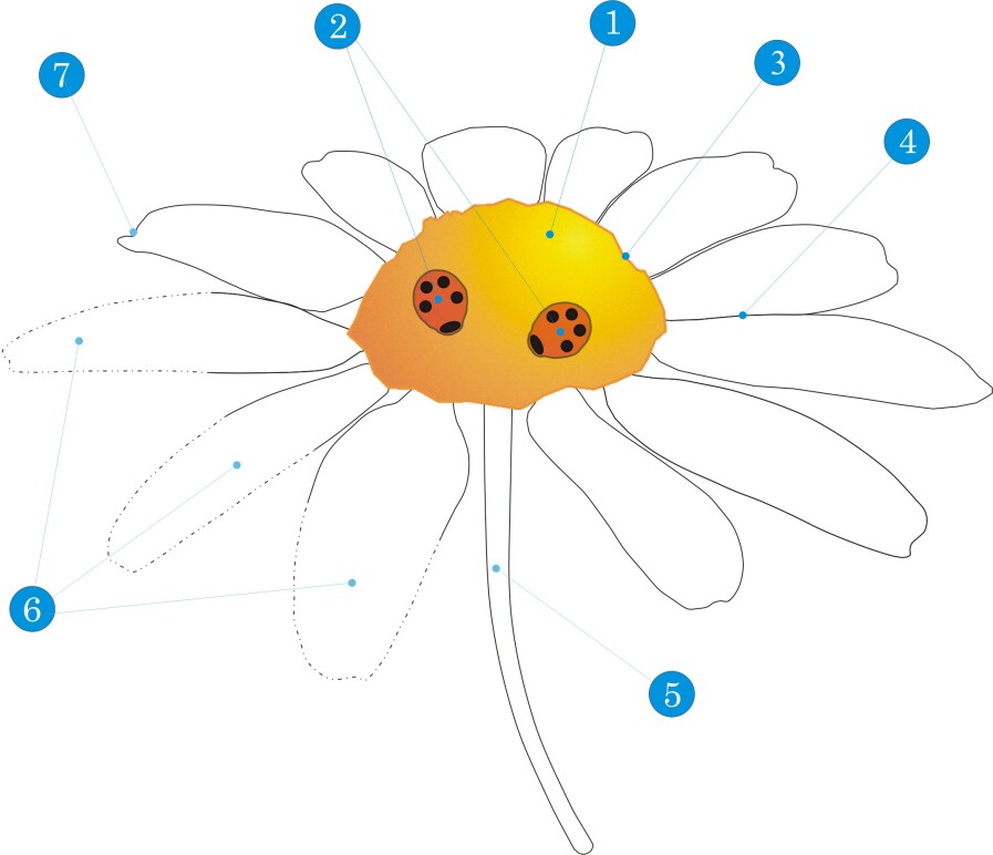
Figure 1.1: Bellis Hilbertis. Components of the Hilbert scheme of $r$ points on a smooth variety $X$. Flower, petals and stem correspond to irreducible components of the Hilbert scheme of $X$. The analysis of their geometry is the main aim of this work.

1. 
   

   The smoothable component, see Definition 4.23. It compactifies the space of $r$-tuples of points on $X$, thus has dimension $r(\dim X)$. For small $r$, it is the only component – there are no “petals” – see Section 5.6, Theorem 6.1 and also Problems 1.16, 1.17.

2. 
   

   Points of the Hilbert scheme correspond to finite subschemes of $X$. General points on the smoothable component (“ladybirds”) correspond to tuples of points on $X$. Thus all subschemes corresponding to points on this component are limits of tuples of points; they are smoothable.

3. 
   

   Every component intersects the smoothable one, see [Ree95]. Describing the intersection is subtle, see Problem 1.19 and Theorem 6.3 for an example involving cubic fourfolds. It is even hard to decide whether a given subscheme of $X$ is smoothable, see Problem 1.18.

4. 
   

   There is a single example [EV10], where components intersect away from the smoothable component. No singular points lying on a unique nonsmoothable component are known.

5. 
   

   There are only few known components of dimension smaller than the smoothable one, see Section 5.6 and Problems 1.22, 1.23.

6. 
   

   There are many examples of loci too large to fit inside the smoothable component, see Section 5.6, however the components containing these loci are not known.

7. 
   

   Not much is known about the geometry and singularities of components other than the smoothable one, see Problem 1.13, Problem 1.14.

1.1 Overview and main results

Part II gathers tools for studying finite local algebras over a field $\Bbbk$, especially Gorenstein algebras. In this part, we speak the language of algebra; only basic background on commutative algebras and Lie theory is assumed. Part II is mostly prerequisite, although Sections 3.5-3.9 contain many original results published in [BJMMR18, Jel17].

Theory of Macaulay’s inverse systems (also known as apolarity) is a central tool in our investigation. To an element $f$ of a (divided power) polynomial ring $P$ it assigns a finite local Gorenstein algebra $\operatorname{Apolar}\left(f\right)$, see Section 3.3. A pro-algebraic group $\mathbb{G}$ acts on $P$ so that the orbits are isomorphism classes of $\operatorname{Apolar}\left(-\right)$, see Section 3.3. In Section 3.6 we explicitly describe the action of $\mathbb{G}$ and investigate its Lie group, building an effective tool to investigate isomorphism classes of algebras. We then give applications; as a sample result, we reprove (with weaker assumptions on the base field) the following main theorems of [ER12, ER15].

Theorem 1.1 (Example 3.35, Corollary 3.73).

Let $\Bbbk$ be a field of characteristic $\neq 2,3$. Let $(A,\mathfrak{m},\Bbbk)$ be a finite Gorenstein local $\Bbbk$-algebra with Hilbert function $(1,n,n,1)$ or $(1,n,\binom{n+1}{2},n,1)$. Then $A$ isomorphic to its associated graded algebra $\operatorname{gr}A$.

Interestingly, Theorem 1.1 fails for small characteristics, see Example 3.74. We also obtain genuine, down to earth classification results, such as the following.

Proposition 1.2 (Example 3.75).

Let $\Bbbk$ be an algebraically closed field of characteristic $\neq 2,3$. There are exactly eleven isomorphism types of finite local Gorenstein algebras with Hilbert function $(1,3,3,3,1)$, see Example 3.75 for their list.

In Part III, our attention shifts towards families of algebras. Accordingly, we change the language from algebra to algebraic geometry, from finite algebras to finite schemes. The main object is the Hilbert scheme of points on a scheme $X$, denoted by $\mathcal{H}\mathit{ilb\/}{}_{r}\,(X)$, together with its degree $r$ finite flat universal family

$$\pi\colon\mathcal{U}\to\mathcal{H}\mathit{ilb\/}{}_{r}\,(X).$$

Intuitively, points of $\mathcal{H}\mathit{ilb\/}{}_{r}\,(\mathbb{A}^{n})$ parameterize all finite algebras and the fiber of $\pi$ over a point is the corresponding algebra; see Section 4.1 for precise definition and discussion. Inside the Hilbert scheme of points, we have its Gorenstein locus $\mathcal{H}\mathit{ilb\/}_{r}^{Gor}\,(\mathbb{A}^{n})$, which is the family of all finite Gorenstein algebras. We have the restriction $\pi_{|\mathcal{H}\mathit{ilb\/}_{r}^{Gor}\,(\mathbb{A}^{n})}:\mathcal{U}^{Gor}\to\mathcal{H}\mathit{ilb\/}_{r}^{Gor}\,(\mathbb{A}^{n})$, which we usually denote simply by $\pi$.

We make the $\operatorname{Apolar}\left(-\right)$ construction relative in Section 4.4, following [Jel18], and prove that every family locally comes from this construction; this gives a very satisfactory local theory of the Hilbert scheme. In particular, for the Gorenstein locus, we obtain the following result.

Proposition 1.3 (Corollary 4.52).

Locally on $\mathcal{H}\mathit{ilb\/}_{r}^{Gor}\,(\mathbb{A}^{n})$, the universal family has the form $\operatorname{Apolar}\left(f\right)\to\operatorname{Spec}A$ for an $f\in A\otimes_{\Bbbk}P$.

The Hilbert scheme of points on $X$ has a distinguished open subset $\mathcal{H}\mathit{ilb\/}_{r}^{\circ}\,(X)$, consisting of smooth subschemes. Its closure is called the smoothable component and denoted $\mathcal{H}\mathit{ilb\/}_{r}^{sm}\,(X)$, see Definition 4.23. Tuples of points on smooth $X$ are smooth subschemes and in fact $\mathcal{H}\mathit{ilb\/}_{r}^{\circ}\,(X)$ is naturally the space of tuples of points on $X$, see Lemma 4.28. Thus for proper $X$ the component $\mathcal{H}\mathit{ilb\/}_{r}^{sm}\,(X)$ is a compactification of the space of (unordered) tuples of points, also called the configuration space. We provide examples of points in and outside $\mathcal{H}\mathit{ilb\/}_{r}^{sm}\,(X)$ in Sections 5.6-5.7. Schemes $R=\operatorname{Spec}A$ corresponding to points of $\mathcal{H}\mathit{ilb\/}_{r}^{sm}\,(X)$ are called smoothable. For $\Bbbk=\overline{\Bbbk}$, i.e., over an algebraically closed field, they correspond precisely to algebras $A$ which are limits of $\Bbbk^{\times r}$. In Chapter 5 we investigate those limits, following [BJ17]. They can be taken abstractly (see Definition 5.2) or embedded into $X$, i.e., in $\mathcal{H}\mathit{ilb\/}{}_{r}\,(X)$. The dependence on $X$ is a bit artificial, fortunately it is superficial for smooth $X$, as the following shows.

Theorem 1.4 (Theorem 5.1).

Suppose $X$ is a smooth variety over a field $\Bbbk$ and $R\subset X$ is a finite $\Bbbk$-subscheme. The following conditions are equivalent:

1. $R$ is abstractly smoothable,

2. $R$ is embedded smoothable in $X$,

3. every connected component of $R$ is abstractly smoothable,

4. every connected component of $R$ is embedded smoothable in $X$.

In general, for non-smooth $X$, embedded smoothability of $R\subset X$ depends purely on the local geometry of $X$ around the support of $R$, provided that $X$ is separated, see Proposition 5.19.

Part IV applies previously developed machinery to investigate, for fixed $n$ and $r$, the question of irreducibility of the Gorenstein locus. It can be reformulated in the following equivalent ways:

1. Consider Gorenstein $\overline{\Bbbk}$-algebras of degree $r$ and embedding dimension at most $n$. Are they all limits of $\overline{\Bbbk}^{\times r}$?

2. Is the Gorenstein locus $\mathcal{H}\mathit{ilb\/}_{r}^{Gor}\,(\mathbb{A}^{n})$ contained in $\mathcal{H}\mathit{ilb\/}_{r}^{sm}\,(\mathbb{A}^{n})$?

In the following theorem, we answer these questions positively for small $r$. This has immediate applications for secant varieties, see Section 1.2.

Theorem 1.5 (Theorem 6.1).

Let $\Bbbk$ be a field and $\operatorname{char}\Bbbk\neq 2,3$. Let $R$ be a finite Gorenstein scheme of degree at most $14$. Then either $R$ is smoothable or it corresponds to a local algebra $(A,\mathfrak{m},\Bbbk)$ with $H_{A}=(1,6,6,1)$. In particular, if $R$ has degree at most $13$, then $R$ is smoothable.

Although $r\leqslant 14$ might seem severely restrictive, the result above is thought of as a partial classification of algebras up to degree $14$, which is quite complex. In the proof (see Chapter 6), we avoid most of the classifying work by carefully dividing algebras into several groups according to their Hilbert functions and ruling out several distinguished classes (e.g., Corollary 6.12).

The nonsmoothable Gorenstein schemes of degree $14$ form a component $\mathcal{H}_{1661}\subset\mathcal{H}\mathit{ilb\/}{}^{Gor}_{14}\,(\mathbb{A}^{6})$. Such components are of interest, because few are described and because they arise “naturally”; for example they are $SL_{6}$-invariant. The next theorem gives a full description of the component $\mathcal{H}_{1661}$ and, even more importantly, of the intersection of $\mathcal{H}_{1661}$ with the smoothable component; see the introduction of Chapter 6 for details. The most striking result is that the intersection is given by an object tightly connected with the theory of cubic fourfolds: the Iliev-Ranestad divisor. This is the unique $SL_{6}$-invariant divisor of degree $10$ on $\mathbb{P}(\operatorname{Sym}^{3}\Bbbk^{6})$, see Section 6.6 for an explanation.

Theorem 1.6 (Theorem 6.3).

Let $\Bbbk$ be a field of characteristic zero. The component $\mathcal{H}_{1661}$ is a rank $21$ vector bundle over an open subset of the space of cubic fourfolds ($\simeq\mathbb{P}(\operatorname{Sym}^{3}\Bbbk^{6})$). In particular, $\dim\mathcal{H}_{1661}=76$. The intersection of $\mathcal{H}_{1661}$ with the smoothable component is the preimage of the Iliev-Ranestad divisor in this space.

The Gorenstein assumption is very important for the proofs, since $\operatorname{Apolar}\left(-\right)$ construction is heavily applied. However, the methods can be applied also for non-Gorenstein schemes. For example, using the methods similar to the proof of Theorem 1.5, one shows that $\mathcal{H}\mathit{ilb\/}{}_{11}\,(\mathbb{A}^{3})=\mathcal{H}\mathit{ilb\/}{}_{11}^{sm}\,(\mathbb{A}^{3})$, see [DJNT17] and the discussion in Section 5.6.

We also consider schemes supported at a point. Fix the origin $p\in\mathbb{A}^{n}$ and denote

$$\mathcal{H}\mathit{ilb\/}{}P^{Gor}_{r}\,(\mathbb{A}^{n},p)=\left\{[R]\in\mathcal{H}\mathit{ilb\/}_{r}^{Gor}\,(\mathbb{A}^{n})\ |\ \operatorname{Supp}(R)=\{p\}\right\}$$

In the literature, this is called the Gorenstein locus of the punctual Hilbert scheme. Inside, the family of curvilinear schemes, those isomorphic to $\operatorname{Spec}\Bbbk[x]/x^{r}$, forms a component of dimension $(n-1)(r-1)$. The following result is crucial for applications to constructing $r$-regular maps, see Section 1.3. We do not know, whether it holds in all characteristics, but we expect so.

Theorem 1.7 (Theorem 7.2).

Let $r\leqslant 9$ and $\operatorname{char}\Bbbk=0$. Then

$$\dim\mathcal{H}\mathit{ilb\/}{}P^{Gor}_{r}\,(\mathbb{A}^{n},p)=(r-1)(n-1).$$

Note that we do not claim that $\mathcal{H}\mathit{ilb\/}{}P^{Gor}_{r}\,(\mathbb{A}^{n},p)$ is irreducible, we only compute its dimension.

In the following sections we present two applications of our results, a brief historical survey and a list of open problems.

1.2 Application to secant varieties

Consider homogeneous forms of degree $d$ in $n+1$ variables, i.e., elements of $P_{d}:=\mathbb{C}[x_{0},\ldots,x_{n}]_{d}$. A classical Waring problem for forms (e.g. [Syl86, VW02, Lan12]) asks, for a given form $F$, what is the minimal number $r$, such that

$$F=\ell_{1}^{d}+\ldots+\ell_{r}^{d}$$

for some linear forms $\ell_{i}$. This is tightly related to finding polynomial functions $P_{d}\to\mathbb{C}$, vanishing of the subset

$$\sigma^{\circ}_{r}:=\left\{\sum_{i=1}^{r}\ell_{i}^{d}\ |\ \ell_{i}\in\left\langle x_{0},\ldots,x_{n}\right\rangle\right\}\subset P_{d}.$$

The Euclidean closure of $\sigma^{\circ}$ in $P_{d}$ is an algebraic variety, the cone over the $r$-th secant variety $\sigma_{r}(\nu_{d}(\mathbb{P}^{n}))$ of the $d$-th Veronese reembedding. The problem of finding polynomial equations of $\sigma_{r}(\nu_{d}(\mathbb{P}^{n}))$ is long studied and important for applications, see references in [Lan12].

However, this problem is difficult, because $\sigma_{r}(\nu_{d}(\mathbb{P}^{n}))$ is parameterized by tuples of $r$ points of $\mathbb{C}^{n+1}=\left\langle x_{0},\ldots,x_{n}\right\rangle$, which are difficult to describe in terms of equations. A remedy for this, introduced in [BB14], is to replace tuples of $r$ points by finite subschemes of degree $r$.

First, we have a Veronese reembedding $\nu_{d}\colon\mathbb{P}\left\langle x_{0},\ldots,x_{n}\right\rangle\to\mathbb{P}(P_{d})$, which maps a form $[F]\in\mathbb{P}\left\langle x_{0},\ldots,x_{n}\right\rangle$ to $[F^{d}]\in\mathbb{P}(P_{d})$. For a subscheme $X\subset\mathbb{P}(P_{d})$ by $\left\langle X\right\rangle$ we denote the projective subspace spanned by $X$. In this language, the secant variety $\sigma_{r}(\nu_{d}(\mathbb{P}^{n}))$ is the closure of

$$\left\{\left\langle\nu_{d}(\ell_{1}),\ldots,\nu_{d}(\ell_{r})\right\rangle\ |\ \ell_{i}\in\left\langle x_{0},\ldots,x_{n}\right\rangle\right\}\subset\mathbb{P}(P_{d}).$$

A tuple $\{\ell_{i}\}$ is just a tuple of $r$ points of $\left\langle x_{0},\ldots,x_{n}\right\rangle$; it is a smooth degree $r$ subscheme of $\mathbb{P}\left\langle x_{0},\ldots,x_{n}\right\rangle$. In [BB14] Buczyńska and Buczyński introduced the cactus variety, defined as the closure of all degree $r$ subschemes of $\mathbb{P}\left\langle x_{0},\ldots,x_{n}\right\rangle$:

$$\left\{\left\langle\nu_{d}(R)\right\rangle\ |\ R\mbox{ degree }r\mbox{ subscheme of }{\mathbb{P}\left\langle x_{0},\ldots,x_{n}\right\rangle}\right\}\subset\mathbb{P}(P_{d}),$$

The cactus variety is denoted by $\kappa_{r}(\nu_{d}(\mathbb{P}^{n}))$. The idea may be summarized as follows: Since the Hilbert scheme is defined in a more natural way than the space of tuples of points, the equations of cactus variety, parameterized by the Hilbert scheme, are easier than the equations of secant variety, parameterized by tuples of points.

Indeed, for $2r\leqslant d$, the variety $\kappa_{r}(\nu_{d}(\mathbb{P}^{n}))$ has an easy to describe set of equations. For a form $F\in P_{d}$, consider all its partial derivatives of degree $a$, i.e. consider the linear space

$$\operatorname{Diff}(F)_{a}:=\left\langle\partial_{1}\ldots\partial_{d-a}\circ F\ |\ \partial_{i}=\sum_{j}a_{ij}\frac{\partial}{\partial x_{j}},\ \ a_{ij}\in\mathbb{C}\right\rangle.$$

The cactus variety is set-theoretically defined by the condition $\dim_{\mathbb{C}}\operatorname{Diff}(F)_{\left\lfloor\frac{d}{2}\right\rfloor}\leqslant r$, which corresponds to certain determinantal equations called minors of the catalecticant matrix, see [BB14, Theorem 1.5] and, for special cases, Section 4.5.

To get equations of $\sigma_{r}(\nu_{d}(\mathbb{P}^{n}))$, we would like to have an equality $\sigma_{r}(\nu_{d}(\mathbb{P}^{n}))=\kappa_{r}(\nu_{d}(\mathbb{P}^{n}))$. If all Gorenstein schemes of degree $r$ are smoothable (see Section 1.1 or Chapter 5), then indeed equality happens, see [BJ17, Theorem 1.6]. If $r\leqslant 13$, then all Gorenstein subschemes are smoothable by Theorem 1.5 and we obtain the following theorem.

Theorem 1.8.

Let $r,d$ be integers such that $0<r<14$ and $d\geqslant 2r$. Then the $r$-th secant variety of the $d$-th Veronese reembedding of $\mathbb{P}^{n}$ is cut out by minors of the middle catalecticant matrix. More explicitly, the Euclidean closure of the subset

$$\left\{\sum_{i=1}^{r}\ell_{i}^{d}\ |\ \ell_{i}\in\left\langle x_{0},\ldots,x_{n}\right\rangle\right\}\subset P_{d}.$$

consists precisely of the forms $F\in P_{d}$ such that $\operatorname{Diff}(F)_{\left\lfloor\frac{d}{2}\right\rfloor}\leqslant r$.

Theorem 1.8 was proven, in the case $r\leqslant 10$, in [BB14]. Our contribution to this theorem is the extension to $r\leqslant 13$ and to fields of arbitrary characteristic $\neq 2,3$, see [BJ17]. Applications of Theorem 1.8, for example to signal processing, are found in [Lan12].

1.3 Application to constructing $r$-regular maps

An Euclidean-continuous map $f\colon\mathbb{R}^{n}\to\mathbb{R}^{N}$ or $f\colon\mathbb{C}^{n}\to\mathbb{C}^{N}$ is called $r$-regular if the images of every $r$ points are linearly independent. The existence of $r$-regular maps to $\mathbb{C}^{N}$ for given $(r,n)$ is highly nontrivial and has attracted the interest of algebraic topologists, including Borsuk [Haa17, Kol48, Bor57, Chi79, CH78, Han96, HS80, Vas92], and interpolation theorists [Han80, Wul99, She04, She09]. Their developments improved the lower bounds on $N$, depending on $n$ and $r$, see [BCLZ16], but few examples or sharp upper bounds were known. Instead, many new examples are provided by [BJJMe19]. Below we outline the ideas of this paper.

First, we consider a Veronese map $\mathbb{C}^{n}\to\mathbb{C}^{N_{0}}$, given by all monomials of degree $\leqslant d$, for $d$ fixed. Such a map, when the degree $d$ of the monomials is sufficiently high, is known to be $r$-regular. Then, we project from a sufficiently high dimensional linear subspace $H$. It turns out that the dimension of possible $H$ is closely related to the numerical properties of the smoothable and Gorenstein loci of the punctual Hilbert scheme. We obtain the following results, see [BJJMe19].

Theorem 1.9.

There exist $r$-regular maps $\mathbb{R}^{n}\to\mathbb{R}^{(n+1)(r-1)}$ and $\mathbb{C}^{n}\to\mathbb{C}^{(n+1)(r-1)}$.

For small values of $r$ or $n$, we find $r$-regular maps into smaller dimensional spaces:

Theorem 1.10.

If $r\leqslant 9$ or $n\leqslant 2$, then there exist $r$-regular maps $\mathbb{R}^{n}\to\mathbb{R}^{n(r-1)+1}$ and $\mathbb{C}^{n}\to\mathbb{C}^{n(r-1)+1}$.

Theorem 1.10 is a consequence of the following Theorem 1.11 together with our estimate of the dimension of the punctual Hilbert scheme, obtained in Theorem 1.7.

Theorem 1.11 ([BJJMe19, Theorem 1.13]).

Suppose $n$ and $r\geqslant 2$ are positive integers. Let $d_{i}$ be the dimension of the locus of Gorenstein schemes in the punctual Hilbert scheme of degree $i$ subschemes of $\mathbb{C}^{n}$. Then there exist $r$-regular maps $\mathbb{R}^{n}\to\mathbb{R}^{N}$ and $\mathbb{C}^{n}\to\mathbb{C}^{N}$, where $N=\max\left\{d_{i}+i\mid 2\leq i\leq r\right\}$.

Sketch of proof of Theorem 1.11.

For $N_{0}$ large enough, an $r$-regular map $\mathbb{C}^{n}\to\mathbb{C}^{N_{0}}$ exists. In fact for $N_{0}=\binom{r+n}{r}$ the Veronese map

$$\nu:\mathbb{C}^{n}\to\mathbb{C}^{N_{0}},$$

given by all monomials of degree $\leqslant r$, is an example. Fix a point $p\in\mathbb{C}^{n}$. Every Euclidean ball centered at $p$ is homeomorphic to $\mathbb{C}^{n}$, so it is enough to find a map $\mathbb{C}^{n}\to\mathbb{C}^{N}$ which is $r$-regular near $p$: there exists a ball $B$ centered at $p$ such that for every $r$ points in $B$, their images are linearly independent.

We aim at finding a vector subspace $H\subset\mathbb{C}^{N_{0}}$ such that the composition $\mathbb{C}^{n}\to\mathbb{C}^{N_{0}}\to\mathbb{C}^{N_{0}}/H$ is also $r$-regular near $p$. Denote by $\left\langle R\right\rangle$ the linear span of $R\subset\mathbb{C}^{N_{0}}$ and consider the following subset of $\mathbb{C}^{N_{0}}$:

$$\mathfrak{b}_{r}(p):=\overline{\bigcup\left\{\left\langle R\right\rangle\mid{R\in\mathcal{H}\mathit{ilb\/}{}P^{Gor}_{\leqslant r}\,(\mathbb{C}^{n},p)}\right\}}.$$ (1.12)

Suppose $H$ is a linear subspace with $H\cap\mathfrak{b}_{r}(p)=\{0\}$. Consider the composition $f_{H}\colon\mathbb{C}^{n}\to\mathbb{C}^{N_{0}}/H$ and suppose it is not $r$-regular near $p$. Then, for every $\varepsilon>0$ there exists a tuple $R_{\varepsilon}$ of $r$ points in $B(p,\varepsilon)$ whose images under $f_{H}$ are linearly dependent, so $\left\langle\nu(R_{\varepsilon})\right\rangle\cap H\neq\{0\}$. Pick a subsequence of $R_{\varepsilon}$ which converges in the Hilbert scheme (to assure it exists we should replace $\mathbb{C}^{n}$ with $\mathbb{P}^{n}$, so that the Hilbert scheme is compact); its limit is a finite subscheme $R\subset\mathbb{C}^{n}$ of degree $r$ supported at $p$ and such that $\left\langle\nu(R)\right\rangle\cap H\neq\{0\}$. Here we implicitly use the fact that $\left\langle\nu(R)\right\rangle$ behaves well in families, see [BGL13, Section 2]. By [BB14, Lemma 2.3], the span $\left\langle\nu(R)\right\rangle$ is covered by spans of Gorenstein subschemes of $R$. For a scheme $R^{\prime}$ among those subschemes, we have $\left\langle\nu(R^{\prime})\right\rangle\cap H\neq\{0\}$, so $H\cap\mathfrak{b}_{r}(p)\neq\{0\}$, a contradiction. It remains to see that $\dim\mathfrak{b}_{r}(p)\leqslant N$ and it is fixed under the usual $\mathbb{C}^{*}$-action, so there exists a linear space $H$ not intersecting it and such that $\dim\mathbb{C}^{N_{0}}/H=N$. ∎

1.4 A brief historical survey

Below we give a brief historical survey of the literature on Hilbert schemes of points and finite algebras. We hope that such a summary might be helpful for the reader primarily as suggestions for further reading. We should note that there are many great introductions to Hilbert schemes from different angles, e.g. [FGI⁺05, Göt94, Har10, MS05, Nak99, Str96, Ame10a], [IK99, Appendix C]. Our viewpoint is very specific; we are interested in an explicit, down-to-earth approach and on Hilbert schemes of higher dimensional varieties; thus we limit ourselves to connected results. For example, we omit the beautiful theory of Hilbert schemes of surfaces.

Several distinguished researchers commented on this survey, however their suggestions are not yet incorporated. All errors and omissions are entirely due to the author’s ignorance.

Below $X$ is smooth projective variety over $\mathbb{C}$.

Hilbert schemes.

The Hilbert scheme $\mathcal{H}\mathit{ilb\/}{}(X)$ was constructed by Grothendieck [Gro95]. It decomposes into a disjoint union of $\mathcal{H}\mathit{ilb\/}{}^{p}(X)$, parameterized by the Hilbert polynomials $p\in\mathbb{Q}[t]$. Hartshorne [Har66] proved that all $\mathcal{H}\mathit{ilb\/}{}^{p}(\mathbb{P}^{n})$ are connected for all $n$. Soon after, Fogarty [Fog68] proved that for constant $p$ the Hilbert scheme $\mathcal{H}\mathit{ilb\/}{}^{p}(X)$ of a smooth irreducible surface $X$ is smooth and irreducible.

At the same time Mumford [Mum62] showed that the Hilbert scheme $\mathcal{H}\mathit{ilb\/}{}(\mathbb{P}^{3})$ is non-reduced: it has a component parameterizing certain curves in three dimensional projective space, which is even generically non-reduced (see [KO15]). Much later Vakil [Vak06] vastly generalized this by showing that every (up to smooth equivalence) singularity appears on $\mathcal{H}\mathit{ilb\/}{}(\mathbb{P}^{n}_{\mathbb{Z}})$ for some $n$.

Much work has been done on finding explicit equations of the Hilbert scheme. Grothendieck’s proof of existence together with Gotzmann’s bound on regularity [Got78] give explicit equations of $\mathcal{H}\mathit{ilb\/}{}^{p}(\mathbb{P}^{n})$ inside a Grassmannian. But the extremely large number of variables involved makes computational approach ineffective. There is an ongoing progress in simplifying equations and understanding the geometry, usually using Borel fixed points, see in particular Iarrobino, Kleiman [IK99, Appendix C], Roggero, Lella [LR11], Bertone, Lella, Roggero [BLR13] and Bertone, Cioffi, Lella [BCR12]. Staal [Sta17b] showed that over a half of Hilbert schemes has only one component: the Reeves-Stillman [RS97] component. Roggero and Lella [LR11] proved that every smooth component of the Hilbert scheme is rational and asked, whether each component is rational [Ame10b, Problem list].

Haiman and Sturmfels [HS04] introduced the multigraded Hilbert scheme. Independently, Huibregtse [Hui06] and Peeva [PS02] gave similar constructions. Smoothness and irreducibility of this more general version of the Hilbert scheme for the plane are proven by Evain [Eva04] and Maclagan, Smith [MS10].

Below we are exclusively interested in the Hilbert scheme of points, which is the union of $\mathcal{H}\mathit{ilb\/}{}_{r}\,(X)$ where $r\in\mathbb{Z}$ denotes constant Hilbert polynomials. In other words, this scheme parameterizes zero-dimensional subschemes of degree $r$. This scheme has a distinguished component, called the smoothable component or principal component. It is the closure of the set of smooth subschemes (tuples of points). Schemes corresponding to points of this component are called smoothable. In particular, $\mathcal{H}\mathit{ilb\/}{}_{r}\,(X)$ is irreducible if and only if every subscheme is smoothable.

Gustavsen, Laksov and Skjelnes [GLS07] provided a construction of the Hilbert scheme of points for every affine scheme. Rydh, Skjelnes [RS10] and Ekedahl, Skjelnes [ES14] gave an intrinsic construction of the smoothable component of $\mathcal{H}\mathit{ilb\/}{}_{r}\,(X)$, without reference to $\mathcal{H}\mathit{ilb\/}{}_{r}\,(X)$, while Lee [Lee10] proved that the smoothable component is not Cohen-Macaulay for $X=\mathbb{C}^{9}$.

By Fogarty’s result, if $\dim X\leqslant 2$, then $\mathcal{H}\mathit{ilb\/}{}_{r}\,(X)$ is irreducible. In fact there is a beautiful theory of Hilbert schemes of points on surfaces, which we do not discuss here, see e.g. [Göt94, Hai01, Hai03, KT01, Led14, Nak99]). In his paper, Fogarty [Fog68, p. 520] asked whether all Hilbert schemes of points on smooth varieties are irreducible. Iarrobino [Iar72] disproved this entirely and showed that $\mathcal{H}\mathit{ilb\/}{}_{r}\,(\mathbb{P}^{n})$ is reducible for every $n\geqslant 3$ and $r\gg 0$. Fogarty also asked whether Hilbert schemes of points on smooth varieties are always reduced. This question remains completely open, even though progress is made, see Erman [Erm12].

Schemes concentrated at a point are of special interest. Their locus inside $\mathcal{H}\mathit{ilb\/}{}_{r}\,(X)$ is called the punctual Hilbert scheme. Since $X$ is smooth, the punctual Hilbert scheme is, at the level of points, equal to $\mathcal{H}\mathit{ilb\/}{}_{r}\,(\mathbb{C}[[x_{1},\ldots,x_{\dim X}]])$. It has strong connections with germs of mappings [DG76] and topological flattenings [Gal83]. Briançon proved [Bri77] that for $\dim X\leqslant 2$ the punctual Hilbert scheme is irreducible: every degree $r$ quotient is a limit of quotients isomorphic to $\mathbb{C}[t]/t^{r}$, see also [Iar77, Iar87, Yam89]. The state of the art for year 83 is nicely summarized in Granger [Gra83]. Gaffney [Gaf88] gave a lower bound for the dimensions of components of punctual Hilbert schemes whose points correspond to smoothable algebras and conjectured that it bounds the dimensions of all components.

Much is known about schemes $\mathcal{H}\mathit{ilb\/}{}_{r}\,(\mathbb{P}^{n})$ for small $r$. Mazzola [Maz80] proved that they are irreducible for $r\leqslant 7$. Emsalem and Iarrobino [IE78] proved that $\mathcal{H}\mathit{ilb\/}{}_{8}\,(\mathbb{P}^{n})$ is reducible for $n\geqslant 4$. Cartwright, Erman, Velasco and Viray [CEVV09] proved that $\mathcal{H}\mathit{ilb\/}{}_{8}\,(\mathbb{P}^{n})$ is irreducible for $n\leqslant 3$ and has exactly two components for $n\geqslant 4$; they also gave a full description of the non-smoothable component and the intersection. These result imply that $\mathcal{H}\mathit{ilb\/}{}_{r}\,(\mathbb{P}^{n})$ is reducible for all $n\geqslant 4$ and $r\geqslant 8$, which leaves only the case $r=3$ open. Borges dos Santos, Henni and Jardim [HJ18] proved irreducibility of $\mathcal{H}\mathit{ilb\/}{}_{r}\,(\mathbb{P}^{3})$ for $r\leqslant 10$, using the results of Šivic [Šiv12] on commuting matrices. Douvropoulos, Utstøl Nødland, Teitler and the author [DJNT17] proved irreducibility of $\mathcal{H}\mathit{ilb\/}{}_{11}\,(\mathbb{P}^{3})$. The case $\mathcal{H}\mathit{ilb\/}{}_{r}\,(\mathbb{P}^{3})$ is interesting, because the Hilbert scheme can be presented as a singular locus of a hypersurface on a smooth manifold; such presentation restricts possible singularities, see Dimca, Szendrői [DS09] and Behrend, Bryan, Szendrői [BBS13].

The Gorenstein locus of $\mathcal{H}\mathit{ilb\/}{}_{r}\,(X)$ is the open subset $\mathcal{H}\mathit{ilb\/}_{r}^{Gor}\,(X)$ consisting of points corresponding to Gorenstein algebras. Casnati, Notari and the author [CN09a, CN11, CN14, CJN15] proved irreducibility of the Gorenstein locus of up to degree $13$ and investigated its singular locus. The author [Jel18] also described the geometry of the Gorenstein locus for degree $14$, the first reducible case, using results of Ranestad, Iliev and Voisin [IR01, IR07, RV17] on Varieties of Sums of Powers.

Finite algebras.

Algebraically, Hilbert schemes of points parameterize zero-dimensional quotients of polynomial rings. Historically those were considered far before Hilbert schemes; perhaps the first mention of zero-dimensional Gorenstein algebras is Macaulay’s paper [Mac27], which describes possible Hilbert functions of complete intersections on $\mathbb{A}^{2}$. Macaulay [Mac94] also gave his famous structure theorem, describing all local zero-dimensional algebras in terms of inverse systems and duality between functions and constant coefficients differential operators on affine space. This duality can be also viewed as a case of Matlis duality [Mat58] or in the language of Hopf algebras [ER93].

A new epoch started with the construction of the Hilbert scheme. Fogarty’s result [Fog68] implies that, for every $r$, finite rank $r$ quotients of $\mathbb{C}[x,y]$ are smoothable, i.e., are limits of $\mathbb{C}^{\times r}$. Iarrobino’s [Iar72] proves that there are non-smoothable quotients of $\mathbb{C}[x,y,z]$ and higher dimensional polynomial rings (there examples are not Gorenstein). Interestingly, the result is non-constructive: Iarrobino produces a family too large to fit inside the smoothable component, but no specific point of this family is known to be nonsmoothable; more generally no explicit example of a non-smoothable quotient of $\mathbb{C}[x,y,z]$ is known. Fogarty’s smoothness result follows also from the Hilbert-Burch theorem, saying that deformations of zero-dimensional quotients of $\mathbb{C}[x,y]$ are controlled by deformations of a certain matrix (the ideal is generated by its maximal minors). The same result holds for codimension two Cohen-Macaulay algebras, see Ellingsrud [Ell75] and Laksov [Lak75]. Buchsbaum and Eisenbud [BE77] described resolutions of zero-dimensional Gorenstein quotients of $\mathbb{C}[x,y,z]$ and showed that they are controlled by an anti-symmetric matrix (the ideal is defined by its Pfaffians). This is used [Kle78] to show that zero-dimensional Gorenstein quotients of $\mathbb{C}[x,y,z]$ are smoothable. A classical and very accessible survey of these results is Artin’s [Art76]. Later Eisenbud-Buchsbaum result was generalized to arbitrary codimension three Gorenstein (or arithmetically Gorenstein) quotients, see Kleppe and Mirò-Roig [MR92, Kle98, KMR98]. Codimension four remains in progress, see Reid’s [Rei15], however one does not except as striking smoothness results as above.

In the following years progress was made in several directions (state of the art for 1987 are nicely summarized in Iarrobino’s [Iar87]). An influential article of Bass [Bas63] discussed various appearances of Gorenstein algebras in literature. Schlessinger [Sch73] investigated deformations and asked for classifications of zero-dimensional rigid algebras (the question remains open). Emsalem and Iarrobino [IE78] produced a nonsmoothable, degree $8$ quotient of $\mathbb{C}[x,y,z,t]$ and a nonsmoothable, degree $14$ Gorenstein quotient of $\mathbb{C}[x_{1},\ldots,x_{6}]$. Much later Shafarevich [Sha90] generalized the degree $8$ example and produced several new classes of nonsmoothable algebras with Hilbert function $(1,d,e)$ where $\binom{d+1}{2}\gg e>2$.

Emsalem [Ems78] announced several milestone results concerning deformations and classification of zero-dimensional Gorenstein algebras: he translated those problems into language of inverse systems, thus enabling a combinatorial approach.

These developments prompted work on the classification. Sally [Sal79] classified Gorenstein algebras with Hilbert function $(1,n,1,\ldots,1)$, though she was primarily interested in higher-dimensional case. Mazzola [Maz79, Maz80] proved that all algebras of degree up to $7$ are smoothable and provided a table of their deformations up to degree $5$, assuming that the base field is algebraically closed of characteristic different from $2$, $3$. Poonen [Poo08a] classified algebras of degree up to $6$ without assumptions on the characteristic. He also investigated the moduli space of algebras with fixed basis [Poo08b], calculating its asymptotic dimension.

Iarrobino [Iar83] considered deformations of complete intersections. His subsequent paper [Iar84] introduced compressed algebras and proved that there are nonsmoothable degree $78$ quotients of $\mathbb{C}[x,y,z]$; this bound has not been sharpened since. He also proved that there are nonsmoothable Gorenstein quotients of $\mathbb{C}[x_{1},\ldots,x_{n}]$ for all $n\geqslant 4$.

Stanley [Sta78, Sta96] used Buchsbaum-Eisenbud results and classified possible Hilbert functions of graded Gorenstein quotients of $\mathbb{C}[x,y,z]$ (here and below an algebra is graded if it is isomorphic to a quotient of polynomial ring by a homogeneous ideal with respect to the standard grading. This is usually named standard graded, [Sta96]). Which Hilbert functions appear for the graded Gorenstein quotients of $\mathbb{C}[x_{1},\ldots,x_{n}]$ remains a hard problem, see Migliore, Zanello [MZ17]. Diesel [Die96] and Kleppe [Kle98] showed that the locus of graded quotients of $\mathbb{C}[x,y,z]$ with given function is smooth and irreducible. Boij [Boi99b] showed that this is no longer true in higher number of variables, see also [KMR07]. Boij [Boi99a] investigated also the Betti tables of graded Gorenstein algebras, in particular compressed ones, conjectured that these tables are minimal (in the spirit of Minimal Resolution Conjecture) and proved this conjecture in several classes. Conca, Rossi and Valla [CRV01] proved that general graded Gorenstein algebras with Hilbert function $(1,n,n,1)$ are Koszul.

Iarrobino [Iar94] considered Hilbert functions of Gorenstein, not necessarily graded, algebras. He developed and investigated the notion of symmetric decomposition of the Hilbert function; all subsequent classification work relies on this memoir.

Graded Gorenstein algebras are intrinsically connected to secant varieties and Waring problem for forms, which enjoyed much research activity following the paper of Alexander and Hirschowitz [AH95]. We discuss this most briefly. A nice introduction is found in Geramita [Ger96]. See also the papers of Bernardi, Gimigliano, Ida [BGI11], Bernardi, Ranestad [BR13], Buczyński, Ginensky, Landsberg [BGL13], Buczyński, Buczyńska [BB14], Carlini, Catalisano, Geramita [CCG12], Derksen, Teitler [DT15], Landsberg, Ottaviani [LO13], Landsberg, Teitler [LT10], and Buczyński, the author [BJ17] for an overview of possible directions and connections. Many of the aforementioned results on Gorenstein algebras, their loci, and about Waring problems are discussed in Iarrobino, Kanev book [IK99].

Casnati and Notari analysed smoothability of finite Gorenstein algebras in [CN07]. In a subsequent series of papers [CN09a, CN11, CN14] they established smoothability of all Gorenstein algebras for degrees up to $11$ and then, jointly with the author [Jel14, CJN15], smoothability for all Gorenstein algebras of degree up to $14$, except those with Hilbert function $(1,6,6,1)$, see also [Jel18]. Bertone, Cioffi and Roggero [BCR12] proved smoothability of Gorenstein algebras with Hilbert function $(1,7,7,1)$. Iarrobino’s [Iar84] results show that a general Gorenstein algebra with Hilbert function $(1,n,n,1)$, $n\geqslant 8$ is nonsmoothable.

Some of the above results for $(1,n,n,1)$ depended on Elias’ and Rossi’s [ER12] proof that all Gorenstein algebras with Hilbert functions $(1,n,n,1)$ are canonically graded (isomorphic to their associated graded algebra). Elias and Rossi also proved that algebras with Hilbert function $(1,n,\binom{n+1}{2},n,1)$ are canonically graded, see [ER15]. Fels, Kaup [FK12] and Eastwood, Isaev [EI14] showed that an algebra is canonically graded if and only if certain hypersurfaces, associated to this algebra, are affinely equivalent. Jelisiejew [Jel17] considered classification of algebras, extending the ideas of Emsalem. He proved that the above results of Elias and Rossi are consequences of a group action. He also conjectured when are “general” Gorenstein algebras graded and classified Gorenstein algebras with Hilbert function $(1,3,3,3,1)$, giving examples of nongraded algebras. Masuti and Rossi [MR17] provided many examples of non-graded algebras for all Hilbert functions $(1,n,m,s,1)$ with $s\neq n$ or $m\neq\binom{n+1}{2}$.

Meanwhile, some more classification results were obtained, primarily using inverse systems. Casnati [Cas10] gave a complete classification of Gorenstein algebras of degree at most $9$. Elias, Valla [EV11] and Elias, Homs [EH16] classified all Gorenstein quotients of $\mathbb{C}[[x,y]]$, which are almost stretched: their Hilbert function $H$ satisfies $H(2)\leqslant 2$. Casnati and Notari [CN16] investigated Gorenstein algebras with $H(3)=1$ and classified those with Hilbert function $(1,4,4,1,1)$. The classification results were also used to prove rationality of the Poincarè series of zero-dimensional Gorenstein algebras, see [CN09b, CENR13, CJN16].

Outside the Gorenstein world, Erman and Velasco [EV10] gave new obstructions to smoothability of algebras with Hilbert function $(1,n,e)$ and obtained a complete picture for $(1,5,3)$. Huibregtse [Hui14] built a framework for finding nonsmoothable algebras and presented several of them. Many unsolved problems exist. We gather some of them in the following section.

1.5 Open problems

Hilbert schemes are rich in natural, but open questions. We list some of them below. Many come from the American Institute of Mathematics workshop on Hilbert schemes [Ame10b]. I am indebted to organizers of this workshop, who made their problem list publicly available, however any errors below or the selection of problems remain my sole responsibility.

Problem 1.13 ([Fog68, p. 520], [CEVV09, p. 794], [Lee10, p. 1349]).

Is $\mathcal{H}\mathit{ilb\/}{}_{r}\,(\mathbb{A}^{n})$ always reduced? If not, what are the examples?

Problem 1.14 ([Ame10b], [LR11]).

Does there exist a nonrational component of $\mathcal{H}\mathit{ilb\/}{}_{r}\,(\mathbb{A}^{n})$?

Problem 1.15 ([Ame10b]).

Is there a rigid local Artinian $\Bbbk$-algebra besides $\Bbbk^{\times n}$? An algebra $A$ is rigid if all its nearby deformations are abstractly isomorphic to $A$, see [Sch73].

Problem 1.16 ([CEVV09, p. 794]).

What is the smallest $r$ such that $\mathcal{H}\mathit{ilb\/}{}_{r}\,(\mathbb{A}^{3})$ is reducible? We know that $12\leqslant r\leqslant 77$ at least in characteristic zero.

Problem 1.17 ([BB14, Section 6], [BJ17]).

What is the smallest $r$ such that $\mathcal{H}\mathit{ilb\/}_{r}^{Gor}\,(\mathbb{A}^{4})$ is reducible? We know that $15\leqslant r\leqslant 140$ at least in characteristic $\neq 2,3$.

Problem 1.18 ([Ame10b]).

Is the Gröbner fan a discrete invariant that distinguishes the irreducible components of $\mathcal{H}\mathit{ilb\/}{}_{r}\,(\mathbb{A}^{n})$? More generally, what are the components of $\mathcal{H}\mathit{ilb\/}{}_{r}\,(\mathbb{A}^{n})$?

Problem 1.19 ([IK99, 9H, p. 258]).

Can we produce components of the Hilbert scheme from special geometric configurations of points or schemes? See [IK99, Chapter 9] for several open questions.

Problem 1.20 ([Ame10b]).

Can we describe the Zariski tangent space to the smoothable component of $\mathcal{H}\mathit{ilb\/}{}_{r}\,(\mathbb{A}^{n})$?

Problem 1.21 ([Ame10b]).

Is there a component of $\mathcal{H}\mathit{ilb\/}{}_{r}\,(\mathbb{A}_{\Bbbk}^{n})$ which exists only for $\Bbbk$ of characteristic $p$, for some $p>0$?

Problem 1.22 ([Iar87]).

Consider the scheme $\mathcal{Z}\subset\mathcal{H}\mathit{ilb\/}{}_{r}\,(\mathbb{A}^{n})$ parameterizing subschemes supported at the origin. Is there a component of $\mathcal{Z}$ of dimension less than $(n-1)(r-1)$?

Problem 1.23 ([Jel18]).

Can we classify those irreducible components of $\mathcal{H}\mathit{ilb\/}{}_{r}\,(\mathbb{A}^{n})$ which have dimension less than $rn$?

Problem 1.24 ([IK99, 9G, p. 257], [Hui14]).

A component of $\mathcal{H}\mathit{ilb\/}{}_{r}\,(\mathbb{A}^{n})$ is elementary if its general point corresponds to an irreducible subscheme. Are there infinitely many elementary components of $\mathcal{H}\mathit{ilb\/}{}_{r}\,(\mathbb{A}^{3})$?

Acknowledgements

I thank my advisors, Jarek and Weronika, for their help in preparing this thesis. During these years Jarek has taught me a lot of beautiful math, was always patient to answer my questions, and wise/busy enough to gradually give me freedom in research. Thanks a lot for making my PhD a happy and productive experience!

I thank fellow PhD students from kanciapa: Maciek Gałązka, Maks Grab, Łukasz Sienkiewicz and Maciej Zdanowicz for our creative and friendly small world, with its math discussions, problem solving and board game playing. I thank all my coauthors, especially Gianfranco Casnati and Roberto Notari, for our enjoyable work. Countless people have given me advice, suggestions and helped me in all possible mathematical and non-mathematical ways. Among them, I’d like to thank Piotr Grzeszczuk, Marcin Emil Kuczma, and Jarek Wiśniewski.

m

Part II Finite algebras

We discuss finite algebras, their numerical properties and embeddings. We restrict ourselves to linear algebra and Lie theory tools, which are sufficient for our purposes. We also use the language of commutative algebra rather than algebraic geometry. This part is essentially a prerequisite of Part III, however Sections 3.6–3.9 contain some original research results, published in [Jel17] and [CJN15].

Chapter 2 Basic properties of finite algebras

Throughout this thesis $\Bbbk$ is a field (of arbitrary characteristic, not necessarily algebraically closed) and $A$ is a finite $\Bbbk$-algebra, i.e., a finite dimensional $\Bbbk$-vector space equipped with an associative and commutative multiplication $A\otimes_{\Bbbk}A\to A$ and a unity $1\in A$. Every such algebra is isomorphic to a product of local algebras and in fact we will be mostly interested in local algebras. We denote local algebra by $(A,\mathfrak{m},\Bbbk)$, where $\mathfrak{m}$ is the maximal ideal of $A$. We make a global assumption that $\Bbbk\to A/\mathfrak{m}$ is an isomorphism. This assumption is automatic if $\Bbbk$ is algebraically closed. It can also be satisfied by replacing $\Bbbk$ with the residue field $\kappa=A/\mathfrak{m}$; the fact that there is an embedding $\kappa\hookrightarrow A$ is an ingredient of Cohen structure theorem, see [Eis95, Section 7.4]. We should be aware that while $\kappa$ and $A$ are $\Bbbk$-algebras, it is not clear, whether the embedding $\kappa\hookrightarrow A$ can be chosen $\Bbbk$-linearly [Eis95, Section 7.4]. The assumption that $\Bbbk\to A/\mathfrak{m}$ is an isomorphism implies that all numerical objects defined later: Hilbert functions and their symmetric decompositions, socle dimensions etc., are invariant under field extension.

We usually consider local algebras presented as quotients of power series rings and we use the following observation.

Lemma 2.1.

A finite local algebra $(A,\mathfrak{m},\Bbbk)$ can be presented as quotient of power series $\Bbbk$-algebra $\hat{S}=\Bbbk[[\alpha_{1},\ldots,\alpha_{n}]]$ if and only if $n=\dim\hat{S}\geqslant\dim_{\Bbbk}\mathfrak{m}/\mathfrak{m}^{2}$.

The phrase dimension of $A$ is ambiguous: the Krull dimension of $A$ is zero, whereas its dimension as a linear space is finite and positive. We resolve this as follows: we never refer to the Krull dimension and we refer to the degree of $A$ when speaking about $\dim_{\Bbbk}A$.

2.1 Gorenstein algebras

Gorenstein algebras are tightly connected with the notion of duality, in fact they can be thought of as simplest algebras from the dual point of view, as we explain below. In this presentation we follow [Eis95, Section 21.2].

Definition 2.2.

Let $A$ be a finite $\Bbbk$-algebra. Its canonical module $\omega_{A}$ is the vector space $\operatorname{Hom}_{\Bbbk}(A,\Bbbk)$ endowed with an $A$-module structure via

$$(a\circ f)(a^{\prime})=f(aa^{\prime})\quad\mbox{for }a,a^{\prime}\in A,\ \mbox{ and }f\in\omega_{A}.$$ (2.3)

The canonical module does not depend on the choice of $\Bbbk$; only on the ring structure of $A$, see [Eis95, Proposition 21.1]. Also $\dim_{\Bbbk}\omega_{A}=\dim_{\Bbbk}A$ for all $A$. Note that $\omega_{A}$ is torsion-free. Indeed, $a\cdot\omega_{A}=0$ implies that $0=(af)(1)=f(a)$ for every functional $f\colon A\to\Bbbk$, so $a=0$.

Definition 2.4.

A finite $\Bbbk$-algebra $A$ is Gorenstein if and only if $\omega_{A}$ is isomorphic to $A$ as an $A$-module. In this case every $f\in\omega_{A}$ such that $Af=\omega_{A}$ is called a dual generator of $A$.

We observe that Definition 2.4 is local, as explained in the following lemma.

Lemma 2.5.

A finite $\Bbbk$-algebra $A$ is Gorenstein if and only if all its localisations at maximal ideals are Gorenstein.

Proof.

For every maximal ideal $\mathfrak{m}\subset A$, we have $\omega_{A_{\mathfrak{m}}}\simeq\left(\omega_{A}\right)_{\mathfrak{m}}$. Hence, if $A$ is Gorenstein, then every its localisation is Gorenstein. Conversely, if all localisations of $A$ at maximal ideals are Gorenstein, then $\omega_{A}$ is locally free of rank one. Since $A$ is finite, this implies that $\omega_{A}\simeq A$, so $A$ is Gorenstein. ∎

We stress that dual generators are by no means unique: even in the trivial case $A=\Bbbk$ every non-zero functional on $A$ is its dual generator. Before we give examples, we present two equivalent but even more explicit conditions on Gorenstein algebras. First, one can give a definition not involving $\omega_{A}$.

Proposition 2.6.

Let $A$ be a finite $\Bbbk$-algebra and $f\colon A\to\Bbbk$ be a functional. Then $A$ is Gorenstein with dual generator $f$ if and only if the pairing

$$A\times A\ni(a,b)\to f(ab)\in\Bbbk$$ (2.7)

is nondegenerate.

Proof.

The pairing (2.7) descents to $A\otimes A\to\Bbbk$ and can be rewritten as $A\to\operatorname{Hom}(A,\Bbbk)$ sending unity to $f$ and sending $a$ to $a\circ f$; it is an $A$-module homomorphism $A\to\omega_{A}$. Now $f$ is a dual generator iff this homomorphism is onto iff this homomorphism is into iff there is no non-zero $a\in A$ such that $a\circ f=0$ iff there is no non-zero $a\in A$ such that $f(Aa)=\{0\}$ iff the pairing (2.7) is nondegenerate. ∎

Definition 2.8.

Let $(A,\mathfrak{m},\Bbbk)$ be a local algebra. The socle of $A$ is the annihilator of its maximal ideal. It is denoted by $\operatorname{soc}A$.

Note that for every $a\in A$ and an appropriate exponent $r$ we have $a\cdot\mathfrak{m}^{r}\neq 0$ and $a\cdot\mathfrak{m}^{r+1}=0$, thus $a\cdot\mathfrak{m}^{r}\subset\operatorname{soc}A$. Therefore $\operatorname{soc}A$ intersects every nonzero ideal in $A$.

Proposition 2.9 ([Eis95, Proposition 21.5]).

Let $(A,\mathfrak{m},\Bbbk)$ be a finite local $\Bbbk$-algebra. The following conditions are equivalent:

1. $A$ is Gorenstein,

2. $A$ is injective as an $A$-module,

3. the socle of $A$ is a one-dimensional $\Bbbk$-vector space,

4. the $A$-module $A$ is principal.

Corollary 2.10.

Let $(A,\mathfrak{m},\Bbbk)$ be a finite local $\Bbbk$-algebra. Then $A$ is Gorenstein if and only if there is a unique quotient $B=A/I(B)$ with $\dim_{\Bbbk}B=\dim_{\Bbbk}A-1$.

Proof.

We have $\operatorname{soc}A\neq 0$. For each $B$ as above its ideal $I(B)\subset A$ is given by a single element of $\operatorname{soc}A$. Thus the space of possible $B$’s is isomorphic to $\mathbb{P}(\operatorname{soc}A)$ and $B$ is unique if and only if $\dim_{\Bbbk}\operatorname{soc}A=1$. By Proposition 2.9, this is equivalent to $A$ being Gorenstein. ∎

As seen in the Proposition 2.9, Gorenstein property depends only on the socle of $A$. We now show that dual generators are distinguished among functionals on $A$ by their nonvanishing on the socle.

Corollary 2.11.

Let $(A,\mathfrak{m},\Bbbk)$ be a local Gorenstein $\Bbbk$-algebra. Then $f\colon A\to\Bbbk$ is a dual generator of $A$ if and only if $f(\operatorname{soc}A)\neq\{0\}$.

Proof.

We will use the characterization of dual generators from Proposition 2.6. Suppose first that $f(\operatorname{soc}A)=\{0\}$. Since $A\operatorname{soc}A\subset\operatorname{soc}A$, this implies that $f(A\operatorname{soc}A)=\{0\}$, thus the pairing (2.7) is degenerate.

Suppose $f(\operatorname{soc}A)\neq\{0\}$. Since $\operatorname{soc}A$ is one-dimensional, the condition $f(\operatorname{soc}A)\neq\{0\}$ implies that $f(b)\neq 0$ for every non-zero $b\in\operatorname{soc}A$. Choose any $a\in A$. Then $Aa\cap\operatorname{soc}A\neq\{0\}$ so $f(Aa)\neq\{0\}$ and the pairing (2.7) is nondegenerate. ∎

Example 2.12.

The smallest degree non-Gorenstein algebra is $A=\Bbbk[[\alpha,\beta]]/(\alpha^{2},\alpha\beta,\beta^{2})$. Indeed, $\operatorname{soc}A=(\alpha,\beta)$ is two dimensional.

Example 2.13.

The algebra $A=\Bbbk[[\alpha,\beta]]/(\alpha\beta,\alpha^{2}-\beta^{2})$ is Gorenstein, with socle generated by the class of $\alpha^{2}+\beta^{2}$. More generally, any complete intersection is Gorenstein [Eis95, Corollary 21.19] and its socle is generated by an element which may be interpreted as the Jacobian of the minimal generating set, see [Eis95, Exercise 21.23c].

The following Proposition 2.14 shows that we may investigate, whether an algebra is Gorenstein, after arbitrary field extension, for example after a base change to $\overline{\Bbbk}$.

Proposition 2.14.

Let $A$ be a finite $\Bbbk$-algebra. Then the following conditions are equivalent

1. $A$ is a Gorenstein $\Bbbk$-algebra,

2. $A\otimes_{\Bbbk}\mathbb{K}$ is a Gorenstein $\mathbb{K}$-algebra for every field extension $\Bbbk\subset\mathbb{K}$,

3. $A\otimes_{\Bbbk}\mathbb{K}$ is a Gorenstein $\mathbb{K}$-algebra for some field extension $\Bbbk\subset\mathbb{K}$.

Proof.

By Lemma 2.5, we may assume $A$ is local, with maximal ideal $\mathfrak{m}$ and residue field $\kappa\supset\Bbbk$. Fix a field extension $\Bbbk\subset\mathbb{K}$ and $A^{\prime}:=A\otimes_{\Bbbk}\mathbb{K}$. If $A$ is Gorenstein, then any isomorphism $A\to\omega_{A}$ induces an isomorphism $A^{\prime}\to\omega_{A^{\prime}}$ and $A^{\prime}$ is Gorenstein. Suppose $A^{\prime}$ is Gorenstein, so $\omega_{A^{\prime}}\simeq A^{\prime}$ as $A^{\prime}$-modules. Therefore, $\omega_{A^{\prime}}/\mathfrak{m}\omega_{A^{\prime}}\simeq A^{\prime}/\mathfrak{m}A^{\prime}\simeq\kappa\otimes_{\Bbbk}\mathbb{K}$ and $\dim_{\mathbb{K}}\omega_{A^{\prime}}/\mathfrak{m}\omega_{A^{\prime}}=\dim_{\Bbbk}\kappa$. Moreover, we have $\omega_{A^{\prime}}\simeq\omega_{A}\otimes_{\Bbbk}\mathbb{K}$ as $A^{\prime}$-modules, so that

$$\dim_{\Bbbk}\omega_{A}/\mathfrak{m}\omega_{A}=\dim_{\mathbb{K}}\omega_{A^{\prime}}/\mathfrak{m}\omega_{A^{\prime}}=\dim_{\Bbbk}\kappa.$$

It follows that $\omega_{A}/\mathfrak{m}\omega_{A}$ is a one-dimensional $\kappa$-vector space, so there exists an epimorphism $A\to\omega_{A}/\mathfrak{m}\omega_{A}$ and hence, by Nakayama’s lemma, an epimorphism $A\to\omega_{A}$. Since $\dim_{\Bbbk}A=\dim_{\Bbbk}\omega_{A}$, it follows that $\omega_{A}$ is isomorphic to $A$ as an $A$-module and $A$ is Gorenstein. ∎

Example 2.15.

Every finite smooth $\Bbbk$-algebra $A$ is Gorenstein. Indeed, $A\otimes_{\Bbbk}\overline{\Bbbk}$ is a smooth $\overline{\Bbbk}$-algebra, so it is isomorphic to $\overline{\Bbbk}^{\times\deg A}$. This algebra is Gorenstein by Proposition 2.9, so $A$ is Gorenstein as well by Proposition 2.14.

For further use, we note below in Lemma 2.16 that two natural notions of the dual module agree for Gorenstein algebras.

Lemma 2.16.

Let $(A,\mathfrak{m},\Bbbk)$ be a local Gorenstein $\Bbbk$-algebra. Then for every $A$-module $M$ we have $\operatorname{Hom}_{A}\left(M,A\right)\simeq\operatorname{Hom}_{\Bbbk}\left(M,\Bbbk\right)$ naturally.

Proof.

In the language of [Eis95, Section 21.1], both $\operatorname{Hom}_{A}\left(-,A\right)$ and $\operatorname{Hom}_{\Bbbk}\left(-,\Bbbk\right)$ are dualizing functors, so they are isomorphic, see Proposition [Eis95, Proposition 21.1, Proposition 21.2]. ∎

2.2 Hilbert function of a local algebra

Let $(A,\mathfrak{m},\Bbbk)$ be a finite local $\Bbbk$-algebra. Its associated graded algebra is $\operatorname{gr}A=\bigoplus_{i\geqslant 0}\mathfrak{m}^{i}/\mathfrak{m}^{i+1}$. Of course, $\operatorname{gr}A$ is also a finite local $\Bbbk$-algebra.

Definition 2.17.

The Hilbert function of $A$ is defined as

$$H_{A}(i)=\dim_{\Bbbk}\mathfrak{m}^{i}/\mathfrak{m}^{i+1}.$$

Note that $H_{A}=H_{\operatorname{gr}A}$. We have $H_{A}(i)=0$ for $i\geqslant\dim_{\Bbbk}A$ and it is usual to write $H_{A}$ as a vector of its nonzero values. Lemma 2.1 proves that if $A$ is a quotient of a power series ring $\hat{S}$, then $\hat{S}$ has dimension at least $H_{A}(1)$. Therefore $H_{A}(1)$ is named the embedding dimension of $A$.

Hilbert functions are usually considered in the setting of standard graded algebras. A $\Bbbk$-algebra $A$ is standard graded if it is graded, $A=\oplus_{i\geqslant 0}A_{i}$, the map $\Bbbk\to A_{0}$ is an isomorphism and $A$ generated by $A_{1}$ as a $\Bbbk=A_{0}$-algebra. These intrinsic conditions are summarized by saying that $A$ has a presentation $A=\Bbbk[\beta_{1},\ldots,\beta_{r}]/I$, where $I$ is a homogeneous ideal. We now note that $\operatorname{gr}A$ is standard graded.

Lemma 2.18.

Let $(A,\mathfrak{m},\Bbbk)$ be a finite algebra. Then $\operatorname{gr}A$ is a standard graded algebra.

Proof.

Clearly $\operatorname{gr}A$ is graded. The map $\Bbbk\to A/\mathfrak{m}=\operatorname{gr}A_{0}$ is an isomorphism by assumption. Every homogeneous piece $(\operatorname{gr}A)_{i}=\mathfrak{m}^{i}/\mathfrak{m}^{i+1}$ is in the $\Bbbk$-subalgebra generated by $(\operatorname{gr}A)_{1}=\mathfrak{m}/\mathfrak{m}^{2}$, so that $\operatorname{gr}A$ is standard graded. ∎

The possible Hilbert functions of standard graded algebras are classified by Macaulay’s growth theorem. Before stating it, we need to define binomial expansions. We follow the classical presentations, details are found in [BH93, Section 4.2].

Fix a positive integer $i$. For a positive integer $h$ there exist uniquely determined integers $a_{i}>a_{i-1}>\ldots>a_{1}\geqslant 0$ such that

$$h=\binom{a_{i}}{i}+\binom{a_{i-1}}{i-1}+\ldots+\binom{a_{1}}{1}.$$ (2.19)

Here we assume that $\binom{a_{j}}{j}=0$ for $a_{j}<j$. We call the numbers $a_{j}$ the $i$-th binomial expansion of $h$. These numbers can be determined by a greedy algorithm, choosing first $a_{i}$ largest possible, then $a_{i-1}$ etc. For $i$, $h$ and $a_{j}$’s determined as in Equation (2.19), we define

$$h^{\langle i\rangle}=\binom{a_{i}+1}{i+1}+\binom{a_{i-1}+1}{i}+\ldots+\binom{a_{1}+1}{2}.$$ (2.20)

Theorem 2.21 (Macaulay’s growth theorem, [Mac27], [BH93, p. 4.2.10]).

Let $A$ be standard graded algebra and $H$ be its Hilbert function. Then

$$H(i+1)\leqslant H(i)^{\langle i\rangle}\quad\mbox{for all }i.$$ (2.22)

Macaulay also proved that if $H:\mathbb{N}\to\mathbb{N}$ satisfies $H(0)=1$ and $H(i+1)\leqslant H(i)^{\langle i\rangle}$ for all $i$, then there exists a standard graded algebra with this Hilbert function. Therefore, Theorem 2.21 gives a full classification of Hilbert functions of standard graded algebras. By Lemma 2.18 also the Hilbert function of a local algebra satisfies Inequality (2.22) and every function $H:\mathbb{N}\to\mathbb{N}$ satisfying (2.22) and $H(0)=1$ is a Hilbert function of a local algebra.

Corollary 2.23.

Let $A$ be a standard graded $\Bbbk$-algebra with Hilbert function $H$. If $i\geqslant 0$ is such that $H(i)\leqslant i$, then we have $H(i)\geqslant H(i+1)\geqslant H(i+2)\geqslant\ldots$.

Proof.

In the $i$-th binomial equation of $H(i)$ each $a_{j}$ is either $j$ or $j-1$, thus $H(i)^{\langle i\rangle}=H(i)$. ∎

Once the Macaulay bound is attained then it will also be attained for all higher degrees provided that no new generators of the ideal appear:

Theorem 2.24 (Gotzmann’s Persistence Theorem, [Got78] or [BH93, Theorem 4.3.3]).

Let $S$ by a polynomial ring, $I$ be a homogeneous ideal and $A=S/I$ be a standard graded algebra with Hilbert function $H$. If $i\geqslant 0$ is an integer such that $H(i+1)=H(i)^{\langle i\rangle}$ and $I$ is generated in degrees $\leqslant i$, then we have $H(j+1)=H(j)^{\langle j\rangle}$ for all $j\geqslant i$.

In the following we will mostly use the following consequence of Theorem 2.24, for which we introduce some (non-standard) notation. Let $I\subseteq S=\Bbbk[\alpha_{1},\ldots,\alpha_{n}]$ be a graded ideal in a polynomial ring and $m\geqslant 0$. We say that $I$ is $m$-saturated if for all $l\leqslant m$ and $\sigma\in S_{l}$ the condition $\sigma\cdot(\alpha_{1},\ldots,\alpha_{n})^{m-l}\subseteq I$ implies $\sigma\in I$.

Lemma 2.25.

Let $S=\Bbbk[\alpha_{1},\ldots,\alpha_{n}]$ be a polynomial ring with maximal ideal $\mathfrak{n}=(\alpha_{1},\ldots,\alpha_{n})$. Let $I\subseteq S$ be a graded ideal and $A=S/I$. Suppose that $I$ is $m$-saturated for some $m\geqslant 2$. Then

1. if $H_{A}(m)=m+1$ and $H_{A}(m+1)=m+2$, then $H_{A}(l)=l+1$ for all $l\leqslant m$, in particular $H_{A}(1)=2$.

2. if $H_{A}(m)=m+2$ and $H_{A}(m+1)=m+3$, then $H_{A}(l)=l+2$ for all $l\leqslant m$, in particular $H_{A}(1)=3$.

Proof.

1. First, if $H_{A}(l)\leqslant l$ for some $l<m$, then by Macaulay’s Growth Theorem $H_{A}(m)\leqslant l<m+1$, a contradiction. So it suffices to prove that $H_{A}(l)\leqslant l+1$ for all $l<m$.

Let $J$ be the ideal generated by elements of degree at most $m$ in $I$. We will prove that the graded ideal $J$ of $S$ defines a $\mathbb{P}^{1}$ linearly embedded into $\mathbb{P}^{n-1}$.

Let $B=S/J$. Then $H_{B}(m)=m+1$ and $H_{B}(m+1)\geqslant m+2$. Since $H_{B}(m)=m+1=\binom{m+1}{m}$, we have $H_{B}(m)^{\langle m\rangle}=\binom{m+2}{m+1}=m+2$ and by Theorem 2.21 we get $H_{B}(m+1)\leqslant m+2$, thus $H_{B}(m+1)=m+2$. Then by Gotzmann’s Persistence Theorem $H_{B}(l)=l+1$ for all $l>m$. This implies that the Hilbert polynomial of $\operatorname{Proj}B\subseteq\mathbb{P}^{n-1}$ is $h_{B}(t)=t+1$, so that $\operatorname{Proj}B\subseteq\mathbb{P}^{n-1}$ is a linearly embedded $\mathbb{P}^{1}$. In particular the Hilbert function and Hilbert polynomial of $\operatorname{Proj}B$ are equal for all arguments. By assumption, we have $J_{l}=J^{sat}_{l}$ for all $l<m$. Then $H_{A}(l)=H_{S/J}(l)=H_{S/J^{sat}}(l)=l+1$ for all $l<m$ and the claim of the lemma follows.

2. The proof is similar to the above one; we mention only the points, where it changes. Let $J$ be the ideal generated by elements of degree at most $m$ in $I$ and $B=S/J$. Then $H_{B}(m)=m+2=\binom{m+1}{m}+\binom{m-1}{m-1}$, thus $H_{B}(m+1)\leqslant\binom{m+2}{m+1}+\binom{m}{m}=m+3$ and $B$ defines a closed subscheme of $\mathbb{P}^{n-1}$ with Hilbert polynomial $h_{B}(t)=t+2$. There are two isomorphism types of such subschemes: $\mathbb{P}^{1}$ union a point and $\mathbb{P}^{1}$ with an embedded double point. One checks that for these schemes the Hilbert polynomial is equal to the Hilbert function for all arguments and then proceeds as in the proof of Point 1. ∎

Remark 2.26.

If $A=S/I$ is a finite graded Gorenstein algebra with socle concentrated in degree $d$, then $A$ is $m$-saturated for every $m\leqslant d$. Indeed, fix an $m\leqslant d$ and suppose that $\sigma\in S_{l}$ is such that $\sigma(\alpha_{1},\ldots,\alpha_{n})^{m-l}\subset I$. Then also $\sigma(\alpha_{1},\ldots,\alpha_{n})^{d-l}\subset I$. Let $\bar{\sigma}\in A$ be the image of $\sigma$, then $\bar{\sigma}(\alpha_{1},\ldots,\alpha_{n})^{d-l}=0$. Since the socle of $A$ is concentrated in degree $d$, this implies $\bar{\sigma}S\cap\operatorname{soc}A=0$. But then $\bar{\sigma}=0$ because $\operatorname{soc}A$ intersect every nonzero ideal of $A$, see the discussion below Definition 2.8.

2.3 Hilbert function of a local Gorenstein algebra

In contrast to the general case, the classification of Hilbert functions of Gorenstein algebras is not known. However a well-developed theory exists. We first discuss standard graded algebras. As usually with Gorenstein property, the slogan is duality and hence symmetry. To define the center of symmetry, we first introduce the notion of socle degree.

Definition 2.27.

The socle degree of a finite local Gorenstein algebra $A$ is the largest $d$ such that $H_{A}(d)\neq 0$.

We will see that necessarily $H_{A}(d)=1$.

Proposition 2.28 (Symmetry of the Hilbert function).

Let $A$ be a standard graded Gorenstein algebra with Hilbert function $H$. Let $d$ be the socle degree of $A$. Then $H(i)=H(d-i)$ for all $0\leqslant i\leqslant d$.

Proof.

The subspace $A_{d}$ is nonzero and annihilated by the maximal ideal of $A$, so it is the socle of $A$. Then the pairing $A_{i}\times A_{d-i}\to A_{d}\simeq\Bbbk$ is non-degenerate by Corollary 2.11 and Proposition 2.6, hence the claim. ∎

Remark 2.29.

Stanley [Sta78] gave the following characterisation of Hilbert functions $H$ of graded Gorenstein algebras of socle degree $d$ under the assumption $H(1)\leqslant 3$. He proved that $H$ is a Hilbert function of such algebra if and only if $H(0)=1$ and $H(d-i)=H(i)$ for all $i$ and the sequence

$$H(0),H(1)-H(0),\ldots,H(t)-H(t-1)$$ (2.30)

with $t=\lfloor\frac{d}{2}\rfloor$ consists of nonnegative integers and satisfies Macaulay’s Bound (2.22). He also showed the necessity of assumption $H(1)\leqslant 3$ by giving an example of a graded Gorenstein algebra with Hilbert function $(1,13,12,13,1)$; then (2.30) becomes $(1,12,-1)$, which contradicts the assumption $H(2)-H(1)\geqslant 0$.

Now we investigate the Hilbert function $H$ of a local Gorenstein algebra $(A,\mathfrak{m},\Bbbk)$. This Hilbert function need not be symmetric (Example 3.28), however it admits a decomposition into symmetric factors. The decomposition is canonically obtained from $A$, but decompositions may be different for different algebras with equal Hilbert functions.

Let $d$ be the socle degree of $A$. Let us denote by $(0:I)$ the annihilator of an ideal $I\subset A$ and assume that $\mathfrak{m}^{i}=A$ for all $i\leqslant 0$. It follows from Proposition 2.28 that for graded $A$ we have $(0:\mathfrak{m}^{d-i})=\mathfrak{m}^{i+1}$. However this is not true for all local algebras, see Example 3.28. We thus obtain two canonical filtrations on $A$. One is a descending filtration

$$A\supset\mathfrak{m}\supset\mathfrak{m}^{2}\ldots\supset\mathfrak{m}^{d}\supset\{0\}$$

by powers of $\mathfrak{m}$ and the other is an ascending filtration

$$\{0\}\subset(0:\mathfrak{m})\subset(0:\mathfrak{m}^{2})\subset\ldots\subset(0:\mathfrak{m}^{d+1})=A,$$

called the Lövy filtration. We begin by relating the Lövy filtration to duality.

Lemma 2.31.

Let $(A,\mathfrak{m},\Bbbk)$ be a local Gorenstein algebra and $I\subset A$ be an ideal. Choose any dual generator $f\in\omega_{A}$ and consider the associated pairing $A\times A\ni(a,b)\to f(ab)\in\Bbbk$. Then $I^{\perp}=(0:I)$.

Proof.

Clearly $(0:I)\subset I^{\perp}$. On the other hand, if $a\in A$ does not annihilate $I$, then $aI$ is a nonzero ideal, thus $aI\cap\operatorname{soc}A\neq 0$ by the discussion below Definition 2.8, so $f(aI)\neq\{0\}$ by Corollary 2.11 and hence $a\not\in I^{\perp}$. ∎

Lemma 2.32.

Let $(A,\mathfrak{m},\Bbbk)$ be a local Gorenstein $\Bbbk$-algebra. Then

$$H_{A}(i)=\dim_{\Bbbk}\frac{(0:\mathfrak{m}^{i+1})}{(0:\mathfrak{m}^{i})}.$$

Proof.

Fixing any pairing as in Lemma 2.31 we have

$$\left(\frac{\mathfrak{m}^{i}}{\mathfrak{m}^{i+1}}\right)^{\vee}\simeq\frac{(0:\mathfrak{m}^{i+1})}{(0:\mathfrak{m}^{i})}.\qed$$

The result of Lemma 2.32 may be interpreted as a duality between subquotients of the two filtrations. Let $d$ be the socle degree of $A$. We introduce the summands $C(a)=\bigoplus_{i}C(a)_{i}\subset\operatorname{gr}A$ and $Q(a)=\bigoplus_{i}Q(a)_{i}$ by the following formulas

$$C(a)_{i}:=\frac{\mathfrak{m}^{i}\cap(0:\mathfrak{m}^{d+1-a-i})}{\mathfrak{m}^{i+1}\cap(0:\mathfrak{m}^{d+1-a-i})},$$ (2.33)

$$Q(a)_{i}:=\frac{C(a)_{i}}{C(a+1)_{i}}=\frac{\mathfrak{m}^{i}\cap(0:\mathfrak{m}^{d+1-a-i})}{\mathfrak{m}^{i+1}\cap(0:\mathfrak{m}^{d+1-a-i})+\mathfrak{m}^{i}\cap(0:\mathfrak{m}^{d-a-i})}.$$ (2.34)

Since $\mathfrak{m}\cdot(0:\mathfrak{m}^{d+1-a-i})\subset(0:\mathfrak{m}^{d+1-a-(i+1)})$, each $C(a)\subset\operatorname{gr}A$ is an ideal, so that $Q(a)$ are $\operatorname{gr}A$-modules. If $i>d-a$ then $(0:\mathfrak{m}^{d-a-i})=(0:\mathfrak{m}^{d+1-a-i})=A$ and so $Q(a)_{i}=0$. Also if $i<0$ then $Q(a)_{i}=0$. Therefore $Q(a)$ may be interpreted as a vector of length $d-a$. The following result proves that this vector is symmetric up to taking duals.

Lemma 2.35.

Let $(A,\mathfrak{m},\Bbbk)$ be a local Gorenstein algebra and $Q(a)$ be defined as in (2.34). Then $Q(a)_{i}^{\vee}=Q(a)_{d-a-i}$ naturally. Hence $Q(a)^{\vee}\simeq Q(a)$ as a $\operatorname{gr}A$-module.

Proof.

We note that if $M,N,P$ are $A$-modules and $N\subset M$, then

$$\frac{M+P}{N+P}\simeq\frac{M}{M\cap(N+P)}=\frac{M}{N+M\cap P}.$$

Fix a dual generator of $A$ and hence a perfect pairing $A\times A\to\Bbbk$. Lemma 2.31 implies that $(0:\mathfrak{m}^{d+1-a-i})^{\perp}=\mathfrak{m}^{d+1-a-i}$ and $\left(\mathfrak{m}^{i}\right)^{\perp}=(0:\mathfrak{m}^{i})$ so that

$$C(a)_{i}^{\vee}=\left(\frac{\mathfrak{m}^{i}\cap(0:\mathfrak{m}^{d+1-a-i})}{\mathfrak{m}^{i+1}\cap(0:\mathfrak{m}^{d+1-a-i})}\right)^{\vee}=\frac{(0:\mathfrak{m}^{i+1})+\mathfrak{m}^{d+1-a-i}}{(0:\mathfrak{m}^{i})+\mathfrak{m}^{d+1-a-i}}\simeq\frac{(0:\mathfrak{m}^{i+1})}{(0:\mathfrak{m}^{i})+\mathfrak{m}^{d+1-a-i}\cap(0:\mathfrak{m}^{i+1})}.$$

Now $Q(a)_{i}$ is the cokernel of $C(a+1)_{i}\to C(a)_{i}$, so $Q(a)_{i}^{\vee}$ is the kernel of the natural map

$$\frac{(0:\mathfrak{m}^{i+1})}{(0:\mathfrak{m}^{i})+\mathfrak{m}^{d+1-a-i}\cap(0:\mathfrak{m}^{i+1})}\to\frac{(0:\mathfrak{m}^{i+1})}{(0:\mathfrak{m}^{i})+\mathfrak{m}^{d-a-i}\cap(0:\mathfrak{m}^{i+1})}.$$

Therefore

$$Q(a)_{i}^{\vee}\simeq\frac{(0:\mathfrak{m}^{i})+\mathfrak{m}^{d-a-i}\cap(0:\mathfrak{m}^{i+1})}{(0:\mathfrak{m}^{i})+\mathfrak{m}^{d+1-a-i}\cap(0:\mathfrak{m}^{i+1})}\simeq\frac{\mathfrak{m}^{d-a-i}\cap(0:\mathfrak{m}^{i+1})}{\mathfrak{m}^{d-a-i}\cap(0:\mathfrak{m}^{i})+\mathfrak{m}^{d+1-a-i}\cap(0:\mathfrak{m}^{i+1})},$$

which is exactly $Q(a)_{d-i-a}$. ∎

Let us note that $Q(a)_{0}=Q(a)_{d-a}=0$ for all $a>0$. Indeed, since $a>0$ we have $d+1-a\leqslant d$. Therefore $(0:\mathfrak{m}^{d+1-a})\subset\mathfrak{m}$ and $\mathfrak{m}^{0}\cap(0:\mathfrak{m}^{d+1-a})=\mathfrak{m}^{1}\cap(0:\mathfrak{m}^{d+1-a})$. Thus $Q(a)_{0}=0$; then $Q(a)_{d-a}=0$ follows by symmetry. Also $Q(0)_{0}=A/\mathfrak{m}=\Bbbk$ and $Q(0)_{d}\simeq(0:\mathfrak{m})\simeq\Bbbk$.

Example 2.36 (Nonzero $Q(i)_{j}$ for socle degree $d=3$).

If $d=3$, then $Q(0)=(\Bbbk,Q(0)_{1},Q(0)_{1}^{\vee},\Bbbk)$ and $Q(1)=(0,Q(0)_{2},0)$.

Definition 2.37.

Let $(A,\mathfrak{m},\Bbbk)$ be a local Gorenstein algebra of socle degree $d$. The symmetric decomposition of Hilbert function of $A$ is a tuple of $d-1$ vectors $\Delta_{A,a}=\Delta_{a}$, for $a=0,1,\ldots,d-2$, defined by

$$\Delta_{a}\left(i\right):=\dim_{\Bbbk}Q(a)_{i}.$$ (2.38)

We call $\Delta_{a}$ the $a$-th symmetric summand and identify it with the vector $(\Delta_{a}\left(0\right),\ldots,\Delta_{a}\left(d-a\right))$.

By Lemma 2.35 the vector $\Delta_{a}$ is symmetric around $d-a$; we have $\Delta_{a}\left(i\right)=\Delta_{a}\left(d-a-i\right)$. We now briefly justify why $\Delta_{\bullet}$ form a decomposition of the Hilbert function of $A$.

Lemma 2.39.

Let $(A,\mathfrak{m},\Bbbk)$ be a local Gorenstein algebra of socle degree $d$ and with Hilbert function $H$. Then $H(i)=\sum_{a=0}^{d-i}\Delta_{a}\left(i\right)$.

Proof.

The spaces $C(a)_{i}$ form a filtration of $\mathfrak{m}^{i}/\mathfrak{m}^{i+1}$, so that $H(i)=\sum_{a=0}^{\infty}\Delta_{a}\left(i\right)$, but $Q(a)_{i}\neq 0$ only when $a+i\leqslant d$, so it is enough to sum over $a\leqslant d-i$. ∎

The following example shows how the mere existence of the symmetric decomposition forces some constraints on the Hilbert function of a Gorenstein algebra. One obvious constraint is that $H(d)=\dim_{\Bbbk}Q(0)_{d}=\dim_{\Bbbk}Q(0)_{0}^{\vee}=1$.

Example 2.40.

Let $(A,\mathfrak{m},\Bbbk)$ be a local algebra of socle degree three. Then by Example 2.36 we have $H_{A}=(1,\Delta_{0}\left(1\right)+\Delta_{1}\left(1\right),\Delta_{0}\left(1\right),1)$, so $H_{A}(1)\geqslant H_{A}(2)$.

We may restrict this function even further, by restricting possible $\Delta_{a}$. The key observation is the following lemma.

Lemma 2.41.

Let $(A,\mathfrak{m},\Bbbk)$ be a finite local Gorenstein algebra and let $\Delta_{\bullet}$ be the symmetric decomposition of its Hilbert function. Fix $i\geqslant 0$. The partial sum $\sum_{a=0}^{i}\Delta_{i}$ is the Hilbert function of a standard graded algebra $\operatorname{gr}A/C(i+1)$ defined in (2.34). In particular $\sum_{a=0}^{i}\Delta_{i}$ satisfies Macaulay’s Bound (2.22).

Proof.

Immediate, arguing as in Lemma 2.39. ∎

Example 2.42.

From Lemma 2.41 it follows that there does not exist a finite local Gorenstein algebra $A$ with Hilbert function decomposition

$$\begin{matrix}\Delta_{0}=&(1,&1,&1,&1,&1,&1)\\ \Delta_{1}=&(0,&0,&1,&0,&0)\\ \Delta_{2}=&(0,&0,&0,&0)\\ \Delta_{3}=&(0,&1,&0).\end{matrix}$$

Indeed, $\Delta_{0}+\Delta_{1}=(1,1,2,1,1,1)$ violates Corollary 2.23. Note that $H_{A}=(1,2,2,1,1,1)$ seems possible to obtain and indeed there exist Gorenstein algebras with such function and decomposition

$$\begin{matrix}\Delta_{0}=&(1,&1,&1,&1,&1,&1)\\ \Delta_{1}=&(0,&0,&0,&0,&0)\\ \Delta_{2}=&(0,&1,&1,&0)\\ \Delta_{3}=&(0,&0,&0).\end{matrix}$$

Example 2.43.

The Hilbert function $H=(1,3,3,2,1,1)$ has exactly two possible decompositions:

$$\begin{matrix}\Delta_{0}=&(1,&1,&1,&1,&1,&1)\\ \Delta_{1}=&(0,&1,&1,&1,&0)\\ \Delta_{2}=&(0,&1,&1,&0)\\ \Delta_{3}=&(0,&0,&0).\end{matrix}$$

$$\begin{matrix}\Delta_{0}=&(1,&1,&1,&1,&1,&1)\\ \Delta_{1}=&(0,&1,&2,&1,&0)\\ \Delta_{2}=&(0,&0,&0,&0)\\ \Delta_{3}=&(0,&1,&0).\end{matrix}$$

We will later see in Examples 3.40, 3.41 see that both decompositions are possible. In Proposition 3.78 we will also see that $\Delta_{3}\neq(0,0,0)$ in the second decomposition constraints the corresponding algebra. This example is treated in depth in [Iar94, Section 4B].

2.4 Betti tables, Boij and Söderberg theory

The study of Betti tables is indispensable for analysis of graded algebras. We will use it only sparsely, mainly in Section 4.5, so we content ourselves with an informal discussion. An excellent reference is [Eis05].

Let $(A,\mathfrak{m},\Bbbk)$ be a finite $\Bbbk$-algebra of socle degree $d$. Suppose that $A=S/I$ is presented as a quotient of polynomial ring $S$ of dimension $n$ by a homogeneous ideal. If $A$ is Gorenstein and its Hilbert function is symmetric (Proposition 2.28) and, as we now recall, this is a consequence of the symmetry of its resolution. First, by Hilbert’s theorem, the $S$-module $S/I$ has a minimal graded free resolution of length $n$:

$$0\to\bigoplus_{i}S(-i)^{\oplus\beta_{n,i}}\to\bigoplus_{i}S(-i)^{\oplus\beta_{n-1,i}}\to\ldots\to\bigoplus_{i}S(-i)^{\oplus\beta_{1,i}}\to S.$$ (2.44)

Here $M(i)$ denotes the module $M$ with grading shifted by $i$. Since $A$ is finite, it is Cohen-Macaulay, so $\operatorname{Ext}^{i}(A,S(-n))=0$ for all $i<n$. Moreover $\operatorname{Ext}^{n}(A,S(-n))\simeq\omega_{A}(d)$, see [Eis95, Corollary 21.16] for details. Therefore, if we denote complex (2.44) by $\mathcal{F}$, then $\operatorname{Hom}(\mathcal{F},S(-n-d))$ is the minimal free resolution of $\omega_{A}$. In particular, $\sum_{i}\beta_{n,i}$ is the minimal number of generators of $\omega_{A}$; by Proposition 2.9 it is equal to one if and only if $A$ is Gorenstein.

Suppose now and for the remaining part of this section that $A$ is Gorenstein. Then $\omega_{A}\simeq A$ so that $\operatorname{Hom}(\mathcal{F},S(-n-d))\simeq\mathcal{F}$ by uniqueness. This implies that the Betti table

$$\begin{bmatrix}1&\beta_{1,1}&\beta_{2,2}&\ldots&\beta_{n-1,n-1}&0\\ 0&\beta_{1,2}&\beta_{2,3}&\ldots&\beta_{n-1,n}&0\\ &&\ldots&&&\\ 0&\beta_{1,d+1}&\beta_{2,d+2}&\ldots&\beta_{n-1,n+d-1}&1\\ \end{bmatrix}$$

is symmetric around its center.

Example 2.45.

Let $A=\Bbbk[\alpha_{1},\ldots,\alpha_{4}]/I$ with $I$ generated by $\alpha_{i}\alpha_{j},\alpha_{i}^{3}-\alpha_{j}^{3}$ for $i\neq j$. We compute its Betti table

$$\begin{bmatrix}1&0&0&0&0\\ 0&6&8&3&0\\ 0&3&8&6&0\\ 0&0&0&0&1\\ \end{bmatrix}$$

and see that in the last column there is a single one, so $A$ is Gorenstein and that indeed the table is symmetric.

Boij-Söderberg theory gives a beautiful description of the cone of all Betti tables of graded quotients of fixed $S$, see [BS08]. In the following we never use this theory explicitly, but below we give an example showing how it restricts the possible shapes of Betti tables of finite Gorenstein algebras (for another example, see [EV10, Section 4.1]).

Example 2.46.

Let $A=\Bbbk[\alpha_{1},\ldots,\alpha_{7}]/I$ be a finite graded Gorenstein algebra with $H_{A}=(1,7,7,1)$. Then there exist $a,b,c\in\mathbb{Q}_{\geqslant 0}$ with $a+b+c\leqslant 1$, such that the Betti table of $A$ is

$$\begin{bmatrix}1&0&0&0&0&0&0&0\\ 0&21&64+16a&70+70a+35b&\frac{224}{5}(3a+2b+c)&70a+35b&16a&0\\ 0&16a&70a+35b&\frac{224}{5}(3a+2b+c)&70+70a+35b&64+16a&21&0\\ 0&0&0&0&0&0&0&1\\ \end{bmatrix}.$$

Chapter 3 Macaulay’s inverse systems (apolarity)

So far we have analysed finite $\Bbbk$-algebras abstractly. Now we switch to embedded setting; we consider finite quotients of a polynomial ring $S$ over $\Bbbk$. In fact we restrict to finite local algebras, so we consider finite quotients of a power series ring $\hat{S}$, the completion of $S$. Macaulay’s inverse systems view this situation through a dual setting. Namely, for each finite quotient $\hat{S}/I$ we have $\omega_{\hat{S}/I}=\operatorname{Hom}_{\Bbbk}(\hat{S}/I,\Bbbk)\subset\operatorname{Hom}_{\Bbbk}(\hat{S},\Bbbk)$. We analyse the generators of $\omega_{\hat{S}/I}$ and, more generally, the action of $\hat{S}$ on $\operatorname{Hom}_{\Bbbk}(\hat{S},\Bbbk)$. In our presentation we closely follow [Jel17].

In the first two sections we develop the theory of $\hat{S}$ action on $\operatorname{Hom}_{\Bbbk}(\hat{S},\Bbbk)$ and the theory of inverse systems. In Section 3.3 we explain, how this theory gives examples and even classifies Gorenstein quotients of $\hat{S}$.

3.1 Definition of contraction action

By $\mathbb{N}$ we denote the set of non-negative integers. Let $\hat{S}$ be a power series ring over $\Bbbk$ of dimension $\dim\hat{S}=n$ and let $\mathfrak{m}_{S}$ be its maximal ideal. By $\operatorname{ord}\left(\sigma\right)$ we denote the order of a non-zero $\sigma\in\hat{S}$ i.e. the largest $i$ such that $\sigma\in\mathfrak{m}_{S}^{i}$. Then $\operatorname{ord}\left(\sigma\right)=0$ if and only if $\sigma$ is invertible. Let ${\hat{S}}^{\vee}=\operatorname{Hom}_{\Bbbk}\left(\hat{S},\Bbbk\right)$ be the space of functionals on $\hat{S}$. We denote the pairing between $\hat{S}$ and ${\hat{S}}^{\vee}$ by

$$\left\langle-,-\right\rangle:\hat{S}\times{\hat{S}}^{\vee}\to\Bbbk.$$

Definition 3.1.

The dual space $P\subset{\hat{S}}^{\vee}$ is the linear subspace of functionals eventually equal to zero:

$$P=\left\{f\in{\hat{S}}^{\vee}\ |\ \forall_{D\gg 0}\ \left\langle\mathfrak{m}_{S}^{D},f\right\rangle=0\right\}.$$

On $P$ we have a structure of $\hat{S}$-module via precomposition: for every $\sigma\in\hat{S}$ and $f\in P$ the element $\sigma\,\lrcorner\,f\in P$ is defined via the equation

$$\left\langle\tau,\sigma\,\lrcorner\,f\right\rangle=\left\langle\tau\sigma,f\right\rangle\quad\mbox{for every}\ \tau\in\hat{S}.$$ (3.2)

This action is called contraction.

We will soon equip $P$ with topology and a structure of a ring (Definition 3.5), but its vector space structure is sufficient for most purposes.

The existence of contraction action is a special case of the following construction, which is basic and foundational for our approach. Let $L\colon\hat{S}\to\hat{S}$ be a $\Bbbk$-linear map. Assume that $L$ is $\mathfrak{m}_{S}$-adically continuous: there is sequence of integers $o_{i}$ such that $L(\mathfrak{m}_{S}^{i})\subset\mathfrak{m}_{S}^{o_{i}}$ for all $i$ and $\lim_{i\to\infty}o_{i}=\infty$. Then the dual map ${L}^{\vee}:{\hat{S}}^{\vee}\to{\hat{S}}^{\vee}$ restricts to ${L}^{\vee}:P\to P$. Explicitly, ${L}^{\vee}$ is given by the equation

$$\left\langle\tau,{L}^{\vee}(f)\right\rangle=\left\langle L(\tau),f\right\rangle\quad\mbox{for every}\ \tau\in\hat{S},\ f\in P.$$ (3.3)

To obtain contraction with respect to $\sigma$ we use $L(\tau)=\sigma\tau$, the multiplication by $\sigma$. Later in this thesis we will also consider maps $L$ which are automorphisms or derivations of $\hat{S}$.

To get a down to earth description of $P$, choose $\alpha_{1},\ldots,\alpha_{n}\in\hat{S}$ such that $\hat{S}=\Bbbk[[\alpha_{1},\ldots,\alpha_{n}]]$. Write $\alpha^{\mathbf{a}}$ to denote $\alpha_{1}^{a_{1}}\ldots\alpha_{n}^{a_{n}}$. For every $\mathbf{a}\in\mathbb{N}^{n}$ there is a unique element $\mathbf{x}^{[\mathbf{a}]}\in P$ dual to $\alpha^{\mathbf{a}}$, given by

$$\left\langle\alpha^{\mathbf{b}},\mathbf{x}^{[\mathbf{a}]}\right\rangle=\begin{cases}1&\mbox{if }\mathbf{a}=\mathbf{b}\\ 0&\mbox{otherwise.}\end{cases}$$

Additionally, we define $x_{i}$ as the functional dual to $\alpha_{i}$, so that $x_{i}=\mathbf{x}^{[(0,\ldots 0,1,0,\ldots,0)]}$ with one on $i$-th position. Let us make a few remarks:

1. The functionals $\mathbf{x}^{[\mathbf{a}]}$ form a basis of $P$. We have a natural isomorphism

   $${P}^{\vee}=\hat{S}.$$ (3.4)

2. The contraction action is given by the formula

   $$\alpha^{\mathbf{a}}\,\lrcorner\,\mathbf{x}^{[\mathbf{b}]}=\begin{cases}\mathbf{x}^{[\mathbf{b}-\mathbf{a}]}&\mbox{if }\mathbf{b}\geqslant\mathbf{a},\mbox{ that is, }\forall_{i}\ b_{i}\geqslant a_{i}\\ 0&\mbox{otherwise}.\end{cases}$$

   Therefore our definition agrees with the one from [IK99, Definition 1.1, p. 4].

We say that $\mathbf{x}^{[\mathbf{a}]}$ has degree $\sum a_{i}$. We will speak about constant forms, linear forms, (divided) polynomials of bounded degree etc. Note that the forms of degree $d$ are just those elements of ${S}^{\vee}\subset{\hat{S}}^{\vee}$ which are perpendicular to all forms of degree $\neq d$. Thus this notion is independent of choice of basis. However it depends on $S$, so it is not intrinsic to $\hat{S}$. What is intrinsic is the space $P_{\leqslant d}$; indeed it is the perpendicular of $\mathfrak{m}_{S}^{d+1}$.

We endow $P$ with a topology, which is the Zariski topology of an affine space, in particular $P_{\leqslant d}$ inherits the usual Zariski topology of finite dimensional affine space. This topology will be used when speaking about general polynomials and closed orbits.

Now we will give a ring structure on $P$. For multi-indices $\mathbf{a},\mathbf{b}\in\mathbb{N}^{n}$ we define $\mathbf{a}!=\prod(a_{i}!)$, $\sum\mathbf{a}=\sum a_{i}$ and $\binom{\mathbf{a}+\mathbf{b}}{\mathbf{a}}=\prod_{i}\binom{a_{i}+b_{i}}{a_{i}}=\binom{\mathbf{a}+\mathbf{b}}{\mathbf{b}}$.

Definition 3.5.

We define multiplication on $P$ by

$$\mathbf{x}^{[\mathbf{a}]}\cdot\mathbf{x}^{[\mathbf{b}]}:=\binom{\mathbf{a}+\mathbf{b}}{\mathbf{a}}\mathbf{x}^{[\mathbf{a}+\mathbf{b}]}.$$ (3.6)

In this way $P$ is a divided power ring. We denote it by $P=\Bbbk_{dp}[x_{1},\ldots,x_{n}]$.

The multiplicative structure on $P$ can be defined in a coordinate-free manned using a natural comultiplication on $S$. Since $\operatorname{Spec}S$ is an affine space, it has an group scheme structure and in particular an addition map $\operatorname{Add}:\operatorname{Spec}S\times\operatorname{Spec}S\to\operatorname{Spec}S$, which induces a comultiplication homomorphism $\operatorname{Add}^{\#}:S\to S\otimes S$ and in turn a dual map $\operatorname{Add}^{\vee}:(S\otimes S)^{\vee}\to S^{\vee}$ which can be restricted to ${\operatorname{Add}}^{\vee}:S^{\vee}\otimes S^{\vee}\to S^{\vee}$. Explicitly, ${\operatorname{Add}}^{\vee}(x)=1\otimes x+x\otimes 1$ for all $x\in S_{1}$, so ${\operatorname{Add}}^{\vee}(\mathfrak{m}^{d})\subset\sum\mathfrak{m}^{i}\otimes\mathfrak{m}^{d-i}$. Therefore, if $f\in P$ is annihilated by $\mathfrak{m}^{d}$ and $g\in P$ by $\mathfrak{m}^{e}$, then ${\operatorname{Add}}^{\vee}(f,g)$ is annihilated by $\mathfrak{m}^{d+e}$. Hence ${\operatorname{Add}}^{\vee}$ restrict to a map $P\otimes P\to P$, which in coordinates in given by (3.6). We refer to [Eis95, §A2.4] for details in much greater generality. See Ehrenborg, Rota [ER93] for an interpretation in terms of Hopf algebras. Once more, we stress that the multiplicative structure on $\hat{S}$ depends on $S$.

Example 3.7.

Suppose that $\Bbbk$ is of characteristic $p>0$. Then $P$ is not isomorphic to a polynomial ring. Indeed, $(x_{1})^{p}=p!x_{1}^{[p]}=0$. Moreover, $x_{1}^{[p]}$ is not in the subring generated by $x_{1},\ldots,x_{n}$.

For an element $\sigma\in\hat{S}=\Bbbk[\alpha_{1},\ldots,\alpha_{n}]$ denote its $i$-th partial derivative by $\sigma^{(i)}\in\hat{S}$, for example $(\alpha_{1}^{2})^{(1)}=2\alpha_{1}$ and $(\alpha_{1}^{2})^{(2)}=0$. Note that the linear forms of $\hat{S}$ act on $P$ as derivatives. Therefore we can interpret $\hat{S}$ as lying inside the ring of differential operators on $P$. The following related fact is very useful in computations.

Lemma 3.8.

Let $\sigma\in\hat{S}$. For every $f\in P$ we have

$$\sigma\,\lrcorner\,(x_{i}\cdot f)-x_{i}\cdot(\sigma\,\lrcorner\,f)=\sigma^{(i)}\,\lrcorner\,f.$$ (3.9)

Proof.

Since the formula is linear in $\sigma$ and $f$ we may assume these are monomials. Let $\sigma=\alpha_{i}^{r}\tau$, where $\alpha_{i}$ does not appear in $\tau$. Then $\sigma^{(i)}=r\alpha_{i}^{r-1}\tau$. Moreover $\tau\,\lrcorner\,(x_{i}\cdot f)=x_{i}\cdot(\tau\,\lrcorner\,f)$. By replacing $f$ with $\tau\,\lrcorner\,f$, we reduce to the case $\tau=1$, $\sigma=\alpha_{i}^{r}$.

Write $f=x_{i}^{[s]}g$ where $g$ is a monomial in variables other than $x_{i}$. Then $x_{i}\cdot f=(s+1)x_{i}^{[s+1]}g$ according to (3.6). If $s+1<r$ then both sides of (3.9) are zero. Otherwise

$$\sigma\,\lrcorner\,(x_{i}\cdot f)=(s+1)x_{i}^{[s+1-r]}g,\ \ x_{i}\cdot(\sigma\,\lrcorner\,f)=x_{i}\cdot x_{i}^{[s-r]}g=(s-r+1)x_{i}^{[s-r+1]}g,\ \ \sigma^{(i)}\,\lrcorner\,f=rx_{i}^{[s-(r-1)]}g,$$

so Equation (3.9) is valid in this case also. ∎

Remark 3.10.

Lemma 3.8 applied to $\sigma=\alpha_{i}$ shows that $\alpha_{i}\,\lrcorner\,(x_{i}\cdot f)-x_{i}\cdot(\alpha_{i}\,\lrcorner\,f)=f$. This can be rephrased more abstractly by saying that $\alpha_{i}$ and $x_{i}$ interpreted as linear operators on $P$ generate a Weyl algebra. Since these operators commute with other $\alpha_{j}$ and $x_{j}$, we see that $2n$ operators $\alpha_{i}$ and $x_{i}$ for $i=1,\ldots,n$ generate the $n$-th Weyl algebra.

Example 3.7 shows that $P$ with its ring structure has certain properties distinguishing it from the polynomial ring, for example it contains nilpotent elements. Similar phenomena do not occur in degrees lower than the characteristic or in characteristic zero, as we show in Proposition 3.11 and Proposition 3.13 below.

Proposition 3.11.

Let $P_{\geqslant d}$ be the linear span of $\{\mathbf{x}^{[\mathbf{a}]}\ |\ \sum\mathbf{a}\geqslant d\}$. Then $P_{\geqslant d}$ is an ideal of $P$, for all $d$. Let $\Bbbk$ be a field of characteristic $p$. The ring $P/P_{\geqslant p}$ is isomorphic to the truncated polynomial ring. In fact

$$\Omega:P/P_{\geqslant p}\to\Bbbk[x_{1},\ldots,x_{n}]/(x_{1},\ldots,x_{n})^{p}$$

defined by

$$\Omega\left(\mathbf{x}^{[\mathbf{a}]}\right)=\frac{x_{1}^{a_{1}}\ldots x_{n}^{a_{n}}}{a_{1}!\ldots a_{n}!}.$$

is an isomorphism.

Proof.

Since $\Omega$ maps a basis of $P/I_{p}$ to a basis of $\Bbbk[x_{1},\ldots,x_{n}]/(x_{1},\ldots,x_{n})^{p}$, it is clearly well defined and bijective. The fact that $\Omega$ is a $\Bbbk$-algebra homomorphism reduces to the equality $\binom{\mathbf{a}+\mathbf{b}}{\mathbf{a}}=\prod\frac{(a_{i}+b_{i})!}{a_{i}!b_{i}!}$. ∎

Characteristic zero case.

In this paragraph we assume that $\Bbbk$ is of characteristic zero. This case is technically easier, but there are two competing conventions: contraction and partial differentiation. These agree up to an isomorphism. The main aim of this section is clarify this isomorphism and provide a dictionary between divided power rings, used in this thesis, and polynomial rings in characteristic zero. Contraction was already defined above, now we define the action of $\hat{S}$ via partial differentiation.

Definition 3.12.

Let $\Bbbk[x_{1},\ldots,x_{n}]$ be a polynomial ring. There is a (unique) action of $\hat{S}$ on $\Bbbk[x_{1},\ldots,x_{n}]$ such that the element $\alpha_{i}$ acts a $\frac{\partial}{\partial x_{i}}$. For $f\in\Bbbk[x_{1},\ldots,x_{n}]$ and $\sigma\in\hat{S}$ we denote this action as $\sigma\circ f$.

The following Proposition 3.13 shows that in characteristic zero the ring $P$ is isomorphic to a polynomial ring and the isomorphism identifies the $\hat{S}$-module structure on $P$ with that from Definition 3.12 above.

Proposition 3.13.

Suppose that $\Bbbk$ is of characteristic zero. Let $\Bbbk[x_{1},\ldots,x_{n}]$ be a polynomial ring with $\hat{S}$-module structure as defined in 3.12. Let $\Omega:P\to\Bbbk[x_{1},\ldots,x_{n}]$ be defined via

$$\Omega\left(\mathbf{x}^{[\mathbf{a}]}\right)=\frac{x_{1}^{a_{1}}\ldots x_{n}^{a_{n}}}{a_{1}!\ldots a_{n}!}.$$

Then $\Omega$ is an isomorphism of rings and an isomorphism of $\hat{S}$-modules.

Proof.

The map $\Omega$ is an isomorphism of $\Bbbk$-algebras by the same argument as in Proposition 3.11. We leave the check that $\Omega$ is a $\hat{S}$-module homomorphism to the reader. ∎

Summarizing, we get the following corresponding notions.

Arbitrary characteristic		Characteristic zero
divided power series ring $P$		polynomial ring $\Bbbk[x_{1},\ldots,x_{n}]$
$\hat{S}$-action by contraction (precomposition) denoted $\sigma\,\lrcorner\,f$		$\hat{S}$ action by derivations denoted $\sigma\circ f$
$\mathbf{x}^{[\mathbf{a}]}$		$\mathbf{x}^{\mathbf{a}}/\mathbf{a}!$
$x_{i}=\mathbf{x}^{[(0,\ldots 0,1,0,\ldots,0)]}$		$x_{i}$

3.2 Automorphisms and derivations of the power series ring

Let as before $\hat{S}=\Bbbk[[\alpha_{1},\ldots,\alpha_{n}]]$ be a power series ring with maximal ideal $\mathfrak{m}_{S}$. This ring has a huge automorphism group: for every choice of elements $\sigma_{1},\ldots,\sigma_{n}\in\mathfrak{m}_{S}$ whose images span $\mathfrak{m}_{S}/\mathfrak{m}_{S}^{2}$ there is a unique automorphism $\varphi\colon\hat{S}\to\hat{S}$ such that $\varphi(\alpha_{i})=\sigma_{i}$. Note that $\varphi$ preserves $\mathfrak{m}_{S}$ and its powers. Therefore the dual map ${\varphi}^{\vee}:{\hat{S}}^{\vee}\to{\hat{S}}^{\vee}$ restricts to ${\varphi}^{\vee}:P\to P$. The map ${\varphi}^{\vee}$ is defined (using the pairing of Definition 3.1) via the condition

$$\left\langle\varphi(\sigma),f\right\rangle=\left\langle\sigma,{\varphi}^{\vee}(f)\right\rangle\quad\mbox{for all }\sigma\in\hat{S},\ f\in P.$$ (3.14)

Now we will describe this action explicitly.

Proposition 3.15.

Let $\varphi\colon\hat{S}\to\hat{S}$ be an automorphism. Let $D_{i}=\varphi(\alpha_{i})-\alpha_{i}$. For $\mathbf{a}\in\mathbb{N}^{n}$ denote $\mathbf{D}^{\mathbf{a}}=D_{1}^{a_{1}}\ldots D_{n}^{a_{n}}$. Let $f\in P$. Then

$${\varphi}^{\vee}(f)=\sum_{\mathbf{a}\in\mathbb{N}^{n}}\mathbf{x}^{[\mathbf{a}]}\cdot\left(\mathbf{D}^{\mathbf{a}}\,\lrcorner\,f\right)=f+\sum_{i=1}^{n}x_{i}\cdot(D_{i}\,\lrcorner\,f)+\ldots.$$

Proof.

We need to show that

$$\left\langle\sigma,\sum_{\mathbf{a}\in\mathbb{N}^{n}}\mathbf{x}^{[\mathbf{a}]}\cdot\left(\mathbf{D}^{\mathbf{a}}\,\lrcorner\,f\right)\right\rangle=\left\langle\varphi(\sigma),f\right\rangle$$

for all $\sigma\in\hat{S}$. Since $f\in P$, it is enough to check this for all $\sigma\in\Bbbk[\alpha_{1},\ldots,\alpha_{n}]$. By lineality, we may assume that $\sigma=\alpha^{\mathbf{a}}$. For every $g\in P$ let $\varepsilon(g)=\left\langle 1,g\right\rangle\in\Bbbk$. We have

$$\left\langle\varphi(\sigma),f\right\rangle=\left\langle 1,\varphi(\sigma)\,\lrcorner\,f\right\rangle =\varepsilon\left(\varphi(\sigma)\,\lrcorner\,f\right)$$

$$=\varepsilon\left(\sum_{\mathbf{b}\leqslant\mathbf{a}}\binom{\mathbf{a}}{\mathbf{b}}\left(\alpha^{\mathbf{a}-\mathbf{b}}\mathbf{D}^{\mathbf{b}}\right)\,\lrcorner\,f\right)=\sum_{\mathbf{b}\leqslant\mathbf{a}}\varepsilon\left(\binom{\mathbf{a}}{\mathbf{b}}\alpha^{\mathbf{a}-\mathbf{b}}\,\lrcorner\,(\mathbf{D}^{\mathbf{b}}\,\lrcorner\,f)\right).$$

Consider a term of this sum. Observe that for every $g\in P$

$$\varepsilon\left(\binom{\mathbf{a}}{\mathbf{b}}\alpha^{\mathbf{a}-\mathbf{b}}\,\lrcorner\,g\right)=\varepsilon\left(\alpha^{\mathbf{a}}\,\lrcorner\,\left(\mathbf{x}^{[\mathbf{b}]}\cdot g\right)\right).$$ (3.16)

Indeed, it is enough to check the above equality for $g=\mathbf{x}^{[\mathbf{c}]}$ and both sides are zero unless $\mathbf{c}=\mathbf{a}-\mathbf{b}$, thus it is enough to check the case $g=\mathbf{x}^{[\mathbf{a}-\mathbf{b}]}$, which is straightforward. Moreover note that if $\mathbf{b}\not\leqslant\mathbf{a}$, then the right hand side is zero for all $g$, because $\varepsilon$ is zero for all $\mathbf{x}^{[\mathbf{c}]}$ with non-zero $\mathbf{c}$. We can use (3.16) and remove the restriction $\mathbf{b}\leqslant\mathbf{a}$, obtaining

$$\sum_{\mathbf{b}}\varepsilon\left(\alpha^{\mathbf{a}}\,\lrcorner\,\left(\mathbf{x}^{[\mathbf{b}]}\cdot(\mathbf{D}^{\mathbf{b}}\,\lrcorner\,f)\right)\right)=\varepsilon\left(\sum_{\mathbf{b}}\alpha^{\mathbf{a}}\,\lrcorner\,\left(\mathbf{x}^{[\mathbf{b}]}\cdot(\mathbf{D}^{\mathbf{b}}\,\lrcorner\,f)\right)\right) =\left\langle\alpha^{\mathbf{a}},\sum_{\mathbf{b}}\mathbf{x}^{[\mathbf{b}]}\cdot(\mathbf{D}^{\mathbf{b}}\,\lrcorner\,f)\right\rangle=$$

$$\left\langle\alpha^{\mathbf{a}},{\varphi}^{\vee}(f)\right\rangle =\left\langle\sigma,{\varphi}^{\vee}(f)\right\rangle.\qed$$

Consider now a derivation $D\colon\hat{S}\to\hat{S}$, i.e., a $\Bbbk$-linear map satisfying $D(\sigma\tau)=\sigma D(\tau)+D(\sigma)\tau$ for all $\sigma,\tau\in\hat{S}$. It gives rise to a dual map ${D}^{\vee}:P\to P$, which we now describe explicitly.

Proposition 3.17.

Let $D\colon\hat{S}\to\hat{S}$ be a derivation and $D_{i}:=D(\alpha_{i})$. Let $f\in P$. Then

$${D}^{\vee}(f)=\sum_{i=1}^{n}x_{i}\cdot(D_{i}\,\lrcorner\,f).$$

Proof.

The proof is similar to the proof of Proposition 3.15, although it is easier. ∎

Remark 3.18.

Suppose $D\colon\hat{S}\to\hat{S}$ is a derivation such that $D(\mathfrak{m}_{S})\subseteq\mathfrak{m}_{S}^{2}$. Then $\deg({D}^{\vee}(f))<\deg(f)$. We say that $D$ lowers the degree.

A special class of automorphisms of $\hat{S}$ are linear automorphisms.

Definition 3.19.

Under the identification of $\left\langle\alpha_{1},\ldots,\alpha_{n}\right\rangle$ with $\mathfrak{m}_{S}/\mathfrak{m}_{S}^{2}$, every linear map $\varphi\in\operatorname{GL}(\mathfrak{m}_{S}/\mathfrak{m}_{S}^{2})$ induces a linear transformation of $\left\langle\alpha_{1},\ldots,\alpha_{n}\right\rangle$ and consequently an automorphism $\varphi\colon\hat{S}\to\hat{S}$. We call such automorphisms linear.

The group $\operatorname{GL}(\mathfrak{m}_{S}/\mathfrak{m}_{S}^{2})$ acts also on ${\left\langle\alpha_{1},\ldots,\alpha_{n}\right\rangle}^{\vee}=\left\langle x_{1},\ldots,x_{n}\right\rangle$, hence on $P=\Bbbk_{dp}[x_{1},\ldots,x_{n}]$. The action of $\varphi\in\operatorname{GL}(\mathfrak{m}_{S}/\mathfrak{m}_{S}^{2})$ is precisely ${\varphi}^{\vee}$. In particular, in this special case, ${\varphi}^{\vee}$ is an automorphism of $\Bbbk_{dp}[x_{1},\ldots,x_{n}]$.

Characteristic zero case.

Let $\Bbbk$ be a field of characteristic zero. By $\mathbf{x}^{\mathbf{a}}$ we denote the monomial $x_{1}^{a_{1}}\ldots x_{n}^{a_{n}}$ in the polynomial ring $\Bbbk[x_{1},\ldots,x_{n}]$. Then, in the notation of Proposition 3.13, we have

$$\Omega\left(\mathbf{x}^{[\mathbf{a}]}\right)=\frac{1}{\mathbf{a}!}\mathbf{x}^{\mathbf{a}}.$$

Clearly, an automorphism of $\hat{S}$ gives rise to an linear map $\Bbbk[x_{1},\ldots,x_{n}]\to\Bbbk[x_{1},\ldots,x_{n}]$. We may restate Proposition 3.15 and Proposition 3.17 as

Corollary 3.20.

Let $\varphi\colon\hat{S}\to\hat{S}$ be an automorphism. Let $D_{i}=\varphi(\alpha_{i})-\alpha_{i}$. For $\mathbf{a}\in\mathbb{N}^{n}$ denote $\mathbf{D}^{\mathbf{a}}=D_{1}^{a_{1}}\ldots D_{n}^{a_{n}}$. Let $f\in\Bbbk[x_{1},\ldots,x_{n}]$. Then

$${\varphi}^{\vee}(f)=\sum_{\mathbf{a}\in\mathbb{N}^{n}}\frac{\mathbf{x}^{\mathbf{a}}}{\mathbf{a}!}\left(\mathbf{D}^{\mathbf{a}}\circ f\right)=f+\sum_{i=1}^{n}x_{i}(D_{i}\circ f)+\ldots.$$

Let $D\colon\hat{S}\to\hat{S}$ be a derivation and $D_{i}:=D(\alpha_{i})$. Then

$${D}^{\vee}(f)=\sum_{i=1}^{n}x_{i}(D_{i}\circ f).$$

Example 3.21.

Let $n=2$, so that $\hat{S}=\Bbbk[[\alpha_{1},\alpha_{2}]]$ and consider an automorphism $\varphi\colon\hat{S}\to\hat{S}$ given by $\varphi(\alpha_{1})=\alpha_{1}$ and $\varphi(\alpha_{2})=\alpha_{1}+\alpha_{2}$. Dually, ${\varphi}^{\vee}(x_{1})=x_{1}+x_{2}$ and ${\varphi}^{\vee}(x_{2})=x_{2}$. Since $\varphi$ is linear, ${\varphi}^{\vee}$ is an automorphism of $\Bbbk[x_{1},x_{2}]$. Therefore ${\varphi}^{\vee}(x_{1}^{3})=(x_{1}+x_{2})^{3}$. Let us check this equality using Proposition 3.20. We have $D_{1}=\varphi(\alpha_{1})-\alpha_{1}=0$ and $D_{2}=\varphi(\alpha_{2})-\alpha_{2}=\alpha_{1}$. Therefore $\mathbf{D}^{(a,b)}=0$ whenever $a>0$ and $\mathbf{D}^{(0,b)}=\alpha_{1}^{b}$.

We have

$${\varphi}^{\vee}\left(x_{1}^{3}\right)=\sum_{(a,b)\in\mathbb{N}^{2}}\frac{x_{1}^{a}x_{2}^{b}}{a!b!}(\mathbf{D}^{(a,b)}\circ x_{1}^{3})=\sum_{b\in\mathbb{N}}\frac{x_{2}^{b}}{b!}(\alpha_{1}^{b}\circ x_{1}^{3})=x_{1}^{3}+\frac{x_{2}}{1}\cdot(3x_{1}^{2})+\frac{x_{2}^{2}}{2}\cdot(6x_{1})+\frac{x_{2}^{3}}{6}\cdot(6)=(x_{1}+x_{2})^{3},$$

which indeed agrees with our previous computation.

When $\varphi$ is not linear, ${\varphi}^{\vee}$ is not an endomorphism of $\Bbbk[x_{1},x_{2}]$ and computing it directly from definition becomes harder. For example, if $\varphi(\alpha_{1})=\alpha_{1}$ and $\varphi(\alpha_{2})=\alpha_{2}+\alpha_{1}^{2}$, then

$${\varphi}^{\vee}(x_{1})=x_{1},\quad{\varphi}^{\vee}(x_{1}^{4})=x_{1}^{4}+12x_{1}^{2}x_{2}+12x_{2}^{2}.$$

3.3 Classification of local embedded Gorenstein algebras
via apolarity

In this section fix a power series ring $\hat{S}$ and consider finite local algebras $A$ presented as quotients $A=\hat{S}/I$. Note that every $A$ can be embedded into every $\hat{S}$ of dimensions at least $\dim_{\Bbbk}A$. This section is classical; Macaulay’s theorem first appeared in [Mac94], while the classification using the group $\mathbb{G}$ defined below in (3.31), was first noticed, without proof, by Emsalem [Ems78].

Let $P$ be defined as in Definition 3.1. For every subset $X\subset P$ by $\operatorname{Ann}(X)\subset\hat{S}$ we denote the set of all $\sigma\in\hat{S}$ such that $\sigma\,\lrcorner\,x=0$ for all $x\in X$. Note that if $X$ is an ideal of $P$ then $\operatorname{Ann}(X)=X^{\perp}=\left\{\sigma\in S\ |\ \left\langle\sigma,X\right\rangle=\{0\}\right\}$.

Consider a finite algebra $A=\hat{S}/I$, then $A$ is local with maximal ideal $\mathfrak{m}$ which is the image of $\mathfrak{m}_{S}$. The surjection $\hat{S}\twoheadrightarrow A$ gives an inclusion

$$\omega_{A}=\operatorname{Hom}_{\Bbbk}\left(A,\Bbbk\right)\subset\operatorname{Hom}_{\Bbbk}\left(\hat{S},\Bbbk\right)={\hat{S}}^{\vee}.$$ (3.22)

We note the following fundamental lemma.

Recall that $P_{\leqslant d-1}\subset P\subset{\hat{S}}^{\vee}$ is the space of elements annihilated by contraction with $\mathfrak{m}_{S}^{d}$.

Lemma 3.23.

Let $A=\hat{S}/I$ be a finite algebra of degree $d$. Let $\omega_{A}\subset{\hat{S}}^{\vee}$ be defined as in (3.22). The subspace $\omega_{A}$ lies in $P_{\leqslant d-1}$ and it is an $\hat{S}$-submodule of $P_{\leqslant d-1}$.

Proof.

According to Definition 3.1, we have $(\sigma\,\lrcorner\,f)(\tau)=f(\sigma\tau)$ for all $\sigma,\tau\in\hat{S}$. In particular if $\sigma\in I$, then $\sigma\,\lrcorner\,f=0$. Since $A$ is finite of degree $d$, we have $\mathfrak{m}^{d}=0$ and so $\mathfrak{m}_{S}^{d}\subset I$. Then we have $\mathfrak{m}_{S}^{d}\,\lrcorner\,\omega_{A}$, so $\omega_{A}\subset P_{\leqslant d-1}$. Similarly, if $\sigma\in\hat{S}$ and $f\in\omega_{A}$, then $(\sigma\,\lrcorner\,f)(I)=f(\sigma I)\subset f(I)=\{0\}$, so $\sigma\,\lrcorner\,f$ is an element of $\omega_{A}$. Hence, $\omega_{A}$ is an $\hat{S}$-submodule of $P_{\leqslant d-1}$. ∎

Note that there are two actions applicable to element of $\omega_{A}$: one is the contraction action of $\hat{S}$ on ${\hat{S}}^{\vee}$, as defined in Definition 3.1 and the other is the action of $A$ on $\omega_{A}$ as in Definition 2.2. These actions agree, as shown in the proof of Lemma 3.23. Below we consistently use contraction.

Definition 3.24.

Let $\mathcal{F}\subset P$ be a subset. The apolar algebra of $\mathcal{F}$ is the quotient

$$\operatorname{Apolar}\left(\mathcal{F}\right):=\hat{S}/\operatorname{Ann}(\mathcal{F}).$$

Theorem 3.25 (Macaulay’s theorem [Mac94]).

Let $(A,\mathfrak{m},\Bbbk)$ be a finite local $\Bbbk$-algebra. Fix $A=\hat{S}/I$. Then there exist $f_{1},\ldots,f_{r}\in P$ such that $A=\operatorname{Apolar}\left(f_{1},\ldots,f_{r}\right)$.

Proof.

Consider the subspace $\omega_{A}\subset{\hat{S}}^{\vee}$. Since $A$ is local and finite, we have $\mathfrak{m}^{d}\subset I$ for $d$ large enough, so $\omega_{A}\subset P$. By discussion after Definition 2.2 no element of $A$ annihilates $\omega_{A}$, so $\operatorname{Ann}(\omega_{A})\subset\hat{S}$ is equal to $I$. Choose any set $f_{1},\ldots,f_{r}$ of generators of $A$-module $\omega_{A}$, then $A=\operatorname{Apolar}\left(f_{1},\ldots,f_{r}\right)$. ∎

Theorem 3.26 (Macaulay’s theorem for Gorenstein algebras).

Let $(A,\mathfrak{m},\Bbbk)$ be a finite local Gorenstein $\Bbbk$-algebra. Fix $A=\hat{S}/I$. Then there exists $f\in P$ such that $A=\operatorname{Apolar}\left(f\right)$. Conversely, if $f\in P$, then $\operatorname{Apolar}\left(f\right)$ is a finite local Gorenstein algebra.

Proof.

Let $A=\hat{S}/I$ be Gorenstein and $f\in\omega_{A}$ be its dual generator. Since $Af=\omega_{A}$ is torsion-free, no non-zero element of $A$ annihilates $f$. If we interpret $f\in\omega_{A}\subset P$ as an element of $P$, then $\operatorname{Ann}(f)=I$, thus $\operatorname{Apolar}\left(f\right)=A$. Conversely, take $f\in P$. Then $f\in P_{\leqslant d-1}$ for some $d$, so that $\mathfrak{m}^{d}\,\lrcorner\,f=0$ and $A=\operatorname{Apolar}\left(f\right)=\hat{S}/\operatorname{Ann}(f)$ is finite and local. By definition, no element of $A$ annihilates $f$, so $\dim_{\Bbbk}Af=\dim_{\Bbbk}A=\dim_{\Bbbk}\omega_{A}$, hence $Af=\omega_{A}$ and $f$ is a dual generator of $A$. ∎

Before we delve into deeper considerations, let us point out that Theorem 3.26 enables us to explicitly describe Gorenstein algebras and in particular give examples.

Example 3.27.

The algebra $\operatorname{Apolar}\left(x_{1}^{[2]}+x_{2}^{[2]}\right)=\Bbbk[[\alpha_{1},\alpha_{2}]]/(\alpha_{1}^{2}-\alpha_{2}^{2},\alpha_{1}\alpha_{2})$ already appeared in Example 2.13.

Example 3.28.

Let $f=x_{1}^{[2]}+\ldots+x_{k}^{[2]}+x_{k+1}^{[3]}+\ldots+x_{n}^{[3]}$. Then

$$\hat{S}f=\left\langle 1,x_{1},\ldots,x_{n},x_{k+1}^{[2]},\ldots,x_{n}^{[2]},f\right\rangle.$$

Thus $\operatorname{Ann}(f)=(\alpha_{i}\alpha_{j})_{i\neq j}+(\alpha_{i}^{2}-\alpha_{j}^{2})_{i,j\leqslant k}+(\alpha_{i}^{3}-\alpha_{j}^{3})_{k<i,j\leqslant n}+(\alpha_{i}^{2}-\alpha_{j}^{3})_{i\leqslant k<j}$. We compute that $A=\operatorname{Apolar}\left(f\right)$ has socle degree three and that $H_{A}=(1,n,n-k,1)$. The maximal ideal of $A$ is generated by images of $\alpha_{i}$. The nonzero images of $\alpha_{1},\ldots,\alpha_{k}$ lie in $(0:\mathfrak{m}^{2})$ but not in $\mathfrak{m}^{2}$, in contrast with the graded case.

Remark 3.29.

If $A=\hat{S}/I$ is given by homogeneous ideal $I$, then $f_{1},\ldots,f_{r}\in P$ in Theorem 3.25 may be chosen homogeneous. Also, if $A$ is Gorenstein, then $f\in P$ in Theorem 3.26 may be chosen homogeneous; indeed choose any $f^{\prime}$ with leading form $f^{\prime}_{d}$, then $If_{d}^{\prime}=0$, since $I$ is homogeneous, so $f_{d}^{\prime}\in\hat{S}f^{\prime}\setminus\mathfrak{m}_{S}f^{\prime}$ is a dual generator.

Example 3.30.

There are few finite monomial Gorenstein $\Bbbk$-algebras. Indeed, such an algebra $A=S/I$ is graded, hence local and $A=\operatorname{Apolar}\left(f\right)$. Since $I$ is monomial, also $\omega_{A}\subset P$ is spanned by monomials, so that $f$ can be chosen to be monomial: $f=x_{1}^{[s_{1}]}\cdot x_{2}^{[s_{2}]}\cdot\ldots\cdot x_{n}^{[s_{n}]}$. Then $I=(\alpha_{1}^{s_{1}+1},\alpha_{2}^{s_{2}+1},\ldots,\alpha_{n}^{s_{n}+1})$ and $A$ is a complete intersection.

Every finite algebra of degree $d$ can be presented as a quotient of a fixed power series algebra $\hat{S}$ by Lemma 2.1. We now consider the question “When are two Gorenstein quotients of $\hat{S}$ isomorphic?”. Let $\hat{S}^{*}$ denote the group of invertible elements of $\hat{S}$ and let

$$\mathbb{G}:=\operatorname{Aut}(\hat{S})\ltimes\hat{S}^{*}$$ (3.31)

be the group generated by $\operatorname{Aut}(\hat{S})$ and $\hat{S}^{*}$ in the space $\operatorname{Hom}_{\Bbbk}\left(\hat{S},\hat{S}\right)$. As the notation suggests, the group $\mathbb{G}$ is a semidirect product of those groups: indeed $\varphi\circ\mu_{s}\circ\varphi^{-1}=\mu_{\varphi(s)}$, where $\varphi$ is an automorphism, $s\in\hat{S}$ is invertible and $\mu_{s}$ denotes the multiplication by $s$. We have an action of $\mathbb{G}$ on $P$ described by Equation (3.3). Here $\hat{S}^{*}$ acts by contraction and $\operatorname{Aut}(\hat{S})$ acts as described in Proposition 3.15.

Proposition 3.32.

Let $A=\hat{S}/I$ and $B=\hat{S}/J$ be two finite local Gorenstein $\Bbbk$-algebras. Choose $f,g\in P$ so that $I=\operatorname{Ann}(f)$ and $J=\operatorname{Ann}(g)$. The following conditions are equivalent:

1. $A$ and $B$ are isomorphic,

2. there exists an automorphism $\varphi\colon\hat{S}\to\hat{S}$ such that $\varphi(I)=J$,

3. there exists an automorphism $\varphi\colon\hat{S}\to\hat{S}$ such that ${\varphi}^{\vee}(f)=\sigma\,\lrcorner\,g$, for an invertible element $\sigma\in\hat{S}$.

4. $f$ and $g$ lie in the same $\mathbb{G}$-orbit of $P$.

Proof.

Taking an isomorphism $A\simeq B$, one obtains $\varphi^{\prime}:\hat{S}\to B=\hat{S}/J$, which can be lifted to an automorphism of $\hat{S}$ by choosing lifts of linear forms. This proves $\ref{it:isom}\iff\ref{it:conj}$.

$\ref{it:conj}\iff\ref{it:dualconj}$. Let $\varphi$ be as in Point 2. Then $\operatorname{Ann}({\varphi}^{\vee}(f))=\varphi(\operatorname{Ann}(f))=\varphi(I)=J$. Therefore the principal $\hat{S}$-submodules of $P$ generated by ${\varphi}^{\vee}(f)$ and $g$ are equal, so that there is an invertible element $\sigma\in\hat{S}$ such that ${\varphi}^{\vee}(f)=\sigma\,\lrcorner\,g$. The argument can be reversed.

Finally, Point 4 is just a reformulation of 3. ∎

Remark 3.33 (Graded algebras).

In the setup of Proposition 3.32 one could specialize to homogeneous ideals $I$, $J$ and homogeneous polynomials $f,g\in P$. Then Condition 1. is equivalent to the fact that $f$ and $g$ lie in the same $\operatorname{GL}(\mathfrak{m}_{S}/\mathfrak{m}_{S}^{2})$-orbit. The proof of Proposition 3.32 easily restricts to this case, see [Ger96].

Theorem 3.34.

The set of finite local Gorenstein algebras of degree $r$ is naturally in bijection with the set of orbits of $\mathbb{G}$-action on $P=\Bbbk_{dp}[x_{1},\ldots,x_{r}]$.

Proof.

Every local Gorenstein algebra of degree $r$ can be presented as a quotient of $\hat{S}=\Bbbk[[\alpha_{1},\ldots,\alpha_{r}]]$, so the claim follows from Proposition 3.32. ∎

Proposition 3.32 shows the central role of $\mathbb{G}$ in the classification. Having this starting point, we may consider at least two directions. First, we may construct elements of $\mathbb{G}$ explicitly and, using the explicit description of their action on $P$ given in Section 3.2, actually classify some algebras or prove some general statements. Second, we may consider $\mathbb{G}$ as a whole and investigate the Lie theory of this group to gain more knowledge about its orbits. We will illustrate the first path in Example 3.35 and the second path in Section 3.6. Both paths are combined to obtain the examples from Sections 3.7-3.9.

Now we give one complete, non-trivial, explicit example to illustrate the core ideas before they will be enclosed into a more formal apparatus.

Example 3.35 (compressed cubics, [ER12, Theorem 3.3]).

Assume that $\Bbbk$ has characteristic not equal to two. Let $(A,\mathfrak{m},\Bbbk)$ be a local Gorenstein $\Bbbk$-algebra such that $H_{A}=(1,n,n,1)$ for some $n$. By Macaulay’s theorem 3.26 there exists an $f\in P=\Bbbk_{dp}[x_{1},\ldots,x_{n}]$ such that $A=\hat{S}/\operatorname{Ann}(f)$. Since $\mathfrak{m}^{3}\neq 0$ and $\mathfrak{m}^{4}=0$ we have $\deg f=3$. Let $f_{3}$ be its leading form.

We claim that there is an element $\varphi\in\mathbb{G}$ such that ${\varphi}^{\vee}(f_{3})=f$.

Since $\dim_{\Bbbk}\mathfrak{m}^{3}=1$, we have $\dim_{\Bbbk}\mathfrak{m}^{2}=n+1$, so $\dim\mathfrak{m}_{S}^{2}f=n+1$. But $\mathfrak{m}_{S}^{2}f\subset P_{\leqslant 1}$ and $\dim_{\Bbbk}P_{\leqslant 1}=n+1$, so $\mathfrak{m}_{S}^{2}f=P_{\leqslant 1}$; every linear form in $P$ is obtained as $\delta\,\lrcorner\,f$ for some operator $\delta\in\mathfrak{m}_{S}^{2}$. We pick operators $D_{1},\ldots,D_{n}\in\mathfrak{m}_{S}^{2}$ so that $\sum x_{i}\cdot(D_{i}\,\lrcorner\,f)=-(f_{2}+f_{1})$. Explicitly, $D_{i}$ is such that $D_{i}\,\lrcorner\,f=-(\alpha_{i}\,\lrcorner\,f_{2})/2-\alpha_{i}\,\lrcorner\,f_{1}$. Here we use the assumption on the characteristic.

Let $\varphi\colon\hat{S}\to\hat{S}$ be an automorphism defined via $\varphi(\alpha_{i})=\alpha_{i}+D_{i}$. Since $(D_{i}D_{j})\,\lrcorner\,f=0$ by degree reasons, the explicit formula in Proposition 3.15 takes the form

$${\varphi}^{\vee}(f)=f+\sum x_{i}\cdot(D_{i}\,\lrcorner\,f)=f-f_{2}-f_{1}=f_{3}+f_{0}.$$

The missing term $f_{0}$ is a constant, so that we may pick an order three operator $\sigma\in\hat{S}$ with $\sigma\,\lrcorner\,{\varphi}^{\vee}(f)=-f_{0}$. Then $(1+\sigma)\,\lrcorner\,({\varphi}^{\vee}(f))=f_{3}$, so by Proposition 3.32 we have $\operatorname{Apolar}\left(f\right)\simeq\operatorname{Apolar}\left(f_{3}\right)$ as claimed. By taking associated graded algebras, we obtain

$$\operatorname{gr}\operatorname{Apolar}\left(f\right)\simeq\operatorname{gr}\operatorname{Apolar}\left(f_{3}\right)\simeq\operatorname{Apolar}\left(f_{3}\right)\simeq\operatorname{Apolar}\left(f\right),$$

so in fact $\operatorname{gr}A\simeq A$, a rather rare property for a local algebra. The assumption $\operatorname{char}\Bbbk\neq 2$ is necessary, as we later see in Example 3.74.

3.4 Hilbert functions of Gorenstein algebras in terms of inverse systems

In this section we translate the numerical data of $A=\operatorname{Apolar}\left(f\right)$: its Hilbert function and symmetric decomposition, into properties of $Af=\hat{S}f$. This is straightforward; we just use the isomorphism $A\to Af$ of $A$-modules (or $\hat{S}$-modules). We include this section mainly to explicitly state the results we later use implicitly in examples. We follow [Jel13] and [BJMMR18].

Let $d$ be the socle degree of $A$. It is equal to the degree of $f$. Recall that $\hat{S}=\Bbbk[[\alpha_{1},\ldots,\alpha_{n}]]$. Since the linear forms $\alpha_{i}$ act as derivatives on the divided power polynomial ring $P$, we call elements of $\hat{S}f$ the partials of $f$ and we denote

$$\operatorname{Diff}(f):=\hat{S}f.$$

The filtrations on $A$, the Lövy filtration and the usual $\mathfrak{m}$-adic filtration, translate respectively to filtration by degree and filtration by order. For a nonzero element $g\in\operatorname{Diff}(f)$ the order of $g$ is the maximal $i$ such that $g\in\mathfrak{m}^{i}f$. We define the following subspaces of $P$:

$$\operatorname{Diff}(f)_{i}=\operatorname{Diff}(f)\cap P_{\leqslant i},\quad\operatorname{Diff}(f)_{i}^{a}=(\mathfrak{m}_{S}^{d-a-i}f)\cap P_{\leqslant i}.$$ (3.36)

From Lemma 2.32 in follows that $H_{A}(i)=\dim_{\Bbbk}\operatorname{Diff}(f)_{i}-\dim_{\Bbbk}\operatorname{Diff}(f)_{i-1}$ is the dimension of the space of partials of degree exactly $i$. Moreover $\operatorname{Diff}(f)_{i}^{a}$ is the image of $\mathfrak{m}^{d-a-i}\cap(0:\mathfrak{m}^{i+1})\subset A$ in $\operatorname{Diff}(f)$. Therefore, the space $\operatorname{Diff}(f)_{i}^{a}/(\operatorname{Diff}(f)_{i-1}^{a}+\operatorname{Diff}(f)_{i}^{a+1})$ is the image of

$$\frac{\mathfrak{m}^{d-a-i}\cap(0:\mathfrak{m}^{i+1})}{\mathfrak{m}^{d-a-i}\cap(0:\mathfrak{m}^{i})+\mathfrak{m}^{d-a-i+1}\cap(0:\mathfrak{m}^{i+1})}=Q(a)_{d-a-i}=Q(a)_{i}^{\vee};$$ (3.37)

the equalities follow from (2.34) and Lemma 2.35. Hence, we have

$$\Delta_{a}\left(i\right)=\dim_{\Bbbk}\frac{\operatorname{Diff}(f)_{i}^{a}}{\operatorname{Diff}(f)_{i-1}^{a}+\operatorname{Diff}(f)_{i}^{a+1}},$$ (3.38)

this may be thought of as the space of partials of $f$ which have degree $i$ and order $a$. The spaces corresponding to $\Delta_{a}\left(1\right)$ are of special importance. We define $\operatorname{Lin}(f):=\operatorname{Diff}(f)\cap P_{1}$, and its linear subspaces ${\operatorname{Lin}(f)^{a}=\{l\in P_{1}\mid l\in\mathfrak{m}^{d-a-1}f\}}=\operatorname{Diff}(f)_{1}^{a}\cap P_{1}$. We easily see that for each ${a\geq 0}$, we have an isomorphism ${\operatorname{Lin}(f)^{a}\simeq\operatorname{Diff}(f)_{1}^{a}/\operatorname{Diff}(f)_{0}}$ and $\operatorname{Diff}(f)_{0}=\Bbbk$, so

$$\Delta_{a}\left(1\right)=\dim_{\Bbbk}\operatorname{Lin}(f)^{a}-\dim_{\Bbbk}\operatorname{Lin}(f)^{a-1}.$$

We obtain a canonical flag of subspaces of $P_{1}$:

$$\operatorname{Lin}(f)^{0}\subseteq\operatorname{Lin}(f)^{1}\subseteq\cdots\subseteq\operatorname{Lin}(f)^{d-2}=\operatorname{Lin}(f)\subseteq P_{1}.$$ (3.39)

Example 3.40.

Let ${f=x_{1}^{[5]}+x_{2}^{[4]}+x_{3}^{[3]}}$. Its space of partials is generated by the elements in the following table, where the generators of each $Q(a)^{\vee}$ are arranged by degree; next to it, we have the symmetric decomposition of its Hilbert function:

Generators of the space of partials	Hilbert function decomposition
degree $0$ $1$ $2$ $3$ $4$ $5$ $Q(0)^{\vee}$ $1$ $x_{1}$ $x_{1}^{[{2}]}$ $x_{1}^{[{3}]}$ $x_{1}^{[4]}$ $f$ $Q(1)^{\vee}$ $x_{2}$ $x_{2}^{[{2}]}$ $x_{2}^{[3]}$ $Q(2)^{\vee}$ $x_{3}$ $x_{3}^{[2]}$ $Q(3)^{\vee}$	$\begin{array}[]{cccccccc}\mbox{degree}&&0&1&2&3&4&5\\ \hline\cr\Delta_{0}&=&1&1&1&1&1&1\\ \Delta_{1}&=&0&1&1&1&0&\\ \Delta_{2}&=&0&1&1&0&&\\ \Delta_{3}&=&0&0&0&&&\\ \hline\cr H_{A}&=&1&3&3&2&1&1\\ \end{array}$

We have $\operatorname{Lin}(f)^{0}=\left\langle x_{1}\right\rangle\subset\operatorname{Lin}(f)^{1}=\left\langle x_{1},x_{2}\right\rangle\subset\operatorname{Lin}(f)^{2}=\operatorname{Lin}(f)^{3}=\left\langle x_{1},x_{2},x_{3}\right\rangle$.

Example 3.41.

Let ${f=x_{1}^{[5]}+x_{1}x_{2}^{[3]}+x_{3}^{[2]}}$. Its space of partials is generated by the elements in the following table, where the generators of each $Q(a)^{\vee}$ are arranged by degree; next to it, we have the symmetric decomposition of its Hilbert function:

Generators of the space of partials	Hilbert function decomposition
degree $0$ $1$ $2$ $3$ $4$ $5$ $Q(0)^{\vee}$ $1$ $x_{1}$ $x_{1}^{[{2}]}$ $x_{1}^{[{3}]}$ $x_{1}^{[4]}+x_{2}^{[3]}$ $f$ $Q(1)^{\vee}$ $x_{2}$ $x_{1}x_{2}$,  $x_{2}^{[{2}]}$ $x_{1}x_{2}^{[2]}$ $Q(2)^{\vee}$ $Q(3)^{\vee}$ $x_{3}$	$\begin{array}[]{cccccccc}\mbox{degree}&&0&1&2&3&4&5\\ \hline\cr\Delta_{0}&=&1&1&1&1&1&1\\ \Delta_{1}&=&0&1&2&1&0&\\ \Delta_{2}&=&0&0&0&0&&\\ \Delta_{3}&=&0&1&0&&&\\ \hline\cr H_{A}&=&1&3&3&2&1&1\\ \end{array}$

We have $\operatorname{Lin}(f)^{0}=\left\langle x_{1}\right\rangle\subset\operatorname{Lin}(f)^{1}=\operatorname{Lin}(f)^{2}=\left\langle x_{1},x_{2}\right\rangle\subset\operatorname{Lin}(f)^{3}=\left\langle x_{1},x_{2},x_{3}\right\rangle$.

Example 3.42.

Let ${f=x_{1}^{[{3}]}x_{2}+x_{3}^{[{3}]}+x_{4}^{[{2}]}}$. Its space of partials is generated by the elements in the following table, where the generators of each $Q(a)^{\vee}$ are arranged by degree; next to it, we have the symmetric decomposition of its Hilbert function:

Generators of the space of partials	Hilbert function decomposition
degree $0$ $1$ $2$ $3$ $4$ $Q(0)^{\vee}$ $1$ $x_{1}$,  $x_{2}$ $x_{1}^{[{2}]}$,  $x_{1}x_{2}$ $x_{1}^{[{3}]}$,  $x_{1}^{[{2}]}x_{2}$ $f$ $Q(1)^{\vee}$ $x_{3}$ $x_{3}^{[{2}]}$ $Q(2)^{\vee}$ $x_{4}$	$\begin{array}[]{ccccccc}\mbox{degree}&&0&1&2&3&4\\ \hline\cr\Delta_{0}&=&1&2&2&2&1\\ \Delta_{1}&=&0&1&1&0&\\ \Delta_{2}&=&0&1&0&&\\ \hline\cr H_{A}&=&1&4&3&2&1\\ \end{array}$

For instance $x_{3}^{[{2}]}$ is a partial of order $1$, since it is obtained as ${\alpha_{3}\,\lrcorner\,f=x_{3}^{[{2}]}}$ and cannot be attained by a higher order element of $T$, so it is a generator of $Q(1)_{2}^{\vee}$. Here we have ${\operatorname{Lin}(f)^{0}=\langle x_{1},x_{2}\rangle}$, ${\operatorname{Lin}(f)^{1}=\langle x_{1},x_{2},x_{3}\rangle}$, and ${\operatorname{Lin}(f)^{2}=\langle x_{1},x_{2},x_{3},x_{4}\rangle}$.

From the above examples, we might notice the natural fact that the lower degree terms of $f$ do not appear in $Q(a)$ for small $a$. The following Proposition 3.43 makes this observation precise.

Proposition 3.43.

Suppose that polynomials $f,g\in P$ of degree $d$ are such that $\deg(f-g)\leqslant d-\delta$. Then $\Delta_{\operatorname{Apolar}\left(f\right),a}=\Delta_{\operatorname{Apolar}\left(g\right),a}$ for all $a<\delta$.

Proof.

By (3.37) the spaces $Q(a)_{\operatorname{Apolar}\left(f\right)}$ and $Q(a)_{\operatorname{Apolar}\left(g\right)}$ are spanned by partials of degree $i$ and order $d-a-i$ of $f$ and $g$, respectively. But $\deg\sigma(f-g)\leqslant a+i-\delta<i$ for all $\sigma\in\mathfrak{m}_{S}^{d-a-i}$, so that leading forms of elements of degree $i$ are equal for $f$ and $g$, see [Iar94, Lemma 1.10] or [Jel13, Lemma 4.34] for details. ∎

Corollary 3.44.

Let $f\in P$ and $A=\operatorname{Apolar}\left(f\right)$. The vector $\Delta_{0}$ is equal to the Hilbert function of $\operatorname{Apolar}\left(f_{d}\right)$. If the Hilbert function $H_{A}$ satisfies $H_{A}(d-i)=H_{A}(i)$ for all $i$, then $H_{A}=\Delta_{0}$.

Proof.

Since $\deg(f-f_{d})<d$, we have $\Delta_{0}=\Delta_{\operatorname{Apolar}\left(f_{d}\right),0}$ by Proposition 3.43. We also have $H_{A}=\sum_{a=0}^{d}\Delta_{a}$ by Lemma 2.39. Each $\Delta_{a}$ is symmetric around $d-a$, so if any $\Delta_{a}$ with $a\neq 0$ is non-zero, then the center of gravity of $H_{A}$ is smaller than $d/2$, so $H_{A}$ cannot be symmetric around $d/2$ as assumed. ∎

Example 3.45.

Proposition 3.43 might give an impression that if $f$ with $d=\deg f$ has no homogeneous parts of degrees less that $d-i$, then $\Delta_{a}=0$ for all $a>i$. This is false for $f=x_{1}^{[4]}+x_{1}^{[2]}x_{2}$. Indeed, $\operatorname{Diff}(f)=\left\langle f,\ x_{1}^{[3]}+x_{1}x_{2},\ x_{1}^{[2]},\ x_{1}^{[2]}+x_{2},\ x_{1},\ 1\right\rangle$, so that $H_{\operatorname{Apolar}\left(f\right)}=(1,2,1,1,1)$ with the unique symmetric decomposition $\Delta_{0}=(1,1,1,1,1)$ and $\Delta_{2}=(0,1,0)$.

Conclusion of Corollary 3.44 may be lifted from the level of Hilbert functions to algebras, as we present below in Corollary 3.46. Recall the ideal $C(1)\subset\operatorname{gr}A$ defined in (2.33).

Corollary 3.46.

Let $A=\operatorname{Apolar}\left(f\right)$ for $f\in P$ of degree $d$. Then $\operatorname{gr}A/C(1)\simeq\operatorname{Apolar}\left(f_{d}\right)$. If $H_{A}(d-i)=H_{A}(i)$ for all $i$, then $\operatorname{gr}A\simeq\operatorname{Apolar}\left(f_{d}\right)$ is also a Gorenstein algebra.

Proof.

Let $I=\operatorname{Ann}(f)$. The algebra $\operatorname{gr}A$ is a quotient of $\hat{S}$ by the ideal generated by all lowest degree forms of elements of $I$. If $i\in I$ and $i^{\prime}$ is its lower degree form, then the top degree form of $i\,\lrcorner\,f$ is $i^{\prime}\,\lrcorner\,f_{d}$. Since $i\,\lrcorner\,f=0$ also $i^{\prime}\,\lrcorner\,f_{d}=0$. This proves that $\operatorname{Apolar}\left(f_{d}\right)$ is a graded quotient of $\operatorname{gr}A$ and that it makes sense to speak about the action of an element of $\operatorname{gr}A$ on $f_{d}$. Consider any nonzero element $a\in C(1)_{i}$. Then $a\,\lrcorner\,f_{d}$ is of degree $d-i$. By definition $a\in(0:\mathfrak{m}^{d-i})$, so $\deg(a\,\lrcorner\,f)<d-i$ and so $\deg(a\,\lrcorner\,f_{d})<d-i$. This implies that $a\,\lrcorner\,f_{d}=0$. Thus $\operatorname{Apolar}\left(f_{d}\right)$ is a quotient of $\operatorname{gr}A/C(1)$. The Hilbert functions of these algebras are equal to $\Delta_{0}$ by Corollary 3.44 and Equation (2.34), so $\operatorname{gr}A/C(1)\simeq\operatorname{Apolar}\left(f_{d}\right)$. If additionally $H_{A}(d-i)=H_{A}(i)$ for all $i$, then $H_{A}=\Delta_{0}$ by Corollary 3.44 again, so $C(1)=0$ and $\operatorname{gr}A\simeq\operatorname{Apolar}\left(f_{d}\right)$. ∎

3.5 Standard forms of dual generators

Let $(A,\mathfrak{m},\Bbbk)$ be a finite local Gorenstein algebra. We have seen that $A$ may be presented as a quotient of $\hat{S}$ if and only if $H_{A}(1)\leqslant\dim\hat{S}$, see Lemma 2.1. This can be rephrased as saying that if $A\simeq\operatorname{Apolar}\left(f\right)$ then necessarily $f\in P$ depends on at least $H_{A}(1)$ variables. In this section we refine this statement by considering each homogeneous piece of such $f$ separately and finding minimal number of variables it must depend on. The existence of standard forms was proven by Iarrobino in [Iar94, Theorem 5.3AB].

Recall from (3.39) the filtration of $P_{1}$ by $\operatorname{Lin}(f)^{a}=P_{1}\cap\mathfrak{m}_{S}^{d-a-1}f$. Let $n_{a}=\sum_{i=0}^{a}\Delta_{i}\left(1\right)=\dim\operatorname{Lin}(f)^{a}$ and fix a basis of linear forms ${x_{1},\ldots,x_{n}}$ in $P_{1}$ that agrees with the filtration by $\operatorname{Lin}(f)^{i}$:

$$\operatorname{Lin}(f)^{0}=\langle x_{1},\ldots,x_{n_{0}}\rangle\subseteq\operatorname{Lin}(f)^{1}=\langle x_{1},\ldots,x_{n_{1}}\rangle\subseteq\cdots\\ \cdots\subseteq\operatorname{Lin}(f)^{d-2}=\langle x_{1},\ldots,x_{n_{d-2}}\rangle\subseteq P_{1}=\langle x_{1},\ldots,x_{n}\rangle.$$ (3.47)

None of the considerations below depend on this choice; it is done only to improve presentation. The foundational property of standard forms is the following proposition.

Proposition 3.48.

Fix $f\in P$ and $i\geqslant 0$ and let $f_{\geqslant d-i}=f_{d-i}+\ldots+f_{d-1}+f_{d}$. Then the linear forms from $\operatorname{Lin}(f)^{i}$ are partials of $f_{\geqslant d-i}$.

Proof.

Pick $\ell\in\operatorname{Lin}(f)^{i}$. By construction, $\ell=\sigma\,\lrcorner\,f$ for an operator $\sigma\in\mathfrak{m}_{S}^{d-i-1}$. For such $\sigma$ we have $\deg(\sigma\,\lrcorner\,(f-f_{\geqslant d-i}))\leqslant 0$, so that $\ell=\sigma\,\lrcorner\,f=\sigma\,\lrcorner\,f_{\geqslant d-i}\mod P_{0}$; the form $\ell$ is a partial of $f_{\geqslant d-i}$ modulo a constant form. But constant forms are also partials of $f_{\geqslant d-i}$, so $\ell\in\hat{S}\,\lrcorner\,f_{\geqslant d-i}$. ∎

Definition 3.49.

Let ${f\in P}$ be a polynomial with homogeneous decomposition ${f=f_{d}+\cdots+f_{0}}$. Let $\Delta$ be the symmetric decomposition of the Hilbert function of $\hat{S}/\operatorname{Ann}(f)$. We say that $f\in S$ is in standard form if

$$f_{d-i}\in\Bbbk_{dp}\left[\operatorname{Lin}(f)^{i}\right]\quad\mbox{for all }i,$$

This is equivalent to $f_{d-i}\in\Bbbk_{dp}\left[x_{1},\ldots,x_{n_{i}}\right]$, where ${x_{1},\ldots,x_{n}}$ is any choice of basis for $P_{1}$ as in (3.47). The standard form is a way to write $f$ using as few variables as possible, as we explain now. For $i$ and $f_{\geqslant d-i}=f_{d-i}+f_{d-i+1}+\ldots+f_{d}$ we have $\operatorname{Lin}(f)^{i}\subset\hat{S}f_{\geqslant d-i}$, by Proposition 3.48. The polynomial $f$ is in standard form, if and only if for each $i$ we have conversely $f_{\geqslant d-i}\in\Bbbk_{dp}\left[\operatorname{Lin}(f)^{i}\right]$, no additional variables appear.

Now we prove that in the orbit $\operatorname{Aut}(\hat{S})f\subset\mathbb{G}f$ of every $f\in P$ there is an element in the standard form.

Theorem 3.50 (Existence of standard forms).

Let ${f\in P}$. Then there is an automorphism ${\varphi\colon\hat{S}\to\hat{S}}$ such that ${\varphi}^{\vee}(f)$ is in a standard form.

Proof.

Choose a basis of $P_{1}$ as in (3.47) and the dual basis $\alpha_{1},\ldots,\alpha_{n}$. Consider $A=\operatorname{Apolar}\left(f\right)$ and the sequence of ideals as defined in (2.34):

$$\frac{\mathfrak{m}^{\phantom{1}}}{\mathfrak{m}^{2}}=C(0)_{1}=\frac{\mathfrak{m}\cap(0:\mathfrak{m}^{d})+\mathfrak{m}^{2}}{\mathfrak{m}^{2}}\supseteq C(1)_{1}=\frac{\mathfrak{m}\cap(0:\mathfrak{m}^{d-1})+\mathfrak{m}^{2}}{\mathfrak{m}^{2}}\supseteq\dots\supseteq C(d)_{1}\supseteq 0.$$ (3.51)

We choose lifts of $\Bbbk$-vector spaces $C(a)$ to $S$. This gives a flag of subspaces

$$\left\langle z_{1},\ldots,z_{n}\right\rangle\supset\left\langle z_{n-n_{0}+1},\ldots,z_{n}\right\rangle\supset\left\langle z_{n-n_{1}+1},\ldots,z_{n}\right\rangle\supset\ldots\supset\{0\}$$ (3.52)

spanned by elements $z_{i}$ of order one. Take an automorphism $\varphi\colon\hat{S}\to\hat{S}$ sending $\alpha_{i}$ to $z_{i}$. We claim that ${\varphi}^{\vee}(f)$ is in the standard form. Indeed, for every $i$ and $a$ such that $i>n-n_{a}$ we have $z_{i}$ in the lift of $C(a)$ so

$$\left\langle\mathfrak{m}^{d-a}\alpha_{i},{\varphi}^{\vee}(f)\right\rangle=\left\langle\mathfrak{m}^{d-a}z_{i},f\right\rangle=\left\langle 1,\mathfrak{m}^{d-a}z_{i}\,\lrcorner\,f\right\rangle=0.$$

This implies that $\deg(\alpha_{i}\,\lrcorner\,{\varphi}^{\vee}(f))<d-a$. Let ${\varphi}^{\vee}(f)=g$ and $g=g_{d}+\ldots+g_{0}$ be decomposition into homogeneous summands. By induction we conclude that $g_{d-i}\in\Bbbk_{dp}[x_{1},\ldots,x_{n_{i}}]$ for all $i=0,1\ldots,d$. ∎

Standard form of a given polynomial is by no means unique: if $f\in P$ is a polynomial in a standard form and $\varphi$ is linear (see Definition 3.19), then ${\varphi}^{\vee}(f)$ is also in the standard form. Note also that $z_{i}$ in the proof of Theorem 3.50 may be chosen such that $z_{i}\equiv\alpha_{i}\mod\mathfrak{m}_{S}^{2}$, so that $\varphi(\alpha)-\alpha\in\mathfrak{m}_{S}^{2}$ for all $\alpha\in\mathfrak{m}_{S}$.

The following example illustrates how to obtain the standard form of a given polynomial.

Example 3.53.

Take $f=x_{1}^{[4]}+x_{1}^{[2]}x_{2}$ from Example 3.45. The nonzero summands of the symmetric decomposition of $H_{\operatorname{Apolar}\left(f\right)}$ are $\Delta_{0}=(1,1,1,1,1)$ and $\Delta_{2}=(0,1,0)$, so we have $\operatorname{Lin}(f)^{0}=\operatorname{Lin}(f)^{1}=\left\langle x_{1}\right\rangle$ and $\operatorname{Lin}(f)^{2}=\left\langle x_{1},x_{2}\right\rangle$. Since $f_{3}=x_{1}^{[2]}x_{2}\not\in\Bbbk_{dp}[x_{1}]=\Bbbk_{dp}[\operatorname{Lin}(f)^{1}]$, the polynomial $f$ is not in a standard form. The flag from (3.52) for $f$ is equal to

$$C(0)=\left\langle\alpha_{1},\alpha_{2}\right\rangle\supset C(1)=C(2)=\left\langle\alpha_{2}-\alpha_{1}^{2}\right\rangle\supset C(3)=C(4)=\{0\}.$$

Take an automorphism $\varphi\colon\hat{S}\to\hat{S}$ defined by $\varphi(\alpha_{1})=\alpha_{1}$ and $\varphi(\alpha_{2})=\alpha_{2}-\alpha_{1}^{2}$. By Proposition 3.15, we have

$${\varphi}^{\vee}(f)=f+x_{2}\cdot(-\alpha_{1}^{2}\,\lrcorner\,f)+x_{2}^{[2]}\cdot(\alpha_{1}^{4}\,\lrcorner\,f)=f-\left(x_{1}^{[2]}x_{2}+2x_{2}^{[2]}\right)+x_{2}^{[2]}=x_{1}^{[4]}-x_{2}^{[2]},$$

which is in a standard form.

3.6 Simplifying dual generators

While the standard form of $f\in P$ is highly useful, it is not unique. In this section we investigate refinements of the standard form, using the Lie theory of $\mathbb{G}$. Our aim is to remove or simplify the lower degree homogeneous components of $f$ by replacing it with another element of $\mathbb{G}\!\cdot\!f$; ideally, we would like to show that $f\in\mathbb{G}f_{d}$, as in Example 3.35; of course this is not always true. All results of this subsection first appeared in [Jel17].

Let $\mathfrak{aut}$ denote the space of derivations of $\hat{S}$ preserving $\mathfrak{m}_{S}$, i.e. derivations such that $D(\mathfrak{m}_{S})\subseteq\mathfrak{m}_{S}$. Let $\hat{S}\subset\operatorname{Hom}_{\Bbbk}\left(\hat{S},\hat{S}\right)$ be given by sending $\sigma\in\hat{S}$ to multiplication by $\sigma$. Let

$$\mathfrak{g}:=\mathfrak{aut}+\hat{S},$$

where the sum is taken in the space of linear maps from $\hat{S}$ to $\hat{S}$. Then $\mathfrak{g}$ acts on $P$ as defined in Equation (3.3). The space $\mathfrak{g}$ is actually the tangent space to the group scheme $\mathbb{G}$, see Serre [Ser06b, Theorem 5, p. 4 and discussion below]. Similarly, $\mathfrak{g}f$ is naturally contained in the tangent space of the orbit $\mathbb{G}\!\cdot\!f$ for every $f\in P$. There is a subtlety here, though. The space $\mathfrak{g}f$ is the image of the tangent space $\mathfrak{g}$ under $\mathbb{G}\to\mathbb{G}\!\cdot\!f$. If $\Bbbk$ is of characteristic zero then this map, being a map of homogeneous spaces, is smooth, so $\mathfrak{g}f$ is the tangent space to $\mathbb{G}\!\cdot\!f$. However the map need not be smooth in positive characteristic, so in principle it may happen that $\mathfrak{g}f$ is strictly contained in the tangent space of $\mathbb{G}\!\cdot\!f$. Presently we do not have an example of such behavior.

Sometimes it is more convenient to work with equations in $\hat{S}$ than with subspaces of $P$. Recall from (3.4) that ${P}^{\vee}=\hat{S}$. For each subspace $W\subset P$ we may consider the orthogonal space

$$W^{\perp}=\{\sigma\in\hat{S}\ |\ \forall_{f\in W}f(\sigma)=0\}\subset\hat{S}.$$

Below we describe the linear space $\left(\mathfrak{g}f\right)^{\perp}$. For $\sigma\in\hat{S}$ by $\sigma^{(i)}$ we denote the $i$-th partial derivative of $\sigma$. We use the convention that $\deg(0)<0$.

Proposition 3.54 (tangent space description).

Let $f\in P$. Then

$$\mathfrak{aut}\cdot f=\left\langle x_{i}\cdot(\delta\,\lrcorner\,f)\ |\ \delta\in\mathfrak{m}_{S},\ i=1,\ldots,n\right\rangle,\qquad\mathfrak{g}f=\hat{S}f+\sum_{i=1}^{n}\mathfrak{m}_{S}(x_{i}\cdot f).$$

Moreover

$$\left(\mathfrak{g}f\right)^{\perp}=\left\{\sigma\in\hat{S}\ |\ \sigma\,\lrcorner\,f=0,\ \ \forall_{i}\ \ \deg(\sigma^{(i)}\,\lrcorner\,f)\leqslant 0\right\}.$$

Suppose further that $f\in P$ is homogeneous of degree $d$. Then $\left(\mathfrak{g}f\right)^{\perp}$ is spanned by homogeneous operators and

$$\left(\mathfrak{g}f\right)^{\perp}_{\leqslant d}=\left\{\sigma\in\hat{S}\ |\ \sigma\,\lrcorner\,f=0,\ \ \forall_{i}\ \ \sigma^{(i)}\,\lrcorner\,f=0\right\}.$$

Proof.

Let $D\in\mathfrak{aut}$ and $D_{i}:=D(\alpha_{i})$. By Proposition 3.17 we have ${D}^{\vee}(f)=\sum_{i=1}^{n}x_{i}\cdot(D_{i}\,\lrcorner\,f)$. For any $\delta\in\mathfrak{m}_{S}$ we may choose $D$ so that $D_{i}=\delta$ and all other $D_{j}$ are zero. This proves the description of $\mathfrak{aut}\cdot f$. Now $\mathfrak{g}f=\hat{S}f+\left\langle x_{i}\cdot(\delta\,\lrcorner\,f)\ |\ \delta\in\mathfrak{m}_{S},\ i=1,\ldots,n\right\rangle$. By Lemma 3.8 we have $x_{i}(\delta\,\lrcorner\,f)\equiv\delta\,\lrcorner\,(x_{i}f)\mod\hat{S}f$. Thus

$$\mathfrak{g}f=\hat{S}f+\left\langle\delta\,\lrcorner\,(x_{i}\cdot f)\ |\ \delta\in\mathfrak{m}_{S},\ i=1,\ldots,n\right\rangle=\hat{S}f+\sum\mathfrak{m}_{S}(x_{i}f).$$

Now let $\sigma\in\hat{S}$ be an operator such that $\left\langle\sigma,\mathfrak{g}f\right\rangle=0$. This is equivalent to $\sigma\,\lrcorner\,(\mathfrak{g}f)=0$, which simplifies to $\sigma\,\lrcorner\,f=0$ and $(\sigma\mathfrak{m}_{S})\,\lrcorner\,(x_{i}f)=0$ for all $i$. By Lemma 3.8, we have $\sigma\,\lrcorner\,(x_{i}f)=x_{i}(\sigma\,\lrcorner\,f)+\sigma^{(i)}\,\lrcorner\,f=\sigma^{(i)}\,\lrcorner\,f$, thus we get equivalent conditions:

$$\sigma\,\lrcorner\,f=0\quad\mbox{and}\quad\mathfrak{m}_{S}\,\lrcorner\,(\sigma^{(i)}\,\lrcorner\,f)=0,$$

and the claim follows. Finally, if $f$ is homogeneous of degree $d$ and $\sigma\in\hat{S}$ is homogeneous of degree at most $d$ then $\sigma^{(i)}\,\lrcorner\,f$ has no constant term and so $\deg(\sigma^{(i)}\,\lrcorner\,f)\leqslant 0$ implies that $\sigma^{(i)}\,\lrcorner\,f=0$. ∎

Remark 3.55.

Let $f\in P$ be homogeneous of degree $d$. Let $j\leqslant d$ and $K_{j}:=\left(\mathfrak{g}f\right)^{\perp}_{j}$. Proposition 3.54 gives a connection of $K_{j}$ with the conormal sequence. Namely, let $I=\operatorname{Ann}(f)$ and $A=\operatorname{Apolar}\left(f\right)=\hat{S}/I$. We have $(I^{2})_{j}\subseteq K_{j}$ and the quotient space fits into the conormal sequence of $\hat{S}\to A$, making that sequence exact:

$$0\to\left(K/I^{2}\right)_{j}\to\left(I/I^{2}\right)_{j}\to\left(\Omega_{\hat{S}/\Bbbk}\otimes A\right)_{j}\to\left(\Omega_{A/\Bbbk}\right)_{j}\to 0.$$ (3.56)

This is expected from the point of view of deformation theory. Recall that by [Har10, Theorem 5.1] the deformations of $A$ over $\Bbbk[\varepsilon]/\varepsilon^{2}$ are in one-to-one correspondence with elements of a $\Bbbk$-linear space $T^{1}(A/\Bbbk,A)$. On the other hand, this space fits [Har10, Proposition 3.10] into the sequence

$$0\to\operatorname{Hom}_{A}\left(\Omega_{A/\Bbbk},A\right)\to\operatorname{Hom}_{A}\left(\Omega_{S/\Bbbk}\otimes A,A\right)\to\operatorname{Hom}_{A}\left(I/I^{2},A\right)\to T^{1}(A/\Bbbk,A)\to 0.$$

Since $A$ is Gorenstein, $\operatorname{Hom}_{A}\left(-,A\right)$ is exact and we have $T^{1}(A/\Bbbk,A)_{j}\simeq\operatorname{Hom}(K/I^{2},A)_{j}$ for all $j\geqslant 0$. The restriction $j\geqslant 0$ appears because $\operatorname{Hom}(K/I^{2},A)$ is the tangent space to deformations of $A$ inside $\hat{S}$, whereas $T^{1}(A/\Bbbk,A)$ parameterizes all deformations.

Below we use terminology concerning Lie groups. From the onset we note that $\mathbb{G}$ is not a Lie group, because it is not even a finitely dimensional algebraic group when we take it as a subgroup of linear transformations of $\hat{S}$. However, $\mathbb{G}$ is a projective limit of algebraic groups. Namely, for every $r$ we have a map $\operatorname{Aut}(\hat{S})\to\operatorname{Aut}(\hat{S}/\mathfrak{m}_{S}^{r})$ and the image of $\mathbb{G}$ under this map is an algebraic group $\mathbb{G}_{r}$. Moreover $\mathbb{G}=\projlim_{r}\mathbb{G}_{r}$. In all considerations involving orbits of $f\in P$ such that $\deg\operatorname{Apolar}\left(f\right)\leqslant r$ we see that $\deg f<r$, the ideal $\mathfrak{m}_{S}^{r}$ acts trivially on $f$. Therefore we can replace $\mathbb{G}$ by $\mathbb{G}_{r}$.

Now we introduce a subgroup $\mathbb{G}^{+}$ of $\mathbb{G}$, which is an analogue of the unipotent radical of an algebraic group. In particular:

1. $\mathbb{G}/\mathbb{G}^{+}$ is a finitely dimensional reductive algebraic group,

2. the image $\mathbb{G}^{+}_{r}\subset\mathbb{G}_{r}$ of $\mathbb{G}^{+}$ is a unipotent subgroup and $\mathbb{G}^{+}=\projlim_{r}\mathbb{G}^{+}_{r}$.

By Kostant-Rosenlicht theorem [Ros61, Theorem 2, p. 221], over an algebraically closed field $\Bbbk$ every $\mathbb{G}^{+}$-orbit is Zariski closed in $P$. The subgroup $\mathbb{G}^{+}$ is also useful in applications, because it preserves the top degree form, which allows induction on the degree.

Each automorphism of $\hat{S}$ induces a linear map on the cotangent space: we have a restriction $\operatorname{Aut}(\hat{S})\to\operatorname{GL}(\mathfrak{m}_{S}/\mathfrak{m}_{S}^{2})$. Let us denote by $\operatorname{Aut}^{+}(\hat{S})$ the group of automorphisms which act as identity on the tangent space: $\operatorname{Aut}^{+}(\hat{S})=\left\{\varphi\in\hat{S}\ |\ \forall_{i}\ \varphi(\alpha_{i})-\alpha_{i}\in\mathfrak{m}_{S}^{2}\right\}$. We have the following sequence of groups:

$$1\to\operatorname{Aut}^{+}(\hat{S})\to\operatorname{Aut}(\hat{S})\to\operatorname{GL}(\mathfrak{m}_{S}/\mathfrak{m}_{S}^{2})\to 1.$$ (3.57)

We define

$$\mathbb{G}^{+}=\operatorname{Aut}^{+}(\hat{S})\ltimes(1+\mathfrak{m}_{S})\subseteq\mathbb{G}.$$

Note that we have the following exact sequence:

$$1\to\mathbb{G}^{+}\to\mathbb{G}\to\operatorname{GL}(\mathfrak{m}_{S}/\mathfrak{m}_{S}^{2})\times\Bbbk^{*}\to 1.$$ (3.58)

Correspondingly, let $\mathfrak{aut}$ denote the space of derivations preserving $\mathfrak{m}_{S}$, i.e. derivations such that $D(\mathfrak{m}_{S})\subseteq\mathfrak{m}_{S}$. Let $\mathfrak{aut}^{+}$ denote the space of derivations such that $D(\mathfrak{m}_{S})\subseteq\mathfrak{m}_{S}^{2}$. Denoting by $\mathfrak{gl}\left(\mathfrak{m}_{S}/\mathfrak{m}_{S}^{2}\right)$ the space of linear endomorphisms of $\mathfrak{m}_{S}/\mathfrak{m}_{S}^{2}$, we have we following sequence of linear spaces:

$$0\to\mathfrak{aut}^{+}\to\mathfrak{aut}\to\mathfrak{gl}\left(\mathfrak{m}_{S}/\mathfrak{m}_{S}^{2}\right)\to 0.$$ (3.59)

We define

$$\mathfrak{g}^{+}=\mathfrak{aut}^{+}+\mathfrak{m}_{S}.$$

Following the proof of Proposition 3.54 we get the following proposition.

Proposition 3.60.

Let $f\in P$. Then $\mathfrak{g}^{+}f=\mathfrak{m}_{S}f+\sum\mathfrak{m}_{S}^{2}(x_{i}f)$ so that

$$\left(\mathfrak{g}^{+}f\right)^{\perp}=\left\{\sigma\in\hat{S}\ |\ \deg(\sigma\,\lrcorner\,f)\leqslant 0,\ \ \forall_{i}\ \deg(\sigma^{(i)}\,\lrcorner\,f)\leqslant 1\right\}.$$

If $f$ is homogeneous of degree $d$ then $\mathfrak{g}^{+}f$ is spanned by homogeneous polynomials and

$$\left(\mathfrak{g}^{+}f\right)^{\perp}_{<d}=\left\{\sigma\in\hat{S}\ |\ \sigma\,\lrcorner\,f=0,\ \ \forall_{i}\ \sigma^{(i)}\,\lrcorner\,f=0\right\}=\left(\mathfrak{g}f\right)^{\perp}_{<d}.\hfill\qed$$

We end this section by illustrating above theory with an example. In Example 3.35 we presented a proof of [ER12, Theorem 3.3]. Below we give a different, more conceptual proof under additional restrictions on $\Bbbk$.

Example 3.61 (compressed cubics, using Lie theoretic ideas).

Assume that $\Bbbk$ be algebraically closed of characteristic different than $2$. Let $(A,\mathfrak{m},\Bbbk)$ be a local Gorenstein $\Bbbk$-algebra such that $H_{A}=(1,n,n,1)$ for some $n$. By Macaulay’s theorem 3.26 there exists a degree three polynomial $f\in P=\Bbbk_{dp}[x_{1},\ldots,x_{n}]$ such that $A=\hat{S}/\operatorname{Ann}(f)$. Let $f_{3}$ be its leading form, then $\operatorname{Apolar}\left(f_{3}\right)\simeq\operatorname{gr}A$ by Corollary 3.46 and so $H_{\operatorname{Apolar}\left(f_{3}\right)}=(1,n,n,1)$.

We claim that there is an element $\varphi$ of $\mathbb{G}$ such that ${\varphi}^{\vee}(f_{3})=f$. This proves that $\operatorname{Apolar}\left(f\right)\simeq\operatorname{Apolar}\left(f_{3}\right)=\operatorname{gr}\operatorname{Apolar}\left(f\right)$. We say that the apolar algebra of $f$ is canonically graded.

In fact, we claim that already $\mathbb{G}^{+}\!\cdot\!f_{3}$ is the whole space:

$$\mathbb{G}^{+}\!\cdot\!f_{3}=f_{3}+P_{\leqslant 2}.$$ (3.62)

From the explicit formula in Proposition 3.15 we see that $\mathbb{G}^{+}\!\cdot\!f_{3}\subseteq f_{3}+P_{\leqslant 2}$. It is a Zariski closed subset by the Kostant-Rosenlicht theorem. To prove equality (3.62) it enough to check that $\mathfrak{g}^{+}f_{3}=P_{\leqslant 2}$. Let $\sigma\in\left(\mathfrak{g}^{+}f_{3}\right)^{\perp}_{\leqslant 2}$ be non-zero. Since $\left(\mathfrak{g}^{+}f_{3}\right)^{\perp}$ is spanned by homogeneous elements, we take $\sigma$ homogeneous. By Proposition 3.60 we get that $\sigma\,\lrcorner\,f_{3}=0$ and $\sigma^{(i)}\,\lrcorner\,f_{3}=0$ for all $i$. Since $\operatorname{char}\Bbbk\neq 2$, there exists $i$ such that $\sigma^{(i)}\neq 0$. Either $\sigma$ has degree one or $\sigma^{(i)}$ has degree one, so there is a nonzero degree one operator annihilating $f_{3}$. But this contradicts the fact that $H_{\operatorname{Apolar}\left(f_{3}\right)}(1)=n=H_{\hat{S}}(1)$. Therefore $\left(\mathfrak{g}^{+}f_{3}\right)^{\perp}_{\leqslant 2}=0$ and the claim follows.

The assumption $\operatorname{char}\Bbbk\neq 2$ is necessary, as Example 3.74 shows.

3.7 Examples I — compressed algebras

In this section we gather some corollaries of the machinery from Section 3.6 and present the theory of compressed algebras as in [Jel17]. In particular, we prove that certain local algebras are isomorphic to their associated graded algebras.

Assumption 3.63.

Throughout Section 3.7 we assume that $\Bbbk=\overline{\Bbbk}$ is algebraically closed and, if $\operatorname{char}\Bbbk$ is positive, then it is greater that the degrees of all considered polynomials.

We begin we a closer comparison between the orbits of $\mathbb{G}^{+}$ and $\mathfrak{g}^{+}$. For every $f\in P$ let $\operatorname{tdf}\left(f\right)$ denote the top degree form of $f$, so that $\operatorname{tdf}\left(x_{1}^{[3]}+x_{2}^{[2]}x_{3}+x_{4}^{[2]}\right)=x_{1}^{[3]}+x_{2}^{[2]}x_{3}$.

Proposition 3.64.

Let $f\in P$. Suppose that $\operatorname{char}\Bbbk>d=\deg(f)$. Then the top degree form of every element of $\mathbb{G}^{+}\!\cdot\!f$ is equal to the top degree form of $f$. Moreover,

$$\left\{\operatorname{tdf}\left(g-f\right)\ |\ g\in\mathbb{G}^{+}\!\cdot\!f\right\}=\left\{\operatorname{tdf}\left(h\right)\ |\ h\in\mathfrak{g}^{+}f\right\}.$$ (3.65)

If $f$ is homogeneous, then both sides of (3.65) are equal to the set of homogeneous elements of $\mathfrak{g}^{+}f$.

Proof.

Consider the $\hat{S}$-action on $P_{\leqslant d}$. This action descents to an $\hat{S}/\mathfrak{m}_{S}^{d+1}$ action. Further in the proof we implicitly replace $\hat{S}$ by $\hat{S}/\mathfrak{m}_{S}^{d+1}$, thus also replacing $\operatorname{Aut}(\hat{S})$ and $\mathbb{G}$ by appropriate truncations. Let $\varphi\in\mathbb{G}^{+}$. Since $(\operatorname{id}-\varphi)\left(\mathfrak{m}_{S}^{i}\right)\subseteq\mathfrak{m}_{S}^{i+1}$ for all $i$, we have $(\operatorname{id}-\varphi)^{d+1}=0$. By our assumption on the characteristic of $\Bbbk$, the element $D:=\log(\varphi)$ is well-defined and $\varphi=\exp(D)$. We get an injective map $\exp:\mathfrak{g}^{+}\to\mathbb{G}^{+}$ with left inverse $\log$. Since $\exp$ is algebraic we see by dimension count that its image is open in $\mathbb{G}^{+}$. Since $\log$ is Zariski-continuous, we get that $\log(\mathbb{G}^{+})\subseteq\mathfrak{g}^{+}$, then $\exp:\mathfrak{g}^{+}\to\mathbb{G}^{+}$ is an isomorphism.

Therefore

$${\varphi}^{\vee}(f)=f+\sum_{i=1}^{d}\frac{\left({D}^{\vee}\right)^{i}(f)}{i!}=f+{D}^{\vee}(f)+\left(\sum_{i=1}^{d-1}\frac{\left({D}^{\vee}\right)^{i}}{(i+1)!}\right){D}^{\vee}(f).$$

By Remark 3.18 the derivation $D\in\mathfrak{g}^{+}$ lowers the degree, we see that $\operatorname{tdf}\left({\varphi}^{\vee}f\right)=\operatorname{tdf}\left(f\right)$ and $\operatorname{tdf}\left({\varphi}^{\vee}f-f\right)=\operatorname{tdf}\left({D}^{\vee}(f)\right)$. This proves (3.65). Finally, if $f$ is homogeneous then $\mathfrak{g}^{+}f$ is equal to the $\left\langle\operatorname{tdf}\left(h\right)\ |\ h\in\mathfrak{g}^{+}f\right\rangle$ by Proposition 3.60, and the last claim follows.∎

For an elementary proof, at least for the subgroup $\operatorname{Aut}^{+}(\hat{S})$, see [Mat87, Proposition 1.2].

The following almost tautological Corollary 3.66 enables one to prove that a given apolar algebra is canonically graded inductively, by lowering the degree of the remainder.

Corollary 3.66.

Let $F$ and $f$ be polynomials. Suppose that the leading form of $F-f$ lies in $\mathfrak{g}^{+}F$. Then there is an element $\varphi\in\mathbb{G}^{+}$ such that $\deg({\varphi}^{\vee}f-F)<\deg(f-F)$.

Proof.

Let $G$ be the leading form of $f-F$ and $e$ be its degree. By Proposition 3.64 we may find $\varphi\in\operatorname{Aut}^{+}(\hat{S})$ such that $\operatorname{tdf}\left({\varphi}^{\vee}(F)-F\right)=-G$, so that ${\varphi}^{\vee}(F)\equiv F-G\mod P_{\leqslant e-1}$. By the same proposition we have $\deg({\varphi}^{\vee}(f-F)-(f-F))<\deg(f-F)=e$, so that ${\varphi}^{\vee}(f-F)\equiv f-F\mod P_{\leqslant e-1}$. Therefore ${\varphi}^{\vee}(f)-F={\varphi}^{\vee}(F)+{\varphi}^{\vee}(f-F)-F\equiv f-G-F\equiv 0\mod P_{\leqslant e-1}$, as claimed. ∎

Example 3.35 is concerned with a degree three polynomial $f$ such that the Hilbert function of $\operatorname{Apolar}\left(f\right)$ is maximal i.e. equal to $(1,n,n,1)$ for $n=H_{\hat{S}}(1)$. Below we generalize the results obtained in this example to polynomials of arbitrary degree.

Recall that a finite local Gorenstein algebra $A$ of socle degree $d$ is called compressed if

$$H_{A}(i)=\min\left(H_{\hat{S}}(i),H_{\hat{S}}(d-i)\right)=\min\left(\binom{i+n-1}{i},\binom{d-i+n-1}{d-i}\right)\quad\mbox{for all}\ \ i=0,1,\ldots,d.$$

Here we introduce a slightly more general notation.

Definition 3.67 ($t$-compressed).

Let $A=S/I$ be a finite local Gorenstein algebra of socle degree $d$. Let $t\geqslant 1$. Then $A$ is called $t$-compressed if the following conditions are satisfied:

1. $H_{A}(i)=H_{\hat{S}}(i)=\binom{i+n-1}{i}$ for all $0\leqslant i\leqslant t$,

2. $H_{A}(d-1)=H_{\hat{S}}(1)$.

Example 3.68.

Let $n=2$. Then $H_{A}=(1,2,2,1,1)$ is not $t$-compressed, for any $t$. The function $H_{A}=(1,2,3,2,2,2,1)$ is $2$-compressed. For any sequence $*$ the function $(1,2,*,2,1)$ is $1$-compressed.

Note that it is always true that $H_{A}(d-1)\leqslant H_{A}(1)\leqslant H_{\hat{S}}(1)$, thus both conditions above assert that the Hilbert function is maximal possible. Therefore they are open in $P_{\leqslant d}$.

Remark 3.69.

The maximal value of $t$, for which $t$-compressed algebras exists, is $t=\left\lfloor d/2\right\rfloor$. Every compressed algebra is $t$-compressed for $t=\left\lfloor d/2\right\rfloor$ but not vice versa. If $A$ is graded, then $H_{A}(1)=H_{A}(d-1)$, so the condition $H_{A}(d-1)=H_{\hat{S}}(1)$ is satisfied automatically.

The following technical Remark 3.70 will be useful later. Up to some extent, it explains the importance of the second condition in the definition of $t$-compressed algebras.

Remark 3.70.

Let $A=\operatorname{Apolar}\left(f\right)$ be a $t$-compressed algebra with maximal ideal $\mathfrak{m}_{A}$. We have $\dim P_{\leqslant 1}=H_{A}(d-1)+H_{A}(d)=\dim\mathfrak{m}_{A}^{d-1}/\mathfrak{m}_{A}^{d}+\dim\mathfrak{m}_{A}^{d}=\dim\mathfrak{m}_{A}^{d-1}$. Moreover $\mathfrak{m}_{A}^{d-1}\simeq\mathfrak{m}_{S}^{d-1}f$ as linear spaces and $\mathfrak{m}_{S}^{d-1}f\subseteq P_{\leqslant 1}$. Thus

$$\mathfrak{m}_{S}^{d-1}f=P_{\leqslant 1}.$$

The definition of $t$-compressed algebras explains itself in the following Proposition 3.71.

Proposition 3.71.

Let $f\in P$ be a polynomial of degree $d\geqslant 3$ and $A$ be its apolar algebra. Suppose that $A$ is $t$-compressed. Then the $\mathbb{G}^{+}$-orbit of $f$ contains $f+P_{\leqslant t+1}$. In particular $f_{\geqslant t+2}\in\mathbb{G}^{+}\!\cdot\!f$, so that $\operatorname{Apolar}\left(f\right)\simeq\operatorname{Apolar}\left(f_{\geqslant t+2}\right)$.

Proof.

First we show that $P_{\leqslant t+1}\subseteq\mathfrak{g}^{+}f$, i.e. that no non-zero operator of order at most $t+1$ lies in $\left(\mathfrak{g}^{+}f\right)^{\perp}$. Pick such an operator. By Proposition 3.60 it is not constant. Let $\sigma^{\prime}$ be any of its non-zero partial derivatives. Proposition 3.60 asserts that $\deg(\sigma^{\prime}\,\lrcorner\,f)\leqslant 1$. Let $\ell:=\sigma^{\prime}\,\lrcorner\,f$. By Remark 3.70 every linear polynomial is contained in $\mathfrak{m}_{S}^{d-1}f$. Thus we may choose a $\delta\in\mathfrak{m}_{S}^{d-1}$ such that $\delta\,\lrcorner\,f=\ell$. Then $(\sigma^{\prime}-\delta)\,\lrcorner\,f=0$. Since $d\geqslant 3$, we have $d-1>\left\lfloor d/2\right\rfloor\geqslant t$, so that $\sigma-\delta$ is an operator of order at most $t$ annihilating $f$. This contradicts the fact that $H_{A}(i)=H_{\hat{S}}(i)$ for all $i\leqslant t$. Therefore $P_{\leqslant t+1}\subseteq\mathfrak{g}^{+}f$.

Second, pick a polynomial $g\in f+P_{\leqslant t+1}$. We prove that $g\in\mathbb{G}^{+}\!\cdot\!f$ by induction on $\deg(g-f)$. The top degree form of $g-f$ lies in $\mathfrak{g}^{+}f$. Using Corollary 3.66 we find $\varphi\in\mathbb{G}^{+}$ such that $\deg({\varphi}^{\vee}(g)-f)<\deg(g-f)$. ∎

For completeness, we state the following consequence of the previous result.

Corollary 3.72.

Let $f\in P$ be a polynomial of degree $d\geqslant 3$ and $A$ be its apolar algebra. Suppose that $A$ is compressed. Then $A\simeq\operatorname{Apolar}\left(f_{\geqslant\left\lfloor d/2\right\rfloor+2}\right)$.

Proof.

The algebra $A$ is $\left\lfloor d/2\right\rfloor$-compressed and the claim follows from Proposition 3.71. ∎

As a corollary we reobtain the result of Elias and Rossi, see [ER15, Theorem 3.1].

Corollary 3.73.

Suppose that $A$ is a finite compressed Gorenstein local $\Bbbk$-algebra of socle degree $d\leqslant 4$. Then $A$ is canonically graded i.e. isomorphic to its associated graded algebra $\operatorname{gr}A$.

Proof.

The case $d\leqslant 2$ is easy and left to the reader. We assume $d\geqslant 3$, so that $3\leqslant d\leqslant 4$.

Fix $n=H_{A}(1)$ and choose $f\in P=\Bbbk_{dp}[x_{1},\ldots,x_{n}]$ such that $A\simeq\operatorname{Apolar}\left(f\right)$. Let $f_{d}$ be the top degree part of $f$. Since $\left\lfloor d/2\right\rfloor+2=d$, Corollary 3.72 implies that $f_{d}\in\mathbb{G}^{+}\!\cdot\!f$. Therefore the apolar algebras of $f$ and $f_{d}$ are isomorphic. The algebra $\operatorname{Apolar}\left(f_{d}\right)$ is a quotient of $\operatorname{gr}\operatorname{Apolar}\left(f\right)$. Since $\dim_{\Bbbk}\operatorname{gr}\operatorname{Apolar}\left(f\right)=\dim_{\Bbbk}\operatorname{Apolar}\left(f\right)=\dim_{\Bbbk}\operatorname{Apolar}\left(f_{d}\right)$ it follows that

$$\operatorname{Apolar}\left(f\right)\simeq\operatorname{Apolar}\left(f_{d}\right)\simeq\operatorname{gr}\operatorname{Apolar}\left(f\right).\qed$$

The above Corollary 3.73 holds under the assumptions that $\Bbbk$ is algebraically closed and of characteristic not equal to $2$ or $3$. The assumption that $\Bbbk$ is algebraically closed is unnecessary as proven for cubics in Example 3.35, the cases of quartics is similar.

The assumption on the characteristic is necessary.

Example 3.74 (compressed cubics in characteristic two).

Let $\Bbbk$ be a field of characteristic two. Let $f_{3}\in P_{3}$ be a cubic form such that $H_{\operatorname{Apolar}\left(f_{3}\right)}=(1,n,n,1)$ and $\alpha_{1}^{2}\,\lrcorner\,f_{3}=0$. Then there is a degree three polynomial $f$ with leading form $f_{3}$, whose apolar algebra is compressed but not canonically graded.

Indeed, take $\sigma=\alpha_{1}^{2}$. Then all derivatives of $\sigma$ are zero because the characteristic is two. By Proposition 3.54 the element $\sigma$ lies in $\left(\mathfrak{g}f_{3}\right)^{\perp}$. Thus $\mathfrak{g}f_{3}$ does not contain $P_{\leqslant 2}$ and so $\mathbb{G}\!\cdot\!f_{3}$ does not contain $f_{3}+P_{\leqslant 2}$. Taking any $f\in f_{3}+P_{\leqslant 2}$ outside the orbit yields the desired polynomial. For example, the polynomial $f=f_{3}+x_{i}^{[2]}$ lies outside the orbit.

A similar example shows that over a field of characteristic three there are compressed quartics which are not canonically graded.

3.8 Examples II — $(1,3,3,3,1)$

In this section we present an example ([Jel17]), where we actually explicitly classify up to isomorphism finite Gorenstein algebras with Hilbert function $(1,3,3,3,1)$.

Example 3.75 (Hilbert function $(1,3,3,3,1)$).

Assume $\operatorname{char}\Bbbk\neq 2,3$ and $\Bbbk=\overline{\Bbbk}$. Consider a polynomial $f\in P=\Bbbk_{dp}[x,y,z]$ whose Hilbert function is $(1,3,3,3,1)$. Let $F$ denote the leading form of $f$. By [LO13] or [CJN15, Proposition 4.9] the form $F$ is linearly equivalent to one of the following:

$$F_{1}=x^{[4]}+y^{[4]}+z^{[4]},\quad F_{2}=x^{[3]}y+z^{[4]},\quad F_{3}=x^{[3]}y+x^{[2]}z^{[2]}.$$

Since $\operatorname{Apolar}\left(f\right)$ is $1$-compressed, we have $\operatorname{Apolar}\left(f\right)\simeq\operatorname{Apolar}\left(f_{\geqslant 3}\right)$; we may assume that the quadratic part is zero. In fact by the explicit description of top degree form in Proposition 3.64 we see that

$$\mathbb{G}^{+}\!\cdot\!f=f+\mathfrak{g}^{+}F+P_{\leqslant 2}.$$

Recall that $\mathbb{G}/\mathbb{G}^{+}$ is the product of the group of linear transformations and $\Bbbk^{*}$ acting by multiplication.

The case $F_{1}$.

Since $\operatorname{Ann}(F)_{\leqslant 3}=(\alpha\beta,\alpha\gamma,\beta\gamma)$, we see that $\left(\mathfrak{g}^{+}F\right)^{\perp}_{\leqslant 3}$ is spanned by $\alpha\beta\gamma$. Therefore we may assume $f=F_{1}+c\cdot xyz$ for some $c\in\Bbbk$. By multiplying variables by suitable constants and then multiplying whole $f$ by a constant, we may assume $c=0$ or $c=1$. As before, we get two non-isomorphic algebras. Summarizing, we got two isomorphism types:

$$f_{1,0}=x^{[4]}+y^{[4]}+z^{[4]},\quad f_{1,1}=x^{[4]}+y^{[4]}+z^{[4]}+xyz.$$

Note that $f_{1,0}$ is canonically graded, whereas $f_{1,1}$ is a complete intersection.

The case $F_{2}$.

We have $\operatorname{Ann}(F_{2})_{2}=(\alpha\gamma,\beta^{2},\beta\gamma)$, so that $\left(\mathfrak{g}^{+}F_{2}\right)^{\perp}_{\leqslant 3}=\left\langle\beta^{3},\beta^{2}\gamma\right\rangle$. Thus we may assume $f=F_{2}+c_{1}y^{[3]}+c_{2}y^{[2]}z$. As before, multiplying $x$, $y$ and $z$ by suitable constants we may assume $c_{1},c_{2}\in\{0,1\}$. We get four isomorphism types:

$$f_{2,00}=x^{[3]}y+z^{[4]},\ \ f_{2,10}=x^{[3]}y+z^{[4]}+y^{[3]},\ \ f_{2,01}=x^{[3]}y+z^{[4]}+y^{[2]}z,\ \ f_{2,11}=x^{[3]}y+z^{[4]}+y^{[3]}+y^{[2]}z.$$

To prove that the apolar algebras are pairwise non-isomorphic one shows that the only linear maps preserving $F_{2}$ are diagonal and argues as described in the case of $F_{3}$ below.

The case $F_{3}$.

We have $\operatorname{Ann}(F_{3})_{2}=(\beta^{2},\,\beta\gamma,\,\alpha\beta-\gamma^{2})$ and

$$\left(\mathfrak{g}^{+}F_{3}\right)^{\perp}_{\leqslant 3}=\left\langle\beta^{2}\gamma,\ \beta^{3},\ \alpha\beta^{2}-2\beta\gamma^{2}\right\rangle.$$

We choose $\left\langle y^{[3]},\,y^{[2]}z,\,yz^{[2]}\right\rangle$ as the complement of $\mathfrak{g}^{+}F_{3}$ in $P_{3}$. Therefore the apolar algebra of each $f$ with top degree form $F_{3}$ is isomorphic to the apolar algebra of

$$f_{3,*}=x^{[3]}y+x^{[2]}z^{[2]}+c_{1}y^{[3]}+c_{2}y^{[2]}z+c_{3}yz^{[2]}$$

and two distinct such polynomials $f_{3,*1}$ and $f_{3,*2}$ lie in different $\mathbb{G}^{+}$-orbits. We identify the set of $\mathbb{G}^{+}$-orbits with $P_{3}/\mathfrak{g}^{+}F_{3}\simeq\left\langle y^{[3]},\,y^{[2]}z,\,yz^{[2]}\right\rangle$. We wish to determine isomorphism classes, that is, check which such $f_{3,*}$ lie in the same $\mathbb{G}$-orbit. A little care should be taken here, since $\mathbb{G}$-orbits will be bigger than in the previous cases.

Recall that $\mathbb{G}/\mathbb{G}^{+}\simeq\operatorname{GL}(\mathfrak{m}_{S}/\mathfrak{m}_{S}^{2})\times\Bbbk^{*}$ preserves the degree. Therefore, it is enough to look at the operators stabilizing $F_{3}$. These are $c\cdot g$, where $c\in\Bbbk^{*}$ is a constant and $g\in\operatorname{GL}(\mathfrak{m}_{S}/\mathfrak{m}_{S}^{2})$ stabilizes $\left\langle F_{3}\right\rangle$, i.e. ${g}^{\vee}(\left\langle F_{3}\right\rangle)=\left\langle F_{3}\right\rangle$. Consider such a $g$. It is a linear automorphism of $P$ and maps $\operatorname{Ann}(F)$ into itself. Since $\beta(\lambda_{1}\beta+\lambda_{2}\gamma)$ for $\lambda_{i}\in\Bbbk$ are the only reducible quadrics in $\operatorname{Ann}(F_{3})$ we see that $g$ stabilizes $\left\langle\beta,\gamma\right\rangle$, so that ${g}^{\vee}(x)=\lambda x$ for a non-zero $\lambda$. Now it is straightforward to check directly that the group of linear maps stabilizing $\left\langle F_{3}\right\rangle$ is generated by the following elements

1. homotheties: for a fixed $\lambda\in\Bbbk$ and for all linear forms $\ell\in P$ we have ${g}^{\vee}(\ell)=\lambda\ell$.

2. for every $a,b\in\Bbbk$ with $b\neq 0$, the map $t_{a,b}$ given by

   $$t_{a,b}(x)=x,\ \ t_{a,b}(y)=-\frac{3}{2}a^{2}x+b^{2}y-3abz,\ \ t_{a,b}(z)=ax+bz.$$

   which maps $F_{3}$ to $b^{2}F_{3}$.

The action of $t_{a,b}$ on $P_{3}/\mathfrak{g}^{+}F_{3}$ in the basis $(y^{[3]},y^{[2]}z,yz^{[2]})$ is given by the matrix (its entries slightly differ from [Jel17, p. 23] due to a different choice of basis):

$$\begin{pmatrix}b^{6}&0&0\\ -3ab^{5}&b^{5}&0\\ \frac{39}{4}a^{2}b^{4}&-13ab^{4}&b^{4}\\ \end{pmatrix}$$

Suppose that $f_{3,*}=x^{[3]}y+x^{[2]}z^{[2]}+c_{1}y^{[3]}+c_{2}y^{[2]}z+c_{3}yz^{[2]}$ has $c_{1}\neq 0$. The above matrix shows that we may choose $a$ and $b$ and a homothety $h$ so that

$$(h\circ t_{a,b})(f_{3,*})=c(x^{[3]}y+x^{[2]}z^{[2]}+y^{[3]}+c_{3}yz^{[2]}),\quad\mbox{where}\ c\neq 0,\ c_{3}\in\{0,1\}.$$

Suppose $c_{1}=0$. If $c_{2}\neq 0$ then we may choose $a$, $b$ and $\lambda$ so that $(h\circ t_{a,b})(f_{3,*})=x^{[3]}y+x^{[2]}z^{[2]}+y^{[2]}z$. Finally, if $c_{1}=c_{2}=0$, then we may choose $a=0$ and $b$, $\lambda$ so that $c_{3}=0$ or $c_{3}=1$. We get at most five isomorphism types:

$$f_{3,100}=x^{[3]}y+x^{[2]}z^{[2]}+y^{[3]},\quad\ f_{3,101}=x^{[3]}y+x^{[2]}z^{[2]}+y^{[3]}+yz^{[2]},$$

$$f_{3,010}=x^{[3]}y+x^{[2]}z^{[2]}+y^{[2]}z,\quad f_{3,001}=x^{[3]}y+x^{[2]}z^{[2]}+yz^{[2]},$$

$$f_{3,000}=x^{[3]}y+x^{[2]}z^{[2]}.$$

By using the explicit description of the $\mathbb{G}$ action on $P_{3}/\mathfrak{g}^{+}F_{3}$ one checks that the apolar algebras of the above polynomials are pairwise non-isomorphic.

Conclusion:

There are $11$ isomorphism types of algebras with Hilbert function $(1,3,3,3,1)$. We computed the tangent spaces to the corresponding orbits in characteristic zero, using a computer implementation of the description in Proposition 3.54. The dimensions of the orbits are as follows:

orbit		dimension
$\mathbb{G}\!\cdot\!(x^{[4]}+y^{[4]}+z^{[4]}+xyz)$		$29$
$\mathbb{G}\!\cdot\!(x^{[4]}+y^{[4]}+z^{[4]})$		$28$
$\mathbb{G}\!\cdot\!\left(x^{[3]}y+z^{[4]}+y^{[3]}+y^{[2]}z\right)$		$28$
$\mathbb{G}\!\cdot\!\left(x^{[3]}y+z^{[4]}+y^{[3]}\right)$		$27$
$\mathbb{G}\!\cdot\!\left(x^{[3]}y+z^{[4]}+y^{[2]}z\right)$		$27$
$\mathbb{G}\!\cdot\!\left(x^{[3]}y+z^{[4]}\right)$		$26$

orbit		dimension
$\mathbb{G}\!\cdot\!\left(x^{[3]}y+x^{[2]}z^{[2]}+y^{[3]}+yz^{[2]}\right)$		$27$
$\mathbb{G}\!\cdot\!\left(x^{[3]}y+x^{[2]}z^{[2]}+y^{[3]}\right)$		$26$
$\mathbb{G}\!\cdot\!\left(x^{[3]}y+x^{[2]}z^{[2]}+y^{[2]}z\right)$		$26$
$\mathbb{G}\!\cdot\!\left(x^{[3]}y+x^{[2]}z^{[2]}+yz^{[2]}\right)$		$25$
$\mathbb{G}\!\cdot\!\left(x^{[3]}y+x^{[2]}z^{[2]}\right)$		$24$

The closure of the orbit of $f_{1,1}=x^{[4]}+y^{[4]}+z^{[4]}+xyz$ is contained in $\operatorname{GL}_{3}(x^{[4]}+y^{[4]}+z^{[4]})+P_{\leqslant 3}$, which is irreducible of dimension $29$. Since the orbit itself has dimension $29$ it follows that it is dense inside. Hence the orbit closure contains $\operatorname{GL}_{3}(x^{[4]}+y^{[4]}+z^{[4]})+P_{\leqslant 3}$. Moreover, the set $\operatorname{GL}_{3}(x^{[4]}+y^{[4]}+z^{[4]})$ is dense inside the set $\sigma_{3}$ of forms $F$ whose apolar algebra has Hilbert function $(1,3,3,3,1)$. Thus the orbit of $f_{1,1}$ is dense inside the set of polynomials with Hilbert function $(1,3,3,3,1)$. Therefore, the latter set is irreducible and of dimension $29$.

It would be interesting to see which specializations between different isomorphism types are possible. There are some obstructions. For example, the $\operatorname{GL}_{3}$-orbit of $x^{[3]}y+x^{[2]}z^{[2]}$ has smaller dimension than the $\operatorname{GL}_{3}$-orbit of $x^{[3]}y+z^{[4]}$. Thus $x^{[3]}y+x^{[2]}z^{[2]}+y^{[3]}+yz^{[2]}$ does not specialize to $x^{[3]}y+z^{[4]}$ even though its $\mathbb{G}$-orbit has higher dimension.

3.9 Examples III — preliminaries for Chapter 6

In this subsection we gather several technical results which we later use when discussing ray families in Section 6.1. They imply that a given dual generator $f$ can be transformed, using nonlinear change of coordinates, to an “easier” form, e.g., which some monomials absent. Geometrically, we change the embedding of $\operatorname{Spec}\operatorname{Apolar}\left(f\right)$ inside $\operatorname{Spec}\hat{S}$. These results first appeared, in a somewhat partial form, in [CJN15] and here are recast using the presentation of [Jel17], given in Section 3.2.

Lemma 3.76.

Fix $d$ and assume $\operatorname{char}\Bbbk=0$ or $\operatorname{char}\Bbbk>d$. Let $f\in P$ be a polynomial of degree $d$ and $\alpha_{1}\in\mathfrak{m}_{S}$ be such that $\alpha_{1}^{d}\,\lrcorner\,f\neq 0$. Then in $\mathbb{G}\!\cdot\!f$ there is a polynomial $g$, such that

1. $\alpha_{1}^{d}\,\lrcorner\,g=1$,

2. polynomial $g$ contains no monomials of the form $x_{1}^{[i]}$ with $i<d$.

3. polynomial $g$ contains no monomials of the form $x_{1}^{[i]}x_{j}$ for $j\neq 1$ and $i$ arbitrary,

Proof.

Acting with $\operatorname{GL}(\mathfrak{m}_{S}/\mathfrak{m}_{S}^{2})$ on $f$ we may assume $\alpha_{1}^{d}\,\lrcorner\,f=1$ and $\alpha_{1}^{d-1}\alpha_{j}\,\lrcorner\,f=0$ for all $j\neq 1$. We will modify $f$, so that it satisfies Condition 3. Suppose $i$ is the largest exponent such that a monomial $x_{1}^{[i]}x_{j}$ with $j\neq 1$ appears in $f$. We argue by downward induction on $i$. Considers all terms of $f$ having form $\lambda_{j}x_{1}^{[i]}x_{j}$ with $\lambda_{j}\in\Bbbk$. Let $\ell=\sum\lambda_{j}x_{j}$. Then $x_{1}^{[i]}\ell=\alpha_{1}^{d-i}\,\lrcorner\,(\ell x_{1}^{[d]})$ is the sum of all terms of $\alpha_{1}^{d-i}\,\lrcorner\,(\ell f)$ which have the form $x_{1}^{[i]}x_{j}$. Also $\alpha_{1}^{d-i}(x_{j}f)\in\mathfrak{g}^{+}f$ by Proposition 3.60. Let $D\in\mathfrak{g}^{+}$ be any element such that $\alpha_{1}^{d-i}(x_{j}f)=Df$, then $\exp(-D)f=f-Df+\ldots\in\mathbb{G}^{+}\!\cdot\!f$ contains no terms of the form $x_{1}^{[i]}x_{j}$ with $j\neq 1$. We replace $f$ by $\exp(-D)f$ and continue by induction. Hence, we obtain $f$ satisfying Conditions 1. and 3. An appropriate partial of $f$ satisfies all three conditions. ∎

Example 3.77.

Suppose that a finite local Gorenstein algebra $A$ of socle degree $d$ has Hilbert function equal to $(1,H_{1},H_{2},\dots,H_{c},1,\dots,1)$. The standard form of the dual generator of $A$ is

$$f=x_{1}^{[d]}+\kappa_{d-1}x_{1}^{[d-1]}+\dots+\kappa_{c+2}x_{1}^{[c+2]}+g,$$

where $\deg g\leqslant c+1$ and $\kappa_{\bullet}\in\Bbbk$. By adding a suitable derivative we may furthermore make all $\kappa_{i}=0$ and assume that $\alpha_{1}^{c+1}\,\lrcorner\,g=0$. Using Lemma 3.76 we may also assume that $g$ contains no monomials of the form $x_{1}^{[c]}x_{j}$ with $j\neq 1$. By adding a suitable derivative of $f$ again, we may assume that $g$ does not contain the monomial $x_{1}^{[c]}$, so in fact $\alpha_{1}^{c}\,\lrcorner\,g=0$. This gives a dual generator

$$f=x_{1}^{[d]}+g,$$

where $\deg g\leqslant c+1$ and $g$ does not contain monomials divisible by $x_{1}^{[c]}$.

The following is a seemingly easy yet subtle enhancement of the symmetric decomposition. It was proven in a slightly weaker form in [CN16] and in [CJN15].

Proposition 3.78.

Let $\Bbbk=\overline{\Bbbk}$ be a field of $\operatorname{char}\Bbbk\neq 2$. Let $A$ be finite local Gorenstein algebra of socle degree $d\geqslant 2$ whose Hilbert function decomposition has $\Delta_{d-2}=(0,q,0)$. Then $A$ is isomorphic to the apolar algebra of a polynomial $f$ such that $f$ is in the standard form and the quadric part $f_{2}$ of $f$ is a sum of $q$ squares of variables not appearing in $f_{\geqslant 3}$.

Proof.

Take a dual generator $f\in P:=\Bbbk_{dp}[x_{1},\dots,x_{n}]$ of algebra $A$ in the standard form. We will twist $f$ to obtain the required form of $f_{2}$. We may assume that $H_{\operatorname{Apolar}\left(f\right)}(1)=n$.

If $d=2$, then the theorem follows from the fact that the quadric $f$ may be diagonalized. Assume $d\geqslant 3$. Let $e:=n_{d-3}=\sum_{a=0}^{d-3}\Delta_{a}\left(1\right)$. We have $n=n_{d-2}=e+q$, so that $f_{\geqslant 3}\in\Bbbk_{dp}[x_{1},\dots,x_{e}]$ and $f_{2}\in\Bbbk_{dp}[x_{1},\dots,x_{n}]$. Note that $f_{\geqslant 3}$ is also in the standard form, so that every linear form in $x_{1},\ldots,x_{e}$ is a derivative of $f_{\geqslant 3}$.

If $\alpha_{n}\,\lrcorner\,f\in\Bbbk_{dp}[x_{1},\dots,x_{e}]$ then there exists an operator $\partial\in\mathfrak{m}_{S}^{2}$ such that $\left(\alpha_{n}-\partial\right)\,\lrcorner\,f=0$. This contradicts the fact that $f$ was in the standard form. So we get that $\alpha_{n}\,\lrcorner\,f$ contains some $x_{r}$ for $r>e$, i.e. $f$ contains a monomial $x_{r}x_{n}$. A linear change of variables involving only $x_{r}$ and $x_{n}$ preserves the standard form and gives $\alpha_{n}^{2}\,\lrcorner\,f\neq 0$. Another change asserts that $\alpha_{n}^{2}\,\lrcorner\,f=1$ and $\alpha_{n}\alpha_{j}\,\lrcorner\,f=0$ for $j\neq n$. Repeating, we obtain $f_{2}=f_{2,0}+x_{e+1}^{[2]}+\ldots+x_{n}^{[2]}$ with $f_{2,0}\in\Bbbk_{dp}[x_{1},\ldots,x_{e}]$.

It remains to prove that $f-f_{2,0}\in\mathbb{G}\!\cdot\!f$. By Proposition 3.64 it is enough to prove that $x_{i}x_{j}\in\mathfrak{g}^{+}f$ for all $i,j\leqslant e$. Suppose that this is not the case and pick $\sigma\in\left(\mathfrak{g}^{+}f\right)^{\perp}$ containing a monomial $\alpha_{i}\alpha_{j}$. By Proposition 3.60 we have $\deg(\sigma^{(i)}\,\lrcorner\,f)\leqslant 1$ and clearly $\sigma^{(i)}$ is of order one. Let $\tau\in A$ be the image of $\sigma^{(i)}$, then $\tau\in\mathfrak{m}\cap(0:\mathfrak{m})$.

Since $f$ is in the standard form, the images of operators $\alpha_{e+1},\ldots,\alpha_{n}$ in $A$ span $\frac{\mathfrak{m}\cap(0:\mathfrak{m})}{\mathfrak{m}^{2}\cap(0:\mathfrak{m})}=Q(d-2)_{1}$. Therefore the image of $\tau\in Q(d-2)_{1}$ is zero, so $\tau\in\mathfrak{m}^{2}\cap(0:\mathfrak{m})$. This means that there is an operator $\tau_{2}\in\mathfrak{m}_{S}^{2}$ such that $\sigma^{(i)}-\tau_{2}$ annihilates $f$. But $\sigma^{(i)}-\tau_{2}$ is of order one; this is a contradiction with $H_{\operatorname{Apolar}\left(f\right)}=n$. Hence we conclude that no $\tau$ exists, so that $x_{i}x_{j}\in\mathfrak{g}^{+}f$ for all $i,j\leqslant e$ and hence $f-f_{2,0}=f_{\geqslant 3}+x_{e+1}^{[2]}+\ldots+x_{n}^{[2]}\in\mathbb{G}^{+}\!\cdot\!f$.∎

m

Part III Hilbert schemes

In this part we shift our attention from single algebras to families, specifically to families of quotients of a polynomial ring (and others rings). We change the language from algebras to schemes, so we speak about families of finite subschemes of affine space (and other varieties) over $\Bbbk$. We investigate the geometry of the “largest” such family, which is called the Hilbert scheme of points of an affine space.

Its geometry is given naturally and uniquely, but remains to a large extent unknown, see the Open Problems in Section 1.5. After the introduction, we review an abstract framework of smoothings. We compare abstract smoothings, embedded smoothings and the geometry of the smoothable component of the Hilbert scheme. We give examples of smoothings (Section 5.5, Section 5.7) and of nonsmoothable schemes (Section 5.6). We follow [BJ17] and include some folklore or unpublished results and examples.

The language of schemes, although necessary, is notably technical. A good introduction is, for instance, [EH00]. Much more details are provided in [Har77], [GW10], [Vak15] or [sta17a]. Most of the notions needed for our purposes are briefly summarized in [BJ17]. Our main interest lies in the local theory; an algebraically minded reader is free to, for example, replace the central notion of finite flat family (Definition 4.1) with a flat and finite homomorphism of $\Bbbk$-algebras.

Chapter 4 Preliminaries

4.1 Moduli spaces of finite algebras, Hilbert schemes

A finite $\Bbbk$-scheme is an affine scheme $\operatorname{Spec}A$ for a finite $\Bbbk$-algebra $A$. We do not impose any conditions on the residue fields of $A$. We transfer properties of $A$ to $\operatorname{Spec}A$, for example we say that $\operatorname{Spec}A$ is Gorenstein if and only if $A$ is Gorenstein (Definition 2.4).

A morphism $\pi\colon\mathcal{Z}\to T$ is affine if for every affine open subset $U=\operatorname{Spec}B$ of $T$ the preimage $\pi^{-1}(U)$ is affine: $\pi^{-1}(U)=\operatorname{Spec}B^{\prime}$. An affine morphism $\pi\colon\mathcal{Z}\to T$ is finite (resp. flat) if $B^{\prime}$ above is a finite $B$-module (resp. a flat $B$-module). Note that if $\pi\colon\mathcal{Z}\to T$ is both finite and flat, then $B^{\prime}$ is a locally free $B$-module (see [Eis95, Exercise 6.2]).

Definition 4.1.

A family of finite $\Bbbk$-schemes over $T$ is a finite flat morphism $\mathcal{Z}\to T$.

Flatness and finiteness of a family $\mathcal{Z}\to T$ together imply that the sheaf $\pi_{*}\mathcal{O}_{\mathcal{Z}}$ is a vector bundle on $T$. If $T$ is connected, this bundle has constant rank $r$, so that each fiber of $\pi$ is an algebra of degree $r$, we then say that $\pi$ has degree $r$. See Example 4.3 for some pathologies without flatness or finiteness assumptions.

Since a finite algebra is a vector space with multiplication, a family, intuitively, should be a vector space with continuously varying multiplication. We explain why it is (locally) so under our definition. Locally on $T$, the bundle $\pi_{*}\mathcal{O}_{\mathcal{Z}}$ is free, so it is isomorphic to $\mathcal{O}_{T}\otimes_{\Bbbk}V$ for an $r$-dimensional $\Bbbk$-vector space $V$. The multiplication on $\mathcal{O}_{\mathcal{Z}}$ gives rise to a $\mathcal{O}_{T}$-linear map $\mu:(\mathcal{O}_{T}\otimes_{\Bbbk}V)\otimes_{\mathcal{O}_{T}}(\mathcal{O}_{T}\otimes_{\Bbbk}V)\to\mathcal{O}_{T}\otimes_{\Bbbk}V$, which is equivalent to a $\Bbbk$-linear map

$$\mu:V\otimes_{\Bbbk}V\to\mathcal{O}_{T}\otimes_{\Bbbk}V.$$

Fixing a basis $e_{1},\ldots,e_{r}$ of $V$ gives $\mu$ a form $\mu(e_{i}\otimes e_{j})=\sum_{k}a_{ijk}e_{k}$ for $a_{ijk}\in\mathcal{O}_{T}$, which precisely reflects the intuition of a continuously varying multiplication. Conversely, given a map $\mu$, we obtain a family $\mathcal{S}pec_{T}\mathcal{A}\to T$, where $\mathcal{A}$ is the algebra $\mathcal{O}_{T}\otimes_{\Bbbk}V$ with multiplication $\mu$.

Example 4.2.

An example of a finite flat family above is $\pi\colon\mathcal{Z}\to T$, where

$$\mathcal{Z}=V(x^{2}-tx)\subset\mathbb{A}^{2}=\operatorname{Spec}\Bbbk[t,x]\quad\mbox{and}\quad T=\mathbb{A}^{1}=\operatorname{Spec}\Bbbk[t].$$

The fiber $\pi^{-1}(\lambda)$ over every $\lambda\in\Bbbk^{*}$ is

$$\operatorname{Spec}\frac{\Bbbk[x,t]}{(x^{2}-tx,t-\lambda)}\simeq\operatorname{Spec}\frac{\Bbbk[x]}{(x(x-\lambda))}\simeq\operatorname{Spec}(\Bbbk^{\times 2})$$

and the fiber over zero is

$$\operatorname{Spec}\frac{\Bbbk[x,t]}{(x^{2}-tx,t)}\simeq\operatorname{Spec}\frac{\Bbbk[x]}{(x^{2})},$$

see Figure 4.1. The bundle $\pi_{*}\mathcal{O}_{\mathcal{Z}}$ is free, $\pi_{*}\mathcal{O}_{\mathcal{Z}}=\mathcal{O}_{T}\otimes_{\Bbbk}V$ for $V=\left\langle 1,x\right\rangle$. The corresponding $\mu:V\otimes_{\Bbbk}V\to\mathcal{O}_{T}\otimes_{\Bbbk}V$ is given by $\mu(x\otimes x)=tx$ and $\mu(1\otimes x)=\mu(x\otimes 1)=x$, $\mu(1\otimes 1)=1$.

Figure 4.1: Ramified double cover as a family of degree two schemes, see Example 4.2.

Example 4.3.

The morphism $\operatorname{Spec}\Bbbk[x,t]/(xt-1)\to\operatorname{Spec}\Bbbk[t]$ is flat but not finite. All fibers over $\Bbbk$-points are isomorphic to $\operatorname{Spec}\Bbbk$ expect for the fiber over $t=0$, which is empty.

The morphism $\operatorname{Spec}\Bbbk[x,t]/(x,t)\to\operatorname{Spec}\Bbbk[t]$ is finite but not flat. All fibers are zero except for the fiber over $t=0$, which is $\operatorname{Spec}\Bbbk$.

Taking the union of these morphisms we obtain $\operatorname{Spec}\Bbbk[x,t]/(x^{2}t-x,xt^{2}-t)\to\operatorname{Spec}\Bbbk[t]$ which is neither finite nor flat and such that each fiber is isomorphic to $\operatorname{Spec}\Bbbk$.

Even with the notion of (finite flat) family we still lack some geometry. For example, we would like to compare families and think about the largest family, containing all possible finite schemes. We do this using the notion of representable functors. We do not really use the strength of this theory and the language of functors is notably technical, so below we slightly change the presentation: while everything which we say is precise, it differs from the usual presentation of representable functors. For a nice presentation of those, we refer to [EH00, Chapter VI] and, specifically for the Hilbert functor, to [Str96].

Let us aggregate families as follows. For each $\Bbbk$-scheme $T$ we define the set

$$\mathcal{F}in\mathcal{S}ch(T)=\left\{\mathcal{Z}\to T\mbox{ finite flat}\right\}.$$

For every morphism $\varphi\colon T^{\prime}\to T$ we have a pullback map $\mathcal{F}in\mathcal{S}ch(\varphi):\mathcal{F}in\mathcal{S}ch(T)\to\mathcal{F}in\mathcal{S}ch(T^{\prime})$ pulling back each family $\mathcal{Z}\to T$ to an element $\mathcal{Z}\times_{T}T^{\prime}\to T^{\prime}$ of $\mathcal{F}in\mathcal{S}ch(T^{\prime})$. Formally, $\mathcal{F}in\mathcal{S}ch:\operatorname{Sch_{\Bbbk}}^{op}\to\operatorname{Set}$ defined in this way is a functor.

The intuition about a largest family is encoded into the notion of functor represented by a scheme (a representable functor).

Definition 4.4.

Let $\mathcal{F}un\colon\operatorname{Sch_{\Bbbk}}^{op}\to\operatorname{Set}$ be a functor. We say that $\mathcal{F}un$ is represented by a $\Bbbk$-scheme $\mathcal{M}$ if there exists a universal family $\mathcal{U}\in\mathcal{F}un(\mathcal{M})$, such that for every $T$ and $\mathcal{Z}\in\mathcal{F}un(T)$ there is a unique morphism $\varphi\colon T\to\mathcal{M}$ such that $\mathcal{Z}=\mathcal{F}un(\varphi)(\mathcal{U})$, i.e., the family $\mathcal{Z}$ is a pullback via $\varphi$ of $\mathcal{U}$.

The intuition behind $\mathcal{F}un$ being represented by $\mathcal{M}$ is that $\mathcal{U}$ is a largest family, containing every family. A crucial additional part is that every family comes from a unique pullback of universal family. For example, an element of $\mathcal{F}un(\Bbbk)$ corresponds to a unique $\Bbbk$-point of $\mathcal{M}$ and more generally, $\mathcal{F}un(T)\simeq\operatorname{Hom}\left(T,\mathcal{M}\right)$ naturally. This natural isomorphism is usually taken as a definition of representability. Under this isomorphism, the element $\mathcal{U}$ corresponds to $\operatorname{id}_{\mathcal{M}}\in\operatorname{Hom}\left(\mathcal{M},\mathcal{M}\right)$.

If there exists a scheme $\mathcal{M}$ representing $\mathcal{F}un$, it is uniquely determined up to a unique isomorphism: if $\mathcal{M}_{1}$ and $\mathcal{M}_{2}$ are two representing schemes, then they induce unique maps $\mathcal{M}_{1}\to\mathcal{M}_{2}$ and $\mathcal{M}_{2}\to\mathcal{M}_{1}$. By uniqueness, the compositions $\mathcal{M}_{1}\to\mathcal{M}_{2}\to\mathcal{M}_{1}$ and $\mathcal{M}_{2}\to\mathcal{M}_{1}\to\mathcal{M}_{2}$ are identities, so $\mathcal{M}_{1}\simeq\mathcal{M}_{2}$.

If $\mathcal{F}in\mathcal{S}ch$ were represented by $\mathcal{M}$, then the $\Bbbk$-points of $\mathcal{M}$ would correspond bijectively to elements of $\mathcal{F}in\mathcal{S}ch(\Bbbk)$, i.e., to finite $\Bbbk$-schemes. We will now show in Example 4.5 that in fact such $\mathcal{M}$ does not exist; $\mathcal{F}in\mathcal{S}ch$ is not represented by any scheme. This example does not render the above discussion irrelevant, it just motivates the advantage of changing $\mathcal{F}in\mathcal{S}ch$ by adding more information.

Example 4.5.

The scheme representing $\mathcal{F}in\mathcal{S}ch$ does not exist. More precisely, there is no scheme $\mathcal{M}$ over $\Bbbk$ such that:

1. the $\Bbbk$-points of $\mathcal{M}$ correspond to finite $\Bbbk$-schemes and only finitely many points correspond to a given scheme.

2. every finite flat family $\mathcal{Z}\to C$ over $\Bbbk$ induces a morphism $\varphi\colon C\to\mathcal{M}$ sending each $\Bbbk$-point $c\in C$ to a $\Bbbk$-point $\varphi(c)$ corresponding to scheme $\mathcal{Z}_{c}$; no uniqueness assumed.

Indeed, in Example 4.2 we have seen a family $\mathcal{Z}\to\mathbb{A}^{1}$ such that the fibers over $\mathbb{A}^{1}\setminus\{0\}$ are all isomorphic and not isomorphic to the fiber $\mathcal{Z}_{0}$. If $\mathcal{M}$ existed, the induced morphism $\mathbb{A}^{1}\to\mathcal{M}$ would map $\mathbb{A}^{1}\setminus\{0\}$ to a closed $\Bbbk$-point and $0\in\mathbb{A}^{1}$ to another $\Bbbk$-point; this is impossible.

The presented problem persists across deformation theory and is known as jump phenomenon, see [Har10, Section 23, in particular Remark 23.0.4].

In view of Example 4.5 we refine $\mathcal{F}in\mathcal{S}ch$ to a functor $\operatorname{Sch_{\Bbbk}}^{op}\to\operatorname{Set}$ parameterizing families embedded as closed subschemes of the product of base and a fixed ambient variety $X$:

$$\mathcal{H}\mathit{ilb\/}{}_{pts}\,(X)(T)=\left\{\mathcal{Z}\subset T\times X,\ \mathcal{Z}\to T\mbox{ finite flat}\right\}.$$ (4.6)

This functor parameterizes families of finite schemes which are subschemes of a given ambient scheme $X$. For every flat family $\pi\colon\mathcal{Z}\to T$ over connected $T$ the degree of fibers is constant (as $\pi_{*}\mathcal{O}_{\mathcal{Z}}$ is a vector bundle), so we subdivide $\mathcal{H}\mathit{ilb\/}{}_{pts}\,(X)$ into a family of functors parameterized by $r\geqslant 1$:

$$\mathcal{H}\mathit{ilb\/}{}_{r}\,(X)(T)=\left\{\mathcal{Z}\subset T\times X,\ \mathcal{Z}\to T\mbox{ finite flat of degree }r\right\}.$$

Theorem 4.7.

If $X$ is either quasi-projective or affine, then $\mathcal{H}\mathit{ilb\/}{}_{pts}\,(X)$ is represented by a scheme $\mathcal{H}\mathit{ilb\/}{}_{pts}\,(X)$. Also, for all $r\geqslant 1$, the functor $\mathcal{H}\mathit{ilb\/}{}_{r}\,(X)$ is represented by a scheme $\mathcal{H}\mathit{ilb\/}{}_{r}\,(X)$ and

$$\mathcal{H}\mathit{ilb\/}{}_{pts}\,(X)=\coprod_{r\geqslant 1}\mathcal{H}\mathit{ilb\/}{}_{r}\,(X).$$ (4.8)

If $X$ is projective then each $\mathcal{H}\mathit{ilb\/}{}_{r}\,(X)$ is also projective.

The scheme $\mathcal{H}\mathit{ilb\/}{}_{pts}\,(X)$ is called the Hilbert scheme of points of $X$, while $\mathcal{H}\mathit{ilb\/}{}_{r}\,(X)$ is called the Hilbert scheme of $r$ points of $X$. By representability, there is a unique up to isomorphism $\mathcal{U}\subset X\times\mathcal{H}\mathit{ilb\/}{}_{r}\,(X)$, such that $\pi\colon\mathcal{U}\to\mathcal{H}\mathit{ilb\/}{}_{r}\,(X)$ is (finite flat) a family. Every finite subscheme $R\subset X$ gives a family $R\to\operatorname{Spec}\Bbbk$, hence a unique $\Bbbk$-point of $\mathcal{H}\mathit{ilb\/}{}_{pts}\,(aX)$, which we denote by $[R]$. Conversely, any $\Bbbk$-point of $\mathcal{H}\mathit{ilb\/}{}_{pts}\,(X)$ gives a finite $\Bbbk$-scheme $\pi^{-1}([R])\subset X$. Thus $\Bbbk$-points of $\mathcal{H}\mathit{ilb\/}{}_{pts}\,(X)$ bijectively correspond to finite subschemes of $X$.

Proof of Theorem 4.7.

Once we prove the existence of $\mathcal{H}\mathit{ilb\/}{}_{r}\,(X)$, the existence of $\mathcal{H}\mathit{ilb\/}{}_{pts}\,(X)$ and (4.8) follow formally. The existence of $\mathcal{H}\mathit{ilb\/}{}_{r}\,(X)$ for quasi-projective $X$ was proven by Grothendieck, see [FGI⁺05, Theorem 5.14]. We also showed that if $X$ is projective, then $\mathcal{H}\mathit{ilb\/}{}_{r}\,(X)$ is also projective. The existence for affine $X$ was proven by Gustavsen-Laksov-Skjelnes [GLS07]. Grothendieck’s and Gustavsen-Laksov-Skjelnes’ proofs are quite technical, so we do not reproduce them here, but we discuss the intuition in a very special case of $X=\mathbb{A}^{n}$.

For a monomial ideal $\lambda$ or degree $r$ let $B_{\lambda}$ denote the set of monomials not in $\lambda$. Consider the subfunctor

$$\mathcal{H}\mathit{ilb\/}{}_{r}\,(\mathbb{A}^{N},\lambda)(T)=\left\{\mathcal{Z}\subset T\times\mathbb{A}^{N},\ \pi\colon\mathcal{Z}\to T\mbox{ finite flat, }\mathcal{O}_{T}\cdot B_{\lambda}\mbox{ spans }\pi_{*}\mathcal{O}_{\mathcal{Z}}\right\}.$$

For every family $\mathcal{Z}\to T$ we find, at least locally on $T$, a $\lambda$ such that $[\mathcal{Z}\to T]\in\mathcal{H}\mathit{ilb\/}{}_{r}\,(\mathbb{A}^{n},\lambda)$. Therefore it is enough to prove that $\mathcal{H}\mathit{ilb\/}{}_{r}\,(\mathbb{A}^{N},\lambda)$ is representable. Since $\mathcal{O}_{T}\cdot B_{\lambda}$ spans $\pi_{*}\mathcal{O}_{\mathcal{Z}}$, every monomial $m\in\lambda$ can be presented as $m-\sum_{b\in B_{\lambda}}a_{b,m}b\in\mathcal{I}_{\mathcal{Z}}$, where $a_{b,m}\in\mathcal{O}_{T}$. These structure constants give a map $T\to\mathbb{A}^{\aleph_{0}}$ to a countably dimensional affine space.

Conversely given a scheme $T$ and a morphism $T\to\mathbb{A}^{\aleph_{0}}$ we obtain a set of coefficients $a_{b,m}\in\mathcal{O}_{T}$ such that $\left\langle m-\sum a_{b,m}b\right\rangle$ is an ideal and we recover a family $\mathcal{Z}\to T$ which is automatically flat, even free with basis $B_{\lambda}$. Thus $\mathcal{H}\mathit{ilb\/}{}_{r}\,(\mathbb{A}^{N},\lambda)$ is represented by a subscheme of $\mathbb{A}^{\aleph_{0}}$. This concludes the proof, however the embedding into $\mathbb{A}^{\aleph_{0}}$ is far from minimal, as we explain now. Note that for every variable $x_{i}$ its powers $1,x_{i},\ldots,x_{i}^{r}$ are dependent over $\mathcal{O}_{T}$ modulo $\mathcal{I}_{\mathcal{Z}}$, thus there are elements $x_{i}^{r_{0}}-\sum_{j<r_{0}}c_{j}x_{i}^{j}\in\mathcal{I}_{\mathcal{Z}}$ with $c_{j}\in\mathcal{O}_{T}$ and $r_{0}\leqslant r$. Using these equations, we may reduce modulo $\mathcal{I}_{\mathcal{Z}}$ all monomials of degree $\geqslant Nr$ to monomials of smaller degree. Therefore we actually need only finitely many coefficients $[a_{b,m}]$ to recover $\mathcal{I}_{\mathcal{Z}}$ and the embedding into $\mathbb{A}^{\aleph_{0}}$ refines to an embedding into a finitely dimensional affine space. ∎

The above construction, while explicit and constructive, embeds the Hilbert scheme into a very large affine space, thus preventing any direct computation. There is much work done in lowering the embedding dimension and working with the Hilbert schemes explicitly, see for example [BLR13, LR11].

There are only a few cases when the Hilbert scheme of points can be described explicitly. We present them below.

Example 4.9.

Let $X$ be quasi-projective or affine, so that $\mathcal{H}\mathit{ilb\/}{}_{r}\,(X)$ exists. A family $\mathcal{Z}\subset T\times X\to T$ of degree $r=1$ is isomorphic to $T$, so it induces a section $T\simeq\mathcal{Z}\to X$. It follows that $\mathcal{H}\mathit{ilb\/}{}_{1}\,(X)\simeq X$. The universal family is the diagonal $\Delta\subset X\times X$ together with a projection onto a factor.

Example 4.10.

If $X$ is a curve, then $\mathcal{H}\mathit{ilb\/}{}_{r}\,(X)$ parameterizes hypersurfaces of degree $r$ in $X$. For example, $\mathcal{H}\mathit{ilb\/}{}_{r}\,(\mathbb{P}^{1})\simeq\mathbb{P}^{r}$ by [FGI⁺05, (4), p. 111]. More invariantly, if $X=\mathbb{P}V$ for a two-dimensional vector space $V$, then $\mathcal{H}\mathit{ilb\/}{}_{r}\,(X)\simeq\mathbb{P}\left(\operatorname{Sym}^{r}{V}^{\vee}\right)$.

One information about the Hilbert scheme, which is easily obtained, is the tangent space. For a $\Bbbk$-point $[R]\in\mathcal{H}\mathit{ilb\/}{}_{r}\,(X)$, corresponding to a subscheme $R\subset X$, we denote the tangent space by $\mathbb{T}_{\mathcal{H}\mathit{ilb\/}{}_{r}\,(X),[R]}$.

Proposition 4.11 (tangent space description).

Let $X$ be a scheme such that $\mathcal{H}\mathit{ilb\/}{}_{r}\,(X)$ exists and $R\subset X$ be a finite $\Bbbk$-subscheme of degree $r$ given by ideal sheaf $\mathcal{I}_{R}\subset\mathcal{O}_{X}$. Then $\mathbb{T}_{\mathcal{H}\mathit{ilb\/}{}_{r}\,(X),[R]}=H^{0}(X,\mathcal{H}om_{\mathcal{O}_{X}}(\mathcal{I}_{R},\mathcal{O}_{X}/\mathcal{I}_{R}))$.

Proof.

The proof goes by classifying families over $\operatorname{Spec}\Bbbk[\varepsilon]/\varepsilon^{2}$, see [Har10, Section 1.2] for an accessible and expanded presentation. ∎

Example 4.12 (tangent space locally).

In the setting of Proposition 4.11, suppose additionally that $R=\operatorname{Spec}A\subset U=\operatorname{Spec}B$. Then $R\subset U$ is given by an ideal $I\subset B$ and $\mathbb{T}_{\mathcal{H}\mathit{ilb\/}{}_{r}\,(X),[R]}=\operatorname{Hom}_{B}\left(I,B\right)=\operatorname{Hom}_{A}\left(I/I^{2},A\right)$. If furthermore the scheme $R$ is supported on a single $\Bbbk$-point and Gorenstein, then we have $\operatorname{Hom}_{A}\left(I/I^{2},A\right)\simeq\operatorname{Hom}_{\Bbbk}\left(I/I^{2},\Bbbk\right)$ by Lemma 2.16, so

$$\dim_{\Bbbk}\mathbb{T}_{\mathcal{H}\mathit{ilb\/}{}_{r}\,(X),[R]}=\dim_{\Bbbk}\operatorname{Hom}_{A}\left(I/I^{2},A\right)=\dim_{\Bbbk}\operatorname{Hom}_{\Bbbk}\left(I/I^{2},\Bbbk\right)=\dim_{\Bbbk}I/I^{2}.$$

Example 4.13 (tangent space for $\Bbbk$-points).

Suppose $r=1$ and $x\in X$ is a $\Bbbk$-point. Then $\mathcal{H}\mathit{ilb\/}{}_{r}\,(X)=X$, see Example 4.9, and $\mathbb{T}_{\mathcal{H}\mathit{ilb\/}{}_{r}\,(X),x}=\mathbb{T}_{X,x}$. Similarly for general $r$, if $x_{1},\ldots,x_{r}\in X$ are pairwise different $\Bbbk$-points and $R=\{x_{1},\ldots,x_{r}\}$, then $\mathbb{T}_{\mathcal{H}\mathit{ilb\/}{}_{r}\,(X),[R]}\simeq\bigoplus\mathbb{T}_{X,x_{i}}$.

When considering the Hilbert scheme from the perspective of classifying finite subschemes (or, equivalently, finite algebras), it is of prime importance to understand, which properties are independent of the choice of embedding. Fortunately, the rough answer is: all properties are independent provided that the ambient space $X$ is smooth. We will justify this later (see Theorem 5.1, Proposition 5.19). Now we show that the tangent space dimension is independent of the embedding. Consider the baby case of a tuple $R$ of smooth $\Bbbk$-points on a variety $X$. By Example 4.13, the dimension of $\mathbb{T}_{\mathcal{H}\mathit{ilb\/}{}_{r}\,(X),[R]}$ is $(\deg R)(\dim X)$. Thus $0=\dim_{\Bbbk}\mathbb{T}_{[R]}-(\deg R)(\dim X)$ is independent of $X$. We show that this independence generalizes to arbitrary $R$. This result is known and appeared, for example, in the arXiv version of [CEVV09] and, for Gorenstein subschemes, in [CN09a, Lemma 2.3].

Proposition 4.14 (invariance of tangent space).

Let $X$ be an affine or quasi-projective scheme. Let $R\subset X$ a finite $\Bbbk$-scheme of degree $r$. Then the number

$$\dim_{\Bbbk}\mathbb{T}_{\mathcal{H}\mathit{ilb\/}{}_{r}\,(X),[R]}-r(\dim X)$$ (4.15)

does not depend on the embedding of $R$ into a quasi-projective variety $X$, provided that $R$ does not intersect the singular locus of $X$.

Proof.

Irreducibility of $X$ is used only to assert that the dimension near each point is independent of the point chosen. We give a slightly involved proof, which, however, can be easily augmented to prove other independence properties. The proof goes by series of reductions. We consider each reducible component of $R$ separately, hence we reduce to the case $R$ irreducible, supported at smooth $x\in X$.

First, we check that (4.15) is invariant under a change from $X$ to $X\times\mathbb{A}^{m}$. Fix an embedding $i\colon R\hookrightarrow X$ and $m\geqslant 0$. Consider $i^{\prime}=(i,0)\colon R\hookrightarrow X\times\mathbb{A}^{m}$. We claim that

$$\mathbb{T}_{\mathcal{H}\mathit{ilb\/}{}_{r}\,(X\times\mathbb{A}^{m}),[i^{\prime}(R)]}=\mathbb{T}_{\mathcal{H}\mathit{ilb\/}{}_{r}\,(X),[i(R)]}+m\cdot(\deg R).$$ (4.16)

Indeed, pick an neighbourhood $U=\operatorname{Spec}B$ of $x\in X$ and coordinates $\alpha_{i}$ on $\mathbb{A}^{m}$. Let $I=I(i(R))\subset B$ and

$$J=I(i^{\prime}(R))=(I)+(\alpha_{1},\ldots,\alpha_{m})\subset B[\alpha_{1},\ldots,\alpha_{m}].$$

Let $A=B[\alpha_{1},\ldots,\alpha_{m}]/J$. By Proposition 4.11, an element of $\mathbb{T}_{\mathcal{H}\mathit{ilb\/}{}_{r}\,(X\times\mathbb{A}^{m}),[i^{\prime}(R)]}$ corresponds to a homomorphism $\operatorname{Hom}_{B[\alpha_{1},\ldots,\alpha_{m}]}\left(J,A\right)$. Let $\left\langle\alpha_{1},\ldots,\alpha_{m}\right\rangle$ denote the $\Bbbk$-linear span. We have a restriction map

$$\operatorname{Hom}_{B[\alpha_{1},\ldots,\alpha_{m}]}\left(J,A\right)\hookrightarrow\operatorname{Hom}_{B}\left(I,A\right)\oplus\operatorname{Hom}_{\Bbbk}\left(\left\langle\alpha_{1},\ldots,\alpha_{m}\right\rangle,A\right).$$ (4.17)

The only relations between the generators of $J$ involving elements $\alpha_{i}$ have the form $\sum_{i}\alpha_{i}J\in(I)$, so the map (4.17) is in fact onto. Counting dimensions of both sides of (4.17), we obtain

$$\dim_{\Bbbk}\operatorname{Hom}_{B[\alpha_{1},\ldots,\alpha_{m}]}\left(J,A\right)=\dim_{\Bbbk}\operatorname{Hom}_{B}\left(I,A\right)+(\dim_{\Bbbk}\left\langle\alpha_{1},\ldots,\alpha_{m}\right\rangle)(\dim_{\Bbbk}A),$$

which is precisely (4.16).

Second, we compare embeddings into two varieties of the same dimension. Consider two embeddings $i\colon R\hookrightarrow X$ and $i^{\prime}\hookrightarrow X^{\prime}$, with $R$, $R^{\prime}$ supported at $x$, $x^{\prime}$ respectively. By assumption, $x\in X$ and $x^{\prime}\in X^{\prime}$ are smooth points. Therefore, the completions $\hat{\mathcal{O}}_{X,x}$ and $\hat{\mathcal{O}}_{X^{\prime},x^{\prime}}$ of local rings are isomorphic, in fact isomorphic to power series rings in $\dim n$ variables. As in Proposition 3.32, we fix an isomorphism $\varphi\colon\operatorname{Spec}\hat{\mathcal{O}}_{X,x}\to\operatorname{Spec}\hat{\mathcal{O}}_{X^{\prime},x^{\prime}}$, such that $i^{\prime}=\varphi\circ i$. Let $I\subset\hat{\mathcal{O}}_{X,x}$, $I^{\prime}\subset\hat{\mathcal{O}}_{X^{\prime},x^{\prime}}$ be the ideals of $i(R)$, $i^{\prime}(R)$ respectively, then $I^{\prime}=(\varphi^{\#})^{-1}(I)$. Then

$$\mathbb{T}_{\mathcal{H}\mathit{ilb\/}{}_{r}\,(X),x} \simeq\operatorname{Hom}_{\mathcal{O}_{i(R)}}\left(I,\mathcal{O}_{i(R)}\right)\simeq\operatorname{Hom}_{(\varphi^{\#})^{-1}(\mathcal{O}_{i(R)})}\left((\varphi^{\#})^{-1}(I),(\varphi^{\#})^{-1}(\mathcal{O}_{i(R)})\right)\simeq$$ (4.18)

$$\simeq\operatorname{Hom}_{\mathcal{O}_{i^{\prime}(R)}}\left(I^{\prime},\mathcal{O}_{i^{\prime}(R)}\right)=\mathbb{T}_{\mathcal{H}\mathit{ilb\/}{}_{r}\,(X^{\prime}),x^{\prime}}.$$

Third and final, we conclude. Choose two embeddings of $R$. By (4.16) we may assume that the ambient varieties have the same dimension, then (4.18) proves that (4.15) is equal for both spaces. ∎

Now we briefly discuss one more natural candidate for a parameter space of finite algebras, to conclude that it gives a topology equivalent to the Hilbert scheme. If we recall the definition of a finite algebra $A$ as a “vector space with multiplication”, then a natural solution to the problems with $\mathcal{F}in\mathcal{S}ch$ is to fix a basis. Let

$$\mathcal{F}in\mathcal{S}ch\mathcal{B}ased(T)=\left\{(\pi,\phi)\ |\ \pi\colon\mathcal{Z}\to T\mbox{ finite flat of degree }r,\ \phi\colon\mathcal{O}_{T}^{\oplus r}\to\pi_{*}\mathcal{O}_{\mathcal{Z}}\mbox{ isomorphism}\right\}.$$

For every element of $\mathcal{F}in\mathcal{S}ch\mathcal{B}ased(T)$ the multiplication on $\mathcal{O}_{\mathcal{Z}}$ is translates by $\phi$ to a map $\mathcal{O}_{T}^{\oplus r}\otimes\mathcal{O}_{T}^{\oplus r}\to\mathcal{O}_{T}^{\oplus r}$ which gives $r^{3}$ structure constants. The unity of $\mathcal{O}_{\mathcal{Z}}$ translates into a vector of $r$ constants, so we obtain a map $T\to\mathbb{A}^{r^{3}+r}$. Commutativity, associativity and properties of the unity translate into algebraic equations inside $\mathbb{A}^{r^{3}+r}$, so that $\mathcal{F}in\mathcal{S}ch\mathcal{B}ased$ is represented by an affine subscheme of $\mathbb{A}^{r^{3}+r}$, see [Poo08b, Proposition 1.1] for details. The functors $\mathcal{F}in\mathcal{S}ch\mathcal{B}ased$ and $\mathcal{H}\mathit{ilb\/}$ can be compared by means of a common refinement parameterizing finite subschemes with a fixed basis and thus their topology is essentially the same, see [Poo08b, Chapter 4] for details.

4.2 Base change of Hilbert schemes

The Hilbert scheme behaves well with respect to field extensions. This property is very important, as it enables us, for example, to reduce to an algebraically closed base field $\Bbbk$.

Let $X$ be a $\Bbbk$-scheme such that the Hilbert scheme of points on $X$ exists. Recall, that the functor (4.6) is defined for $\Bbbk$-schemes, hence the obtained scheme $\mathcal{H}\mathit{ilb\/}{}_{pts}\,(X)$ depends on $\Bbbk$. In this section we stress this by writing $\mathcal{H}\mathit{ilb\/}{}_{pts}\,(X/\Bbbk)$ instead of $\mathcal{H}\mathit{ilb\/}{}_{pts}\,(X)$. For a field extension $\Bbbk\subset\mathbb{K}$ we also write $\Bbbk$ and $\mathbb{K}$ instead of $\operatorname{Spec}\Bbbk$ and $\operatorname{Spec}\mathbb{K}$, respectively.

Proposition 4.19.

Suppose $X$ is a scheme such that $\mathcal{H}\mathit{ilb\/}{}_{pts}\,(X/\Bbbk)$ exists. Let $\Bbbk\subset\mathbb{K}$ be a field extension and $X_{\mathbb{K}}:=X\times_{\Bbbk}\mathbb{K}$. Then $\mathcal{H}\mathit{ilb\/}{}_{pts}\,(X_{\mathbb{K}}/\mathbb{K})$ exists and

$$\mathcal{H}\mathit{ilb\/}{}_{pts}\,(X_{\mathbb{K}}/\mathbb{K})\simeq\mathcal{H}\mathit{ilb\/}{}_{pts}\,(X/\Bbbk)\times_{\Bbbk}\mathbb{K}.$$ (4.20)

Let $\mathcal{U}\to\mathcal{H}\mathit{ilb\/}{}_{pts}\,(X/\Bbbk)\subset\mathcal{H}\mathit{ilb\/}{}_{pts}\,(X/\Bbbk)\times_{\Bbbk}X$ be the universal family for $\mathcal{H}\mathit{ilb\/}{}_{pts}\,(X/\Bbbk)$, then the universal family for $\mathcal{H}\mathit{ilb\/}{}_{pts}\,(X_{\mathbb{K}}/\mathbb{K})$ is

$$\mathcal{U}_{\mathbb{K}}=\mathcal{U}\times_{\Bbbk}\mathbb{K}\subset\mathcal{H}\mathit{ilb\/}{}_{pts}\,(X_{\mathbb{K}}/\mathbb{K})\times_{\mathbb{K}}X_{\mathbb{K}}.$$

Moreover, all the relevant maps are commutative:

(4.21)

The same applies with $\mathcal{H}\mathit{ilb\/}_{pts}$ replaced by $\mathcal{H}\mathit{ilb\/}_{r}$.

Proof.

See [FGI⁺05, (5) pg. 112]. ∎

Let us briefly discuss, how the maps of Diagram 4.21 behave at the level of points. Let $X$ be as in Proposition 4.19 and $R\subset X$ be a finite $\Bbbk$-scheme. It corresponds to a $\Bbbk$-point $[R]\in\mathcal{H}\mathit{ilb\/}{}_{pts}\,(X)$. The scheme $R_{\mathbb{K}}:=R\times_{\Bbbk}\mathbb{K}$ is a closed subscheme of $X_{\mathbb{K}}$ corresponding to a $\mathbb{K}$-point $[R_{\mathbb{K}}]\in\mathcal{H}\mathit{ilb\/}{}_{pts}\,(X_{\mathbb{K}})\simeq\mathcal{H}\mathit{ilb\/}{}_{pts}\,(X)\times_{\Bbbk}\mathbb{K}$. The projection of $[R_{\mathbb{K}}]$ to $\mathcal{H}\mathit{ilb\/}{}_{pts}\,(X)$ is equal to $[R]$.

4.3 Loci of Hilbert schemes of points

Fix $r$ and let $X$ be a $\Bbbk$-scheme such that $\mathcal{H}\mathit{ilb\/}{}_{r}\,(X)$ exists. In this section we define various loci of the Hilbert scheme of points, in particular the Gorenstein locus. Recall that the Hilbert scheme of $r$ points comes with a universal finite flat family

$$\pi\colon\mathcal{U}\to\mathcal{H}\mathit{ilb\/}{}_{r}\,(X)$$

such that the fiber over a $\Bbbk$-point $[R]\in\mathcal{H}\mathit{ilb\/}{}_{r}\,(X)$ is exactly $R\subset X$.

Perhaps the easiest example of a finite subscheme $R\subset X$ of degree $r$ is a tuple of $\Bbbk$-points of $X$; such subscheme is smooth. If $X$ is defined over an algebraically closed field $\Bbbk=\overline{\Bbbk}$ then all finite smooth subschemes are such tuples (if not, we also have $\kappa$-points, for $\Bbbk\subset\kappa$ separable).

Lemma 4.22.

Let $X$ be a scheme over $\Bbbk=\overline{\Bbbk}$. Then a finite subscheme $R\subset X$ is smooth over $\Bbbk$ if and only if $R$ is a disjoint union of $\Bbbk$-points.

Proof.

Smoothness is a local property, so we may assume $R$ is irreducible, corresponding to finite local $\Bbbk$-algebra $(A,\mathfrak{m},\Bbbk)$. Then $R$ is smooth over $\Bbbk$ if and only if the cotangent module $\Omega_{A/\Bbbk}$ vanishes. This happens if and only if $\mathfrak{m}/\mathfrak{m}^{2}=0$ if and only if $\mathfrak{m}=0$ if and only if $A=\Bbbk$. ∎

We now gather all smooth subschemes into a locus. Let $\mathcal{H}\mathit{ilb\/}_{r}^{\circ}\,(X)\subset\mathcal{H}\mathit{ilb\/}{}_{r}\,(X)$ denote the subset of points $[R]\in\mathcal{H}\mathit{ilb\/}{}_{r}\,(X)$ corresponding to smooth subschemes $R\subset X$. This is precisely the image of all smooth fibers of $\pi$, so that $\mathcal{H}\mathit{ilb\/}_{r}^{\circ}\,(X)$ is an open subset of $\mathcal{H}\mathit{ilb\/}{}_{r}\,(X)$ by [Gro66, Theorem 12.1.1] and we can endow it with an open scheme structure.

Definition 4.23.

The smoothable component of $\mathcal{H}\mathit{ilb\/}{}_{r}\,(X)$ is the closure of $\mathcal{H}\mathit{ilb\/}_{r}^{\circ}\,(X)$ in $\mathcal{H}\mathit{ilb\/}{}_{r}\,(X)$. It is denoted by $\mathcal{H}\mathit{ilb\/}_{r}^{sm}\,(X)$.

Example 4.24.

If $r=1$, then $\mathcal{H}\mathit{ilb\/}{}_{r}\,(X)=X$ and $\pi$ is an isomorphism (see Example 4.9), so that $\mathcal{H}\mathit{ilb\/}_{r}^{\circ}\,(X)=\mathcal{H}\mathit{ilb\/}_{r}^{sm}\,(X)=\mathcal{H}\mathit{ilb\/}{}_{r}\,(X)=X$. This shows that $\mathcal{H}\mathit{ilb\/}_{r}^{sm}\,(X)$ may be arbitrary pathological (provided that $X$ is): it may be nonreduced, not irreducible etc.

Proposition 4.25.

Let $\Bbbk\subset\mathbb{K}$ be a field extension. Then

$$\mathcal{H}\mathit{ilb\/}_{r}^{\circ}\,(X_{\mathbb{K}}) \simeq\mathcal{H}\mathit{ilb\/}_{r}^{\circ}\,(X)\times_{\Bbbk}\mathbb{K},$$ (4.26)

$$\mathcal{H}\mathit{ilb\/}_{r}^{sm}\,(X_{\mathbb{K}}) \simeq\mathcal{H}\mathit{ilb\/}_{r}^{sm}\,(X)\times_{\Bbbk}\mathbb{K}.$$ (4.27)

Proof.

Let $\Bbbk\subset\mathbb{K}$ be a field extension. A scheme $R$ is smooth if and only if $R_{\mathbb{K}}=R\times_{\Bbbk}\mathbb{K}$ is smooth, so Isomorphism 4.20 restricts to Isomorphism 4.26. The ideal sheaf $\mathcal{I}$ of $\mathcal{H}\mathit{ilb\/}_{r}^{sm}\,(X)\subseteq\mathcal{H}\mathit{ilb\/}{}_{r}\,(X)$ consists of functions vanishing on $\mathcal{H}\mathit{ilb\/}_{r}^{\circ}\,(X)$. The ideal sheaf $\mathcal{J}$ likewise consists of functions vanishing on $\mathcal{H}\mathit{ilb\/}_{r}^{\circ}\,(X_{\mathbb{K}})\simeq\mathcal{H}\mathit{ilb\/}_{r}^{\circ}\,(X)\times_{\Bbbk}\mathbb{K}$. Therefore, $\mathcal{J}\simeq\mathcal{I}\otimes_{\Bbbk}\mathbb{K}\subset\mathcal{O}_{X}\otimes_{\Bbbk}\mathbb{K}\simeq\mathcal{O}_{X_{\mathbb{K}}}$, which proves Isomorphism (4.27). ∎

The scheme $\mathcal{H}\mathit{ilb\/}_{r}^{\circ}\,(X)$ has an explicit description, at least for quasi-projective $X$. Let $X^{r}=X\times X\times\ldots\times X$ be the $r$-fold product of $X$ over $\Bbbk$ and let $\Delta_{ij}\subset X^{r}$ be the subscheme where the $i$-th and $j$-th coordinates are equal. Let $\Delta=\bigcup_{i\neq j}\Delta_{ij}$ and $X^{r,\circ}=X^{r}\setminus\Delta$. On $X^{r}$ we have an action of the symmetric group $\Sigma_{r}$ by permuting coordinates. This action preserves $\Delta$ and restricts to a free action on $X^{r,\circ}$.

Lemma 4.28.

Let $X$ be quasi-projective. We have a natural isomorphism $X^{r,\circ}/\Sigma_{r}\to\mathcal{H}\mathit{ilb\/}_{r}^{\circ}\,(X)$.

Proof.

Over $X^{r}$ we have a natural degree $r$ family given as follows: let $\Delta_{i}\subset X^{r}\times X$ be the locus where $i$-th and the last coordinates agree. Each projection $\Delta_{i}\to X^{r}$ is an isomorphism. Let $U=\bigcup\Delta_{i}$ and let $U^{\circ}\subset X^{r,\circ}\times X$ be its restriction to $X^{r,\circ}$. Over $X^{r,\circ}$ all $\Delta_{i}$ are disjoint, so $U^{\circ}$ is flat of degree $r$ over $X^{r,\circ}$ and induces a unique map $X^{r,\circ}\to\mathcal{H}\mathit{ilb\/}_{r}^{\circ}\,(X)$. This map is, by uniqueness, $\Sigma_{r}$-invariant and so factors as $X^{r,\circ}\to X^{r,\circ}/\Sigma_{r}\to\mathcal{H}\mathit{ilb\/}_{r}^{\circ}\,(X)$. Now, there is a Hilbert-Chow morphism $\mathcal{H}\mathit{ilb\/}{}_{r}\,(X)\to X^{r}/\Sigma_{r}$, which sends a scheme $R$ to its support counted with multiplicities, see [FGI⁺05, Section 7.1] and [MFK94, Corollary 5.10]. It restricts to a map $\mathcal{H}\mathit{ilb\/}_{r}^{\circ}\,(X)\to X^{r,\circ}/\Sigma_{r}$, which is the inverse of $X^{r,\circ}/\Sigma_{r}\to\mathcal{H}\mathit{ilb\/}_{r}^{\circ}\,(X)$. ∎

We now describe $\mathcal{H}\mathit{ilb\/}_{r}^{sm}\,(X)$ for a nicely behaved scheme. We say that $X$ is geometrically irreducible if $X^{\prime}=X\times_{\operatorname{Spec}\Bbbk}\operatorname{Spec}\overline{\Bbbk}$ is irreducible. Similarly we define geometrically reduced schemes. A geometrically irreducible scheme $X$ is automatically irreducible as an image of irreducible $X^{\prime}$. For $\Bbbk=\overline{\Bbbk}$ a scheme is geometrically irreducible if and only if it is irreducible. The $\mathbb{R}$-scheme $\operatorname{Spec}\mathbb{C}$ is irreducible, but it is not geometrically irreducible: $\operatorname{Spec}\mathbb{C}\times_{\operatorname{Spec}\mathbb{R}}\operatorname{Spec}\mathbb{C}\simeq\operatorname{Spec}\mathbb{C}\sqcup\operatorname{Spec}\mathbb{C}$.

Proposition 4.29.

Let $X$ be a geometrically irreducible, smooth scheme over $\Bbbk$. Then $\mathcal{H}\mathit{ilb\/}_{r}^{sm}\,(X)$ is geometrically reduced and geometrically irreducible for all $r$. If $X$ is additionally a quasi-projective variety, then $\mathcal{H}\mathit{ilb\/}_{r}^{sm}\,(X)$ is a quasi-projective variety of dimension $r\dim X$.

Proof.

By assumption $X^{\prime}=X\times_{\operatorname{Spec}\Bbbk}\operatorname{Spec}\overline{\Bbbk}$ is irreducible and smooth over $\overline{\Bbbk}$. By Proposition 4.25 we have $\mathcal{H}\mathit{ilb\/}_{r}^{sm}\,(X^{\prime})=\mathcal{H}\mathit{ilb\/}_{r}^{sm}\,(X)\times\operatorname{Spec}\overline{\Bbbk}$ and the claim is that $\mathcal{H}\mathit{ilb\/}_{r}^{sm}\,(X^{\prime})$ is reduced and irreducible. First, since $X^{\prime}$ is smooth over $\overline{\Bbbk}$, each its $\overline{\Bbbk}$-point is smooth, so that $\mathcal{H}\mathit{ilb\/}_{r}^{\circ}\,(X^{\prime})$ is smooth by Example 4.13. Moreover, the variety $(X^{\prime})^{\times r}$ is irreducible as a product of irreducible varieties over $\overline{\Bbbk}$, so also $\mathcal{H}\mathit{ilb\/}_{r}^{\circ}\,(X^{\prime})$ is irreducible by the proof of Lemma 4.28. If $X$ is quasi-projective, then $\dim\mathcal{H}\mathit{ilb\/}_{r}^{\circ}\,(X^{\prime})=r\dim X$ again by Lemma 4.28. Then $\mathcal{H}\mathit{ilb\/}_{r}^{sm}\,(X^{\prime})$ is reduced and irreducible as the closure of $\mathcal{H}\mathit{ilb\/}_{r}^{\circ}\,(X^{\prime})$. If $X$ is quasi-projective, then it is dense inside a projective $\bar{X}$. In this case $\mathcal{H}\mathit{ilb\/}_{r}^{sm}\,(X)$ is an open subset of the projective scheme $\mathcal{H}\mathit{ilb\/}_{r}^{sm}\,(\bar{X})$, so it is quasi-projective. ∎

Example 4.30.

In the setting of Example 4.13, let $X$ be a smooth, geometrically irreducible scheme over $\Bbbk$. Then for each tuple $x_{1},\ldots,x_{r}$ of $\Bbbk$-points of $X$ and $R=\{x_{1},\ldots,x_{r}\}\subset X$, we have

$$\dim_{\Bbbk}\mathbb{T}_{\mathcal{H}\mathit{ilb\/}{}_{r}\,(X),[R]}=\sum\dim_{\Bbbk}\mathbb{T}_{X,x_{i}}=r\cdot(\dim X)=\dim\mathcal{H}\mathit{ilb\/}_{r}^{sm}\,(X),$$

so $[R]\in\mathcal{H}\mathit{ilb\/}_{r}^{sm}\,(X)$ is a smooth point.

As before, we are especially interested in Gorenstein subschemes and their families. To define them naturally, we introduce a relative version of canonical modules (Definition 2.2).

Definition 4.31.

The relative canonical sheaf of a (finite flat) family $\pi\colon\mathcal{Z}\to T$ is the $\mathcal{O}_{\mathcal{Z}}$-module

$$\pi^{!}\mathcal{O}_{T}:=\mathcal{H}om_{\mathcal{O}_{T}}(\pi_{*}\mathcal{O}_{\mathcal{Z}},\mathcal{O}_{T}),$$

where the multiplication is by precomposition.

The relative canonical sheaf is also known as the relative dualizing sheaf, see [Har77, Exercise 6.10] or [sta17a, Tag 0BZI]. Since $\pi$ is flat and finite, the $\mathcal{O}_{T}$-module $\pi_{*}\mathcal{O}_{\mathcal{Z}}$ is locally free, so for every section of $\mathcal{O}_{\mathcal{Z}}$ there is a nonzero functional in $\mathcal{H}om_{\mathcal{O}_{T}}(\pi_{*}\mathcal{O}_{\mathcal{Z}},\mathcal{O}_{T})$ nonvanishing on this section. Consequently, $\pi^{!}\mathcal{O}_{T}$ is torsion-free. For every point $t\in T$ with residue field $\kappa(t)$ we have

$$(\pi^{!}\mathcal{O}_{T})_{|t}=(\pi^{!}\mathcal{O}_{T})\otimes_{\mathcal{O}_{T}}\kappa(t)=\mathcal{H}om_{\kappa(t)}(\pi_{*}\mathcal{O}_{\mathcal{Z}}\otimes_{\mathcal{O}_{T}}\kappa(t),\kappa(t))=\mathcal{H}om_{\kappa(t)}(\pi_{*}{\mathcal{O}_{\mathcal{Z}|t}},\kappa(t)),$$

which is precisely the canonical sheaf of the fiber $\mathcal{Z}_{|t}$, see Definition 2.2.

Definition 4.32.

A (finite flat) family $\pi\colon\mathcal{Z}\to T$ is Gorenstein if $\pi^{!}\mathcal{O}_{T}$ is a line bundle.

Fibers of a Gorenstein family are Gorenstein. Conversely, a family with Gorenstein fibers is Gorenstein because a generator of $(\pi^{!}\mathcal{O}_{T})_{|t}$ may be lifted to a neighborhood of $t$. Similarly, if $\pi\colon\mathcal{Z}\to T$ is any family, then the set $\{t\in T\ |\ (\pi^{!}\mathcal{O}_{T})_{|t}\mbox{ invertible}\}$ is open in $T$. Applying the above considerations to $\mathcal{U}\to\mathcal{H}\mathit{ilb\/}{}_{r}\,(X)$ we make the following definition.

Definition 4.33.

The Gorenstein locus of $\mathcal{H}\mathit{ilb\/}{}_{r}\,(X)$ is the open subset consisting of points $[R]$ corresponding to Gorenstein subschemes $R\subset X$. We endow it with open subscheme structure and denote by $\mathcal{H}\mathit{ilb\/}_{r}^{Gor}\,(X)$.

Similarly, we define $\mathcal{H}\mathit{ilb\/}_{r}^{Gor,sm}\,(X)=\mathcal{H}\mathit{ilb\/}_{r}^{Gor}\,(X)\cap\mathcal{H}\mathit{ilb\/}_{r}^{sm}\,(X)$. A smooth scheme is Gorenstein by Example 2.15, so $\mathcal{H}\mathit{ilb\/}_{r}^{Gor,sm}\,(X)\supset\mathcal{H}\mathit{ilb\/}_{r}^{\circ}\,(X)$. The Gorenstein locus and $\mathcal{H}\mathit{ilb\/}_{r}^{Gor,sm}\,(X)$ behave well with respect to base change, thanks to Proposition 2.14. We investigate the local structure of $\mathcal{H}\mathit{ilb\/}_{r}^{Gor}\,(X)$ for $X=\mathbb{A}^{n}$ much more closely in Section 4.4 and in Chapter 6.

We conclude this section with two fundamental results on $\mathcal{H}\mathit{ilb\/}{}_{r}\,(X)$ for low-dimensional $X$. These results may be thought of as global versions of Hilbert-Burch and Eisenbud-Buchsbaum structure theorems for ideals, see [Har10, Chapters 8 and 9], together with connectedness arguments. We do not prove those deep results here, but we encourage the reader to consult Fogarty’s paper, which is, in our opinion, highly enlightening.

Theorem 4.34 ([Fog68]).

The Hilbert scheme of $r$ points on a smooth, geometrically irreducible quasi-projective surface is smooth and irreducible for all $r$.

Theorem 4.35 ([Kle78, MR92, KMR98]).

The Gorenstein locus of the Hilbert scheme of $r$ points on a smooth, geometrically irreducible quasi-projective threefold is smooth and irreducible for all $r$.

The above results generalize to arbitrary codimension for local complete intersections.

Theorem 4.36 ([HU88, Theorem 3.10]).

Let $R\subset\mathbb{A}^{n}$ be a local complete intersection. Then $R$ is smoothable and $[R]\in\mathcal{H}\mathit{ilb\/}_{r}^{sm}\,(\mathbb{A}^{n})$ is a smooth point.

Beyond those theorems there are almost no results of comparable generality; see Section 5.6 for some counterexamples on irreducibility. What is true though, is that $\mathcal{H}\mathit{ilb\/}{}_{r}\,(X)$ is connected for every connected projective scheme $X$ over $\Bbbk=\overline{\Bbbk}$. We reproduce Fogarty’s proof [Fog68] of this result. It uses unipotent group actions. See [MS05, Proposition 18.12] for a combinatorial approach or [Ser06a, Section 4.6.5] for an induction using Quot-schemes.

The affine line $\mathbb{A}^{1}$ is an algebraic group with addition. We denote it by $\mathbb{G}_{a}$ to stress the group structure.

Lemma 4.37.

Let $C$ be a projective curve over $\Bbbk=\overline{\Bbbk}$ with a non-trivial $\mathbb{G}_{a}$ action. Then there is exactly one fixed $\mathbb{G}_{a}$ point on $C$.

Proof.

Every nontrivial subgroup of $\mathbb{G}_{a}$ is infinite, thus dense in the Zariski topology. Therefore the stabilizer of $x\in C$ is either $\mathbb{G}_{a}$ or $0$. Suppose that there are no fixed points. Then the orbit of each point is isomorphic to $\mathbb{G}_{a}$, thus Zariski-dense; hence it contains an open subset of $C$. Therefore there is only one orbit and $C\simeq\mathbb{G}_{a}$. This is a contradiction since $C$ is projective and $\mathbb{G}_{a}$ has non-constant global functions. The uniqueness of the fixed point is a bit more subtle. Consider the normalization $\tilde{C}\to C$. By its universal property, the action of $\mathbb{G}_{a}$ lifts to an action on $\tilde{C}$. Now, $\tilde{C}$ is smooth and rational over $\overline{\Bbbk}$, so it is isomorphic to a $\mathbb{P}^{1}$. Take a fixed point $c\in\tilde{C}$. Then $\mathbb{G}_{a}$ acts on $\tilde{C}\setminus\left\{c\right\}=\mathbb{A}^{1}$ with a dense orbit which is also isomorphic to $\mathbb{A}^{1}$. Hence $\tilde{C}\setminus\left\{c\right\}$ coincides with this orbit and there are no other fixed points. ∎

Proposition 4.38.

Let $X$ be a connected projective scheme over $\Bbbk=\overline{\Bbbk}$ and assume that the group $\mathbb{G}_{a}$ acts on $X$. Then the fixed point set $X^{\mathbb{G}_{a}}$ is also projective and connected.

Proof.

Since $\mathbb{G}_{a}$ acts Zariski-continuously on $X$, $X^{\mathbb{G}_{a}}$ is Zariski-closed in $X$, thus projective. Choose two $\mathbb{G}_{a}$-invariant points $x_{0},x_{1}\in X$. We will find a chain of curves in $X^{\mathbb{G}_{a}}$ linking those points, which will prove connectedness.

By taking successive hyperplane sections through $x_{0}$, $x_{1}$ we find a dimension one subscheme $C_{0}\subset X$ containing these points. Consider the point $[C_{0}]$ on the Hilbert scheme of curves (which exists and is projective, see [FGI⁺05]) and the projective curve $C^{\prime}=\overline{\mathbb{G}_{a}[C_{0}]}$. By Lemma 4.37, this curve has a fixed point $[C_{1}]$, corresponding to a one-dimensional $C_{1}\subset X$. Each point $x_{i}$ is $\mathbb{G}_{a}$-fixed, thus it lies on each element of $\mathbb{G}_{a}[C_{0}]$, hence also on $C_{1}$. Summarizing, we have a one-dimensional $C_{1}$ which is preserved under the action of $\mathbb{G}_{a}$ and links $x_{0},x_{1}$.

We replace $C_{1}$ by its reduction. The group $\mathbb{G}_{a}$ is connected, hence it acts on each irreducible component of $C_{1}$ and preserves the intersections of components. Let $C_{1}^{i}$ be the components and assume that $C_{1}^{1}\ldots,C_{1}^{m}$ give the shortest (in terms of number of irreducible curves) path from $x_{0}$ to $x_{1}$. On each $C_{1}^{i}$ we see at least two points from the set $\{C_{1}^{i}\cap C_{1}^{j}\}_{j\neq i}\cup\{x_{0},x_{1}\}$. Then $\mathbb{G}_{a}$ has two invariant points on $C_{1}^{i}$ and thence by Lemma 4.37 it acts trivially. The chain of curves $C_{1}^{1}\cup\ldots C_{1}^{m}$ is contained in $X^{\mathbb{G}_{a}}$ and gives the required link. ∎

Proposition 4.39.

Assume $\Bbbk=\overline{\Bbbk}$ and consider a finite local $\Bbbk$-algebra $(A,\mathfrak{m},\Bbbk)$ of degree $e$. The scheme $\mathcal{H}\mathit{ilb\/}{}_{r}\,(\operatorname{Spec}A)$ is a connected closed subscheme of the Grassmannian $\operatorname{Gr}(e-r,A)$.

Here, $\operatorname{Gr}(e-r,A)$ parameterizes $e-r$-dimensional $\Bbbk$-subspaces of $A$.

Proof.

A subscheme of $A$ is just an ideal $I\subset A$ and an ideal is just a vector space preserved by multiplication by $\mathfrak{m}$. The map $i\colon\mathcal{H}\mathit{ilb\/}{}_{r}\,(\operatorname{Spec}A)\to\operatorname{Gr}(e-r,A)$ maps this ideal to the associated vector space and it is an embedding. Since $\operatorname{Spec}A$ is finite over $\Bbbk$, it is projective over $\Bbbk$, so the scheme $\mathcal{H}\mathit{ilb\/}{}_{r}\,(\operatorname{Spec}A)$ is also projective by Theorem 4.7. Hence the image of $i$ is closed. It remains to prove connectedness. We will use Proposition 4.38 for $\operatorname{Gr}(e-r,A)$, which is projective and connected. A vector space $V\subset A$ is an ideal iff it is preserved by the action of the group $1+\mathfrak{m}$, so that

$$\mathcal{H}\mathit{ilb\/}{}_{r}\,(\operatorname{Spec}A)=\operatorname{Gr}(e-r,A)^{1+\mathfrak{m}}.$$

The group $1+\mathfrak{m}$ has a composition series

$$1+\mathfrak{m}\supset 1+\mathfrak{m}^{2}\supset 1+\mathfrak{m}^{3}\supset\ldots\supset 1+\mathfrak{m}^{e}=\{1\}$$

with quotients isomorphic to direct sums of $\mathbb{G}_{a}$ and connectedness of the fixed locus follows from Proposition 4.38. ∎

A mentioned before, for a projective scheme $X$ there exists ([FGI⁺05, Section 7.1] and [MFK94, Corollary 5.10]) the Hilbert-Chow morphism

$$\rho:\mathcal{H}\mathit{ilb\/}{}_{r}\,(X)\to X^{\times r}/\Sigma_{r}$$ (4.40)

which maps a scheme $R$ to its support counted with multiplicities. Note that $\rho$ is proper as a morphism between projective schemes. Recall that $X$ is geometrically connected if and only if $X\times_{\operatorname{Spec}\Bbbk}\operatorname{Spec}\overline{\Bbbk}$ is connected. We need a small topological lemma.

Lemma 4.41.

Let $f\colon X\to Y$ be a closed map of topological spaces with $Y$ connected and fibers of $f$ connected. Then $X$ is connected.

Proof.

Suppose $X$ is disconnected, $X=Z_{1}\sqcup Z_{2}$ for nonempty $Z_{i}$ open and closed. The images $\varphi(Z_{1})$, $\varphi(Z_{2})$ are closed and $\varphi(Z_{1})\cup\varphi(Z_{2})=Y$. Since $Y$ is connected, there is a point $y\in Y$ belonging to both $\varphi(Z_{i})$. Then the fiber $F=f^{-1}(y)$ is covered by nonempty disjoint closed subsets $Z_{i}\cap F$, hence is not connected; a contradiction. ∎

Theorem 4.42.

Let $X$ be a geometrically connected projective scheme. Then $\mathcal{H}\mathit{ilb\/}{}_{r}\,(X)$ is also connected.

Proof.

By assumption, $X^{\prime}=X\times_{\operatorname{Spec}\Bbbk}\operatorname{Spec}\overline{\Bbbk}$ is connected. By Proposition 4.25 it is enough to show that $\mathcal{H}\mathit{ilb\/}{}_{r}\,(X^{\prime})$ is connected. Hence we may assume $\Bbbk=\overline{\Bbbk}$, $X=X^{\prime}$.

Clearly, $X^{r}$ and $X^{r}/\Sigma_{r}$ are connected and $\rho$ is proper, so $\rho$ is closed. By Lemma 4.41, it is enough to show that the fibers of $\rho$ are connected. Pick a point $P\in X^{r}/\Sigma_{r}$ and its preimage in $X^{r}$; suppose that points $x_{1},\ldots,x_{k}$ appear in this preimage with multiplicities $n_{1},\ldots,n_{k}$. The fiber of $\rho^{-1}(P)$ is the set of schemes whose components are supported of $x_{i}$ with multiplicity $n_{i}$. Thus is equal, at the level of topological spaces, to $\prod_{i}\mathcal{H}\mathit{ilb\/}{}_{n_{i}}\,(\operatorname{Spec}\mathcal{O}_{X}/\mathfrak{m}_{x_{i}}^{r})$, which is connected by Proposition 4.39. ∎

4.4 Relative Macaulay’s inverse systems

In this section we generalize Macaulay’s inverse systems to cover reducible subschemes of $\mathbb{A}^{n}=\operatorname{Spec}S$ and their families. We prove in Proposition 4.50 that every finite flat family is locally equal to $\operatorname{Apolar}\left(F_{1},\ldots,F_{r}\right)$, where $F_{i}$ are power series with varying coefficients. In case the family has Gorenstein fibers it is locally equal to $\operatorname{Apolar}\left(F\right)$, see Corollary 4.52. This is the relative version of Macaulay’s Theorem 3.26 and this gives an alternative description of the local structure of $\mathcal{H}\mathit{ilb\/}{}_{r}\,(\mathbb{A}^{n})$.

When all the fibers are supported at the origin, the considered power series are in fact polynomials. This special case first appeared in [Ems78, Proposition 18], unfortunately without a proof. We follow [Jel18].

Let $T$ be a $\Bbbk$-scheme. We define quasi-coherent sheaves

$$S_{T}:=\mathcal{O}_{T}\otimes_{\Bbbk}S\quad\mbox{and}\quad\hat{P}_{T}:=\mathcal{H}om_{\mathcal{O}_{T}}(S_{T},\mathcal{O}_{T}).$$

They play the roles of $\hat{S}$ and $P$ from Section 3.3 respectively, but there is a slight change: in Section 3.3 the ring $\hat{S}$ is a power series ring and here it is a sheaf of polynomial rings, see Example 4.44. Also, in Section 3.3 the space $P$ is some subspace of functional on $\hat{S}$ and here $\hat{P}_{T}$ is the space of all functionals on $S_{T}$.

We have an action of $S_{T}$ on $\hat{P}_{T}$ by precomposition; for a section $f\in H^{0}(U,\hat{P}_{T})$ and $s,t\in H^{0}(U,S_{T})$ we have $(s\,\lrcorner\,f)(t)=f(st)$. Let $\mathfrak{m}_{S}\subset S$ denote the ideal of the origin. We define $P_{T}\subset\hat{P}_{T}$ as the subsheaf of functionals which are locally polynomials. More precisely, for open $U\subset T$, a point $t\in U$, and $f\in H^{0}(U,\hat{P}_{T})$ let $f_{t}$ denote the image of $f$ in $\mathcal{H}om_{\mathcal{O}_{T,t}}(S_{T,t},\mathcal{O}_{T,t})$. We define the subsheaf $P_{T}$ on sections by

$$H^{0}(U,P_{T})=\left\{f\in H^{0}(U,\hat{P}_{T})\ |\ \forall_{t\in T}\forall_{D\gg 0}\left\langle\mathfrak{m}_{S}^{D},f_{t}\right\rangle=0\right\}.$$ (4.43)

Example 4.44.

If $T=\operatorname{Spec}A$ is affine, then we have, after choosing coordinates,

$$H^{0}(T,S_{T})=A[\alpha_{1},\ldots,\alpha_{n}],\quad H^{0}(T,\hat{P}_{T})=A[[x_{1},\ldots,x_{n}]]\quad\mbox{and}\quad H^{0}(T,P_{T})=A[x_{1},\ldots,x_{n}].$$

For a subsheaf $\mathcal{F}\subset\hat{P}_{T}$ by $\operatorname{Ann}(\mathcal{F})\subset S_{T}$ we denote its annihilator. We now introduce the relative version of apolar algebras (Definition 3.24).

Definition 4.45.

Let $T$ be scheme and let $\mathcal{F}\subset\hat{P}_{T}$ be a quasi-coherent subsheaf. The apolar family of $\mathcal{F}$ is a subscheme

$$\operatorname{Apolar}\left(\mathcal{F}\right):=\mathcal{S}pec_{T}\,\left(S_{T}/\operatorname{Ann}(\mathcal{F})\right)\subset T\times\operatorname{Spec}S$$

with a canonical projection $\pi_{\mathcal{F}}\colon\operatorname{Apolar}\left(\mathcal{F}\right)\to T$.

The morphism $\pi_{\mathcal{F}}$ is affine by construction, but it need not be finite or flat. The following notion guarantees these properties.

Definition 4.46.

Suppose that $T$ is locally Noetherian. The sheaf $\mathcal{F}\subset\hat{P}_{T}$ is finitely flatly embedded if $S_{T}\,\mathcal{F}$ is a finitely generated $\mathcal{O}_{T}$-module and the sequence

$$0\to S_{T}\,\mathcal{F}\to\hat{P}_{T}\to\hat{P}_{T}/(S_{T}\,\mathcal{F})\to 0$$

is a locally split sequence of $\mathcal{O}_{T}$-modules.

Definition 4.46 is similar to the definition of a subbundle of a vector bundle, where we require that the cokernel is locally free. Example 4.64 provides a family which is finite flat but not finitely flatly embedded.

Lemma 4.47.

If $T$ is locally Noetherian and $\mathcal{F}\subset\hat{P}_{T}$ is finitely flatly embedded, then $S_{T}\,\mathcal{F}$ and $S_{T}/\operatorname{Ann}(\mathcal{F})$ are flat over $T$. The morphism $\pi_{\mathcal{F}}$ is finite and flat.

Proof.

Since $T$ is locally Noetherian, the $\mathcal{O}_{T}$-module $\hat{P}_{T}$ is flat by [Lam99, 4.47, p. 139]; then also its (locally) direct summand $\mathcal{F}$ is flat over $T$. Since $S_{T}\,\mathcal{F}$ is finite over $\mathcal{O}_{T}$, it is even locally free, see [Eis95, Exercise 6.2]. Then the composition map $s\colon S_{T}\to\mathcal{H}om_{\mathcal{O}_{T}}(\hat{P}_{T},\mathcal{O}_{T})\to\mathcal{H}om_{\mathcal{O}_{T}}(S_{T}\,\mathcal{F},\mathcal{O}_{T})$ is surjective. By local freeness, for each section of $S_{T}\,\mathcal{F}$ there is a nonzero functional in $\mathcal{H}om_{\mathcal{O}_{T}}(S_{T}\,\mathcal{F},\mathcal{O}_{T})$ nonvanishing on this section. Then $\operatorname{Ann}(\mathcal{H}om_{\mathcal{O}_{T}}(S_{T}\,\mathcal{F},\mathcal{O}_{T}))=\operatorname{Ann}(S_{T}\,\mathcal{F})\subset S_{T}\,\mathcal{F}$, so that $\ker s=\operatorname{Ann}(\mathcal{F})$ and

$$S_{T}/\operatorname{Ann}(\mathcal{F})\simeq\mathcal{H}om_{\mathcal{O}_{T}}(S_{T}\,\mathcal{F},\mathcal{O}_{T}),$$ (4.48)

as $\mathcal{O}_{T}$-modules. The $\mathcal{O}_{T}$-module $\mathcal{H}om_{\mathcal{O}_{T}}(S_{T}\,\mathcal{F},\mathcal{O}_{T})$ is locally free (of finite rank) as well, hence flat. Finally, $\pi=\pi_{\mathcal{F}}$ is affine and $\pi_{*}\mathcal{O}_{\operatorname{Apolar}\left(\mathcal{F}\right)}=S_{T}/\operatorname{Ann}(\mathcal{F})$ is flat over $T$, hence $\pi$ is flat. Also, $\pi$ is finite by (4.48). Summarizing, we obtain the following diagram of $S_{T}$-sheaves

(4.49)

∎

We now prove that each (finite flat) family $\pi\colon\mathcal{Z}\to T$ is actually an apolar family of a finitely flatly embedded subsheaf $\mathcal{F}\subset\hat{P}_{T}$. We need an equivalent of a canonical module (Definition 2.2) for families. We have already defined it in Definition 4.31; it is $\pi^{!}\mathcal{O}_{T}=\mathcal{H}om_{\mathcal{O}_{T}}(\pi_{*}\mathcal{O}_{\mathcal{Z}},\mathcal{O}_{T})$ with multiplication by precomposition.

Proposition 4.50 (Description of families).

Let $T$ be locally Noetherian. Let $i\colon\mathcal{Z}\hookrightarrow T\times\operatorname{Spec}S$ be such that $\pi\colon\mathcal{Z}\to T$ is finite flat. Then $\mathcal{Z}=\operatorname{Apolar}\left(\mathcal{F}\right)$ for a finitely flatly embedded $\mathcal{F}\subset\hat{P}_{T}$, in fact for $\mathcal{F}=i_{*}\pi^{!}\mathcal{O}_{T}$. If for every $t\in T$ the subscheme $\mathcal{Z}_{t}$ is supported at the origin, then $\mathcal{F}\subset P_{T}$.

Proof.

Denote by $\operatorname{pr}:T\times\operatorname{Spec}S\to T$ the projection and by $\omega$ the $\mathcal{O}_{\mathcal{Z}}$-module $\pi^{!}\mathcal{O}_{T}$, it is torsion free by discussion below Definition 4.31. Now if $i\colon\mathcal{Z}\hookrightarrow T\times\operatorname{Spec}S$ is the embedding, then $i_{*}\omega\subset\mathcal{H}om_{\mathcal{O}_{T}}(S_{T},\mathcal{O}_{T})=\hat{P}_{T}$. Let $\mathcal{F}=i_{*}\omega$. Since $\omega$ is torsion-free, we have $\operatorname{Ann}(\mathcal{F})=\mathcal{I}_{\mathcal{Z}}$ and $\mathcal{Z}=\operatorname{Apolar}\left(\mathcal{F}\right)$. In particular, $\pi_{*}\mathcal{O}_{\mathcal{Z}}=S_{T}/\operatorname{Ann}(\mathcal{F})$ is flat and finite, so the sequence $0\to\operatorname{pr}_{*}\mathcal{I}_{\mathcal{Z}}\to S_{T}\to\pi_{*}\mathcal{O}_{\mathcal{Z}}\to 0$ is locally split. Applying $\mathcal{H}om_{\mathcal{O}_{T}}(-,\mathcal{O}_{T})$ to this sequence we obtain

$$0\to\mathcal{H}om_{\mathcal{O}_{T}}(\pi_{*}\mathcal{O}_{\mathcal{Z}},\mathcal{O}_{T})\to\hat{P}_{T}\to\mathcal{H}om_{\mathcal{O}_{T}}(\operatorname{pr}_{*}\mathcal{I}_{\mathcal{Z}},\mathcal{O}_{T})\to 0,$$

which is also locally split. It remains to note that $\mathcal{H}om_{\mathcal{O}_{T}}(\pi_{*}\mathcal{O}_{\mathcal{Z}},\mathcal{O}_{T})\to\hat{P}_{T}$ is equal to the embedding $\mathcal{F}\to\hat{P}_{T}$. This proves that $\mathcal{F}$ is flatly embedded. Suppose now that all fibers are supported at the origin. This means that $\mathfrak{m}_{S}$ is nilpotent in each fiber. Choose a covering of $T$ by affine Noetherian schemes $U_{i}$. Each $U_{i}$ is quasi-compact, so there exist $d_{i}$ such that $\mathfrak{m}_{S}^{d_{i}}$ vanishes on each fiber over $U_{i}$. Then $\mathfrak{m}_{S}^{d_{i}}$ consists of nilpotent functions on $U_{i}$. Each $U_{i}$ is Noetherian, so there exist $e_{i}$ such that ${\mathfrak{m}_{S}^{d_{i}e_{i}}}_{|U_{i}}=0$. The integers $D_{i}=d_{i}e_{i}$ satisfy (4.43) for all $f\in H^{0}(U_{i},\mathcal{F})$ and assess that $\mathcal{F}\subset P_{T}$. ∎

Corollary 4.51 (Local description of families).

Let $T$ be locally Noetherian. Let $i\colon\mathcal{Z}\hookrightarrow T\times\operatorname{Spec}S$ be such that $\pi\colon\mathcal{Z}\to T$ is finite flat. For every affine cover $U_{i}=\operatorname{Spec}B_{i}$ of $T$ we have

$$\pi^{-1}(U_{i})=\operatorname{Apolar}\left(F_{i1},\ldots,F_{is_{i}}\right)$$

for some $F_{ij}\in\hat{P}_{\operatorname{Spec}B_{i}}\simeq B_{i}[[x_{1},\ldots,x_{n}]]$. If all fibers of $\pi$ are supported at the origin, we necessarily have $F_{ij}\in B_{i}[x_{1},\ldots,x_{n}]$.

Proof.

By Proposition 4.50 we have $\mathcal{Z}=\operatorname{Apolar}\left(\mathcal{F}\right)$. The sheaf $\mathcal{F}_{|U_{i}}$ is globally generated and finitely generated; we take $F_{i1},\ldots,F_{is_{i}}$ as its generators. ∎

Corollary 4.52 (Local description, Gorenstein case).

Let $T$ be locally Noetherian and $i\colon\mathcal{Z}\hookrightarrow T\times\operatorname{Spec}S$ be such that $\pi\colon\mathcal{Z}\to T$ is finite flat with Gorenstein fibers. Every affine cover of $T$ can be refined to a cover $U_{i}=\operatorname{Spec}B_{i}$ such that

$$\pi^{-1}(U_{i})=\operatorname{Apolar}\left(F_{i}\right)$$

for some $F_{i}\in\hat{P}_{\operatorname{Spec}B_{i}}\simeq B_{i}[[x_{1},\ldots,x_{n}]]$. If all fibers of $\pi$ are supported at the origin, we necessarily have $F_{i}\in B_{i}[x_{1},\ldots,x_{n}]$.

Proof.

By Proposition 4.50 we have $\mathcal{Z}=\operatorname{Apolar}\left(\mathcal{F}\right)$ where $\mathcal{F}=i_{*}\pi^{!}\mathcal{O}_{T}=i_{*}\mathcal{H}om_{\mathcal{O}_{T}}(\mathcal{O}_{\mathcal{Z}},\mathcal{O}_{T})$. In particular for $t\in T$ we have $\mathcal{F}(t)\simeq\mathcal{H}om_{\kappa(t)}(\mathcal{O}_{\mathcal{Z}|t},\kappa(t))$. The morphism $\pi$ has Gorenstein fibers, so each $\mathcal{F}(t)$ is a principal $S_{T}$-module. We pick a lift $F_{i}$ of its generator to a neighborhood $U_{i}$ of $t$ and obtain $\pi^{-1}(U_{i})=\operatorname{Apolar}\left(F_{i}\right)$. ∎

Example 4.53.

Let $\operatorname{Spec}S=\mathbb{A}^{1}=\operatorname{Spec}\Bbbk[x]$. As in Example 4.2 consider a branched double cover

$$\mathcal{Z}=\operatorname{Spec}\frac{\Bbbk[\alpha,t]}{(\alpha^{2}-\alpha t)}\to T=\operatorname{Spec}\Bbbk[t].$$

Then $\mathcal{Z}=\operatorname{Apolar}\left(F\right)$ for $F=\sum_{n\geqslant 0}x^{[n+1]}t^{n}\in\Bbbk[t][[x]]$. Similarly, consider another branched double cover

$$\mathcal{Z}=\operatorname{Spec}\frac{\Bbbk[\alpha,t]}{(\alpha^{2}-t)}\to T=\operatorname{Spec}\Bbbk[t].$$

Then $\mathcal{Z}=\operatorname{Apolar}\left(F\right)$ for $F=\sum_{n\geqslant 0}x^{[2n+1]}t^{n}\in\Bbbk[t][[x]]$.

Remark 4.54.

In the setting of Corollary 4.51 or Corollary 4.52, if the base $T$ is reduced and all the fibers are defined by homogeneous polynomials, then $F_{i1},\ldots,F_{is_{i}}$ or $F_{i}$ may be chosen homogeneous. Indeed, by these assumptions the sheaf $\mathcal{F}$ is invariant under the dilation action.

Description 4.50 above reduces the study of finite flat families to the study of $\operatorname{Apolar}\left(\mathcal{F}\right)$. Now we reduce this study to the study of $\mathcal{F}$ itself. For this, we need to check that $\operatorname{Apolar}\left(-\right)$ is compatible with base change. Every morphism $\varphi\colon T^{\prime}\to T$ induces an isomorphism $\varphi^{*}S_{T}=S_{T^{\prime}}$ and consequently a natural map $\varphi^{*}\mathcal{H}om_{\mathcal{O}_{T}}(S_{T},\mathcal{O}_{T})\to\mathcal{H}om_{\varphi^{*}\mathcal{O}_{T}}(\varphi^{*}S_{T},\varphi^{*}\mathcal{O}_{T})$, denoted

$$\hat{P}_{\varphi}\colon\varphi^{*}\hat{P}_{T}\to\hat{P}_{T^{\prime}}.$$ (4.55)

We abbreviate $\hat{P}_{\varphi}(\mathcal{F})$ to $\varphi(\mathcal{F})$. For $T^{\prime}=\{t\}$ we denote $\mathcal{F}(t):=\hat{P}_{\varphi}(\mathcal{F})$.

Proposition 4.56 (base change for apolar).

Let $\varphi\colon T^{\prime}\to T$ be a morphism of locally Noetherian schemes and $\mathcal{F}\subset\hat{P}_{T}$ be finitely flatly embedded. Then $\operatorname{Apolar}\left(\mathcal{F}\right)\times_{T}T^{\prime}=\operatorname{Apolar}\left(\varphi(\mathcal{F})\right)$.

If $\mathcal{F}$ is not finitely flatly embedded, then the claim is false, see Example 4.64.

Proof.

Let $\mathcal{Z}=\operatorname{Apolar}\left(\mathcal{F}\right)$ with $\pi\colon\mathcal{Z}\to T$ and $\mathcal{Z}^{\prime}=\mathcal{Z}\times_{T}T^{\prime}$. By Lemma 4.47 the $\mathcal{O}_{T}$-modules $\pi_{*}\mathcal{O}_{\mathcal{Z}}$ and $S_{T}\,\mathcal{F}$ are locally free. Moreover by (4.49) we have $\mathcal{O}_{\mathcal{Z}}\simeq\mathcal{H}om_{\mathcal{O}_{T}}(S_{T}\,\mathcal{F},\mathcal{O}_{T})$, so $\mathcal{H}om_{\mathcal{O}_{T}}(\mathcal{O}_{\mathcal{Z}},\mathcal{O}_{T})=S_{T}\,\mathcal{F}$ as $S_{T}$-submodules of $\hat{P}_{T}$. The diagram

implies that $\varphi(S_{T}\,\mathcal{F})=\operatorname{Hom}_{\mathcal{O}_{T^{\prime}}}\left(\mathcal{O}_{\mathcal{Z}^{\prime}},\mathcal{O}_{T^{\prime}}\right)$. The $\mathcal{O}_{T^{\prime}}$-module $\pi^{\prime}_{*}\mathcal{O}_{\mathcal{Z}^{\prime}}$ is free as a base change of the free module $\pi_{*}\mathcal{O}_{\mathcal{Z}}$, hence the $\mathcal{O}_{\mathcal{Z}^{\prime}}$-module $\operatorname{Hom}_{\mathcal{O}_{T^{\prime}}}\left(\mathcal{O}_{\mathcal{Z}^{\prime}},\mathcal{O}_{T^{\prime}}\right)$ is torsion-free, so that $\operatorname{Ann}(\varphi(S_{T}\,\mathcal{F}))=\mathcal{I}_{\mathcal{Z}^{\prime}}$ and $\mathcal{Z}^{\prime}=\operatorname{Apolar}\left(\varphi(S_{T}\,\mathcal{F})\right)=\operatorname{Apolar}\left(\varphi(\mathcal{F})\right)$. ∎

Corollary 4.57.

Let $\mathcal{F}\subset\hat{P}_{T}$ be finitely flatly embedded. Then the fiber of $\operatorname{Apolar}\left(\mathcal{F}\right)$ over a point $t\in T$ is equal to $\operatorname{Apolar}\left(\mathcal{F}(t)\right)$.

Proof.

Follows from Proposition 4.56 for $T^{\prime}=t$. ∎

In general, it is difficult to construct finitely flatly embedded subsheaves. In view of Corollary 4.57 one necessary condition, at least over connected $T$, is that

$$\dim_{\kappa(t)}S_{T}\,\mathcal{F}(t)\mbox{ is independent of the choice of }t\in T.$$ (4.58)

Over reduced $T$ this condition is sufficient.

Proposition 4.59.

Let $T$ be reduced and $\mathcal{F}\subset\hat{P}_{T}$ be such that $S_{T}\,\mathcal{F}$ is a finitely generated $\mathcal{O}_{T}$-module. Suppose that (4.58) holds. Then $\mathcal{F}$ is finitely flatly embedded.

Proof.

By assumption, $S_{T}\,\mathcal{F}$ is finitely generated, it remains to prove that

$$0\to S_{T}\,\mathcal{F}\to\hat{P}_{T}\to\hat{P}_{T}/S_{T}\,\mathcal{F}\to 0$$ (4.60)

is locally split. For this we may assume $T$ is a spectrum of a local ring with closed point $t$. Pick a basis of $S_{T}\,\mathcal{F}(t)$ and $D$ large enough, so that this basis is linearly independent in $\hat{P}_{t}/(\hat{P}_{t})_{\geqslant D}$. Then the map $S_{T}\,\mathcal{F}\to\hat{P}_{T}/(\hat{P}_{T})_{\geqslant D}$ is injective. Consider the following diagram

The $\mathcal{O}_{T}$-module $\hat{P}_{T}/(\hat{P}_{T})_{\geqslant D}$ is free of finite rank, so that for each point $s\in T$ we have $\dim_{\kappa(s)}C(s)=\operatorname{rank}\hat{P}_{T}/(\hat{P}_{T})_{\geqslant D}-\dim_{\kappa(s)}S_{T}\,\mathcal{F}(s)$ locally constant. Since $T$ is reduced, $C$ is a locally free $\mathcal{O}_{T}$-module. Then $\hat{P}_{T}/S_{T}\,\mathcal{F}\simeq(\hat{P}_{T})_{\geqslant D}\oplus C$. Also $\hat{P}_{T}\simeq(\hat{P}_{T})_{\geqslant D}\oplus\hat{P}_{T}/(\hat{P}_{T})_{\geqslant D}$. Any choice of splitting of $\hat{P}_{T}/(\hat{P}_{T})_{\geqslant D}\twoheadrightarrow C$ yields the desired splitting of (4.60). ∎

Example 4.61.

Let $\mathbf{w}\in\operatorname{Spec}S$ be a $\Bbbk$-point. It corresponds to a linear map $S_{1}\to\Bbbk$, hence gives a point in $P_{1}$. Denote $\operatorname{exp}_{dp}(\mathbf{w}):=\sum_{i\geqslant 0}\mathbf{w}^{i}\in\hat{P}$.

Pick a polynomial $f\in P$. It defines a subscheme $R=\operatorname{Spec}\operatorname{Apolar}\left(f\right)$ supported at zero. We now construct a family which moves the support of $R$ along the line $\left\langle\mathbf{w}\right\rangle\subset\operatorname{Spec}S$. The line is chosen for clarity only, the same procedure works for arbitrary subvariety.

For every linear form $\alpha\in S$ we have

$$\alpha\,\lrcorner\,(f\operatorname{exp}_{dp}(\mathbf{w}))=(\alpha\,\lrcorner\,f)\operatorname{exp}_{dp}(\mathbf{w})+c\cdot f\operatorname{exp}_{dp}(\mathbf{w})=((\alpha+c)\,\lrcorner\,f)\cdot\operatorname{exp}_{dp}(\mathbf{w}),$$

where $c=\alpha\,\lrcorner\,\mathbf{w}\in\Bbbk$. Hence for every polynomial $\sigma(\mathbf{x})\in S$ we have $\sigma(\mathbf{x})\,\lrcorner\,(f\operatorname{exp}_{dp}(\mathbf{w}))=0$ if and only if $\sigma(\mathbf{x}+\mathbf{w})\,\lrcorner\,f=0$. It follows that $\operatorname{Spec}\operatorname{Apolar}\left(f\operatorname{exp}_{dp}(\mathbf{w})\right)$ is the scheme $R$ translated by the vector $\mathbf{w}$; in particular it is supported on $\mathbf{w}$ and abstractly isomorphic to $R$. By Proposition 4.59, the family $\operatorname{Spec}\operatorname{Apolar}\left(f\operatorname{exp}_{dp}(t\mathbf{w})\right)\to\operatorname{Spec}\Bbbk[t]$ is finitely flatly embedded and geometrically corresponds to deformation by moving the support of $R$ along the line spanned by $\mathbf{w}$. Its restriction to $\Bbbk[\varepsilon]=\Bbbk[t]/t^{2}$ gives $\operatorname{Spec}\operatorname{Apolar}\left(f+\varepsilon\mathbf{w}f\right)$ corresponding to the tangent vector pointing towards this deformation.

For the next proposition recall, that a subset $V$ of an affine space is called constructible (in Zariski topology) if it is a finite union of locally closed subsets. Each constructible subset possesses a (reduced) scheme structure.

Proposition 4.62 (Families from constructible subsets).

Suppose $V\subset P_{\leqslant d}$ is a constructible subset such that $V\ni f\to\dim_{\Bbbk}\operatorname{Apolar}\left(f\right)$ is constant. Then there exists a (finite flat) Gorenstein family with irreducible fibers

$$\pi\colon\mathcal{Z}\to V,$$

such that $\mathcal{Z}\subset V\times\operatorname{Spec}S$ and for every $f\in V$ we have $\pi^{-1}(f)=\operatorname{Spec}\operatorname{Apolar}\left(f\right)\subset V$.

Intuitively, the family $\pi$ is the incidence scheme $\{(f,\operatorname{Spec}\operatorname{Apolar}\left(f\right))\ |\ f\in V\}\to V$.

Proof.

Let $\Bbbk[V]$ be the coordinate ring of $V$ and consider an universal element $\mathcal{V}\in\Bbbk[V]\otimes P_{\leqslant d}$ such that $\mathcal{V}(f)=f\in P_{\leqslant d}$ for all $f\in V$. By Proposition 4.59 the sheaf $\mathcal{F}$ on $V$ generated by $\mathcal{V}$ is finitely flatly embedded, hence gives a finite flat family $\pi\colon\operatorname{Apolar}\left(\mathcal{F}\right)\to V$. By Corollary 4.57 for every $f\in V$ we have $\pi^{-1}(f)=\operatorname{Spec}\operatorname{Apolar}\left(f\right)$, which proves that the family is Gorenstein (Definition 4.32) and has irreducible fibers. ∎

Remark 4.63.

For a fixed vector $H$ of length $d+1$, denote by $P_{H}$ the subset of forms $f\in P_{\leqslant d}$ such that $H$ is the Hilbert function of $\operatorname{Apolar}\left(f\right)$. Then $P_{H}$ is a constructible subset. Indeed, we have $H_{\operatorname{Apolar}\left(f\right)}(i)=\dim(\mathfrak{m}_{S}^{i}\,\lrcorner\,{f})/(\mathfrak{m}_{S}^{i+1}\,\lrcorner\,f)$. By picking a basis of $\mathfrak{m}_{S}^{i}$ we can rewrite the equality $H_{\operatorname{Apolar}\left(f\right)}(i)=H(i)$ as a rank condition on a matrix whose entries are coefficients of $f$. Hence, we obtain algebraic (both open and closed) conditions on $P_{H}$.

Example 4.64 (Proposition 4.56 fails for $\mathcal{F}$ not finitely flatly embedded).

Take $B=\Bbbk[t]$ and $F=tx\in B[x]$. Then $\operatorname{Ann}(F)=(\alpha^{2})$, so that the fibers of the associated apolar family are all equal to $\Bbbk[\alpha]/\alpha^{2}$. For $t=\lambda$ non-zero we have $\Bbbk[\alpha]/\alpha^{2}=\operatorname{Apolar}\left(F_{\lambda}\right)$, but for $t=0$ we have $F_{0}=0$, so the fiber is not the apolar algebra of $F_{0}$. It follows that $F$ is not finitely flatly embedded even though $\operatorname{Apolar}\left(F\right)$ is finite flat.

Example 4.65 (Proposition 4.59 fails for nonreduced base).

Let use restrict the $B$ from Example 4.64 to $B=\Bbbk[t]/t^{2}$ and take once more $F=tx\in B[x]$. Then $\operatorname{Ann}(F)=(t,\alpha^{2})$, so $\operatorname{Apolar}\left(F\right)$ is not flat over $B$, even though $\operatorname{Spec}B$ has only one point, so (4.58) holds trivially.

Finitely flatly embedded subsheaves can be put into a functor. We discuss only the Gorenstein case. Recall that finitely flatly embedded $\mathcal{F}$ induces a finite flat family $\pi_{\mathcal{F}}\colon\operatorname{Apolar}\left(\mathcal{F}\right)\to T$. We define

$$\mathcal{D}ual\mathcal{G}ens_{r}(T)=\left\{\mathcal{F}\in\hat{P}_{T}\mbox{ finitely flatly embedded, }\deg(\pi_{\mathcal{F}})=r\right\}.$$

Let $\mathcal{H}=\mathcal{H}\mathit{ilb\/}{}_{r}\,(\mathbb{A}^{n})$ and $\mathcal{U}\subset\mathcal{H}\times\mathbb{A}^{n}\to\mathcal{H}$ be the universal family, let $\pi\colon\mathcal{U}\to\mathcal{H}$.

Proposition 4.66.

The functor $\mathcal{D}ual\mathcal{G}ens_{r}$ is representable by an open subset of the vector bundle $\mathcal{S}pec_{\mathcal{H}}\operatorname{Sym}\pi_{*}\mathcal{O}_{\mathcal{U}}$.

Proof.

Points of the bundle $\mathcal{S}pec_{\mathcal{H}}\operatorname{Sym}\pi_{*}\mathcal{O}_{\mathcal{U}}$ correspond to sections of the dual bundle $\omega:=\operatorname{Hom}_{\mathcal{O}_{\mathcal{H}}}\left(\pi_{*}\mathcal{O}_{\mathcal{U}},\mathcal{O}_{\mathcal{H}}\right)=\pi_{*}\pi^{!}\mathcal{O}_{\mathcal{H}}$. Let $\mathcal{R}\subset\mathcal{S}pec_{\mathcal{H}}\operatorname{Sym}\pi_{*}\mathcal{O}_{\mathcal{U}}$ be the open subset parameterizing sections of $\omega$ which generate it as a $(\mathcal{O}_{\mathcal{H}}\otimes S)$-module.

For each $T$ and $\mathcal{F}\in\mathcal{D}ual\mathcal{G}ens_{r}(T)$ we obtain a finite flat family

$$\pi_{\mathcal{F}}\colon\operatorname{Apolar}\left(\mathcal{F}\right)\to T$$

of degree $r$, hence a unique map $\varphi\colon T\to\mathcal{H}$. Then $\mathcal{F}$ is a generator of the $S_{T}$-module

$$\operatorname{Hom}_{\mathcal{O}_{T}}\left((\pi_{\mathcal{F}})_{*}\mathcal{O}_{\operatorname{Apolar}\left(\mathcal{F}\right)},\mathcal{O}_{T}\right)=\varphi^{*}\omega$$

and we get a natural map $T\to\mathcal{R}$. Conversely, a morphism $T\to\mathcal{R}$ gives a morphism $\varphi\colon T\to\mathcal{H}$ and a generator $\mathcal{F}$ of $\varphi^{*}\omega$, hence a finitely flatly embedded $\mathcal{F}$. ∎

As an example, we provide the following irreducibility result, useful later in Chapter 6.

Proposition 4.67.

Let $\Bbbk=\overline{\Bbbk}$ and $H=(1,2,2,\dots,1)$ be a vector of length $d+1$. The set of polynomials $f\in\Bbbk_{dp}[x_{1},x_{2}]$ such that $H_{\operatorname{Apolar}\left(f\right)}=H$ constitutes an irreducible, locally closed subscheme of the affine space $\Bbbk_{dp}[x_{1},x_{2}]_{\leqslant d}$. A general member of this set has, up to the action of the group $\mathbb{G}$ defined in Section 3.3, the form $x_{1}^{[d]}+x_{2}^{[{d_{2}}]}$ for some $d_{2}\leqslant d$ depending only on $H$.

Proof.

Let $V\subseteq P=\Bbbk_{dp}[x_{1},x_{2}]$ denote the set of $f$ such that $H_{\operatorname{Apolar}\left(f\right)}=H$. The subset $V$ is constructible by Remark 4.63. Proposition 4.62 yields a finite flat family $\{(f,\operatorname{Apolar}\left(f\right))\}\to V$ and a map $\varphi\colon V\to\mathcal{H}\mathit{ilb\/}{}_{r}\,(\mathbb{A}^{2})$. By Proposition 4.66, the map $\varphi(V)$ induces an embedding of $V$ as an open subset of a bundle over $\varphi(V)$. The set $\varphi(V)$ is irreducible by [Iar77, Theorem 3.13]. Therefore, also $V$ is irreducible.

Let us take a general polynomial $f$ such that $H_{\operatorname{Apolar}\left(f\right)}=H$. Then $\operatorname{Ann}{f}=(q_{1},q_{2})$ is a complete intersection by [Eis95, Corollary 21.20]. Since $H(2)=2$, we assume that $q_{1}\in S$ has order $2$, i.e. $q_{1}\in\mathfrak{m}_{S}^{2}\setminus\mathfrak{m}_{S}^{3}$. Since $f$ is general, we may assume that the quadric part of $q_{1}$ has maximal rank, i.e. rank two, see also [Iar77, Theorem 3.14]. Then after a change of variables $q_{1}\equiv\alpha_{1}\alpha_{2}\mod\mathfrak{m}_{S}^{3}$. Since the leading form $\alpha_{1}\alpha_{2}$ of $q_{1}$ is reducible, $q_{1}=\delta_{1}\delta_{2}$ for some $\delta_{1},\delta_{2}\in\hat{S}$ such that $\delta_{i}\equiv\alpha_{i}\mod\mathfrak{m}_{S}^{2}$ for $i=1,2$, see e.g. [Kun05, Theorem 16.6]. After an automorphism of $\hat{S}$ we may assume $\delta_{i}=\alpha_{i}$, then $\alpha_{1}\alpha_{2}=q_{1}$ annihilates $f$, so that $f$ is a sum of (divided) powers of $x_{1}$ and $x_{2}$. Let $d_{2}$ be largest number such that $x_{2}^{[d_{2}]}$ appears in $f$, then $f=x_{1}^{[d]}+x_{2}^{[d_{2}]}+\partial\,\lrcorner\,\left(x_{1}^{[d]}+x_{2}^{[d_{2}]}\right)$ for some $\partial\in\mathfrak{m}_{S}$, so that $f\in\mathbb{G}\left(x_{1}^{[d]}+x_{2}^{[d_{2}]}\right)$. ∎

4.5 Homogeneous forms and secant varieties

In this section we give an easy application of relative Macaulay’s inverse defined in Section 4.4.

In Chapter 3 the main emphasis is on nonhomogeneous polynomials, since the classification of graded ones (of socle degree $d$) is just the classification of orbits of general linear group acting on $P_{d}$, see Remark 3.29. In this section we discuss classifications of homogeneous polynomials corresponding to algebras with Hilbert functions $(1,3,3,\ldots,3,1)$ and $(1,4,4,\ldots,4,1)$. These results are used in Chapter 6 and are also of independent interest. In the end of the section we discuss connections with secant varieties of Veronese reembeddings, precisely with $\sigma_{3}(\nu_{d}(\mathbb{P}^{2}))$ and $\sigma_{4}(\nu_{d}(\mathbb{P}^{3}))$ for $d\geqslant 4$, see [Ger96, IK99, BB14].

Most of this material is algebraic in nature and refers to Part II. An exception is the correspondence between families of forms and families of finite graded Gorenstein subschemes, which is a special case of relative Macaulay’s inverse systems from Section 4.4.

Proposition 4.68 ((1, 3, 3, 3, …, 3, 1)).

Suppose that $F\in\Bbbk_{dp}[x_{1},x_{2},x_{3}]$ is a homogeneous polynomial of degree $d\geqslant 4$. The following conditions are equivalent

1. the algebra $\operatorname{Apolar}\left(F\right)$ has Hilbert function $H$ beginning with $H(1)=H(2)=H(3)=3$, i.e. $H=(1,3,3,3,\ldots 3,1)$,

2. after a linear change of variables, $F$ is equal to one of the forms

   $$x_{1}^{[d]}+x_{2}^{[d]}+x_{3}^{[d]},\qquad x_{1}^{[d-1]}x_{2}+x_{3}^{[d]},\qquad x_{1}^{[d-1]}x_{3}+x_{1}^{[d-2]}x_{2}^{[2]}.$$

Furthermore, the set of forms in $\Bbbk_{dp}[x_{1},x_{2},x_{3}]_{d}$ satisfying the above conditions is irreducible.

For the characteristic zero case see [LO13] or [BGI11, Theorem 4] and references therein. See also [BB14] for a generalization of this method.

Proof.

Let $S=\Bbbk[\alpha_{1},\alpha_{2},\alpha_{3}]$. Let $I:=\operatorname{Ann}(F)$ and $I_{2}:=\langle\theta_{1},\theta_{2},\theta_{3}\rangle\subseteq S_{2}$ be the linear space of operators of degree $2$ annihilating $F$. Let $A:=S/I$, $J:=(I_{2})\subseteq S$ and $B:=S/J$. Since $A$ has degree greater than $3\cdot 3>2^{3}$, the ideal $J$ is not a complete intersection. Let us analyse the Hilbert function of $A$. By Proposition 2.28 we have $H_{A}(d-1)=H_{A}(1)=3$. By Corollary 2.23 we have $3=H_{A}(3)\geqslant H_{A}(4)\geqslant\ldots\geqslant H_{A}(d-1)=3$, thus

$$H_{A}(i)=3\quad\mbox{for all}\quad i=1,2,\ldots,d-1.$$

We will prove that the graded ideal $J$ is saturated and defines a finite scheme of degree $3$ in $\operatorname{Proj}S=\mathbb{P}^{2}$. First, $3=H_{A}(3)\leqslant H_{B}(3)\leqslant 4$ by Macaulay’s Growth Theorem. By Remark 2.26, the algebra $A$ is $2$-saturated. Since $A_{i}=B_{i}$ for $i\leqslant 2$, also $B$ is $2$-saturated. If $H_{B}(3)=4$, then applying Lemma 2.25.1 to $B$, we obtain $H_{B}(1)=2=H_{A}(1)$, a contradiction. We have proved that $H_{B}(3)=3$.

Now we want to prove that $H_{B}(4)=3$. By Macaulay’s Growth Theorem applied to $H_{B}(3)=3$ we have $H_{B}(4)\leqslant 3$. If $d>4$ then $H_{A}(4)=3$, so $H_{B}(4)\geqslant 3$. Suppose $d=4$. By Buchsbaum-Eisenbud result [BE77, p. 448] we know that the minimal number of generators of $I$ is odd. Moreover, we know that $H_{A}(i)=H_{B}(i)$ for $i<4$, thus the generators of $I$ have degree two or four. Since $I_{2}$ is not a complete intersection, there are at least two generators of degree $4$, so $H_{B}(4)\geqslant H_{A}(4)+2=3$.

From $H_{B}(3)=H_{B}(4)=3$ by Gotzmann’s Persistence Theorem we see that $H_{B}(i)=3$ for all $i\geqslant 1$. Thus the scheme $\Gamma:=V(J)\subseteq\operatorname{Proj}\Bbbk[\alpha_{1},\alpha_{2},\alpha_{3}]$ is finite of degree $3$. Let $J^{sat}\supset J$ denote its saturated ideal. Then $H_{S/J^{sat}}(i)=H_{S/J}(i)=3$ for $i\gg 0$. By Macaulay’s Theorem 2.21 we have $H_{S/J^{sat}}(i)=3$ for all $i\geqslant 2$, hence $J^{sat}_{i}=J_{i}$ for these $i$. Moreover $J^{sat}_{1}=J_{1}$, since $B=S/J$ is $2$-saturated. Therefore, $J$ is saturated. In particular, the ideal $J=I(\Gamma)$ is contained in $I$.

We will use $\Gamma$ to compute the possible forms of $F$, in the spirit of Apolarity Lemma, see [IK99, Lemma 1.15]. There are four possibilities for $\Gamma$:

1. $\Gamma$ is a union of three distinct, non-collinear points. After a change of basis $\Gamma=\left\{[1:0:0]\right\}\cup\left\{[0:1:0]\right\}\cup\left\{[0:0:1]\right\}$, then $I_{2}=(\alpha_{1}\alpha_{2},\alpha_{2}\alpha_{3},\alpha_{3}\alpha_{1})$ and $F=x_{1}^{[d]}+x_{2}^{[d]}+x_{3}^{[d]}$.

2. $\Gamma$ is a union of a point and scheme of degree two, such that $\langle\Gamma\rangle=\mathbb{P}^{2}$. After a change of basis $I_{\Gamma}=(\alpha_{1}^{2},\alpha_{1}\alpha_{2},\alpha_{2}\alpha_{3})$, so that $F=x_{3}^{[d-1]}x_{1}+x_{2}^{[d]}$.

3. $\Gamma$ is irreducible with support $[1:0:0]$ and it is not a $2$-fat point. Then $\Gamma$ is Gorenstein and so $\Gamma$ may be taken as the curvilinear scheme defined by $(\alpha_{3}^{2},\alpha_{2}\alpha_{3},\alpha_{1}\alpha_{3}-\alpha_{2}^{2})$. Then, after a linear change of variables, $F=x_{1}^{[d-1]}x_{3}+x_{2}^{[2]}x_{1}^{[d-2]}$.

4. $\Gamma$ is a $2$-fat point supported at $[1:0:0]$. Then $I_{\Gamma}=(\alpha_{2}^{2},\alpha_{2}\alpha_{3},\alpha_{3}^{2})$, so $F=x_{1}^{[d-1]}(\lambda_{2}x_{2}+\lambda_{3}x_{3})$ for some $\lambda_{2},\lambda_{3}\in\Bbbk$. But then there is a degree one operator in $S$ annihilating $F$, a contradiction.

The set of forms $F$ which are sums of three powers of linear forms is irreducible. To see that the forms satisfying the assumptions of the Proposition constitute an irreducible subset of $P_{d}$ we observe that every $\Gamma$ as above is smoothable, by [CEVV09]. By Local Description 4.52 and Remark 4.54, the flat family proving the smoothability of $\Gamma$ induces a family $F_{t}\to F$, such that $F_{\lambda}$ is a sum of three powers of linear forms for $\lambda\neq 0$. ∎

The claim of Proposition 4.68 is false for $d=3$, i.e., for cubics $F\in\Bbbk_{dp}[x_{1},x_{2},x_{3}]$ with Hilbert functions $(1,3,3,1)$. Indeed, a general cubic has such Hilbert function, while a general cubic is not a sum of three cubes (or a limit of such); the third secant variety of third Veronese reembedding is a hypersurface given by the Aronhold invariant, see [LO13].

Proposition 4.69.

Let $d\geqslant 4$. Consider the set $\mathcal{S}$ of all forms $F\in\Bbbk_{dp}[x_{1},x_{2},x_{3},x_{4}]$ of degree $d$ such that the apolar algebra of $F$ has Hilbert function $(1,4,4,4,\dots,4,1)$. This set is irreducible and its general member has the form $\ell_{1}^{[d]}+\ell_{2}^{[d]}+\ell_{3}^{[d]}+\ell_{4}^{[d]}$, where $\ell_{1}$, $\ell_{2}$, $\ell_{3}$, $\ell_{4}$ are linearly independent linear forms.

Proof.

First, the set $\mathcal{S}_{0}$ of forms equal to $\ell_{1}^{[d]}+\ell_{2}^{[d]}+\ell_{3}^{[d]}+\ell_{4}^{[d]}$, where $\ell_{1}$, $\ell_{2}$, $\ell_{3}$, $\ell_{4}$ are linearly independent linear forms, is irreducible and contained in $\mathcal{S}$. Then, it is enough to prove that $\mathcal{S}$ lies in the closure of $\mathcal{S}_{0}$.

We follow the proof of Proposition 4.68, omitting some details which can be found there. Let $S=\Bbbk[\alpha_{1},\alpha_{2},\alpha_{3},\alpha_{4}]$, $I:=\operatorname{Ann}{F}$ and $J:=(I_{2})$. Set $A=S/I$ and $B=S/J$. Then $H_{B}(2)=4$ and $H_{B}(3)$ is either $4$ or $5$. If $H_{B}(3)=5$, then by Lemma 2.25 we have $H_{B}(1)=3$, a contradiction. Thus $H_{B}(3)=4$.

Now we would like to prove $H_{B}(4)=4$. By Macaulay’s Growth Theorem we have $H_{B}(4)\leqslant 5$. By Lemma 2.25 we have $H_{B}(4)\neq 5$, thus $H_{B}(4)\leqslant 4$. If $d>4$ then $H_{B}(4)\geqslant H_{A}(4)\geqslant 4$, so we concentrate on the case $d=4$. Let us write the minimal free resolution of $A$, which is symmetric, as mentioned in Section 2.4.

$$0\to S(-8)\to S(-4)^{\oplus a}\oplus S(-6)^{\oplus 6}\to S(-3)^{\oplus b}\oplus S(-4)^{\oplus c}\oplus S(-5)^{\oplus b}\to S(-2)^{\oplus 6}\oplus S(-4)^{\oplus a}\to S.$$

Calculating $H_{A}(3)=4$ from the resolution, we get $b=8$. Calculating $H_{A}(4)=1$ we obtain $6-2a+c=0$. Since $1+a=H_{B}(4)\leqslant 4$ we have $a\leqslant 3$, so $a=3$, $c=0$ and $H_{B}(4)=4$.

Now we calculate $H_{B}(5)$. If $d>5$ then $H_{B}(5)=4$ as before. If $d=4$ then extracting syzygies of $I_{2}$ from the above resolution we see that $H_{B}(5)=4+\gamma$, where $0\leqslant\gamma\leqslant 8$, thus $H_{B}(5)=4$ and $\gamma=0$. If $d=5$, then the resolution of $A$ is

$$0\to S(-9)\to S(-4)^{\oplus 3}\oplus S(-7)^{\oplus 6}\to S(-3)^{\oplus 8}\oplus S(-6)^{\oplus 8}\to S(-5)^{\oplus 3}\oplus S(-2)^{\oplus 6}\to S.$$

So $H_{B}(5)=56-20\cdot 6+8=4$. Thus, as in the previous case we see that $J$ is the saturated ideal of a scheme $\Gamma$ of degree $4$. Then $\Gamma$ is smoothable by [CEVV09] and its smoothing induces a family $F_{t}\to F$, where $F_{\lambda}\in\mathcal{S}_{0}$ for $\lambda\neq 0$. ∎

The following Corollary 4.70 is a consequence of Proposition 4.69. This corollary strengthens the connection with secant varieties. For simplicity and to refer to some results from [LO13], we assume that $\Bbbk=\mathbb{C}$, but the claim holds for all fields of characteristic either zero or large enough.

To formulate the claim we introduce catalecticant matrices. Let $\operatorname{Cat}_{a,d-a}:S_{a}\times P_{d}\to P_{d-a}$ be the contraction mapping applied to homogeneous polynomials of degree $d$. For $F\in P_{d}$ we obtain $\operatorname{Cat}_{a,d-a}(F):S_{a}\to P_{d-a}$, whose matrix is called the $a$-catalecticant matrix. It is straightforward to see that $\operatorname{rank}\operatorname{Cat}_{a,d-a}(F)=H_{\operatorname{Apolar}\left(F\right)}(a)$.

Corollary 4.70.

Let $d\geqslant 4$ and $\Bbbk=\mathbb{C}$. The fourth secant variety to the $d$-th Veronese reembedding of $\mathbb{P}^{n}$ is a subset $\sigma_{4}(\nu_{d}(\mathbb{P}^{n}))\subseteq\mathbb{P}(P_{d})$ set-theoretically defined by the condition $\operatorname{rank}\operatorname{Cat}_{a,d-a}\leqslant 4$, where $a=\left\lfloor d/2\right\rfloor$.

We assume $\Bbbk=\mathbb{C}$ only to refer to [LO13, Theorem 3.2.1 (2)], we believe that this assumption can be removed.

Proof.

Since $H_{\operatorname{Apolar}\left(F\right)}(a)\leqslant 4$ for $F$ which is a sum of four powers of linear forms, by semicontinuity every $F\in\sigma_{4}(\nu_{d}(\mathbb{P}^{n}))$ satisfies the above condition.

Let $F\in P_{d}$ be a form satisfying $\operatorname{rank}\operatorname{Cat}_{a,d-a}(F)\leqslant 4$. Let $A=\operatorname{Apolar}\left(F\right)$ and $H=H_{A}$ be the Hilbert function of $A$. We will reduce to the case where $H(i)=4$ for all $0<i<d$.

First we prove that $H(i)\geqslant 4$ for all $0<i<d$. If $H(1)\leqslant 3$, then the claim follows from [LO13, Theorem 3.2.1 (2)], so we assume $H(1)\geqslant 4$. Suppose that for some $i$ satisfying $4\leqslant i<d$ we have $H(i)<4$. Then by Corollary 2.23 we have $H(j)\leqslant H(i)$ for all $j\geqslant i$, so that $H(1)=H(d-1)<4$, a contradiction. Thus $H(i)\geqslant 4$ for all $i\geqslant 4$. Moreover, $H(3)\geqslant 4$ by Macaulay’s Growth Theorem. Suppose now that $H(2)<4$. By Theorem 2.21 the only possible case is $H(2)=3$ and $H(3)=4$. But then $H(1)=2<4$ by Lemma 2.25, a contradiction. Thus we have proved that

$$H(i)\geqslant 4\quad\mbox{for all}\quad 0<i<d.$$ (4.71)

We now prove that $H(i)=4$ for all $0<i<d$. By assumption, $H(a)=4$. If $d\geqslant 8$, then $a\geqslant 4$, so by Corollary 2.23 we have $H(i)\leqslant 4$ for all $i>a$. Then by the symmetry $H(i)=H(d-i)$ we have $H(i)\leqslant 4$ for all $i$. Together with $H(i)\geqslant 4$ for $0<i<d$, we have $H(i)=4$ for $0<i<d$. Then $F\in\sigma_{4}(\nu_{d}(\mathbb{P}^{n}))$ by Proposition 4.69. If $a=3$ (i.e. $d=6$ or $d=7$), then $H(4)\leqslant 5$ by Macaulay s Theorem 2.21 and $H(4)=5$ would contradict Lemma 2.25, hence $H(4)\leqslant 4$ and we finish the proof as in the case $d\geqslant 8$. If $d=5$, then $a=2$ and the Hilbert function of $A$ is $(1,e,4,4,e,1)$. Again arguing using Lemma 2.25, we have $e\leqslant 4$, thus $e=4$ by (4.71) and Proposition 4.69 applies. If $d=4$, then $H=(1,e,4,e,1)$. Suppose $e\geqslant 5$, then Lemma 2.25 gives $e\leqslant 3$, a contradiction. Thus $e=4$ and Proposition 4.69 applies also to this case. ∎

Note that for $d\geqslant 8$ and $\Bbbk=\mathbb{C}$, Corollary 4.70 was proved in [BB14, Theorem 1.1].

Chapter 5 Smoothings

One geometric way to obtain a finite scheme of degree $r$ embedded into an ambient scheme $X$ is to take $r$ points over $\Bbbk$ of $X$ and collide them (we make this precise in Section 5.1). The result is a smoothable finite scheme and the family describing the trajectories of points is called an embedded smoothing. We also consider abstract smoothings. In the following subsections we formally develop the theory of smoothings. Our main aim is to prove the following theorem.

Theorem 5.1.

Suppose $X$ is a smooth variety over a field $\Bbbk$ and $R\subset X$ is a finite $\Bbbk$-subscheme. The following conditions are equivalent:

1. $R$ is abstractly smoothable,

2. $R$ is embedded smoothable in $X$,

3. every connected component of $R$ is abstractly smoothable,

4. every connected component of $R$ is embedded smoothable in $X$.

We closely follow [BJ17].

5.1 Abstract smoothings

In this subsection we introduce smoothings as (finite flat) generically smooth families with prescribed special fiber. Most importantly, we prove that once a smoothing exists, also a smoothing over a small base (one-dimensional complete local ring) exists as well. We deduce that smoothability can be checked independently on each component of a finite scheme.

Definition 5.2 (abstract smoothing).

Let $R$ be a finite scheme over $\Bbbk$. We say that $R$ is abstractly smoothable if there exist an irreducible scheme $T$ and a finite flat family $\mathcal{Z}\to T$ such that

1. $T$ has a $\Bbbk$-rational point $t$, such that $\mathcal{Z}_{t}\simeq R$. We call $t$ the special point of $T$.

2. $\mathcal{Z}_{\eta}$ is a smooth scheme over $\eta$, where $\eta$ is the generic point of $T$.

The $T$-scheme $\mathcal{Z}$ is called an abstract smoothing of $R$. We sometimes denote it by $(\mathcal{Z},R)\to(T,t)$, which means that $t$ is the $\Bbbk$-rational point of $T$, such that $\mathcal{Z}_{t}\simeq R$.

An abstract smoothing $\mathcal{Z}\to T$ is finite, so the relative cotangent sheaf $\Omega_{\mathcal{Z}/T}$ is coherent. Therefore the set of fibers which are smooth is open and, by assumption, non-empty. For example, if $T$ is a curve, then all but finitely many fibers are smooth. A fiber over a $\Bbbk$-point is smooth if and only if it is a union of $\deg R$ points.

Example 5.3.

Any finite smooth scheme $R$ has a trivial smoothing $\mathcal{Z}=R$, $T=\operatorname{Spec}\Bbbk$.

Example 5.4.

For every finite field extension $\Bbbk\subset\mathbb{K}$ the $\Bbbk$-scheme $R=\operatorname{Spec}\mathbb{K}$ is smoothable. Suppose first that $\Bbbk\subset\mathbb{K}$ is a separable extension. Then $R=\operatorname{Spec}\mathbb{K}$ is smooth over $\Bbbk$, so it is trivially smoothable. Suppose now that $\Bbbk\subset\mathbb{K}$ is not separable. Every extension of a finite field is separable, so we may assume $\Bbbk$ is infinite. We may decompose $\Bbbk\subset\mathbb{K}$ as a chain of one-element extensions $\Bbbk\subset\Bbbk(t_{1})\subset\Bbbk(t_{1},t_{2})\subset\ldots\subset\Bbbk(t_{1},\ldots,t_{n})=\mathbb{K}$. Then $\mathbb{K}=\Bbbk[\alpha_{1},\ldots,\alpha_{n}]/(f_{1},\ldots,f_{n})$ where $f_{i}$ is the lifting of minimal polynomial of $t_{i}$; in particular $f_{i}=\alpha_{i}^{d_{i}}+a_{i,d_{i}-1}\alpha_{i}^{d_{i}-1}+\ldots+a_{i,0}$, where $a_{i,j}\in\Bbbk[\alpha_{1},\ldots,\alpha_{i-1}]$. We now inductively construct, for $i=1,\ldots,n$, polynomials $F_{i}\in\Bbbk[\alpha_{1},\ldots,\alpha_{n}][t]$ such that:

1. The family $\mathcal{Z}=\operatorname{Spec}\Bbbk[\alpha_{1},\ldots,\alpha_{n},t]/(F_{1},\ldots,F_{n})\to\operatorname{Spec}\Bbbk[t]$ is flat and finite,

2. $F_{i}(0)=f_{i}$, so that $\mathcal{Z}_{|t=0}=\operatorname{Spec}\mathbb{K}$,

3. The fiber $\mathcal{Z}_{|t=1}$ is a disjoint union of copies of $\Bbbk$.

First, we construct polynomials $g_{i}$ such that $g_{i}$ has degree $d_{i}=\deg(f_{i})$ and

$$g_{i}=\alpha_{i}^{d_{i}}+b_{i,d_{i}-1}\alpha_{i}^{d_{i}-1}+\ldots+b_{i,0}\quad\mbox{where}\quad b_{i,j}\in\Bbbk[\alpha_{1},\ldots,\alpha_{i-1}]$$ (5.5)

and $\Bbbk[\alpha_{1},\ldots,\alpha_{n}]/(g_{1},\ldots,g_{n})$ is a product of $\Bbbk$. This is done inductively. We choose $g_{1}$ as any polynomial of degree $d_{1}$ having $d_{1}$ distinct roots in $\Bbbk$, then $\Bbbk[\alpha_{1}]/g_{1}\simeq\Bbbk^{\times d_{1}}$. We choose $g_{2}$ as a polynomial of degree $d_{2}$ in $\Bbbk[\alpha_{1},\alpha_{2}]/g_{1}\simeq(\Bbbk[\alpha_{2}])^{\times d_{1}}$ such that after projecting to each factor $g_{i}$ has $d_{2}$ distinct roots in $\Bbbk$, then $\Bbbk[\alpha_{1},\alpha_{2}]/(g_{1},g_{2})\simeq\Bbbk^{\times d_{1}d_{2}}$ and so we continue.

Define $F_{i}=(1-t)f_{i}+tg_{i}$, then $F_{i}=\alpha_{i}^{d_{i}}+((1-t)a_{i,d_{i}-1}+tb_{i,d_{i}-1})\alpha_{i}^{d_{i}-1}+\ldots+((1-t)a_{i,0}+tb_{i,0})$ where $(1-t)a_{j,d_{i}-1}+tb_{j,d_{i}-1}\in\Bbbk[\alpha_{1},\ldots,\alpha_{i-1}][t]$. From this “upper-triangular” form of $F_{i}$ we see that the quotient

$$\Bbbk[\alpha_{1},\ldots,\alpha_{n},t]/(F_{1},\ldots,F_{n})$$

is a free $\Bbbk[t]$-module with basis consisting of monomials $\alpha_{1}^{s_{1}}\ldots\alpha_{n}^{s_{n}}$ such that $s_{i}<d_{i}$ for all $i$. Hence, Condition 1 is satisfied; Conditions 2 and 3 are satisfied by construction. In particular, a fiber of $\mathcal{Z}$ is smooth, so the generic fiber is also smooth, thus the family $\mathcal{Z}$ is a smoothing of $\Bbbk$-scheme $\operatorname{Spec}\mathbb{K}$.

We now introduce embedded smoothings. The difference between the previous setting is in the presence of the ambient scheme $X$, where the whole smoothing must be embedded. According to Theorem 5.1 we eventually prove that for smooth $X$ the notions are equivalent.

Definition 5.6 (embedded smoothing).

Let $X$ be a scheme and $R$ be a finite closed subscheme of $X$. We say that $R$ is smoothable in $X$ if there exist an irreducible scheme $T$ and a closed subscheme $\mathcal{Z}\subseteq X\times T$ such that $\mathcal{Z}\to T$ is an abstract smoothing of $R$. The scheme $\mathcal{Z}$ is called an embedded smoothing of $R\subseteq X$.

Example 5.7.

Let $X=\operatorname{Spec}\Bbbk[\alpha,\beta,\gamma]/(\alpha\beta,\alpha\gamma,\beta\gamma)$, i.e. $X$ is the union of three coordinate lines in the three dimensional affine space $\mathbb{A}_{\Bbbk}^{3}$. Let $R=\operatorname{Spec}\Bbbk[\alpha,\beta,\gamma]/(\alpha-\beta,\alpha-\gamma,\alpha^{2})\simeq\Bbbk[\epsilon]/\epsilon^{2}$ be the degree two subscheme of $X$, which is the intersection of $X$ with the affine line $x=y=z$. Then $R$ is abstractly smoothable, but $R$ is not smoothable in $X$.

Smoothings behave well under base-change, modulo the existence of a $\Bbbk$-point.

Lemma 5.8 (Base change for smoothings).

Let $T$ be an irreducible scheme with the generic point $\eta$ and a $\Bbbk$-rational point $t$. Let $(\mathcal{Z},R)\to(T,t)$ be an abstract smoothing of a finite scheme $R$.

Suppose $T^{\prime}$ is another irreducible scheme with a morphism $f\colon T^{\prime}\to T$ such that $\eta$ is in the image of $f$ and there exists a $\Bbbk$-rational point of $T^{\prime}$ mapping to $t$. Then the base change $\mathcal{Z}^{\prime}=\mathcal{Z}\times_{T}T^{\prime}\to T^{\prime}$ is an abstract smoothing of $R$. Moreover, if $R$ is embedded into some $X$ and $\mathcal{Z}\subseteq X\times T$ is an embedded smoothing, then $\mathcal{Z}^{\prime}\subseteq X\times T^{\prime}$ is also an embedded smoothing of $R\subseteq X$.

Proof.

$\mathcal{Z}^{\prime}\to T^{\prime}$ is finite and flat. The generic point $\eta^{\prime}$ of $T^{\prime}$ maps to $\eta$ under $f$ so that $\mathcal{Z}^{\prime}_{\eta^{\prime}}\to\eta^{\prime}$ is a base change of a smooth morphism $\mathcal{Z}_{\eta}\to\eta$. In particular it is smooth, so that $\mathcal{Z}^{\prime}\to T^{\prime}$ is a smoothing of $R$. If $\mathcal{Z}\subseteq X\times T$ was a closed subscheme, then $\mathcal{Z}^{\prime}\subseteq X\times T^{\prime}$ is also a closed subscheme. ∎

The next lemma can be informally summarised as follows: if $U$ is an open subset of a scheme $T$, and $t$ is a point in the closure of $U$, then there exists a curve in $T$ through $t$ intersecting $U$.

Lemma 5.9.

Suppose $T$ is a scheme, $U\subset T$ is an open subset and $t\in T$ is a point in $\overline{U}$. Suppose the residue field of $t$ is $\kappa$. Then there exists a one-dimensional Noetherian complete local domain $A^{\prime}$ with residue field $\kappa$, and a morphism $T^{\prime}=\operatorname{Spec}A^{\prime}\to T$, such that the closed point $t^{\prime}\in T^{\prime}$ is $\kappa$-rational and it is mapped to $t$ and the generic point $\eta^{\prime}\in T^{\prime}$ is mapped into $U$.

If in addition $\kappa$ is algebraically closed, we may furthermore assume that $A^{\prime}=\kappa[[x]]$.

Proof.

First, we may replace $T$ with $\operatorname{Spec}A_{1}:=\operatorname{Spec}\mathcal{O}_{T,t}$, and $U$ with the preimage under $\operatorname{Spec}A_{1}\to T$. The ring $A_{1}$ is Noetherian by our global assumption. Let $A$ be the completion of $A_{1}$ at the maximal ideal $\mathfrak{m}$ of $A_{1}$. Then $A$ is Noetherian and flat over $A_{1}$, so that $\operatorname{Spec}A\to\operatorname{Spec}A_{1}$ is surjective [sta17a, Tag 0316, Tag 0250, items (6)&(7)]. Let any prime ideal $\mathfrak{p}\subset A$ mapping to the generic point of $T$. Then $\operatorname{Spec}A/\mathfrak{p}$ is integral and satisfies the assertions on $T^{\prime}$ except, perhaps, one-dimensionality. Replace $T$ with $\operatorname{Spec}A/\mathfrak{p}$ and $U$ with the preimage under $\operatorname{Spec}A/\mathfrak{p}\to T$.

If $\dim T=0$, then $T=\{t\}=\operatorname{Spec}\kappa$ and $U=T$, and $T^{\prime}=\operatorname{Spec}\kappa[[x]]$ with a morphism $T^{\prime}\to T$ corresponding to $\kappa\to\kappa[[x]]$ will satisfy the claim of the lemma. So suppose $\dim T>0$.

Let $\eta$ be a generic point of $T$. If $U=\{\eta\}$, then $T$ is at most one-dimensional by the Theorem of Artin-Tate, see [GW10, Corollary B.62]. If not, then we may take an irreducible closed subset $V\subsetneq T$ such that the generic point of $V$ is in $U$ and again replace $T$ with $V$. Since $\dim V<\dim T<\infty$, after a finite number of such replacements we obtain that $\dim T=1$. Thus $T$ is a spectrum of a Noetherian complete local domain with quotient field $\kappa$ and we may take the identity $T^{\prime}=T$ to finishes the proof of the first part.

Suppose now that $\kappa$ is algebraically closed. We may assume that $T=\operatorname{Spec}A$, is as above. Let $\mathfrak{m}$ be the maximal ideal of $A$. The normalisation $\tilde{A}$ of $A$ is a finite $A$-module, see e.g. [Nag58, Appendix 1, Corollary 2]. Then $\tilde{T}=\operatorname{Spec}\tilde{A}\to T$ is finite and dominating, thus it is onto. Since $\kappa$ is algebraically closed, any point in the preimage of the special point is a $\kappa$-rational point, thus $\tilde{T}\to T$ satisfies claim of the lemma. Now $\tilde{A}$ is a one-dimensional normal Noetherian domain which is a finite $A$-module. By [Eis95, Corollary 7.6] the algebra $\tilde{A}$ is a finite product $\tilde{A}=\prod B_{i}$, where each $B_{i}$ is local and complete, and the residue field of each $B_{i}$ is $\kappa$. From the first part of the proof it follows, that we may replace $\tilde{A}$ by one of the factors $B_{i}$, which is a one-dimensional Noetherian normal local complete domain with quotient field $\kappa$. Thus $B_{i}$ is regular by Serre’s criterion [Eis95, Theorem 11.5], so from the Cohen Structure Theorem [Eis95, Theorem 7.7], it follows that $B_{i}$ is isomorphic to $\kappa[[x]]$. ∎

Example 5.10.

Suppose $\Bbbk=\mathbb{R}$ and consider the $\mathbb{R}$-algebra $A:=\mathbb{R}\oplus x\mathbb{C}[[x]]\subset\tilde{A}:=\mathbb{C}[[x]]$. Then the normalisation of $A$ is $\tilde{A}$, which has no $\mathbb{R}$-points. This illustrates that in the proof of the final part of Lemma 5.9 the assumption that $\kappa$ is algebraically closed is necessary.

The following Theorem 5.11 is the key result of this section. It allows us to shrink the base of smoothing to an algebraic analogue of a small one-dimensional disk.

Theorem 5.11.

Let $\mathcal{Z}\to T$ be an abstract or embedded smoothing of some scheme. Then, after a base change, we may assume that $T\simeq\operatorname{Spec}A$, where $A$ is a one-dimensional Noetherian complete local domain with quotient field $\Bbbk$.

If $\Bbbk$ is algebraically closed, we may furthermore assume that $A=\Bbbk[[x]]$.

Proof.

Since $\mathcal{Z}\to T$ is finite, the relative differentials sheaf is coherent over $T$, so that there exists an open neighbourhood $U$ of the generic point $\eta$ such that $\mathcal{Z}_{u}$ is smooth for any $u\in U$. Thus the claim is a combination of Lemmas 5.8 and 5.9. ∎

Now we recall the correspondence between the smoothings of $R$ and of its connected components. Intuitively, by Theorem 5.11 we may choose such a small basis of the smoothings, that smoothings of connected components are connected components of the smoothing.

Proposition 5.12.

Let $R=R_{1}\sqcup R_{2}\sqcup\ldots\sqcup R_{k}$ be a finite scheme. If $(\mathcal{Z}_{i},R_{i})\to(T,t)$ are abstract smoothings of $R_{i}$ over some base $T$, then $\mathcal{Z}=\bigsqcup\mathcal{Z}_{i}\to T$ is an abstract smoothing of $R$.

Conversely, let $(\mathcal{Z},R)\to(T,t)$ be an abstract smoothing of $R$ over $T=\operatorname{Spec}A$, where $A=(A,\mathfrak{m},\Bbbk)$ is a local complete $\Bbbk$-algebra. Then $\mathcal{Z}=\mathcal{Z}_{1}\sqcup\ldots\sqcup\mathcal{Z}_{k}$, where $(\mathcal{Z}_{i},R_{i})\to(T,t)$ is an abstract smoothing of $R_{i}$.

Proof.

The first claim is clear, since we may check that $\mathcal{Z}=\bigsqcup\mathcal{Z}_{i}$ is flat and finite locally on connected components of $\mathcal{Z}$. Let $\eta$ be the generic point of $T$, then $\mathcal{Z}_{\eta}=\bigsqcup(\mathcal{Z}_{i})_{\eta}$ is smooth over $\eta$ since $(\mathcal{Z}_{i})_{\eta}$ are all smooth.

For the second part, note that $\mathcal{Z}$ is affine by definition. Let $\mathcal{Z}=\operatorname{Spec}B$, then $B$ is a finite $A$-module and $R=\operatorname{Spec}B/\mathfrak{m}B$. Let $\mathfrak{n}_{i}$ be the maximal ideals in $B$ containing $\mathfrak{m}$. They correspond bijectively to maximal ideals of $B/\mathfrak{m}B$ and thus to components of $R$. Namely, $R_{i}=(B/\mathfrak{m}B)_{\mathfrak{n}_{i}}$ for appropriate indexing of $\mathfrak{n}_{i}$. Since $A$ is complete Noetherian $\Bbbk$-algebra, by [Eis95, Theorem 7.2a, Corollary 7.6] we get that $B=B_{\mathfrak{n}_{1}}\times\ldots\times B_{\mathfrak{n}_{n}}$. Then $B_{\mathfrak{n}_{i}}$ is a flat $A$-module, as a localisation of $B$, and also a finite $A$-module, since it may be regarded as a quotient of $B$. The fiber of $B_{\mathfrak{n}_{i}}$ over the generic point of $\operatorname{Spec}A$ is a localisation of the fiber of $B$. Therefore $\operatorname{Spec}B_{\mathfrak{n}_{i}}\to\operatorname{Spec}A$ is a smoothing of $\operatorname{Spec}(B_{\mathfrak{n}_{i}})/\mathfrak{m}B_{\mathfrak{n}_{i}}=\operatorname{Spec}(B/\mathfrak{m}B)_{\mathfrak{n}_{i}}=R_{i}$. ∎

Corollary 5.13.

Let $R=R_{1}\sqcup R_{2}\sqcup\ldots\sqcup R_{k}$ be a finite scheme. Then $R$ is abstractly smoothable if and only if each $R_{i}$ is abstractly smoothable.

Proof.

If each $R_{i}$ is abstractly smoothable, then we may choose smoothings over the same base $T$, for instance by taking the product of the all bases of the individual smoothings. The claim follows from Proposition 5.12.

Conversely, if $R$ is smoothable, then we may choose a smoothing over a one-dimensional Noetherian complete local domain by Theorem 5.11. Again the result is implied by Proposition 5.12. ∎

5.2 Comparing abstract and embedded smoothings

Now we will compare the notion of abstract smoothability and embedded smoothability of a scheme $R$ and prove Theorem 5.1. We begin with a technical lemma.

Lemma 5.14.

Let $(A,\mathfrak{m},\Bbbk)$ be a local $\Bbbk$-algebra and $T=\operatorname{Spec}A$ with a $\Bbbk$-rational point $t$ corresponding to $\mathfrak{m}$. Let $\mathcal{Z}$ be a scheme with a unique closed point and $\mathcal{Z}\to T$ be a finite flat morphism. Let $X$ be a separated scheme and $f\colon\mathcal{Z}\to X\times T$ be a morphism such that the following diagram is commutative:

If $f_{t}:\mathcal{Z}_{t}\to X$ is a closed immersion, then $f$ is also a closed immersion.

Proof.

Since $X\times T\to T$ is separated and $\mathcal{Z}\to T$ is finite, from the cancellation property ([Vak15, Theorem 10.1.19] or [Har77, Exercise II.4.8]) it follows that $f\colon\mathcal{Z}\to X\times T$ is finite, thus the image of $\mathcal{Z}$ in $X\times T$ is closed. Then it is enough to prove that $\mathcal{Z}\to X\times T$ is a locally closed immersion.

Let $U\subseteq X$ be an open affine neighbourhood of $f_{t}(p)$, where $p$ is the unique closed point of $\mathcal{Z}$. Since the preimage of $U\times T$ in $\mathcal{Z}$ is open and contains $p$, the morphism $\mathcal{Z}\to X\times T$ factors through $U\times T$. We claim that $\mathcal{Z}\to U\times T$ is a closed immersion. Note that it is a morphism of affine schemes. Let $B$, $C$ denote the coordinate rings of $\mathcal{Z}$ and $U\times T$, respectively. Then the morphism of schemes $\mathcal{Z}\to X\times T$ corresponds to a morphism of $A$-algebras $C\to B$. Since the base change $A\to A/\mathfrak{m}$ induces an isomorphism $C/\mathfrak{m}C\to B/\mathfrak{m}B$, we have $B=\mathfrak{m}B+C$, thus $C\to B$ is onto by Nakayama Lemma and the fact that $B$ is a finite $A$-module. Hence, the morphism $f\colon\mathcal{Z}\to U\times T\to X\times T$ is a locally closed immersion. ∎

The following Theorem 5.15 together with its immediate Corollary 5.16 is a generalization of [CN09a, Lemma 2.2] and [BB14, Prop. 2.1]. Similar ideas are mentioned in [CEVV09, Lemma 4.1] and in [Art76, p. 4].

The theorem uses the notion of formal smoothness, see [Gro67, Def 17.1.1]. A scheme $X$ is formally smooth if for every affine scheme $Y$ and every closed subscheme $Y_{0}\subset Y$ defined by a nilpotent ideal of $\mathcal{O}_{Y}$, every morphism $Y_{0}\to X$ extends to a morphism $Y\to X$.

Theorem 5.15 (Abstract smoothing versus embedded smoothing).

Let $R$ be a finite scheme over $\Bbbk$ which is embedded into a formally smooth, separated scheme $X$. Then $R$ is smoothable in $X$ if and only if it is abstractly smoothable.

Proof.

Clearly from definition, if $R$ is smoothable in $X$, then it is abstractly smoothable. It remains to prove the other implication.

Let us consider first the case when $R$ is irreducible. Let $(\mathcal{Z},R)\to(T,t)$ be an abstract smoothing of $R$. Using Theorem 5.11 we may assume that $T$ is a spectrum of a complete local ring $(A,\mathfrak{m},\Bbbk)$. Since $\mathcal{Z}\to T$ is finite, $\mathcal{Z}\simeq\operatorname{Spec}B$, where $B$ is a finite $A$-algebra. In particular, since $B$ is irreducible, it is complete by [Eis95, Corollary 7.6], and by [Eis95, Theorem 7.2a], the algebra $B$ is the inverse limit of Artinian $\Bbbk$-algebras $B/(\mathfrak{m}B)^{n}$, where $n\in\mathbb{N}$.

By definition of $X$ being formally smooth, the morphism $R=\operatorname{Spec}B/\mathfrak{m}B\to X$ lifts to $\operatorname{Spec}B/(\mathfrak{m}B)^{2}\to X$ and subsequently $\operatorname{Spec}B/(\mathfrak{m}B)^{n}\to X$ lifts to $\operatorname{Spec}B/(\mathfrak{m}B)^{n+1}\to X$ for every $n\in\mathbb{N}$. Together these morphisms give a morphism $\mathcal{Z}=\operatorname{Spec}B\to X$, which in turn gives rise to a morphism of $T$-schemes $\mathcal{Z}\to X\times T$. This morphism is a closed immersion by Lemma 5.14. This finishes the proof in the case of irreducible $R$.

Now consider a not necessarily irreducible $R$. Let $R=R_{1}\sqcup\ldots\sqcup R_{k}$ be the decomposition into irreducible (or connected) components. By Proposition 5.12, the smoothing $\mathcal{Z}$ decomposes as $\mathcal{Z}=\mathcal{Z}_{1}\sqcup\ldots\sqcup\mathcal{Z}_{k}$, where $(\mathcal{Z}_{i},R_{i})\to(T,t)$ are smoothings of $R_{i}$. The schemes $R_{i}$ are irreducible, so by the previous case, these smoothings give rise to embedded smoothings $\mathcal{Z}_{i}\subseteq X\times T$. In particular, each subscheme $\mathcal{Z}_{i}$ is closed. Moreover, the images of closed points of $\mathcal{Z}_{i}$ are pairwise different in $X\times T$, thus $\mathcal{Z}_{i}$ are pairwise disjoint and we get an embedding of $\mathcal{Z}=\mathcal{Z}_{1}\sqcup\ldots\sqcup\mathcal{Z}_{k}\subset X\times T$, which is the required embedded smoothing. ∎

Corollary 5.16.

Suppose that $R$ is a finite scheme and $X$ and $Y$ are two smooth separated schemes. If $R$ can be embedded in $X$ and in $Y$, then $R$ is smoothable in $X$ if and only if $R$ is smoothable in $Y$.

Proof.

Follows directly from Theorem 5.15. ∎

Proof of Theorem 5.1.

Corollary 5.13 gives the equivalence of 1 and 3. Smooth variety is formally smooth and separated by definition, so Theorem 5.15 implies equivalence of 1 and 2 as well as 3 and 4. ∎

5.3 Embedded smoothability depends only on singularity type

While the comparison between abstract and embedded smoothings given in Theorem 5.15 above is satisfactory, it is natural to ask what is true without formal smoothness assumption. This assumption cannot be removed altogether: for a projective curve $C$ all its non-zero tangent vectors, regarded as $\operatorname{Spec}(\Bbbk[\varepsilon]/\varepsilon^{2})\subset C$, are smoothable in $C$ if and only if all tangent spaces are contained in tangent stars, see [BGL13, Section 3.3]. However we will see that the formal smoothness assumption may be removed entirely if we have an appropriate morphism, see Corollary 5.17, and that the existence of smoothings depends only on the formal geometry of $X$ near the support of its subscheme, see Proposition 5.19.

Corollary 5.17.

Let $R$ be a finite scheme embedded in $X$ and smoothable in $X$. Let $Y$ be a separated scheme with a morphism $X\to Y$ which induces an isomorphism of $R$ with its scheme-theoretic image $S\subseteq Y$. Then $R\simeq S$ is smoothable in $Y$.

Proof.

Let $\mathcal{Z}\subseteq X\times T\to T$ be an embedded smoothing of $X$ over a base $(T,t)$. The morphism $X\to Y$ induces a morphism $\mathcal{Z}\to Y\times T$ which, over $t$, induces a closed embedding $R\subseteq Y$. Then we need to prove that $\mathcal{Z}\to Y\times T$ is a closed immersion. By Theorem 5.11 and Proposition 5.12 we may reduce to the case when $R$ is irreducible. Then the claim follows from Lemma 5.14. ∎

Using Corollary 5.17 we may strengthen Corollary 5.16 a bit, obtaining a direct generalization of [BB14, Proposition 2.1].

Corollary 5.18.

Let $X$ be a finite type, separated scheme and $R\subseteq X$ be a finite subscheme, supported in the smooth locus of $X$. If $R$ is abstractly smoothable, then $R$ is smoothable in $X$.

Proof.

Let $X^{sm}$ be the smooth locus of $X$. By Theorem 5.15 the scheme $R$ is smoothable in $X^{sm}$ and by Corollary 5.17 is it also smoothable in $X$. ∎

We now show that possibility of smoothing a given $R$ inside $X$ depends only on $R$ and the formally local structure of $X$ near $R$. This is the strongest result in this direction we could hope for; it implies that smoothability depends only on Zariski-local or standard étale local neighbourhoods of $R$ in $X$.

Proposition 5.19.

Let $X$ be a separated scheme and $R\subset X$ be a finite scheme, supported at points $x_{1},\ldots,x_{k}$ of $X$. Then $R$ is smoothable in $X$ if and only if $R$ is smoothable in $\bigsqcup\operatorname{Spec}\hat{\mathcal{O}}_{X,x_{i}}$.

Proof.

The “only if” part follows from Corollary 5.17 applied to the map $\bigsqcup\operatorname{Spec}\hat{\mathcal{O}}_{X,x_{i}}\to X$. We prove the “if” part, so we assume that $R$ is smoothable in $X$. By Theorem 5.11 we may take a smoothing of $R$ over $T=\operatorname{Spec}A$ where $(A,\mathfrak{m})$ is local and complete; this is a family $\mathcal{Z}\subset X\times T$ cut out of $\mathcal{O}_{X}\otimes_{\Bbbk}A$ by an ideal sheaf $\mathcal{I}$. By Proposition 5.12 we have $\mathcal{Z}=\bigsqcup\mathcal{Z}_{i}$ where $\mathcal{Z}_{i}$ is a smoothing of $R_{x_{i}}$. We now show that $\mathcal{Z}_{i}\to X\times T$ can be factorized as follows:

$$\mathcal{Z}_{i}\to\operatorname{Spec}\hat{\mathcal{O}}_{X,x_{i}}\times T\to X\times T.$$ (5.20)

Fix $i$. Let $x:=x_{i}$, ${\mathcal{Z}^{\prime}}=\mathcal{Z}_{i}$ and $\mathfrak{n}\subset\mathcal{O}_{X}$ be the ideal sheaf of $y\in X$. Since ${\mathcal{Z}^{\prime}}\to T$ is finite, the algebra $H^{0}({\mathcal{Z}^{\prime}},\mathcal{O}_{\mathcal{Z}^{\prime}})$ is $\mathfrak{m}$-adically complete. Since $R$ is finite, say of degree $d$, we have $\mathfrak{n}^{d}\mathcal{O}_{\mathcal{Z}^{\prime}}\subset\mathfrak{m}\mathcal{O}_{\mathcal{Z}^{\prime}}$. This means that each $\mathfrak{n}\mathcal{O}_{\mathcal{Z}^{\prime}}$-adic Cauchy sequence is also an $\mathfrak{m}\mathcal{O}_{\mathcal{Z}^{\prime}}$-adic Cauchy sequence and hence has a unique limit in $\mathcal{O}_{\mathcal{Z}^{\prime}}$. Thus the algebra $H^{0}({\mathcal{Z}^{\prime}},\mathcal{O}_{\mathcal{Z}^{\prime}})$ is complete in $\mathfrak{n}\mathcal{O}_{\mathcal{Z}^{\prime}}$-adic topology. By universal property of completion, the map ${\mathcal{Z}^{\prime}}\to X\times T$ factors through $\operatorname{Spec}\hat{\mathcal{O}}_{X,y}\times T$. The map $\operatorname{Spec}\hat{\mathcal{O}}_{X,x}\to X$ is separated, hence from (5.20) it follows that ${\mathcal{Z}^{\prime}}\to\operatorname{Spec}\hat{\mathcal{O}}_{X,x}\times T$ is a closed immersion; this gives a deformation ${\mathcal{Z}^{\prime}}$ embedded into $\operatorname{Spec}\hat{\mathcal{O}}_{X,x}$. Summing over all components we obtain the desired embedding $\mathcal{Z}\subset T\times\bigsqcup\operatorname{Spec}\hat{\mathcal{O}}_{X,x_{i}}$. ∎

Corollary 5.21.

Let $X$ and $Y$ be two separated schemes and $x\in X$, $y\in Y$ be points with isomorphic completions of local rings; let $\varphi\colon\operatorname{Spec}\hat{\mathcal{O}}_{X,x}\to\operatorname{Spec}\hat{\mathcal{O}}_{Y,y}$ be an isomorphism.

Suppose that $R$ is a finite irreducible scheme with embeddings $i_{X}:R\to X$ and $i_{Y}:R\to Y$ such that $i_{X}(R)$, $i_{Y}(R)$ are supported at $x$, $y$ respectively. Suppose that $\varphi$ induces an isomorphism of $i_{X}(R)$ and $i_{Y}(R)$. Then $R=i_{X}(R)$ is smoothable in $X$ if and only if $R=i_{Y}(R)$ smoothable in $Y$.

Proof.

By Proposition 5.19 the scheme $i_{X}(R)$ is smoothable in $X$ if and only if it is smoothable in $\hat{\mathcal{O}}_{X,x}$. By assumption $i_{X}(R)\subset\operatorname{Spec}\hat{\mathcal{O}}_{X,x}$ is isomorphic to $i_{Y}(R)\subset\operatorname{Spec}\hat{\mathcal{O}}_{Y,y}$ via $\varphi$. By Proposition 5.19 again, $i_{Y}(R)$ is smoothable in $\hat{\mathcal{O}}_{Y,y}$ if and only if it is smoothable in $Y$. ∎

5.4 Comparing embedded smoothings and the Hilbert scheme

We now compare the abstract notion of smoothability of a finite scheme $R\subset X$ to the geometry of Hilbert scheme around $[R]\in\mathcal{H}\mathit{ilb\/}{}_{r}\,(X)$. This enables direct investigation of smoothability: we prove that it is faithfully preserved under field extension, that for a given family the set of smoothable fibers is closed and, in Section 5.6, we give examples of nonsmoothable schemes.

Fix a scheme $X$ of finite type over $\Bbbk$ and such that the Hilbert scheme $\mathcal{H}\mathit{ilb\/}{}_{r}\,(X)$ exists.

Proposition 5.22.

Let $X$ be a scheme such that $\mathcal{H}\mathit{ilb\/}{}_{r}\,(X)$ exists and $R\subset X$ be a finite subscheme of degree $r$. The following are equivalent

1. $R$ is smoothable in $X$,

2. $[R]\in\mathcal{H}\mathit{ilb\/}_{r}^{sm}\,(X)$.

Proof.

To show 1$\implies$2, pick an embedded smoothing of $R$ in $X$, which is a family $\mathcal{Z}\subset X\times T$ flat over an irreducible base $T$, such that a fiber over a $\Bbbk$-rational point $t\in T$ is $\mathcal{Z}_{t}=R$. In particular, the degree of $\mathcal{Z}\to T$ is $r$, and hence it gives a map $\varphi\colon T\to\mathcal{H}\mathit{ilb\/}{}_{r}\,(X)$. The base $T$ is irreducible and the fiber of $\mathcal{Z}\to T$ over the generic point $\eta\in T$ is smooth. Thus the image of the generic point $\varphi(\eta)$ is contained in $\mathcal{H}\mathit{ilb\/}_{r}^{\circ}\,(X)$, and the image of any point of $T$ is contained in its closure $\mathcal{H}\mathit{ilb\/}_{r}^{sm}\,(X)$. In particular, $\varphi(t)=[R]\in\mathcal{H}\mathit{ilb\/}_{r}^{sm}\,(X)$.

To show 2$\implies$1 pick an irreducible component $T$ of $\mathcal{H}\mathit{ilb\/}_{r}^{sm}\,(X)$ containing $[R]$ and let $\mathcal{Z}\subset X\times T$ be the restriction of the universal family $\mathcal{U}_{r}$ to $T$. The map $f\colon\mathcal{Z}\to T$ is flat and finite. Since $\mathcal{H}\mathit{ilb\/}_{r}^{sm}\,(X)=\overline{\mathcal{H}\mathit{ilb\/}_{r}^{\circ}\,(X)}$ by its definition 4.23, there exists an open dense $U$ such that $f\colon f^{-1}(U)\to U$ is smooth. Hence in particular the fiber over the generic point of $T$ is smooth, so $\mathcal{Z}\to T$ gives an embedded smoothing of $R$. ∎

The following corollary reduces the questions of smoothability to schemes over $\Bbbk=\overline{\Bbbk}$.

Corollary 5.23.

Let $R$ be a finite scheme over $\Bbbk$ and $\Bbbk\subset\mathbb{K}$ be a field extension. Then $R$ is smoothable if and only if the $\mathbb{K}$-scheme

$$R_{\mathbb{K}}=R\times\operatorname{Spec}\mathbb{K}$$

is smoothable.

Proof.

Suppose $R$ is smoothable and take its smoothing $(\mathcal{Z},R)\to(T,t)$. Then $(\mathcal{Z}\times_{\Bbbk}\mathbb{K},R_{\mathbb{K}})\to(T\times_{\Bbbk}\mathbb{K},t)$ is a smoothing of $R_{\mathbb{K}}$. Suppose now $R_{\mathbb{K}}$ is smoothable as a scheme over $\mathbb{K}$. Since $R$ is finite, we can embed $R$ into an affine space $\mathbb{A}^{N}_{\Bbbk}$. Since $\mathbb{A}^{N}_{\Bbbk}$ is smooth, by Theorem 5.15 the scheme $R_{\mathbb{K}}$ is smoothable in $\mathbb{A}^{N}_{\mathbb{K}}=\mathbb{A}^{N}_{\Bbbk}\times_{\Bbbk}\mathbb{K}$. By Proposition 5.22 this means that the point $[R_{\mathbb{K}}]$ lies in $\mathcal{H}\mathit{ilb\/}_{r}^{sm}\,(\mathbb{A}^{N}_{\mathbb{K}}/\mathbb{K})=\left(\mathcal{H}\mathit{ilb\/}_{r}^{sm}\,(\mathbb{A}^{N}_{\Bbbk})\times\operatorname{Spec}\mathbb{K}\right)_{red}$. The image of the projection of this point to $\mathcal{H}\mathit{ilb\/}_{r}^{sm}\,(\mathbb{A}^{N}_{\Bbbk})$ is equal to $[R]$. Using Proposition 5.22 again, we get that $R$ is smoothable in $X$. ∎

By the above comparison we can also translate known results about the Hilbert scheme to the language of smoothability.

Corollary 5.24.

Let $R\subset\mathbb{A}^{2}$ be a finite subscheme. Then $R$ is smoothable. Let $R^{\prime}\subset\mathbb{A}^{3}$ be a finite Gorenstein subscheme. Then $R^{\prime}$ is smoothable.

Proof.

From Theorem 4.34 and Theorem 4.35 it follows that $\mathcal{H}\mathit{ilb\/}{}_{r}\,(\mathbb{A}^{2})=\mathcal{H}\mathit{ilb\/}_{r}^{sm}\,(\mathbb{A}^{2})$ and $\mathcal{H}\mathit{ilb\/}_{r}^{Gor}\,(\mathbb{A}^{3})=\mathcal{H}\mathit{ilb\/}_{r}^{Gor,sm}\,(\mathbb{A}^{3})$ for all $r$, hence the result follows from Proposition 5.22. ∎

Corollary 5.25.

Let $(A,\mathfrak{m},\Bbbk)$ be a finite local algebra with $\dim_{\Bbbk}\mathfrak{m}/\mathfrak{m}^{2}\leqslant 2$. Then $A$ is smoothable. Let $(A^{\prime},\mathfrak{m}^{\prime},\Bbbk)$ be a finite local Gorenstein algebra with $\dim_{\Bbbk}\mathfrak{m}^{\prime}/\mathfrak{m}^{\prime 2}\leqslant 3$. Then $A^{\prime}$ is smoothable.

Proof.

Finite schemes $\operatorname{Spec}A$ and $\operatorname{Spec}A^{\prime}$ are embeddable in $\mathbb{A}^{2}$ and $\mathbb{A}^{3}$, respectively, and the result follows from Corollary 5.24. ∎

Proposition 5.22 implies that smoothability is a closed property.

Proposition 5.26.

Let $\pi\colon\mathcal{Z}\to T$ be a (finite flat) family. Then the set

$$T^{sm}:=\{t\in T\ |\ \mathcal{Z}_{t}\mbox{ smoothable}\}$$

is closed in $T$.

Proof.

It is enough to find an open cover $\{U_{i}\}$ of $T$ such that $T^{sm}\cap U_{i}$ is closed in $U_{i}$. Let $r=\deg\pi$. For each point $x\in T$ the fiber $\mathcal{Z}_{t}$ embeds into $\mathbb{A}^{r}_{\kappa(x)}$, so there is a neighbourhood $U_{i}$ of $x$ such that $\pi^{-1}(U_{i})$ embeds into $\mathbb{A}^{r}\times U_{i}$. These embeddings induce maps $\varphi_{i}:U_{i}\to\mathcal{H}\mathit{ilb\/}{}_{r}\,(\mathbb{A}^{r})$ and $T^{sm}\cap U_{i}=\varphi_{i}^{-1}(\mathcal{H}\mathit{ilb\/}_{r}^{sm}\,(\mathbb{A}^{r}))$ are closed. ∎

5.5 Smoothings over rational curves

We now show that every finite smoothable scheme $R$ over an algebraically closed $\Bbbk$ of characteristic zero has a smoothing over a $\mathbb{P}^{1}$. In fact it has such embedded smoothings for all embeddings $R$ into $\mathbb{P}^{n}_{\Bbbk}$ or other smooth, projective, rational variety. This is because $\mathcal{H}\mathit{ilb\/}_{r}^{sm}\,(\mathbb{P}^{n}_{\Bbbk})$ is a rational variety, hence it has enough rational curves. Note that in this section we use $\mathcal{H}\mathit{ilb\/}_{r}^{sm}\,(\mathbb{P}^{n}_{\Bbbk})$ rather than $\mathcal{H}\mathit{ilb\/}_{r}^{sm}\,(\mathbb{A}^{n})$, because we invoke Theorem 5.28 by Kollár, which applies to projective (or proper) schemes.

Lemma 5.27.

The variety $\mathcal{H}\mathit{ilb\/}_{r}^{sm}\,(\mathbb{P}^{n}_{\Bbbk})$ is rational.

Proof.

Recall that $\mathcal{H}\mathit{ilb\/}_{r}^{sm}\,(\mathbb{P}^{n}_{\Bbbk})$ is a closure of $((\mathbb{P}^{n}_{\Bbbk})^{\times r}\setminus\Delta)/\Sigma_{r}$, where $\Delta$ is the sum of all diagonals $(x_{i}=x_{j})_{i\neq j}\subset(\mathbb{P}^{n}_{\Bbbk})^{\times r}$ and $\Sigma_{r}$ acts on $(\mathbb{P}^{n}_{\Bbbk})^{\times r}$ by permutations. This already proves that it is uni-rational. The fact that is is rational is a result of Mattuck [Mat68, Theorem, p. 764]. ∎

The following is a deep result by Kollár.

Theorem 5.28.

Let $\Bbbk=\overline{\Bbbk}$ and $\operatorname{char}\Bbbk=0$. Through any tuple of points of a proper, rationally chain connected variety $X$ over $\Bbbk$ there is a rational curve.

Proof.

By replacing $X$ with a resolution of singularities we may assume $X$ is smooth. In that case $X$ is rationally connected by [Kol96, Theorem 3.10] and separably rationally connected by [Kol96, Proposition 3.3]. The result for smooth, separably rationally connected varieties is [Kol96, Theorem 3.9]. ∎

Corollary 5.29.

Let $\Bbbk=\overline{\Bbbk}$ and $\operatorname{char}\Bbbk=0$. Though any tuple of points on $\mathcal{H}\mathit{ilb\/}_{r}^{sm}\,(\mathbb{P}^{n}_{\Bbbk})$ there is a rational curve.

Proof.

The scheme $\mathcal{H}\mathit{ilb\/}_{r}^{sm}\,(\mathbb{P}^{n}_{\Bbbk})$ is a projective variety by Proposition 4.29 and Theorem 4.7. It is also rational by Lemma 5.27, so in particular rationally chain connected, so the claim follows from Theorem 5.28. ∎

Corollary 5.30.

Let $\Bbbk=\overline{\Bbbk}$ and $\operatorname{char}\Bbbk=0$. Every finite smoothable scheme $R$ over $\Bbbk$ has a smoothing over $\mathbb{P}^{1}$.

Proof.

For $n$ large enough we have an embedding $R\subset\mathbb{P}^{n}_{\Bbbk}$. Since $R$ is smoothable, by Theorem 5.1 it is smoothable in $\mathbb{P}^{n}_{\Bbbk}$, so it corresponds to a point $[R]\in\mathcal{H}\mathit{ilb\/}_{r}^{sm}\,(\mathbb{P}^{n}_{\Bbbk})$. Take any point $[R^{\prime}]\in\mathcal{H}\mathit{ilb\/}_{r}^{sm}\,(\mathbb{P}^{n}_{\Bbbk})$ corresponding to a smooth $R^{\prime}\subset\mathbb{P}^{n}_{\Bbbk}$. By Corollary 5.29 there exists a rational curve $C\subset\mathcal{H}\mathit{ilb\/}_{r}^{sm}\,(\mathbb{P}^{n}_{\Bbbk})$ through $[R]$ and $[R^{\prime}]$. Its normalization $\tilde{C}\simeq\mathbb{P}^{1}_{\Bbbk}$ comes with a morphism to $\mathcal{H}\mathit{ilb\/}_{r}^{sm}\,(\mathbb{P}^{n}_{\Bbbk})$. The pullback $\mathcal{U}_{|\tilde{C}}\to\tilde{C}$ of the universal family via $\tilde{C}\to\mathcal{H}\mathit{ilb\/}_{r}^{sm}\,(X)$ is the required smoothing of $R$ as in Proposition 5.22. ∎

Corollary 5.30 gives the following affine version, which is stronger version of Theorem 5.11.

Corollary 5.31.

Let $\Bbbk=\overline{\Bbbk}$ and $\operatorname{char}\Bbbk=0$. Every smoothable $\Bbbk$-scheme has a smoothing over $\operatorname{Spec}\Bbbk[t]$.

Proof.

Restrict the smoothing given by Corollary 5.30 to $\mathbb{A}^{1}=\mathbb{P}^{1}\setminus\{pt\}$. ∎

Remark 5.32.

Roggero and Lella proved [LR11, Theorem C] that each smooth component of each $\mathcal{H}\mathit{ilb\/}{}_{r}\,(\mathbb{P}^{n}_{\Bbbk})$ is rational. As pointed in Problem 1.14, no nonrational component of a Hilbert scheme of points $\mathcal{H}\mathit{ilb\/}{}_{r}\,(\mathbb{P}^{n}_{\Bbbk})$ is known.

5.6 Examples of nonsmoothable finite schemes

A finite scheme is nonsmoothable if and only if one of its components is nonsmoothable by Theorem 5.1. Therefore below we consider only irreducible nonsmoothable schemes. Known examples of irreducible nonsmoothable schemes fall into two categories. Both exploit the fact that $\mathcal{H}\mathit{ilb\/}_{r}^{sm}\,(\mathbb{A}^{n})$ is quasi-projective and irreducible of dimension $rn$, see Proposition 4.29.

First, there are schemes with small tangent space. Indeed, if a degree $r$ subscheme $R\subset\mathbb{A}^{n}$ has $\dim\mathbb{T}_{\mathcal{H}\mathit{ilb\/}{}_{r}\,(\mathbb{A}^{n}),[R]}<nr$, then $[R]\not\in\mathcal{H}\mathit{ilb\/}_{r}^{sm}\,(\mathbb{A}^{n})$, so $R$ is nonsmoothable by Proposition 5.22.

Example 5.33 ((1, 4, 3), [CEVV09]).

In this example we consider elements of $\mathcal{H}=\mathcal{H}\mathit{ilb\/}{}_{8}\,(\mathbb{A}^{4})$. Let $F_{1},F_{2},F_{3}\in\Bbbk_{dp}[x_{1},\ldots,x_{4}]$ be general quadrics. Let $S=\Bbbk[\alpha_{1},\ldots,\alpha_{4}]$, $I=\operatorname{Ann}(F_{1},F_{2},F_{3})$ and $A=S/I$. Since $F_{\bullet}$ are general, we have $H_{A}=(1,4,3)$ and $I$ is generated by $7$ quadrics.

Let $R=\operatorname{Spec}A\subset\mathbb{A}^{4}$. We claim that

$$\dim\mathbb{T}_{\mathcal{H},[R]}=25<4\cdot 8.$$ (5.34)

To prove (5.34), first note that $\operatorname{Hom}\left(I,A\right)$ is graded, concentrated in degrees $0,-1,-2$. The subspace $\operatorname{Hom}\left(I,A\right)_{0}$ corresponds to $S$-homomorphisms $I\to A$ induced by $I_{2}\to A_{2}$, so that $\dim\operatorname{Hom}\left(I,A\right)_{0}=7\cdot 3=21$.

For every linear $\ell\in\Bbbk_{dp}[x_{1},\ldots,x_{4}]$ we have a differentiation $\partial_{\ell}\in\operatorname{Hom}\left(I,A\right)_{-1}$. These differentiations span a space of dimension four. Therefore, $\dim\mathbb{T}_{\mathcal{H},[R]}\geqslant 25$.

Let $F^{\circ}_{1}=x_{1}x_{3}$, $F^{\circ}_{2}=x_{2}x_{4}$, $F^{\circ}_{3}=x_{1}x_{4}-x_{2}x_{3}$. Let $R^{\circ}=\operatorname{Spec}\operatorname{Apolar}\left(F^{\circ}_{\bullet}\right)$. Then $\dim\mathbb{T}_{\mathcal{H},R^{\circ}}=25$ for every $\Bbbk$, as proven in [CEVV09, Proposition 5.1], so that $R^{\circ}$ is nonsmoothable. By semicontinuity, (5.34) holds also for general $F_{\bullet}$. See [CEVV09, Theorem 1.3] for a precise necessary and sufficient condition for smoothability of $\operatorname{Apolar}\left(F_{\bullet}\right)$ in this case.

Consider the open subset $V\subset\operatorname{Gr}(3,P_{2})$ parameterizing triples $F_{\bullet}$ of quadrics with $H_{\operatorname{Apolar}\left(F_{\bullet}\right)}=(1,4,3)$. Similarly to Proposition 4.62, it gives a map $\varphi\colon V\to\mathcal{H}$ with $3\cdot 7$-dimensional image. Each subscheme in $\varphi(V)$ is supported at the origin of $\mathbb{A}^{4}$. Adding schemes with translated support, we obtain a $25$-dimensional family $\mathbb{A}^{4}\times\varphi(V)\subset\mathcal{H}$. By (5.34) we conclude that the closure of this family is a component of $\mathcal{H}$.

Example 5.35 ($(1,d,e)$, $3\leqslant e\leqslant\frac{(d-1)(d-2)}{6}+2$).

Consider $\Bbbk=\overline{\Bbbk}$ of characteristic zero. Fix $d\geqslant 4$ and $3\leqslant e\leqslant\frac{(d-1)(d-2)}{6}+2$. Consider a general tuple $F_{\bullet}$ of $e$ quadrics in $\Bbbk_{dp}[x_{1},\ldots,x_{d}]$. Then $\operatorname{Spec}\operatorname{Apolar}\left(F_{\bullet}\right)$ has Hilbert function $(1,d,e)$ and is nonsmoothable by [Sha90, Theorem 2]. In fact, such $\operatorname{Spec}\operatorname{Apolar}\left(F_{\bullet}\right)$ together with translations form an open subset of a component of $\mathcal{H}\mathit{ilb\/}{}_{1+d+e}\,(\mathbb{A}^{d})$. Note that for $d=4$ the only possibility is $e=3$ and we obtain the example $(1,4,3)$.

Example 5.36 ((1, 6, 6, 1), Gorenstein, [IE78, Jel18]).

In this example we consider elements of $\mathcal{H}=\mathcal{H}\mathit{ilb\/}{}^{Gor}_{14}\,(\mathbb{A}^{6})$. Let $F\in\Bbbk_{dp}[x_{1},\ldots,x_{6}]$ be a general polynomial of degree three, so that $H_{\operatorname{Apolar}\left(F\right)}=(1,6,6,1)$. Since $\operatorname{Apolar}\left(F\right)\simeq\operatorname{Apolar}\left(F_{3}\right)$ by Corollary 3.73, we assume that $F=F_{3}$ is homogeneous. Using generality once more, we assume that $I=\operatorname{Ann}(F)$ is generated by $15$ quadrics. Computing $H_{\operatorname{Apolar}\left(F_{3}\right)}(3)=1$ by means of resolution, we see that there are exactly $6\cdot 15-\binom{6+2}{3}+1=35$ linear syzygies. Let $S=\Bbbk[\alpha_{1},\ldots,\alpha_{6}]$, $A=S/I$ and $R=\operatorname{Spec}A$. We claim that

$$\dim\mathbb{T}_{\mathcal{H},[R]}=76<6\cdot 14.$$ (5.37)

First, we prove the lower bound. The space $\operatorname{Hom}\left(I,A\right)$ is graded with $\dim\operatorname{Hom}\left(I,A\right)_{1}=15$ and $\operatorname{Hom}_{S}\left(I,A\right)_{0}\subset\operatorname{Hom}_{\Bbbk}\left(I_{2},A_{2}\right)$ is cut out of a $(15\cdot 6)$-dimensional space by $35$-linear syzygies so $\dim\operatorname{Hom}_{S}\left(I,A\right)_{0}\geqslant 55$. There is a $6$-dimensional space of partial derivatives, so $\dim\operatorname{Hom}_{S}\left(I,A\right)_{-1}\geqslant 6$. Thus $\dim\mathbb{T}_{\mathcal{H},[R]}\geqslant 76$.

As in the previous example, to prove (5.37) it is enough to find an example with $76$-dimensional tangent space. For $\operatorname{char}\Bbbk=2$ the scheme

$$R^{\circ}=\operatorname{Spec}\operatorname{Apolar}\left({x}_{1}{x}_{2}{x}_{3}+{x}_{1}x_{4}^{[2]}+x_{1}^{[2]}{x}_{5}+{x}_{2}{x}_{3}{x}_{5}+{x}_{2}{x}_{4}{x}_{6}+{x}_{3}{x}_{5}{x}_{6}+{x}_{2}x_{6}^{[2]}\right)$$

satisfies $\dim\mathbb{T}_{\mathcal{H},[R^{\circ}]}=76$. Let $\operatorname{char}\Bbbk\neq 2$ and

$$R^{\circ}=\operatorname{Spec}\operatorname{Apolar}\left(x_{1}x_{2}x_{4}-x_{1}x_{5}^{[2]}+x_{2}x_{3}^{[2]}+x_{3}x_{5}x_{6}+x_{4}x_{6}^{[2]}\right).$$

Let $I=I(R)$. A direct check shows that $H_{S/I^{2}}=(1,6,21,56,6)$ for all $\Bbbk$ with $\operatorname{char}\Bbbk\neq 2$, compare [Jel18, Lemma 23]. Then $\dim\mathbb{T}_{\mathcal{H},[R^{\circ}]}=76$, by Example 4.12.

Consider the open subset $V\subset P_{\leqslant 3}$ parameterizing cubics with Hilbert function $(1,6,6,1)$. By Proposition 4.62 and Proposition 4.66 we obtain an injective morphism from $V$ to a bundle of rank $14$ over $\mathcal{H}\mathit{ilb\/}{}^{Gor}_{14}\,(\mathbb{A}^{6})$, so also a morphism $\varphi\colon V\to\mathcal{H}\mathit{ilb\/}{}^{Gor}_{14}\,(\mathbb{A}^{6})$, whose fibers are at most $14$-dimensional. Hence $\dim\varphi(V)\geqslant\binom{9}{3}-14=84-14=70$. All points in $\varphi(V)$ correspond to subschemes supported at the origin. By adding isomorphic subschemes supported elsewhere, we obtain $76$-dimensional family $\varphi(V)\times\mathbb{A}^{6}\subset\mathcal{H}\mathit{ilb\/}{}^{Gor}_{14}\,(\mathbb{A}^{6})$. By (5.37) the closure of this family forms a component.

The above examples are the only known components of $\mathcal{H}\mathit{ilb\/}{}_{r}\,(\mathbb{A}^{n})$, which have dimension less than $rn$, see Problem 1.23 and Problem 1.22.

Second, and much more commonly, there are large families. If $\mathcal{Z}\subset\mathbb{A}^{n}\times V\to V$ is an embedded family with distinct fibers and $\dim V>rn$, then $V\to\mathcal{H}\mathit{ilb\/}{}_{r}\,(\mathbb{A}^{n})$ is injective on points so the image has dimension greater that $rn=\dim\mathcal{H}\mathit{ilb\/}_{r}^{sm}\,(\mathbb{A}^{n})$ and so it is not contained in the smoothable component. This idea first appeared in [Iar72] and was later expanded in [Iar84]. Proposition 4.59 and Proposition 4.62 enable us to produce such families using large loci of forms.

Example 5.38 ($\mathbf{(1,n,n,1)}$, $\mathbf{n\geqslant 8}$).

Let $\Bbbk$ be an arbitrary field. Let $n\geqslant 8$ and $P=\Bbbk_{dp}[x_{1},\ldots,x_{n}]$, then

$$\dim P_{\leqslant 3}=\binom{n+3}{3}>(2n+2)+n\cdot(2n+2)$$ (5.39)

Let $V\subset P_{\leqslant 3}$ be the open set parameterizing polynomials $F\in P_{\leqslant 3}$ with maximal Hilbert function, in particular $V$ is irreducible. By Proposition 4.62 we have a finitely flatly embedded family $\{(f,\operatorname{Apolar}\left(f\right))\}\to V$. Consequently, by Proposition 4.66 we obtain an injective morphism from $V$ to a bundle of rank $2n+2$ over $\mathcal{H}\mathit{ilb\/}{}^{Gor}_{2n+2}\,(\mathbb{A}^{n})$, so also a morphism $\varphi\colon V\to\mathcal{H}\mathit{ilb\/}{}^{Gor}_{2n+2}\,(\mathbb{A}^{n})$, whose fibers are at most $(2n+2)$-dimensional.

Therefore the image $\varphi(V)$ has dimension at least $\binom{n+3}{3}-(2n+2)$, which by (5.39) is greater than $\dim\mathcal{H}\mathit{ilb\/}{}^{Gor,sm}_{2n+2}\,(\mathbb{A}^{n})$, so $\varphi(V)\not\subset\mathcal{H}\mathit{ilb\/}{}^{Gor,sm}_{2n+2}\,(\mathbb{A}^{n})$. As far as we know, there are no known explicit examples of nonsmoothable finite subschemes in $\varphi(V)$.

Remark 5.40.

Consider Gorenstein local algebras with Hilbert function $(1,n,n,1)$ over $\Bbbk$ of characteristic zero. Examples 5.36, 5.38 give nonsmoothable examples of those for all $n\geqslant 8$ or $n=6$. In contrast, [CJN15, Theorem A], which we reproduce as Theorem 6.1, asserts that for $n\leqslant 5$ such algebras are smoothable. Bertone, Cioffi and Roggero prove that such algebras are also smoothable for $n=7$, see [BCR12].

Example 5.41 (Gorenstein subschemes of $\mathbb{A}^{4}$ of large degree).

We follow Example 5.38. Fix an arbitrary field $\Bbbk$ and consider polynomials of degree nine in $\Bbbk_{dp}[x_{1},\ldots,x_{4}]$. Their space is of dimension $715$ and the apolar algebra of a general polynomial has degree $140$, so that arguing as in Example 5.38 we obtain a $(715-140)$-dimensional locus inside $\mathcal{H}\mathit{ilb\/}{}^{Gor}_{140}\,(\mathbb{A}^{4})$. Since $715-140=575>560$, a general element of this locus corresponds to a nonsmoothable algebra and $\mathcal{H}\mathit{ilb\/}{}^{Gor}_{140}\,(\mathbb{A}^{4})$ is reducible. This Example follows easily from [Iar84], as described in [BB14, Proposition 6.2] over $\Bbbk=\mathbb{C}$.

Example 5.42 (Gorenstein subschemes of $\mathbb{A}^{5}$ of large degree).

Analogously to Example 5.41 we may consider polynomials of degree five in five variables. Their space is $252$ dimensional, a general apolar algebra has degree $42$ and so we obtain $210$-dimensional locus. But $210=42\cdot 5$ and this locus does not contain any smooth schemes, so it cannot be dense inside $\mathcal{H}\mathit{ilb\/}{}^{Gor,sm}_{42}\,(\mathbb{A}^{5})$. Thus, this locus does not lie inside the smoothable component and the scheme $\mathcal{H}\mathit{ilb\/}{}^{Gor}_{42}\,(\mathbb{A}^{5})$ is reducible. This example appeared in [BB14, Proposition 6.2].

Example 5.43 (subschemes of $\mathbb{A}^{3}$ of degree $96$).

Let $\Bbbk$ be an arbitrary field. The scheme $\mathcal{H}\mathit{ilb\/}{}_{96}\,(\mathbb{A}^{3})$ is reducible, as shown in [Iar72]. Namely, the locus of irreducible subschemes corresponding to local algebras with Hilbert function $(1,3,6,10,15,21,28,12)$ has dimension $12\cdot 24+3=291>3\cdot 96$, so it is not contained in the smoothable component.

Example 5.44 (subschemes of $\mathbb{A}^{3}$ of degree $78$).

Let $\Bbbk$ be an arbitrary field. The scheme $\mathcal{H}\mathit{ilb\/}{}_{78}\,(\mathbb{A}^{3})$ is reducible, as shown in [Iar84, Example 4.3]. Namely, the locus of irreducible subschemes corresponding to local algebras with Hilbert function $(1,3,6,10,15,21,17,5)$ has dimension $235$, while the dimension of smoothable component is $3\cdot 78=234$. We refer the reader to the aforementioned paper for details.

For $\Bbbk=\overline{\Bbbk}$, existence of nonsmoothable subschemes of $\mathbb{A}^{n}_{\Bbbk}$ of degree $r$ is equivalent to reducibility of $\mathcal{H}\mathit{ilb\/}{}_{r}\,(\mathbb{A}^{n}_{\Bbbk})$. Consider the following condition:

1. Every finite subscheme of $\mathbb{A}^{n}$ having degree $r$ is smoothable.

Example 5.33 and Example 5.44 show that $(\star)$ ‣ 5.6 does not hold for $n=3$ and $r\geqslant 78$ or $n\geqslant 4$ and $r\geqslant 8$; regardless of $\Bbbk$. Cartwright et.al. prove in [CEVV09], under the assumption $\operatorname{char}\Bbbk\neq 2,3$, that $(\star)$ ‣ 5.6 holds for $r\leqslant 7$ and all $n$ and for $r=8$ and $n=3$. Borges dos Santos et.al. [HJ18] prove, for $\operatorname{char}\Bbbk=0$, that $(\star)$ ‣ 5.6 holds also for $r=9,10$ and $n=3$. Douvropoulos et.al. [DJNT17] prove, for $\operatorname{char}\Bbbk=0$, that $(\star)$ ‣ 5.6 holds for $r=11$ and $n=3$. We summarize what is known it Table 5.1, where we take $\operatorname{char}\Bbbk=0$.

	$n\leqslant 2$	$n=3$	$n\geqslant 4$
$\phantom{108\leqslant}r\leqslant 7$
$\phantom{0}8\leqslant r\leqslant 11$			no
$12\leqslant r\leqslant 77$		?	no
$78\leqslant r\phantom{\leqslant 100}$		no	no

Table 5.1: Is $\mathcal{H}\mathit{ilb\/}{}_{r}\,(\mathbb{A}^{n}_{\Bbbk})$ irreducible (for $\operatorname{char}\Bbbk=0$)?

A similar analysis is conducted for Gorenstein locus. Here the main positive results come from [CJN15], where the authors, in characteristic $\neq 2,3$, prove that $\mathcal{H}\mathit{ilb\/}_{r}^{Gor}\,(\mathbb{A}^{n})$ is irreducible for $r\leqslant 13$ and arbitrary $n$ and also for $r=14$ and $n\leqslant 5$, see Theorem 6.1. The negative results stem from Example 5.36, which gives a nonsmoothable degree $14$ finite Gorenstein subscheme of $\mathbb{A}^{6}_{\Bbbk}$ for all fields $\Bbbk$. See Table 5.2 for a summary of what is known.

	$n\leqslant 3$	$n=4$	$n=5$	$n\geqslant 6$
$\phantom{1101\leqslant}r\leqslant 13$
$\phantom{1101\leqslant}r=14$				no
$\phantom{1}15\leqslant r\leqslant 41$		?	?	no
$\phantom{1}42\leqslant r\leqslant 139$		?	no	no
$140\leqslant r$		no	no	no

Table 5.2: Is $\mathcal{H}\mathit{ilb\/}_{r}^{Gor}\,(\mathbb{A}^{n})$ irreducible (for $\operatorname{char}\Bbbk\neq 2,3$)?

5.7 Example of smoothings: one-dimensional torus limits

There are few classes of smoothings known, mainly because checking flatness of a finite family is subtle. In this section we present a class of smoothings coming from, equivalently, one-dimensional torus actions (from the point of view of affine geometry), cones over projective schemes (from the point of view of projective geometry) or initial ideals (from the algebraic point of view). We call these smoothings $\mathbb{G}_{m}$-limits (Definition 5.53). We use them to analyze smoothability of very compressed algebras (Definition 5.58). We also prove that there exists subschemes which are smoothable but are not $\mathbb{G}_{m}$-limits of smooth schemes, see Example 5.65.

The theory of $\mathbb{G}_{m}$-limits is classical, for the algebraic side see [Eis95, Chapter 15]. The application to very compressed algebras first appeared in [DJNT17], while Example 5.65 was not published before.

Let us introduce the necessary notions.

Definition 5.45.

For an ideal $I$ of a polynomial ring $S$, its initial ideal is the ideal spanned by top degree forms (with respect to the standard grading) of all elements of $I$. It is denoted by $\operatorname{in}(I)\subset S$.

Let $\mathbb{A}^{n}=\operatorname{Spec}S=\operatorname{Spec}\Bbbk[\alpha_{1},\ldots,\alpha_{n}]$. The torus $\mathbb{G}_{m}$ acts on $\mathbb{A}^{n}$ by dilation

$$\mu:\mathbb{G}_{m}\times\mathbb{A}^{n}\ni(t,(x_{1},\ldots,x_{n}))\to(tx_{1},\ldots,tx_{n}).$$

On the level of functions, $\mu^{\#}\colon S\to S[t^{\pm 1}]$ is defined by $\mu^{\#}(\alpha_{i})=t\alpha_{i}$. Let $\operatorname{inv}:\mathbb{G}_{m}\to\mathbb{G}_{m}$ be the inverse, then $\operatorname{inv}^{\#}\colon\Bbbk[t^{\pm 1}]\to\Bbbk[t^{\pm 1}]$ is given by $\operatorname{inv}^{\#}(t)=t^{-1}$. By abuse of notation, let $\operatorname{inv}^{\#}\colon S[t^{\pm 1}]\to S[t^{\pm 1}]$ be the map $\operatorname{inv}\otimes\operatorname{id}$. Then $\operatorname{inv}^{\#}\mu^{\#}(\alpha_{i})=t^{-1}\alpha_{i}$.

Lemma 5.46.

The dilation action of $\mathbb{G}_{m}$ on $\mathbb{A}^{n}$ induces a $\mathbb{G}_{m}$-action on $\mathcal{H}\mathit{ilb\/}{}_{pts}\,(\mathbb{A}^{n})$. The orbit of a finite subscheme $R\subset\mathbb{A}^{n}$ is a (finite flat) family

$$\pi\colon\mathbb{G}_{m}\cdot[R]\subset\mathbb{G}_{m}\times\mathbb{A}^{n}\to\mathbb{G}_{m},$$ (5.47)

given by the ideal $I(\mathbb{G}_{m}[R])=\operatorname{inv}^{\#}\mu^{\#}(I(R))$.

Proof.

Let $\mathcal{H}:=\mathcal{H}\mathit{ilb\/}{}_{pts}\,(\mathbb{A}^{n})$ and $\mathcal{U}\subset\mathcal{H}\times\mathbb{A}^{n}$ be the universal family. Before we prove that $\mathbb{G}_{m}$ acts on $\mathcal{H}$, let us describe its action point-wise. A $\Bbbk$-point $t\in\mathbb{G}_{m}$ induces an isomorphism $\mu(t)\colon\mathbb{A}^{n}\to\mathbb{A}^{n}$, so also an isomorphism $\mu(t)\colon\mathcal{H}\times\mathbb{A}^{n}\to\mathcal{H}\times\mathbb{A}^{n}$. Let $t\mathcal{U}=\mu(t)(\mathcal{U})$. Then $t\mathcal{U}\to\mathcal{H}$ is a composition of the isomorphism $\mu(t)^{-1}$ and a flat map, hence it is flat. The family $t\mathcal{U}\to\mathcal{H}$ induces a map $\mu_{\mathcal{H}}(t)\colon\mathcal{H}\to\mathcal{H}$, which is the action of $t$. By uniqueness, all axioms of group action are satisfied for $\Bbbk$-points. While this is enough to define the action of $\mathbb{G}_{m}$, below we present this action abstractly to prove the description of $I(\mathbb{G}_{m}[R])$.

The action $\mu:\mathbb{G}_{m}\times\mathbb{A}^{n}\to\mathbb{A}^{n}$ gives a diagram

(5.48)

where $\varphi=\mu\circ(\operatorname{inv}\times\operatorname{id})$. The right square of the diagram (5.48) is isomorphic to the pullback square via the isomorphism $\operatorname{id}\times\mu:\mathbb{G}_{m}\times\mathbb{A}^{n}\to\mathbb{G}_{m}\times\mathbb{A}^{n}$. Define $\mathcal{U}^{\prime}$ as the pullback of $\mathcal{U}$ via $\varphi\times\operatorname{id}_{\mathcal{H}}$. Then the following diagram consists of pullback squares.

(5.49)

In particular, $\mathcal{U}^{\prime}\to\mathbb{G}_{m}\times\mathcal{H}$ is a pullback of $\mathcal{U}\to\mathcal{H}$, so it is flat and it induces a map $\mathbb{G}_{m}\times\mathcal{H}\to\mathcal{H}$, which is an action of $\mathbb{G}_{m}$. For fixed $\Bbbk$-point $t\in\mathbb{G}_{m}$, the action of $t$ comes as pullback of upper row via $t\to\mathbb{G}_{m}$ and so it is

(5.50)

Since $\varphi=\mu\circ(\operatorname{inv}\times\operatorname{id})$, we have $\varphi(t)=\mu(t^{-1})$, so $\mathcal{U}^{\prime}_{|t}$ is the pullback of $\mathcal{U}$ via $\mu(t^{-1})$. This is the same as $\mu(t)(\mathcal{U})$, so the two descriptions of the action of $\mathbb{G}_{m}$ agree. The equality $I(\mathbb{G}_{m}[R])=\varphi^{\#}(I(R))=\operatorname{inv}^{\#}\mu^{\#}(I(R))$ follows by construction of the action. ∎

For a one-parameter subgroup of a projective variety, we may always take a flat limit (see [Har77, Proposition III.9.8]). In the special case of Lemma 5.46 we have a flat limit in $\mathbb{A}^{n}$.

Proposition 5.51.

Let $R\subset\mathbb{A}^{n}=\operatorname{Spec}S$ be a finite $\Bbbk$-scheme. The family (5.47) uniquely extends to an embedded (finite flat) family

$$\pi\colon\mathcal{Z}\subset\mathbb{A}^{1}\times\mathbb{A}^{n}\to\mathbb{A}^{1},$$

where $\mathbb{A}^{1}=\mathbb{G}_{m}\cup\{0\}$. The ideal of $R_{0}:=\pi^{-1}(0)\subset\mathbb{A}^{n}$ is equal to $\operatorname{in}(I(R))$.

Proof.

By Lemma 5.46 the family (5.47) is given by ideal $\mathcal{I}=\operatorname{inv}^{\#}\mu^{\#}(I(R))\subset S[t^{\pm 1}]$. For an element $f\in I(R)$, write its decomposition into homogeneous summands as $f=f_{0}+\ldots+f_{d}$. Then $\operatorname{inv}^{\#}\mu^{\#}(f)=f_{0}+t^{-1}f_{1}+\ldots+t^{-d}f_{d}$. Thus we have

$$t^{d}f_{0}+t^{d-1}f_{1}+\ldots+tf_{d-1}+f_{d}\in\operatorname{inv}^{\#}\mu^{\#}(I(R)).$$ (5.52)

Define $\mathcal{Z}$ by the ideal $\mathcal{I}\cap S[t]$. Then clearly $\mathcal{Z}$ restricts to (5.47) on $\mathbb{A}^{1}\setminus\{0\}$ and

$$\mathcal{O}_{\mathcal{Z}}=S[t]/I(\mathcal{Z})\subset S[t^{\pm 1}]/\mathcal{I},$$

so $\mathcal{O}_{\mathcal{Z}}$ is a torsion-free $\mathcal{O}_{T}$-module, hence $\mathcal{Z}\to\mathbb{A}^{1}$ is flat over $\mathbb{A}^{1}$, see [Eis95, Corollary 6.3]. Moreover, if a finite set of monomials spans $H^{0}(R,\mathcal{O}_{R})$ as $\Bbbk$-vector space, then it also spans $\mathcal{O}_{\mathcal{Z}}$ as a $\mathcal{O}_{T}$-module, so $\mathcal{Z}\to T$ is finite. Hence $\mathcal{Z}\to T$ is a family. By (5.52), for every $f\in I(R)$ we have $f_{d}\in I(\mathcal{Z}_{0})$, so $\mathcal{Z}_{|0}$ is contained in $V(\operatorname{in}(I(R)))$. But $V(\operatorname{in}(I(R)))$ and $R$ have the same degree, so we must have $\mathcal{Z}_{|0}=V(\operatorname{in}(I(R)))$. ∎

Definition 5.53.

For finite $R\subset\mathbb{A}^{n}$ the scheme $R_{0}=V(\operatorname{in}(I(R))$ is called the $\mathbb{G}_{m}$-limit of $R$.

Note that $\operatorname{in}(I(R))$ is always a homogeneous ideal.

Proposition 5.54.

Let $R\subset\mathbb{A}^{n}$ be a smoothable subscheme given by ideal $I$. Then its $\mathbb{G}_{m}$-limit $R_{0}\subset\mathbb{A}^{n}$ is also smoothable.

Proof.

By Proposition 5.51 we have a family $\pi\colon\mathcal{Z}\subset\mathbb{A}^{1}\times\mathbb{A}^{n}\to\mathbb{A}^{1}$ with general fiber isomorphic to $R$ and special fiber $R_{0}$, so the smoothability of $R_{0}$ follows from Proposition 5.26. ∎

In the language of Proposition 5.51, the family $\pi\colon\mathcal{Z}\subset\mathbb{A}^{1}\times\mathbb{A}^{n}$ is invariant under the dilation action of $\mathbb{G}_{m}$ on $\mathbb{A}^{n+1}=\mathbb{A}^{1}\times\mathbb{A}^{n}$, so it is a cone over a projective scheme $(\mathcal{Z}\setminus\{0\})/\mathbb{G}_{m}\simeq R$ and $R_{0}$ is obtained as a section of the cone over this scheme with the cone over the hyperplane $V(t)$, where $t$ is the parameter on $\mathbb{A}^{1}$.

The initial ideal construction can be made relative. Indeed, the extension of $\operatorname{in}(-)$ to ideals $I\subset A\otimes S$ is straightforward. In the general case of $\mathcal{I}\subset\mathcal{O}_{T}\otimes S$ we construct $\operatorname{in}(\mathcal{I})$ locally on affine covering of $T$ and glue the construction. The gluing is possible, because an initial form of a section $s$ of $\mathcal{I}$ restricts either to initial form of restriction of $s$ or to zero.

Definition 5.55.

Let $\mathcal{Z}\subset T\times\mathbb{A}^{n}\to T$ be (finite flat) family over $T$ given by ideal sheaf $\mathcal{I}_{\mathcal{Z}}\subset\mathcal{O}_{T}\otimes S$. Then its initial scheme is $\mathcal{Z}_{0}=V(\operatorname{in}(\mathcal{I}_{\mathcal{Z}}))$.

Lemma 5.56.

For every finite flat $\pi\colon\mathcal{Z}\to T$, the initial scheme $\mathcal{Z}_{0}$ constructed in Definition 5.55 is finite over $T$.

Proof.

Locally on $T$ the sheaf $\pi_{*}\mathcal{O}_{\mathcal{Z}}$ is an $\mathcal{O}_{T}$-module spanned by finitely many fixed monomials. Then also $\pi_{*}\mathcal{O}_{\mathcal{Z}_{0}}$ is an $\mathcal{O}_{T}$-module spanned by these monomials, so that $\mathcal{Z}_{0}\to T$ is finite. ∎

Even though $\mathcal{Z}\to T$ is flat, the morphism $\mathcal{Z}_{0}\to T$ need not be flat.

Example 5.57.

Let $T=\operatorname{Spec}\Bbbk[s]$. Consider $D=V(\alpha^{2},\alpha\beta,\beta^{3})\subset\mathbb{A}^{2}=\operatorname{Spec}\Bbbk[\alpha,\beta]$ and

$$\mathcal{Z}=V(\alpha-s\beta^{2})\subset D\times T\subset\mathbb{A}^{2}\times T$$

considered as a finite family $\pi\colon\mathcal{Z}\to T$. For each $\lambda\in T$, the fiber $\mathcal{Z}_{\lambda}$ is a degree three subscheme of $\mathbb{A}^{2}$, so $\pi_{*}\mathcal{O}_{\mathcal{Z}}$ is a locally free sheaf of rank three; in particular $\pi$ is flat. We have $I_{X}=(\alpha^{2},\alpha\beta,\beta^{3})\Bbbk[\alpha,\beta,s]\oplus(\alpha-s\beta^{2})\Bbbk[s]$, so $\operatorname{in}(I_{X})=(\alpha^{2},\alpha\beta,\beta^{3})\Bbbk[\alpha,\beta,s]\oplus(s\beta^{2})\Bbbk[s]$ and hence $V(\operatorname{in}(I_{X}))\to T$ is not flat near $s=0$.

We now proceed to define an open subset of $\mathcal{H}\mathit{ilb\/}{}_{r}\,(\mathbb{A}^{n})$ where the initial scheme of the universal family is flat. Before we do it, we introduce very compressed subschemes.

Definition 5.58.

Choose $n$ and $r$. Let $\mathbb{A}^{n}=\operatorname{Spec}S$ and $\mathfrak{m}_{S}\subset S$ be the ideal of the origin. Consider subschemes of degree $r$ given by ideals $I$ such that $\mathfrak{m}_{S}^{s+1}\subseteq I\subsetneq\mathfrak{m}_{S}^{s}$ for an integer $s$. We call such subschemes very compressed and denote by

$$\mathcal{H}\mathit{ilb\/}_{r}^{\max}\mathbb{A}^{n}\subset\mathcal{H}\mathit{ilb\/}{}_{r}\,(\mathbb{A}^{n})$$

their family (with reduced structure).

Clearly, $\mathcal{H}\mathit{ilb\/}_{r}^{\max}\mathbb{A}^{n}\simeq\operatorname{Gr}(a,\mathfrak{m}_{S}^{s}/\mathfrak{m}_{S}^{s+1})$ for appropriate $a$; in particular it is irreducible. The integer $s=s(n,r)$ appearing in Definition 5.58 is uniquely determined by $n$ and $r$:

$$s(n,r)=\min\left\{i\ |\ \binom{n+i}{i}\geqslant r\right\}.$$

Let $\mathbb{A}^{n}=\operatorname{Spec}S$ and let $\mathcal{M}ono_{r}$ denote the set of monomial ideals $\lambda$ in $S$ which are finite of degree $r$ and satisfy $\mathfrak{m}_{S}^{s(n,r)+1}\subset\lambda\subsetneq\mathfrak{m}_{S}^{s(n,r)}$. For $\lambda\in\mathcal{M}ono_{r}$ consider the subset $U_{\lambda}\subset\mathcal{H}\mathit{ilb\/}{}_{r}\,(\mathbb{A}^{n})$ consisting of subschemes $R\subset\mathbb{A}^{n}$ such that $H^{0}(R,\mathcal{O}_{R})$ has a $\Bbbk$-basis given by all monomials not in $\lambda$. Then $U_{\lambda}$ is an open subset of $\mathcal{H}\mathit{ilb\/}{}_{r}\,(\mathbb{A}^{n})$. Let

$$U=\bigcup\left\{U_{\lambda}\ |\ \lambda\in\mathcal{M}ono_{r}\right\}.$$

Let $\mathcal{U}\subset U\times\mathbb{A}^{n}$ be the restriction of the universal family to $U$. Let $\mathcal{U}_{0}\subset U\times\mathbb{A}^{n}$ be its initial scheme.

Proposition 5.59.

The initial scheme $\mathcal{U}_{0}\to U$ is flat. Its fibers are given by initial ideals of the fibers of $\mathcal{U}\to U$.

Since $\mathcal{U}_{0}\to U$ is flat, we call it the initial family.

Proof.

Consider the ideal sheaf $\mathcal{I}_{\mathcal{U}}\subset\mathcal{O}_{U}\otimes S$ and pick a point $x\in U$ and $\lambda$ such that $x\in U_{\lambda}$. It is enough to prove that the restriction of $\mathcal{U}_{0}$ to ${}^{-1}(U_{\lambda})$ is flat. Let $\mathcal{B}$ denote the set of monomials not in $\lambda$ and $\mathcal{B}_{s}\subset\mathcal{B}$ denote the set of elements of degree $s:=s(n,r)$. In $H^{0}(\mathcal{U}_{x},\mathcal{O}_{\mathcal{U}_{x}})$ the image of every monomial in $\lambda$ may be written as a combination of $\mathcal{B}$. Hence, also in a neighbourhood $T$ of $x$, for every $m\in\lambda$ we have an element

$$m-\sum_{m_{i}\in\mathcal{B}}a_{i}m_{i}\in\mathcal{I}_{\mathcal{U}}.$$ (5.60)

In particular, if $m$ is a monomial of $\deg(m)>s=\max\deg(\mathcal{B})$ then $m\in\lambda$ and also $m$ is the initial form of (5.60). If $\deg(m)\leqslant s$, then $\deg(m)=s$ by construction of $\lambda$, so

$$m-\sum_{m_{i}\in\mathcal{B}_{s}}a_{i}m_{i}\in\mathcal{I}_{\mathcal{U}}.$$ (5.61)

Up to multiplying by $\mathcal{O}_{U}$, these are the only equations of $\mathcal{U}\subset U\times\mathbb{A}^{n}$ near $x$, so near $x$ the sheaf $\mathcal{O}_{U}$ is free with basis $B_{\lambda}$. Since $x$ is arbitrary, the map $\mathcal{U}_{0}\to U$ is flat. The claim about the fibers follows. ∎

See [MS05, Chapter 18] for details of the above construction of $\mathcal{U}_{0}$. The finite flat family $\mathcal{U}_{0}\to U$ induces a mapping

$$\varphi_{r}\colon U\to\mathcal{H}\mathit{ilb\/}_{r}^{\max}\mathbb{A}^{n}.$$

Note that $\mathcal{H}\mathit{ilb\/}_{r}^{\max}\mathbb{A}^{n}\subset U$ and $(\varphi_{r})_{|\mathcal{H}\mathit{ilb\/}_{r}^{\max}\mathbb{A}^{n}}=\operatorname{id}$. Thus the map $\varphi_{r}$ is a retraction onto $\mathcal{H}\mathit{ilb\/}_{r}^{\max}\mathbb{A}^{n}$. The map $\varphi_{r}$ plays a key role in checking smoothability of very compressed schemes, as the following Proposition 5.62 shows.

Proposition 5.62.

We have $\mathcal{H}\mathit{ilb\/}_{r}^{\max}\mathbb{A}^{n}\subset\mathcal{H}\mathit{ilb\/}_{r}^{sm}\,(\mathbb{A}^{n})$ if and only if $\varphi_{r}(U\cap\mathcal{H}\mathit{ilb\/}_{r}^{sm}\,(\mathbb{A}^{n}))$ surjects onto $\mathcal{H}\mathit{ilb\/}_{r}^{\max}\mathbb{A}^{n}$.

Proof.

The map $\varphi_{r}$ maps every subscheme to its initial subscheme. If a subscheme is smoothable, also its initial subscheme is smoothable, by Proposition 5.54. Hence $\varphi_{r}(U\cap\mathcal{H}\mathit{ilb\/}_{r}^{sm}\,(\mathbb{A}^{n}))\subset\mathcal{H}\mathit{ilb\/}_{r}^{sm}\,(\mathbb{A}^{n})$. Therefore $\varphi_{r}(U\cap\mathcal{H}\mathit{ilb\/}_{r}^{sm}\,(\mathbb{A}^{n}))=\mathcal{H}\mathit{ilb\/}_{r}^{sm}\,(\mathbb{A}^{n})\cap\mathcal{H}\mathit{ilb\/}_{r}^{\max}\mathbb{A}^{n}$. ∎

Example 5.43 shows that $\mathcal{H}\mathit{ilb\/}_{96}^{\max}\mathbb{A}^{3}\not\subset\mathcal{H}\mathit{ilb\/}^{sm}_{96}\,(\mathbb{A}^{3})$ by dimensional reasons. We now show that $\mathcal{H}\mathit{ilb\/}_{r}^{\max}\mathbb{A}^{3}\subset\mathcal{H}\mathit{ilb\/}_{r}^{sm}\,(\mathbb{A}^{3})$ for all $r<96$. This result first appeared in [DJNT17].

Proposition 5.63.

Let $\operatorname{char}\Bbbk=0$. The family $\mathcal{H}\mathit{ilb\/}_{r}^{\max}\mathbb{A}^{3}$ of very compressed ideals is contained in the smoothable component if and only if $r\leqslant 95$.

Proof.

The only if part follows from Example 5.43. To prove the if part, suppose first that $\operatorname{char}\Bbbk=0$. It is enough to check that $\varphi_{r}$ is dominant for all $r\leqslant 95$. All schemes of degree up to $7$ in $\mathbb{A}^{3}$ are smoothable by [CEVV09], so it is enough to check for $8\leqslant r\leqslant 95$. Pick a general tuple $R$ of $r$ points of $\mathbb{A}^{3}$ over $\Bbbk$. Then the tangent map

$$\mathbb{T}_{\varphi_{r}}:\mathbb{T}_{\mathcal{H}\mathit{ilb\/}_{r}^{\circ}\,(\mathbb{A}^{3}),\,[R]}\to\mathbb{T}_{\mathcal{H}\mathit{ilb\/}_{r}^{\max}\mathbb{A}^{3},\,\varphi_{r}([R])}$$

is surjective. This is verified by a direct computer calculation, see the Macaulay2 package CombalggeomApprenticeshipsHilbert.m2 accompanying the arXiv version of [DJNT17]. Then by [Gro67, Theorem 17.11.1d, p. 83] the morphism $\varphi_{r}$ is smooth at $[R]$, thus flat, thus open, and thus the claim. ∎

Remark 5.64 (Comparison with the case of $8$ points in $\mathbb{A}^{4}$).

For $r\geqslant 96$ the map $\varphi_{r}$ is not surjective by dimensional reasons. Even though $\mathbb{T}_{\varphi_{r}}$ is not surjective, we conjecture that the maps $\mathbb{T}_{\varphi_{r}}$ are of maximal rank. This is no longer true for $\mathbb{A}^{4}$: in fact $\mathbb{T}_{\varphi_{8}\,\mathbb{A}^{4}}$ has $20$-dimensional image in the $21$-dimensional Grassmannian $\operatorname{Gr}(3,10)$, which accounts for the fact that there are nonsmoothable ideals of degree $8$ in $\mathbb{A}^{4}$, as exhibited in Example 5.33.

Example 5.65 (smoothable schemes, which are not $\mathbb{G}_{m}$-limits of smooth schemes).

We sketch an example of a family of schemes which are smoothable and $\mathbb{G}_{m}$-invariant but whose general member is not a $\mathbb{G}_{m}$-limit of a smooth scheme.

Assume $\Bbbk=\overline{\Bbbk}$. Consider a subset $\mathcal{H}\subset\mathcal{H}\mathit{ilb\/}{}^{Gor}_{18}\,(\mathbb{A}^{7})$ consisting of subschemes $R\subset\mathbb{A}^{7}$ such that $R$ is Gorenstein, the ideal $I(R)$ graded (hence $R$ is irreducible), and $H_{H^{0}(R,\mathcal{O}_{R})}=(1,7,7,1)$. Elements of $\mathcal{H}$ are smoothable by a result of Bertone, Cioffi and Roggero, see Remark 5.40. Each $R\in\mathcal{H}$ has a unique up to scaling cubic dual generator in $\Bbbk_{dp}[x_{1},\ldots,x_{7}]$ and a general cubic $F$ in $\Bbbk_{dp}[x_{1},\ldots,x_{7}]$ corresponds to a $\operatorname{Spec}\operatorname{Apolar}\left(F\right)\in\mathcal{H}$, so $\dim\mathcal{H}=\binom{7+3-1}{3}-1=83$.

Suppose that an element $R\in\mathcal{H}$ is a $\mathbb{G}_{m}$-limit of a smooth scheme $R^{\circ}\subset\mathbb{A}^{7}$. The family $\mathcal{Z}\subset\mathbb{A}^{7}\times\mathbb{A}^{1}$ gives a projective scheme $(\mathcal{Z}\setminus\{0\})/\mathbb{G}_{m}\subset\mathbb{P}^{7}$, abstractly isomorphic to $R^{\circ}$. The scheme $R$ is Gorenstein and is a hyperplane section of the cone over $(\mathcal{Z}\setminus\{0\})/\mathbb{G}_{m}$, so the scheme $(\mathcal{Z}\setminus\{0\})/\mathbb{G}_{m}$ is arithmetically Gorenstein [Har10, Chapter 10]. Moreover, $(\mathcal{Z}\setminus\{0\})/\mathbb{G}_{m}$ spans $\mathbb{P}^{7}$. Denote by $\mathcal{P}$ the variety of ordered arithmetically Gorenstein tuples of points in $\mathbb{P}^{7}$ which span $\mathbb{P}^{7}$, so that

$$\mathcal{P}\subset(\mathbb{P}^{7})^{18}/\operatorname{PGL}_{7}.$$

We have $\dim\mathcal{P}=\binom{8}{2}=28$ by the results of Coble and Dolgachev-Ortland, see [EP00, Corollary 8.4]. Each element of $\mathcal{P}$ gives, by intersecting with a hyperplane, an element of $\mathcal{H}$ defined up to $\operatorname{PGL}_{7}$-action. But $\dim\mathcal{H}/\operatorname{PGL}_{7}=83-48>28$, so a general point of $\mathcal{H}$ is not obtained this way.

m

Part IV Applications

In this part prove that the Gorenstein locus of the Hilbert scheme – the open subscheme containing all finite Gorenstein subschemes – is irreducible for small degrees, see Theorem 6.1. We describe the smallest case when it is reducible, see Theorem 6.3. These results about the Gorenstein locus first appeared in [CJN15, Jel18]. We also bound the dimension of the punctual Gorenstein Hilbert scheme, which parameterizes irreducible subschemes supported at a fixed point, see Theorem 7.2. This result first appeared in [BJJMe19].

Theorem 6.1 and Theorem 7.2 are motivated by applications to secant varieties and constructing $r$-regular maps respectively, as explained in Section 1.2 and Section 1.3.

Chapter 6 Gorenstein loci for small number of points

In this section we discuss smoothability of Gorenstein schemes, with the aim of proving the following main theorem of [CJN15].

Theorem 6.1 (Irreducibility up to 13 points).

Let $\Bbbk$ be a field of characteristic $\neq 2,3$. Let $R$ be an finite Gorenstein scheme of degree at most $14$. Then either $R$ is smoothable or it corresponds to a local algebra $(A,\mathfrak{m},\Bbbk)$ with $H_{A}=(1,6,6,1)$. In particular, if $R$ has degree at most $13$, then $R$ is smoothable.

This theorem will be proved along a series of partial results. By Corollary 5.23 we reduce to $\Bbbk=\overline{\Bbbk}$. The proof goes by induction on the degree. Under the inductive assumption, all reducible schemes are smoothable (Corollary 5.13). By Proposition 5.26 also limits of reducible schemes are smoothable. Proving that a given scheme is a limit of reducible ones is a key ingredient in our approach. Accordingly, we define cleavable schemes.

Definition 6.2.

A finite subscheme $R$ is cleavable (or limit-reducible) if there exists a finite flat family $\mathcal{Z}\to T$ over an irreducible $T$, with a special fiber isomorphic to $R$ and general fiber reducible. Each such family is called a cleaving of $R$.

The name limit-reducible is introduced in [CJN15], while cleavable is used in [BBKT15]. If a cleavable $R$ is embedded into $X$, then, after changing $T$, we may assume that the cleaving $\mathcal{Z}$ is embedded into $X$, see the argument of Theorem 5.11. In fact, the families $\mathcal{Z}\to T$ constructed below are all embedded into affine spaces.

Nonsmoothable component for 14 points.

For degree $14$, there are nonsmoothable finite schemes $R$, which are irreducible and correspond to algebras with Hilbert function $(1,6,6,1)$. Each such subscheme can be embedded into $\mathbb{A}^{6}$. As proven in Example 5.36 using relative Macaulay inverse systems, these nonsmoothable schemes form a component of $\mathcal{H}\mathit{ilb\/}{}^{Gor}_{14}\,(\mathbb{A}^{6})$. Denote this component by $\mathcal{H}_{1661}$ and the smoothable component by $\mathcal{H}_{gen}$, so that topologically

$$\mathcal{H}\mathit{ilb\/}{}^{Gor}_{14}\,(\mathbb{A}^{6})=\mathcal{H}_{gen}\cup\mathcal{H}_{1661}.$$

Let $\mathcal{H}=\mathcal{H}\mathit{ilb\/}{}^{Gor}_{14}\,(\mathbb{A}^{6})$ and introduce a scheme structure on $\mathcal{H}_{1661}$ by $\mathcal{H}_{1661}=\overline{\mathcal{H}\setminus\mathcal{H}_{gen}}$. Under this definition it is not clear whether $\mathcal{H}_{1661}$ is reduced or smooth. For $\operatorname{char}\Bbbk=0$ we show that indeed it is (we do not say anything about the reducedness or smoothness of $\mathcal{H}_{gen}$). Moreover, we describe $\mathcal{H}_{1661}$ and explicitly find the intersection $\mathcal{H}_{gen}\cap\mathcal{H}_{1661}$ of the two components. Equivalently, we find necessary and sufficient conditions for smoothability of finite Gorenstein schemes of degree $14$. Such condition are rarely known, the only other case is [EV10]. We follow [Jel18].

Let $\mathcal{H}^{gr}_{1661}\subset\mathcal{H}_{1661}$ be the set corresponding to $R$ invariant under the dilation action of $\mathbb{G}_{m}$, i.e., such that $I(R)$ is homogeneous. Then $\mathcal{H}^{gr}_{1661}\subset\mathcal{H}_{1661}$ is a closed subset and we endow it with a reduced scheme structure.

Let $D_{IR}\subset\mathbb{P}\left(\operatorname{Sym}^{3}\Bbbk^{6}\right)$ denote the Iliev-Ranestad divisor in the space of cubic fourfolds. This divisor consists of cubics corresponding to finite schemes which are sections of the cone over $\operatorname{Gr}(2,\Bbbk^{6})$ in the Plücker embedding; see Section 6.6 for a precise definition.

Let $\mathbb{P}\left(\operatorname{Sym}^{3}\Bbbk^{6}\right)_{1661}\subset\mathbb{P}\left(\operatorname{Sym}^{3}\Bbbk^{6}\right)$ be the open subset of cubics $F$ such that $\dim_{\Bbbk}S_{1}\,\lrcorner\,F=6$. Geometrically, these are $F$ such that $V(F)\subset\mathbb{P}^{5}$ is not a cone.

Theorem 6.3.

Assume $\operatorname{char}\Bbbk=0$. With notation as above, we have the description of $\mathcal{H}_{1661}$.

1. The component $\mathcal{H}_{1661}$ is smooth (hence reduced) and connected.

2. There is an “associated-graded-algebra” morphism

   $$\pi\colon\mathcal{H}_{1661}\to\mathcal{H}^{gr}_{1661}$$

   which makes $\mathcal{H}_{1661}$ the total space of a rank $21$ vector bundle over $\mathcal{H}^{gr}_{1661}$.

3. The scheme $\mathcal{H}^{gr}_{1661}$ is canonically isomorphic to $\mathbb{P}\left(\operatorname{Sym}^{3}\Bbbk^{6}\right)_{1661}$.

4. The set theoretic intersection $\mathcal{H}_{gen}\cap\mathcal{H}_{1661}$ is a prime divisor inside $\mathcal{H}_{1661}$ and it is equal to $\pi^{-1}(D_{IR})$, where ${D_{IR}\subset\mathcal{H}^{gr}_{1661}\subset\mathbb{P}\left(\operatorname{Sym}^{3}\Bbbk^{6}\right)}$ is the restriction of the Iliev-Ranestad divisor. We get the following diagram of vector bundles:

The most difficult steps of the proof are reducedness of $\mathcal{H}_{1661}$ and description of the intersection. The map $\pi$ is defined at the level of points as follows. We take $[R]\in\mathcal{H}_{1661}$. After translation, its support becomes $0\in\mathbb{A}^{6}$. Then we replace $H^{0}(R,\mathcal{O}_{R})$ by its associated graded algebra which is also Gorenstein by Corollary 3.73. We take $\pi([R])$ to be the point corresponding to $\operatorname{Spec}\operatorname{gr}H^{0}(R,\mathcal{O}_{R})$ supported at the origin of $\mathbb{A}^{6}$.

The identification of $\mathcal{H}^{gr}_{1661}$ with $\mathbb{P}\left(\operatorname{Sym}^{3}\Bbbk^{6}\right)_{1661}$ in Point 3 is done canonically using Macaulay’s inverse systems, as in the argument of Example 5.36. Note that the complement of $\mathbb{P}\left(\operatorname{Sym}^{3}\Bbbk^{6}\right)_{1661}$ has codimension greater than one, hence divisors on $\mathbb{P}\left(\operatorname{Sym}^{3}\Bbbk^{6}\right)$ and $\mathcal{H}^{gr}_{1661}$ are identified via restriction and closure.

6.1 Ray families

To prove that a finite scheme $R$ is smoothable, we need to find a family with special fiber $R$ and general fiber smoothable. We find such families over $\mathbb{A}^{1}$. We are interested primarily in the case of irreducible $R$, as smoothability is checked on components by Theorem 5.1. Recall that in a family is by assumption finite and flat (Definition 4.1). For finite morphisms, which are not necessarily flat, we use the name deformation.

Suppose that $R\subset\mathbb{A}^{n}$ is irreducible, supported at the origin and that $C\subset\mathbb{A}^{n}$ is curve intersecting $R$ and smooth at the intersection point. Denote by $I(R)$, $I(C)$ their ideals in $\mathbb{A}^{n}$. Let $H=V(\alpha)$ be a hyperplane intersecting $C$ transversely. Then $\alpha_{|C}$ is a local parameter on $C$ at the origin. Consequently, $R\cap C\subset C$ is cut out of $C$ by $\alpha^{\nu}$ for some $\nu\geqslant 1$. Take a lifting $\alpha^{\nu}$ to an element $\alpha^{\nu}-\partial\in I(R)$.

Lemma 6.4.

In the setup above, $R$ is cut out of $R\cup C$ by a single equation $\alpha^{\nu}-\partial$.

Proof.

By assumption, $(\alpha^{\nu}-\partial)+I(C)=I(R\cap C)=I(R)+I(C)$. Intersecting both sides with $I(R)$, we get $(\alpha^{\nu}-\partial)+I(C)\cap I(R)=I(R)$, hence the claim. ∎

In light of Lemma 6.4 above, we try to deform $R$ inside $R\cup C$ by deforming $\alpha^{\nu}-\partial$. We would like a general fiber of the deformation to be reducible, so a natural deformation over $\Bbbk[t]$ is given by

$$(\alpha^{\nu}-t\alpha^{s}-\partial=0)\subset(R\cup C)\times\operatorname{Spec}\Bbbk[t]$$

for a chosen $s<\nu$. The restriction of this deformation to $C\times\operatorname{Spec}\Bbbk[t]$ is flat, given by $\alpha^{\nu}-t\alpha^{s}$. We will see that the deformation itself is flat provided that $R\cap C$ is large enough. Intuitively, when $R\cap C\subset C$ is large, we may peel a point off $R$ along $C$. We illustrate this in the following Proposition 6.5. Let $H^{\nu-1}=V(\alpha^{\nu-1})$ be a thick hyperplane.

Proposition 6.5.

In the above setup, assume that $R\subset C\cup H^{\nu-1}$. Then $R$ is cleavable.

Proof.

For brevity denote $D=R\cup C$. Consider the deformation

$$V(\alpha^{\nu}-t\alpha^{\nu-1}-\partial)\subset D\times\mathbb{A}^{1},$$ (6.6)

with $t$ being the local parameter on $\mathbb{A}^{1}$. Let $I_{C},I_{R}\subset\Bbbk[D\times\mathbb{A}^{1}]$ be the ideals of $C\times{\mathbb{A}^{1}}$ and $R\times{\mathbb{A}^{1}}$, respectively, so $I_{C}\cap I_{R}=0$. Let $I_{V}=(\alpha^{\nu}-t\alpha^{\nu-1}-\partial)\subset\Bbbk[D\times\mathbb{A}^{1}]$. By the assumption, we have $(\alpha^{\nu-1})\cap I_{C}\subset I_{R}$. Since $H=(\alpha)$ is transversal to $C$, we have $I_{V}\cap I_{C}=I_{V}\cdot I_{C}$. Consequently, we obtain

$$I_{V}\cap I_{C}=I_{V}\cdot I_{C}=(\alpha^{\nu}-t\alpha^{\nu-1}-\partial)\cdot I_{C}\subset(\alpha^{\nu}-\partial)\cdot I_{C}+(\alpha^{\nu-1})\cdot I_{C}\subset I_{R}\cap I_{C}=0.$$ (6.7)

To prove flatness of Deformation (6.6) it is enough to prove that every polynomial $f\in\Bbbk[t]$ is not a zero-divisor in the coordinate ring of $V=V(\alpha^{\nu}-t\alpha^{\nu-1}-\partial)$, see [Eis95, Corollary 6.3]. Suppose there is an $f\in\Bbbk[t]$ and a function $g\in\Bbbk[V]$ such that $fg=0$ in $\Bbbk[V]$.

Let us restrict to $C$, i.e., consider the deformation $V\cap(C\times\mathbb{A}^{1})$. It is given by the equation $\alpha^{\nu}-t\alpha^{\nu-1}$ thus, it is flat over $\Bbbk[t]$. Therefore, $f$ is not a zero-divisor, hence, $g$ restricts to zero on $V\cap(C\times\mathbb{A}^{1})$. Therefore, $g$ lies in $(I_{C}+I_{V})/I_{V}\subset\Bbbk[V]$. By Equation (6.7) we have naturally

$$(I_{C}+I_{V})/I_{V}\simeq I_{C}/(I_{V}\cap I_{C})=I_{C}\subset\Bbbk[D\times\mathbb{A}^{1}],$$ (6.8)

so $g$ is an element of a flat $\Bbbk[t]$-module $\Bbbk[D\times\mathbb{A}^{1}]$. Since $fg=0$, it follows that $g=0$, which concludes proof of flatness; therefore (6.6) is a family. The fiber of the family (6.6) over $t\neq 0$ is supported on at least two points: the origin and $(t,0,\ldots,0)$, thus, reducible. Therefore, $R$ is cleavable. ∎

We now formally define ray deformations.

Definition 6.9.

Let $R\subset\mathbb{A}^{n}$ be an irreducible finite scheme supported at the origin, $C\subset\mathbb{A}^{n}$ be a curve smooth at the origin and $H=V(\alpha)\subset\mathbb{A}^{n}$ be transversal to $C$, so that $R\cap C=V(\alpha^{\nu})\cap C$ for an element $\nu\geqslant 1$. A ray decomposition of $R$ is a subscheme $D\subset\mathbb{A}^{n}$ such that $C\cup R\subset D$ together with a lift of $\alpha^{\nu}$ to an element $\alpha^{\nu}-\partial\in I(R)\subset\Bbbk[\mathbb{A}^{n}]$ such that

$$R=D\cap V(\alpha^{\nu}-\partial).$$

The associated lower ray deformation is $\mathcal{Z}=V(\alpha^{\nu}-t\alpha-\partial)\subset D\times\operatorname{Spec}\Bbbk[t]$. The associated upper ray deformation is $\mathcal{Z}=V(\alpha^{\nu}-t\alpha^{\nu-1}-\partial)\subset D\times\operatorname{Spec}\Bbbk[t]$.

If $\mathcal{Z}$ is an upper ray deformation, then $\mathcal{Z}\cap(C\times\operatorname{Spec}\Bbbk[t])=V(\alpha^{\nu}-t\alpha^{\nu-1})$, so the support of any fiber over $\Bbbk^{*}$ is reducible. Therefore if the upper deformation is flat in a neighborhood of $0\in\Bbbk$, then $R$ is cleavable; similarly for lower ray deformation. Proposition 6.5 may be rephrased as: if $D=C\cup R$ and $R\subset D\cup H^{\nu-1}$, then the upper ray deformation is flat. The extra flexibility in choosing $D$ is used in Section 6.2.

Flatness of ray deformations is, in general, a delicate issue. We exhibit more examples of flat ray deformations in Section 6.2, where we consider ray families associated to polynomials. Below we give an algebraic version of Proposition 6.5 and a special case of Gorenstein algebras.

Corollary 6.10.

Let $R\subset\mathbb{A}^{n}$ be a finite scheme supported at the origin. Let $I=I(R)$ be its ideal. Choose coordinates $\alpha_{1},\alpha_{2},\dotsc,\alpha_{n}$ on $\mathbb{A}^{n}$. Assume that $b$ is such that $\alpha_{1}^{b}\cdot\alpha_{j}\in I$ for all $j\neq 1$. Assume moreover that $\alpha_{1}^{b}\notin I+(\alpha_{2},\alpha_{3},\dotsc,\alpha_{n})$. Then $R$ is cleavable.

Proof.

This follows from Proposition 6.5 above if we take $C=V(\alpha_{2},\alpha_{3},\dotsc,\alpha_{n})$, $H=(\alpha_{1})$. Then $\nu$ is defined by $R\cap C=(\alpha_{1}^{\nu})$ and by assumption $\nu>b$, so that $R\subset C\cup H^{\nu-1}$. ∎

The criterion of Corollary 6.10 has a convenient formulation in terms of inverse systems (defined in Chapter 3). Recall that $P=\Bbbk_{dp}[x_{1},\ldots,x_{n}]\subset\operatorname{Hom}_{\Bbbk}\left(S,\Bbbk\right)$ is an $S$-module by the contraction action, see Definition 3.1.

Corollary 6.11.

Let $R=\operatorname{Spec}\operatorname{Apolar}\left(f\right)\subset\mathbb{A}^{n}$, where $f=x_{1}^{[d]}+g\in P$ is such that $\alpha_{1}^{c}\,\lrcorner\,g=0$ for some $c$ satisfying $2c\leqslant d$. Then $R$ is cleavable.

Proof.

Let $\operatorname{Spec}\operatorname{Apolar}\left(f\right)\cap V(\alpha_{2},\ldots,\alpha_{n})$ be defined by $\alpha_{1}^{\nu}$ and $\alpha_{1}^{\nu}-\partial$ be a lift of $\alpha_{1}^{\nu}$ to $\operatorname{Ann}(f)$. Since $\alpha_{1}^{\nu}-\partial\in\operatorname{Ann}(f)$, we have $\partial\,\lrcorner\,g=\partial\,\lrcorner\,f=\alpha_{1}^{\nu}\,\lrcorner\,f=x_{1}^{[d-\nu]}+\alpha_{1}^{\nu}\,\lrcorner\,g$. Then $\alpha_{1}^{d-\nu}(\partial\,\lrcorner\,g)=\alpha_{1}^{d-\nu}\,\lrcorner\,x_{1}^{[d-\nu]}+\alpha_{1}^{d}\,\lrcorner\,g=1$, thus $\alpha_{1}^{d-\nu}\,\lrcorner\,g\neq 0$. It follows that $d-\nu\leqslant c-1$, so $\nu\geqslant d-c+1\geqslant c+1$. The assumptions of Corollary 6.10 are satisfied with $b=\nu-1$. ∎

Corollary 6.12.

Let $\Bbbk=\overline{\Bbbk}$ and $\operatorname{char}\Bbbk\neq 2$. Let $R=\operatorname{Spec}A\subset\mathbb{A}^{n}$, where $A$ is Gorenstein of socle degree $d$ and such that $\Delta_{d-2}\neq 0$, where $\Delta_{\bullet}$ is the symmetric decomposition of Hilbert function of $A$. Then $R$ is cleavable.

Proof.

By Proposition 3.78 we have $R\simeq\operatorname{Apolar}\left(f\right)$, where $f=g+x_{n}^{[2]}$ for $g\in\Bbbk_{dp}[x_{1},\ldots,x_{n-1}]$. Thus $\alpha_{n}\,\lrcorner\,g=0$, so $\operatorname{Spec}\operatorname{Apolar}\left(f\right)$ is cleavable by Corollary 6.11 with $c=1$ and $d=2$. In fact, $\operatorname{Spec}\operatorname{Apolar}\left(f\right)$ is a limit of subschemes isomorphic to $\operatorname{Spec}\operatorname{Apolar}\left(g\right)\sqcup\operatorname{Spec}\Bbbk$. ∎

Example 6.13.

Let $\operatorname{char}\Bbbk\neq 2,3$ and $f\in\Bbbk_{dp}[x_{1},x_{2},x_{3},x_{4}]$ be a polynomial, $\deg(f)=4$. Suppose that the leading form $f_{4}$ of $f$ is written as $f_{4}=x_{1}^{[4]}+g_{4}$ where $g_{4}\in\Bbbk_{dp}[x_{2},x_{3},x_{4}]$. By Proposition 3.76 we may nonlinearly change coordinates so that $f=x_{1}^{[4]}+g$, where $\alpha_{1}^{2}\,\lrcorner\,g=0$. By Corollary 6.11 we see that $\operatorname{Apolar}\left(f\right)$ is cleavable.

Example 6.14.

Suppose that an finite local Gorenstein algebra $A$ has Hilbert function $H_{A}=(1,H(1),\dots,H(c),1,\dots,1)$ and socle degree $d\geqslant 2c$. By Example 3.77 we have an isomorphism $A\simeq\operatorname{Apolar}\left(x_{1}^{[d]}+g\right)$, where $\alpha_{1}^{c}\,\lrcorner\,g=0$ and $\deg g\leqslant c+1$. By Corollary 6.11 we obtain a upper ray (flat) family

$$\Bbbk[t]\to\frac{S[t]}{(\alpha_{1}^{\nu}-t\alpha_{1}^{\nu-1}-q)+J},$$ (6.15)

where $J=\operatorname{Ann}(x_{1}^{[d]}+g)\cap(\alpha_{2},\ldots,\alpha_{n})$. Thus $A$ is cleavable. Take $\lambda\neq 0$. The fiber over $t=\lambda$ is supported at $(0,0,\dots,0)$ and at $(\lambda,0,\dots,0)$ and the ideal defining this fiber near $(0,0,\dots,0)$ is $I_{0}=(\lambda\alpha_{1}^{\nu-1}-q)+J$. From the proof of Corollary 6.11 it follows that $\alpha_{1}^{\nu-1}\,\lrcorner\,g=0$. Then the ideal $I_{0}$ lies in the annihilator of $\lambda^{-1}x_{1}^{[{d-1}]}+g$. Since $\sigma\,\lrcorner\,(x_{1}^{[{d}]}+g)=\sigma\,\lrcorner\,(\lambda^{-1}x_{1}^{[{d-1}]}+g)$ for every $\sigma\in(\alpha_{2},\ldots,\alpha_{n})$, the apolar algebra of $\lambda^{-1}x_{1}^{[{d-1}]}+g$ has Hilbert function $(1,H_{1},\dots,H_{c},1,\dots,1)$ and socle degree $d-1$. Then $\dim_{\Bbbk}\operatorname{Apolar}\left(x_{1}^{[{d-1}]}+g\right)=\dim_{\Bbbk}\operatorname{Apolar}\left(\lambda^{-1}x_{1}^{[{d}]}+g\right)-1$. Thus the fiber is a union of a point and $\operatorname{Spec}\operatorname{Apolar}\left(\lambda^{-1}x_{1}^{[{d}]}+g\right)$, i.e. the family (6.15) peels one point off $\operatorname{Spec}A$.

6.2 Ray families from Macaulay’s inverse systems.

While Proposition 6.5 is important for applications to smoothability of Gorenstein algebras, its assumptions are often not satisfied, especially when the socle degree is small. Below we present another source of flat ray families, using Macaulay’s inverse systems. We follow [CJN15, Chapter 5].

The (divided power) polynomial ring $P$ is defined in Definition 3.1. Let $P[x]$ be a (divided power) polynomial ring obtained by adjoining a new variable $x$ to $P$. Let $\alpha$ be an element dual to $x$, so that $P[x]$ and $T:=S[\alpha]$ are dual.

Definition 6.16.

Let $d\geqslant 2$ be an integer. For a nonzero polynomial $f\in P$ and $\partial\in\mathfrak{m}_{S}$ such that $\partial\,\lrcorner\,f\neq 0$ the ray sum of $f$ with respect to $\partial$ is the polynomial

$$\sum_{i\geqslant 0}x^{[di]}\partial^{i}\,\lrcorner\,f=f+x^{[d]}\partial\,\lrcorner\,f+x^{[2d]}\partial^{2}\,\lrcorner\,f+\ldots\in P[x].$$

The following proposition shows that a ray sum induces an explicit ray decomposition.

Proposition 6.17.

Let $g$ be the $d$-th ray sum of $f$ with respect to $\partial$. The annihilator of $g$ in $T$ is given by the formula

$$\operatorname{Ann}_{T}(g)=\operatorname{Ann}_{S}(f)+\left(\sum_{i=1}^{d-1}\Bbbk\alpha^{i}\right)\operatorname{Ann}_{S}(\partial\,\lrcorner\,f)+(\alpha^{d}-\partial)T,$$ (6.18)

where the sum denotes the sum of $\Bbbk$-vector spaces. In particular, the ideal $\operatorname{Ann}_{T}(g)\subset T$ is generated by $\operatorname{Ann}_{S}(f)$, $\alpha\operatorname{Ann}_{S}(\partial\,\lrcorner\,f)$ and $\alpha^{d}-\partial$. The formula (6.18) induces a ray decomposition of $R=\operatorname{Spec}\operatorname{Apolar}\left(g\right)$ in $\mathbb{A}^{n}=\operatorname{Spec}T$, with $H=V(\alpha)$, $C=V(\mathfrak{m}_{S})$ and $D=V(\operatorname{Ann}_{S}(f)T+\alpha\operatorname{Ann}_{S}(\partial\,\lrcorner\,f)T)$.

Proof.

It is straightforward to see that the right hand side of Equation (6.18) lies in $\operatorname{Ann}_{T}(g)$. Let us take any $\partial^{\prime}\in\operatorname{Ann}_{T}(g)$. Reducing the powers of $\alpha$ using $\alpha^{d}-\partial$ we write

$$\partial^{\prime}=\sigma_{0}+\sigma_{1}\alpha+\dots+\sigma_{d-1}\alpha^{d-1},$$

where $\sigma_{\bullet}$ do not contain $\alpha$. Then

$$0=\partial^{\prime}\,\lrcorner\,g=\sigma_{0}\,\lrcorner\,f+x\sigma_{d-1}\partial\,\lrcorner\,f+x^{[2]}\sigma_{d-2}\partial\,\lrcorner\,f+\dots+x^{[d-1]}\sigma_{1}\partial\,\lrcorner\,f.$$

We see that $\sigma_{0}\in\operatorname{Ann}_{S}(f)$ and $\sigma_{i}\in\operatorname{Ann}_{S}(\partial\,\lrcorner\,f)$ for $i\geqslant 1$, so the equality is proved. Since $\partial\,\lrcorner\,f\neq 0$, we have $C\cup R\subset D$, so that indeed we obtain a ray decomposition. ∎

Remark 6.19.

It is not hard to compute the Hilbert function of the apolar algebra of a ray sum in some special cases. We mention one such case below. Let $f\in P$ be a polynomial satisfying $f_{2}=f_{1}=f_{0}=0$ and $\partial\in\mathfrak{m}_{S}^{2}$ be such that $\partial\,\lrcorner\,f=\ell$ is a linear form, so that $\partial^{2}\,\lrcorner\,f=0$. Let $A=\operatorname{Apolar}\left(f\right)$ and $B=\operatorname{Apolar}\left(f+x^{[2]}\ell\right)$. The only different values of $H_{A}$ and $H_{B}$ are $H_{B}(i)=H_{A}(i)+1$ for $i=1,2$. The $f_{2}=f_{1}=f_{0}=0$ assumption is needed to ensure that the degrees of $\partial\,\lrcorner\,f$ and $\partial\,\lrcorner\,(f+x^{[2]}\ell)$ are equal for all $\partial$ not annihilating $f$.

We now prove that the ray families coming from ray sums are flat. The proof is technical, so we stick to the algebraic language. We first produce a suitable flatness criterion.

Proposition 6.20.

Let $\Bbbk=\overline{\Bbbk}$. Suppose that $S$ is a $\Bbbk$-module (in applications of this proposition, $S$ will be the polynomial ring, as before) and $I\subseteq S[t]$ is a $\Bbbk[t]$-submodule. Let $I_{0}:=I\cap S$. If for every $\lambda\in\Bbbk$ we have

$$(t-\lambda)\cap I\subseteq(t-\lambda)I+I_{0}[t],$$

then $S[t]/I$ is a flat $\Bbbk[t]$-module.

Proof.

The ring $\Bbbk[t]$ is a principal ideal domain, thus a $\Bbbk[t]$-module is flat if and only if it is torsion-free, see [Eis95, Corollary 6.3]. Since $\Bbbk=\overline{\Bbbk}$, every polynomial in $\Bbbk[t]$ decomposes into linear factors. To prove that $M=S[t]/I$ is torsion-free it is enough to show that $t-\lambda$ are nonzerodivisors on $M$, i.e. that $(t-\lambda)x\in I$ implies $x\in I$ for all $x\in S[t]$, $\lambda\in\Bbbk$.

Fix $\lambda\in\Bbbk$ and suppose that $x\in S[t]$ is such that $(t-\lambda)x\in I$. Then by assumption $(t-\lambda)x\in(t-\lambda)I+I_{0}[t]$, so that $(t-\lambda)(x-i)\in I_{0}[t]$ for some $i\in I$. Since $S[t]/I_{0}[t]\simeq S/I_{0}[t]$ is a free $\Bbbk[t]$-module, we have $x-i\in I_{0}[t]\subseteq I$ and so $x\in I$. ∎

Remark 6.21.

Let $S$ be a ring and $I\subset S[t]$ be an ideal, generated by $i_{1},\ldots,i_{r}$. To check the inclusion which is the assumption of Proposition 6.20, it is enough to check that $s\in(t-\lambda)\cap I$ implies $s\in(t-\lambda)I+I_{0}[t]$ for all $s=s_{1}i_{1}+\ldots+s_{r}i_{r}$, where $s_{i}\in S$.

Indeed, take an arbitrary element $s\in I$ and write $s=t_{1}i_{1}+\ldots+t_{r}i_{r}$, where $t_{1},\ldots,t_{r}\in S[t]$. Dividing $t_{i}$ by $t-\lambda$ we obtain $s=s_{1}i_{1}+\ldots+s_{r}i_{r}+(t-\lambda)i$, where $i\in I$ and $s_{i}\in S$. Denote $s^{\prime}=s_{1}i_{1}+\ldots+s_{r}i_{r}$, then $s\in(t-\lambda)\cap I$ if and only if $s^{\prime}\in(t-\lambda)\cap I$ and $s\in(t-\lambda)I+I_{0}[t]$ if and only if $s^{\prime}\in(t-\lambda)I+I_{0}[t]$.

Lemma 6.22.

Let $B$ be a ring. Consider a ring $R=B[\alpha]$ graded by the degree of $\alpha$. Let $d$ be a natural number and $J\subseteq R$ be a homogeneous ideal generated in degrees less or equal to $d$. Let $\partial\in B[\alpha]$ be a (non necessarily homogeneous) element of degree strictly less than $d$ and such that for every $b\in B$ satisfying $b\alpha^{d}\in J$, we have $b\partial\in J$. Then for every $r\in R$ the condition

$$r(\alpha^{d}-\partial)\in J\ \ \mbox{implies}\ \ r\alpha^{d}\in J\ \ \mbox{and}\ \ r\partial\in J.$$

Proof.

We apply induction with respect to degree of $r$, the base case being $r=0$. Write

$$r=\sum_{i=0}^{m}r_{i}\alpha^{i},\quad\mbox{where}\quad r_{i}\in B.$$

The leading form of $r(\alpha^{d}-\partial)$ is $r_{m}\alpha^{m+d}$ and it lies in $J$. Since $J$ is homogeneous and generated in degree at most $d$, we have $r_{m}\alpha^{d}\in J$. Then $r_{m}\partial\in J$ by assumption, so that $\hat{r}:=r-r_{m}\alpha^{m}$ satisfies $\hat{r}(\alpha^{d}-\partial)\in J$. By induction we have $\hat{r}\alpha^{d},\,\hat{r}\partial\in J$, then also $r\alpha^{d},\,r\partial\in J$. ∎

Proposition 6.23 (flatness of ray families).

Let $g$ be the $d$-th ray sum with respect to $f$ and $\partial$. Then the corresponding upper and lower ray families are flat. Recall that these families are explicitly given as

$$\Bbbk[t]\to\frac{T[t]}{J[t]+(\alpha^{d}-t\alpha^{d-1}-\partial)T[t]}\quad\mbox{ (upper ray deformation),}$$ (6.24)

$$\Bbbk[t]\to\frac{T[t]}{J[t]+(\alpha^{d}-t\alpha-\partial)T[t]}\quad\quad\mbox{ (lower ray deformation),}$$ (6.25)

where $J$ is defined in Proposition 6.17.

Proof.

It is enough to prove flatness after tensoring with $\overline{\Bbbk}$, so we may assume $\Bbbk=\overline{\Bbbk}$. We start by proving the flatness of Deformation (6.25). We use Proposition 6.20. Denote by $\mathfrak{I}\subset T[t]$ the ideal defining the deformation and suppose that some $z\in\mathfrak{I}$ lies in $(t-\lambda)$ for some $\lambda\in\Bbbk$. Write $z$ as $i+i_{2}\left(\alpha^{d}-t\alpha-\partial\right)$, where $i\in J[t]$, $i_{2}\in T[t]$, and note that by Remark 6.21 we may assume $i\in J$, $i_{2}\in T$. Since $z\in(t-\lambda)$, we have that $i+i_{2}(\alpha^{d}-\lambda\alpha-\partial)=0$, so

$$i_{2}(\alpha^{d}-\lambda\alpha-\partial)=-i\in J.$$

By Proposition 6.17 the ideal $J$ is homogeneous with respect to the grading by $\alpha$. More precisely it is equal to $J_{0}+J_{1}\alpha$, where $J_{0}=\operatorname{Ann}_{S}(f)T,\ J_{1}=\operatorname{Ann}_{S}(\partial\,\lrcorner\,f)T$ are generated by elements not containing $\alpha$, so that $J$ is generated by elements of $\alpha$-degree at most one. We now check the assumptions of Lemma 6.22. Note that $\partial J\subseteq J_{0}$ by definition of $J$. If $r\in T$ is such that $r\alpha^{d}\in J$, then $r\in J_{1}$, so that $r(\lambda\alpha+\partial)\in\alpha J_{1}+J_{0}\subseteq J$. Therefore the assumptions are satisfied and the Lemma shows that $i_{2}\alpha^{d}\in J$. Then $i_{2}\alpha\in J$, thus $i_{2}(\alpha^{d}-t\alpha)\in J[t]\subseteq(\mathfrak{I}\cap T)[t]$. Since $i_{2}\partial\in\mathfrak{I}\cap T$ by definition, this implies that $i+i_{2}(\alpha^{d}-t\alpha-\partial)\in J[t]\subseteq(\mathfrak{I}\cap T)[t]$. Now the flatness follows from Proposition 6.20.

The same proof works equally well for upper ray deformation: one should just replace $\alpha$ by $\alpha^{d-1}$ in appropriate places of the proof. For this reason we leave the case of Deformation (6.24) to the reader. ∎

Proposition 6.26.

Let us keep the notation of Proposition 6.23 and additionally assume $\Bbbk=\overline{\Bbbk}$. Then the fibers of Families (6.24) and (6.25) over $t-\lambda$ are reducible for every $\lambda\in\Bbbk^{*}$.

Suppose moreover that $\partial^{2}\,\lrcorner\,f=0$ and the characteristic of $\Bbbk$ does not divide $d-1$. Then the fiber of the Family (6.25) over $t-\lambda$ is isomorphic to

$$\operatorname{Spec}\operatorname{Apolar}\left(f\right)\sqcup\left(\operatorname{Spec}\operatorname{Apolar}\left(\partial f\right)\right)^{\sqcup d-1}.$$

Proof.

For both families the support of the fiber over $t-\lambda$ contains the origin. The support of the fiber of Family (6.24) contains furthermore a point with $\alpha=\lambda$ and other coordinates equal to zero. The support of the fiber of Family (6.25) contains a point with $\alpha=\omega$, where $\omega^{d-1}=\lambda$.

Now let us concentrate on Family (6.25) and on the case $\partial^{2}\,\lrcorner\,f=0$. The support of the fiber over $t-\lambda$ is $(0,\dots,0,0)$ and $(0,\dots,0,\omega)$, where $\omega^{d-1}=\lambda$ are $(d-1)$-th roots of $\lambda$, which are pairwise different because of the characteristic assumption. We will analyse the support point by point. By assumption $\partial\in\operatorname{Ann}_{S}(\partial\,\lrcorner\,f)$, so that $\alpha\cdot\partial\in J$, thus $\alpha^{d+1}-\lambda\cdot\alpha^{2}$ is in the ideal $I\subset T$ of the fiber over $t=\lambda$.

Near $(0,0,\dots,0)$ the element $\alpha^{d-1}-\lambda$ is invertible, so $\alpha^{2}$ is in the localisation $I_{(0,\ldots,0)}$, thus $\alpha+\lambda^{-1}\partial$ lies in $I_{(0,\ldots,0)}$. Now we check that $I_{(0,\ldots,0)}$ is generated by $\operatorname{Ann}_{S}(f)+(\alpha+\lambda^{-1}\partial)T$. Explicitly, one should check that

$$\left(\operatorname{Ann}_{S}(f)+(\alpha+\lambda^{-1}\partial)T\right)_{(0,\ldots,0)}=\left(\operatorname{Ann}_{S}(f)+(\alpha^{d}-\lambda\alpha-\partial)T\right)_{(0,\ldots,0)}.$$

Then the stalk of the fiber at $(0,\ldots,0)$ is isomorphic to $\operatorname{Apolar}\left(f\right)$.

Near $(0,0,\dots,0,\omega)$ the elements $\alpha$ and $\frac{\alpha^{k+1}-\lambda\cdot\alpha^{2}}{\alpha-\omega}$ are invertible, so $\operatorname{Ann}_{S}(\partial\,\lrcorner\,f)$ and $\alpha-\omega$ are in the localisation $I_{(0,\ldots 0,\omega)}$. This, along with the other inclusion, proves that this localisation is generated by $\operatorname{Ann}_{S}(\partial\,\lrcorner\,f)$ and $\alpha-\omega$ and thus the stalk of the fiber is isomorphic to $\operatorname{Apolar}\left(\partial f\right)$. ∎

6.3 Tangent preserving ray families

A ray family gives a morphism from $\mathbb{A}^{1}=\operatorname{Spec}\Bbbk[t]$ to an appropriate Hilbert scheme $\mathcal{H}\mathit{ilb\/}{}_{r}\,(\mathbb{A}^{n})$. In this section we prove that in some cases the dimension of the tangent space to $\mathcal{H}\mathit{ilb\/}{}_{r}\,(\mathbb{A}^{n})$ is constant along the image. We use it to prove that certain points of $\mathcal{H}\mathit{ilb\/}{}_{r}\,(\mathbb{A}^{n})$ are smooth without the need for computer aided computations; such a result was only obtained in [Sha90] and [CJN15]. The complexity of calculating the tangent space is an obstacle to a direct analysis of $\mathcal{H}\mathit{ilb\/}{}_{r}\,(\mathbb{A}^{n})$ for $r\gg 0$, see [Hui14]. The most important results here are Theorem 6.32 together with Corollary 6.34; see examples below Corollary 6.34 for applications. This section first appeared in [CJN15].

Recall from Example 4.12 that for a $\Bbbk$-point $[R]\in\mathcal{H}\mathit{ilb\/}{}_{r}\,(\operatorname{Spec}S)$ corresponding to a Gorenstein scheme $R=\operatorname{Spec}S/I$ the dimension of the tangent space $\mathbb{T}_{[R]}$ is $\dim_{\Bbbk}S/I^{2}-\dim_{\Bbbk}S/I$.

Definition 6.27.

A finite smoothable subscheme $R\subset\mathbb{A}^{n}$ of degree $r$ is unobstructed if the corresponding point $[R]\in\mathcal{H}\mathit{ilb\/}_{r}^{sm}\,(\mathbb{A}^{n})$ is smooth, that is, if $\dim_{\Bbbk}\mathbb{T}_{[R]}=rn$.

Note that being unobstructed does not depend on the embedding of $R$, by Theorem 5.1 and Proposition 4.14. Thus we will freely speak about unobstructed finite schemes and finite algebras. By abuse of language, we will also say that an $f\in P$ is unobstructed if $\operatorname{Apolar}\left(f\right)$ is. We prefer the word “unobstructed” to “smooth” as the latter is ambiguous: it might refer to smoothness of $R$ as a finite scheme. We will use unobstructed schemes to prove smoothability, employing the following observation.

Lemma 6.28.

Let $\mathcal{Z}\subset\mathcal{H}\mathit{ilb\/}{}_{r}\,(\mathbb{A}^{n})$ be an irreducible subset containing an unobstructed point. Then $\mathcal{Z}\subset\mathcal{H}\mathit{ilb\/}_{r}^{sm}\,(\mathbb{A}^{n})$.

Proof.

Let $U\subset\mathcal{H}\mathit{ilb\/}_{r}^{sm}\,(\mathbb{A}^{n})$ be the smooth locus of the smoothable component. Then $U$ is open in $\mathcal{H}\mathit{ilb\/}{}_{r}\,(\mathbb{A}^{n})$. An unobstructed point lies in $U$, hence $U\cap\mathcal{Z}\subset\mathcal{Z}$ is open and non-empty, thus dense. Therefore, $\mathcal{Z}\subset\overline{U}\subset\mathcal{H}\mathit{ilb\/}_{r}^{sm}\,(\mathbb{A}^{n})$. ∎

The key idea of the section is enclosed in the following technical Lemma 6.29, which gives necessary and sufficient conditions for flatness of a thickening of a ray family. Regretfully, it lacks geometric motivation and in fact the geometry behind it is unclear, apart from the special case of complete intersections, which we discuss in Corollary 6.34.

Lemma 6.29.

Let $\Bbbk=\overline{\Bbbk}$ and $d\geqslant 2$. Let $g$ be the $d$-th ray sum of $f\in P$ with respect to $\partial\in S$ such that $\partial^{2}\,\lrcorner\,f=0$. Denote $I:=\operatorname{Ann}_{S}(f)$ and $J:=\operatorname{Ann}_{S}(\partial\,\lrcorner\,f)$. Let

$$\mathfrak{I}:=\left(I+J\alpha+(\alpha^{d}-t\alpha-\partial)\right)\cdot T[t]$$

be the ideal in $T[t]$ defining the associated lower ray family, see Proposition 6.23. Then the morphism $\Bbbk[t]\to T[t]/\mathfrak{I}^{2}$ is flat if and only if $(I^{2}:\partial)\cap I\cap J^{2}\subseteq I\cdot J$.

Proof.

We begin with the “if” implication. To prove flatness we will use Proposition 6.20. Take an element $i\in\mathfrak{I}^{2}\cap(t-\lambda)$. We want to prove that $i\in\mathfrak{I}^{2}(t-\lambda)+\mathfrak{I}_{0}[t]$, where $\mathfrak{I}_{0}[t]=\mathfrak{I}^{2}\cap T$. Let $\mathcal{J}:=(I+J\alpha)T$. Subtracting a suitable element of $\mathfrak{I}^{2}(t-\lambda)$ we may assume that

$$i=i_{1}+i_{2}(\alpha^{d}-t\alpha-\partial)+i_{3}(\alpha^{d}-t\alpha-\partial)^{2},$$

where $i_{1}\in\mathcal{J}^{2}$, $i_{2}\in\mathcal{J}$ and $i_{3}\in T$. We will in fact show that $i\in\mathfrak{I}^{2}(t-\lambda)+\mathcal{J}^{2}[t]$.

To simplify our notation, let $\sigma=\alpha^{d}-\lambda\alpha-\partial$. Note that $J\sigma\subseteq\mathcal{J}$. We have $i_{1}+i_{2}\sigma+i_{3}\sigma^{2}=0$. Let $j_{3}:=i_{3}\sigma$. We want to apply Lemma 6.22, below we check its assumptions. The ideal $\mathcal{J}$ is homogeneous with respect to $\alpha$, generated in degrees less than $d$. Let $s\in T$ be an element satisfying $s\alpha^{d}\in\mathcal{J}$. Then $s\in J$, which implies $s(\lambda\alpha+\partial)\in\mathcal{J}$. By Lemma 6.22 and $i_{3}\sigma^{2}=j_{3}\sigma\in\mathcal{J}$ we obtain $j_{3}\alpha^{d}\in\mathcal{J}$, i.e. $i_{3}\sigma\alpha^{d}\in\mathcal{J}$. Applying the same argument to $i_{3}\alpha^{d}$ we obtain $i_{3}\alpha^{2d}\in\mathcal{J}$, therefore $i_{3}\in JT$. Then

$$i_{3}(\alpha^{d}-t\alpha-\partial)^{2}-i_{3}\sigma(\alpha^{d}-t\alpha-\partial)=i_{3}\alpha(t-\lambda)(\alpha^{d}-t\alpha-\partial)\in\mathcal{J}(t-\lambda)(\alpha^{d}-t\alpha-\partial)\subseteq\mathfrak{I}^{2}(t-\lambda).$$

Subtracting this element from $i$ and substituting $i_{2}:=i_{2}+i_{3}\sigma$ we may assume $i_{3}=0$. We obtain

$$0=i_{1}+i_{2}\sigma=i_{1}+i_{2}(\alpha^{d}-\lambda\alpha-\partial).$$ (6.30)

Let $i_{2}=j_{2}+v_{2}\alpha$, where $j_{2}\in S$, i.e. it does not contain $\alpha$. Since $i_{2}\in\mathcal{J}$, we have $j_{2}\in I$. As before, we have $v_{2}\alpha((\alpha^{d}-t\alpha-\partial)-\sigma)=v_{2}\alpha^{2}(t-\lambda)\in\mathfrak{I}^{2}(t-\lambda)$, so that we may assume $v_{2}=0$.

Comparing the top $\alpha$-degree terms of (6.30) we see that $j_{2}\in J^{2}$. In equation (6.30), comparing the terms not containing $\alpha$, we deduce that $j_{2}\partial\in I^{2}$, thus $j_{2}\in(I^{2}:\partial)$. Jointly, $j_{2}\in I\cap J^{2}\cap(I^{2}:\partial)$, thus $j_{2}\in IJ$ by assumption. But then $j_{2}\alpha\in\mathcal{J}^{2}$, thus $j_{2}(\alpha^{d}-t\alpha-\partial)\in\mathcal{J}^{2}[t]$ and since $i_{1}\in\mathcal{J}^{2}$, the element $i$ lies in $\mathcal{J}^{2}[t]\subseteq\mathfrak{I}_{0}[t]$. Thus the assumptions of Proposition 6.20 are satisfied and the $\Bbbk[t]$-module $T[t]/\mathfrak{I}^{2}$ is flat.

The “only if” implication is easier: one takes $i_{2}\in I\cap J^{2}\cap(I^{2}:\partial)$ such that $i_{2}\not\in IJ$. On one hand, the element $j:=i_{2}(\alpha^{d}-\partial)$ lies in $\mathcal{J}^{2}$ and we get that $i_{2}(\alpha^{d}-t\alpha-\partial)-j=ti_{2}\alpha\in\mathfrak{I}^{2}$. On the other hand if $i_{2}\alpha\in\mathfrak{I}^{2}$, then $i_{2}\alpha\in(\mathfrak{I}^{2}+(t))\cap T=(\mathcal{J}+(\alpha^{d}-\partial))^{2}$, which is not the case. ∎

Remark 6.31.

Let us keep the notation of Lemma 6.29. Fix $\lambda\in\Bbbk^{*}$ and suppose that the characteristic of $\Bbbk$ does not divide $d-1$. The supports of the fibers of $S[t]/\mathfrak{I}$ and $S[t]/\mathfrak{I}^{2}$ over $t=\lambda$ are finite and equal. In particular, from Proposition 6.26 it follows that the dimension of the fiber of $\mathfrak{I}/\mathfrak{I}^{2}$ over $t-\lambda$ is equal to $\tan(f)+(d-1)\tan(\partial\,\lrcorner\,f)$, where $\tan(h)=\dim_{\Bbbk}\operatorname{Ann}_{S}(h)/\operatorname{Ann}_{S}(h)^{2}$ is the dimension of the tangent space to the point of the Hilbert scheme corresponding to $\operatorname{Spec}S/\operatorname{Ann}_{S}(h)$, see Example 4.12.

Theorem 6.32.

Let $\Bbbk=\overline{\Bbbk}$. Suppose that a polynomial $f\in P$ corresponds to an unobstructed (see Definition 6.27) algebra $\operatorname{Apolar}\left(f\right)$. Let $\partial\in S$ be such that $\partial^{2}\,\lrcorner\,f=0$ and the algebra $\operatorname{Apolar}\left(\partial\,\lrcorner\,f\right)$ is smoothable and unobstructed. The following are equivalent:

1. the $d$-th ray sum of $f$ with respect to $\partial$ is unobstructed for some $d$ such that $2\leqslant d\leqslant\operatorname{char}\Bbbk$ (or $2\leqslant d$ if $\operatorname{char}\Bbbk=0$).

2. the $d$-th ray sum of $f$ with respect to $\partial$ is unobstructed for all $d$ such that $2\leqslant d\leqslant\operatorname{char}\Bbbk$ (or $2\leqslant d$ if $\operatorname{char}\Bbbk=0$).

3. The $\Bbbk[t]$-module $\mathfrak{I}/\mathfrak{I}^{2}$ is flat, where $\mathfrak{I}$ is the ideal defining the lower ray family of the $d$-th ray sum for some $2\leqslant d\leqslant\operatorname{char}\Bbbk$ (or $2\leqslant d$ if $\operatorname{char}\Bbbk=0$).

4. The $\Bbbk[t]$-module $\mathfrak{I}/\mathfrak{I}^{2}$ is flat, where $\mathfrak{I}$ is the ideal defining the lower ray family of the $d$-th ray sum for every $2\leqslant d\leqslant\operatorname{char}\Bbbk$ (or $2\leqslant d$ if $\operatorname{char}\Bbbk=0$).

5. The family $\Bbbk[t]\to S[t]/\mathfrak{I}^{2}$ is flat, where $\mathfrak{I}$ is the ideal defining the lower ray family of the $d$-th ray sum for some $2\leqslant d\leqslant\operatorname{char}\Bbbk$ (or $2\leqslant d$ if $\operatorname{char}\Bbbk=0$).

6. The family $\Bbbk[t]\to S[t]/\mathfrak{I}^{2}$ is flat, where $\mathfrak{I}$ is the ideal defining the lower ray family of the $d$-th ray sum for every $2\leqslant d\leqslant\operatorname{char}\Bbbk$ (or $2\leqslant d$ if $\operatorname{char}\Bbbk=0$).

7. The following inclusion (equivalent to equality) of ideals in $S$ holds: $I\cap J^{2}\cap(I^{2}:\partial)\subseteq I\cdot J$, where $I=\operatorname{Ann}_{S}(f)$ and $J=\operatorname{Ann}_{S}(\partial\,\lrcorner\,f)$.

Proof.

It is straightforward to check that the inclusion $I\cdot J\subseteq I\cap J^{2}\cap(I^{2}:\partial)$ in Point 4 always holds, thus the other inclusion is equivalent to equality.
3. $\iff$ 4. $\iff$ 3a. The equivalence of Point 3 and Point 4 follows from Lemma 6.29. Since Point 4 is independent of $d$, the equivalence of Point 4 and Point 3a also follows.

2. $\iff$ 3. and 2a. $\iff$ 3a. We have an exact sequence of $\Bbbk[t]$-modules

$$0\to\mathfrak{I}/\mathfrak{I}^{2}\to S[t]/\mathfrak{I}^{2}\to S[t]/\mathfrak{I}\to 0.$$

Since $S[t]/\mathfrak{I}$ is a flat $\Bbbk[t]$-module by Proposition 6.23, we see from the long exact sequence of $\operatorname{Tor}$ that $\mathfrak{I}/\mathfrak{I}^{2}$ is flat if and only if $S[t]/\mathfrak{I}^{2}$ is flat.

1. $\iff$ 2. and 1a. $\iff$ 2a. By assumption, $\operatorname{char}\Bbbk$ does not divide $d-1$. Let $g\in P[x]$ be the $d$-th ray sum of $f$ with respect to $\partial$. We may consider $\operatorname{Apolar}\left(g\right)$, $\operatorname{Apolar}\left(f\right)$, $\operatorname{Apolar}\left(\partial\,\lrcorner\,f\right)$ as quotients of a polynomial ring $T$, corresponding to points of the Hilbert scheme. Assume 2. (resp. 2a.). The dimension of the tangent space at $\operatorname{Apolar}\left(g\right)$ is $\dim_{\Bbbk}\mathfrak{I}/\mathfrak{I}^{2}\otimes\Bbbk[t]/t=\dim_{\Bbbk}\mathfrak{I}/(\mathfrak{I}^{2}+(t))$. By Remark 6.31 it is equal to the sum of the dimension of the tangent space at $\operatorname{Apolar}\left(f\right)$ and $(d-1)$ times the dimension of the tangent space to $\operatorname{Apolar}\left(\partial\,\lrcorner\,f\right)$. Since both algebras are smoothable and unobstructed we conclude that $\operatorname{Apolar}\left(g\right)$ is also unobstructed. On the other hand, assuming 1. (resp. 1a.), we have $\operatorname{Apolar}\left(g\right)$ is unobstructed, so $\mathfrak{I}/\mathfrak{I}^{2}$ is a finite $\Bbbk[t]$-module such that the degree of the fiber $\mathfrak{I}/\mathfrak{I}^{2}\otimes\Bbbk[t]/\mathfrak{m}$ does not depend on the choice of the maximal ideal $\mathfrak{m}\subseteq\Bbbk[t]$. Then $\mathfrak{I}/\mathfrak{I}^{2}$ is flat by [Har77, Exercise II.5.8] or [Har77, Theorem III.9.9] applied to the associated sheaf. ∎

Remark 6.33.

The condition from Point 4 of Theorem 6.32 seems very technical. It is enlightening to look at the images of $(I^{2}:\partial)\cap I$ and $I\cdot J$ in $I/I^{2}$. The image of $(I^{2}:\partial)\cap I$ is the annihilator of $\partial$ in $I/I^{2}$. This annihilator clearly contains $(I:\partial)\cdot I/I^{2}=J\cdot I/I^{2}$. This shows that if the $S/I$-module $I/I^{2}$ is “nice”, for example free, we should have an equality $(I^{2}:\partial)\cap I=I\cdot J$. More generally this equality is connected to the syzygies of $I/I^{2}$.

In the remainder of this subsection we will prove that in several situations the conditions of Theorem 6.32 are satisfied.

Corollary 6.34.

We keep the notation and assumptions of Theorem 6.32. Suppose further that the algebra $S/I=\operatorname{Apolar}\left(f\right)$ is a complete intersection. Then the equivalent conditions of Theorem 6.32 are satisfied.

Proof.

Since $S/I$ is a complete intersection, it is unobstructed by Theorem 4.36. Moreover, the $S/I$-module $I/I^{2}$ is free, see e.g. [Mat86, Theorem 16.2] and the discussion above it or [Eis95, Exercise 17.12a]. This implies that

$$(I^{2}:\partial)\cap I=(I:\partial)I=JI,$$

because $J=\operatorname{Ann}_{S}(\partial\,\lrcorner\,f)=\{s\in S\ |\ s\partial\,\lrcorner\,f=0\}=(\operatorname{Ann}_{S}(f):\partial)=(I:\partial)$. Thus the condition from Point 4 of Theorem 6.32 is satisfied. ∎

Example 6.35 ((1, 4, 5, 3, 1)).

Let $\Bbbk=\overline{\Bbbk}$ and $\operatorname{char}\Bbbk\neq 2$.

If $A=S/I$ is a complete intersection, then it is unobstructed by Theorem 4.36. The apolar algebras of monomials are complete intersections, therefore the assumptions of Theorem 6.32 are satisfied e.g. for $f=x_{1}^{[2]}x_{2}^{[2]}x_{3}$ and $\partial=\alpha_{2}^{2}$. Now Corollary 6.34 implies that the equivalent conditions of the Theorem are also satisfied, thus

$$x_{1}^{[2]}x_{2}^{[2]}x_{3}+x_{4}^{[{d}]}x_{1}^{[2]}x_{3}=\left(x_{2}^{[2]}x_{3}\right)\left(x_{1}^{[2]}+x_{4}^{[d]}\right)$$

is unobstructed for every $d\geqslant 2$, provided $\operatorname{char}\Bbbk=0$ or $d\leqslant\operatorname{char}\Bbbk$. Similarly, $x_{1}^{[2]}x_{2}x_{3}+x_{4}^{[2]}x_{1}$ is unobstructed and has Hilbert function $(1,4,5,3,1)$.

Example 6.36 ((1, 4, 4, 1)).

Let $\Bbbk=\overline{\Bbbk}$ and $\operatorname{char}\Bbbk\neq 2$.

Let $f=\left(x_{1}^{[2]}+x_{2}^{[2]}\right)x_{3}$, then $\operatorname{Ann}_{S}(f)=(\alpha_{1}^{2}-\alpha_{2}^{2},\alpha_{1}\alpha_{2},\alpha_{3}^{2})$ is a complete intersection. Take $\partial=\alpha_{1}\alpha_{3}$, then $\partial\,\lrcorner\,f=x_{1}$ and $\partial^{2}\,\lrcorner\,f=0$, thus

$$f+x_{4}^{[2]}\partial\,\lrcorner\,f=x_{1}^{[2]}x_{3}+x_{2}^{[2]}x_{3}+x_{4}^{[2]}x_{1}$$

is unobstructed. Note that, by Remark 6.19 or by a direct computation, the apolar algebra of this polynomial has Hilbert function $(1,4,4,1)$.

Below in Proposition 6.37 we use a composition of ray families, in particular to produce an example of a smoothable subscheme $R\subset\mathbb{A}^{5}$ corresponding to a local Gorenstein algebra $A$ with $H_{A}=(1,5,5,1)$ and such that $R$ is unobstructed. Such an example was first obtained independently in [Jel14] and [BCR12].

Proposition 6.37.

Let $f\in P$ be such that $\operatorname{Apolar}\left(f\right)$ is a complete intersection.

Let $d$ be a natural number. Suppose that $\Bbbk=\overline{\Bbbk}$ and $\operatorname{char}\Bbbk=0$ or $d\leqslant\operatorname{char}\Bbbk$. Take $\partial\in S$ such that $\partial^{2}\,\lrcorner\,f=0$ and $\operatorname{Apolar}\left(\partial\,\lrcorner\,f\right)$ is also a complete intersection. Let $g\in P[y]$ be the $d$-th ray sum $f$ with respect to $\partial$, so that $g=f+y^{[d]}\partial\,\lrcorner\,f$.

Suppose that $\deg\partial\,\lrcorner\,f>0$. Let $\beta$ be the variable dual to $y$ and $\sigma\in S$ be such that $\sigma\,\lrcorner\,(\partial\,\lrcorner\,f)=1$. Take $\varphi:=\sigma\beta\in T=S[\beta]$. Let $h$ be any ray sum of $g$ with respect to $\varphi$. Explicitly

$$h=f+y^{[d]}\partial\,\lrcorner\,f+z^{[m]}y^{[d-1]}\mbox{ for some }m\geqslant 2.$$

Then the algebra $\operatorname{Apolar}\left(h\right)$ is unobstructed.

Proof.

First note that $\varphi\,\lrcorner\,g=y^{d-1}$ and so $\varphi^{2}\,\lrcorner\,g=\sigma\,\lrcorner\,y^{d-2}=0$, since $\sigma\in\mathfrak{m}_{S}$. Therefore indeed $h$ has the presented form.

From Corollary 6.34 it follows that $\operatorname{Apolar}\left(g\right)$ is unobstructed. Since $\varphi\,\lrcorner\,g=y^{d-1}$, the algebra $\operatorname{Apolar}\left(\varphi\,\lrcorner\,g\right)$ is unobstructed as well. Now by Theorem 6.32 it remains to prove that

$$(I_{g}^{2}:\varphi)\cap I_{g}\cap J_{g}^{2}\subseteq I_{g}J_{g},$$ (6.38)

where $I_{g}=\operatorname{Ann}_{T}(g),J_{g}=\operatorname{Ann}_{T}(\varphi\,\lrcorner\,g)$. The rest of the proof is a technical verification of this claim. Denote $I_{f}:=\operatorname{Ann}_{S}(f)$ and $J_{f}:=\operatorname{Ann}_{S}(\partial\,\lrcorner\,f)$; note that we take annihilators in $S$. By Proposition 6.17 we have $I_{g}=I_{f}T+\beta J_{f}T+(\beta^{d}-\partial)T$. Consider $\gamma\in T$ lying in $(I_{g}^{2}:\varphi)\cap I_{g}\cap J_{g}^{2}$. Write $\gamma=\gamma_{0}+\gamma_{1}\beta+\gamma_{2}\beta^{2}+\dots$ where $\gamma_{i}\in S$, so they do not contain $\beta$. We will prove that $\gamma\in I_{g}J_{g}$.

First, since $(\beta^{d}-\partial)^{2}\in I_{g}J_{g}$ we may reduce powers of $\beta$ in $\gamma$ using this element and so we assume $\gamma_{i}=0$ for $i\geqslant 2d$. Let us take $i<2d$. Since $\gamma\in J_{g}^{2}=\left(\operatorname{Ann}_{T}(y^{d-1})\right)^{2}=\left(\mathfrak{m}_{S},\beta^{d}\right)^{2}$ we see that $\gamma_{i}\in\mathfrak{m}_{S}\subseteq J_{g}$. For $i>d$ we have $\beta^{i}\in I_{g}$, so that $\gamma_{i}\beta^{i}\in J_{g}I_{g}$ and we may assume $\gamma_{i}=0$. Moreover, $\beta^{d}\gamma_{d}-\partial\gamma_{d}\in I_{g}J_{g}$ so we may also assume $\gamma_{d}=0$, obtaining

$$\gamma=\gamma_{0}+\dots+\gamma_{d-1}\beta^{d-1}.$$

From the explicit description of $I_{g}$ in Proposition 6.17 it follows that $\gamma_{i}\in J_{f}$ for all $i$.

Let $M=I_{g}^{2}\cap\varphi T=I_{g}^{2}\cap J_{f}\beta T$. Then for $\gamma$ as above we have $\gamma\varphi\in M$, so we will analyse the module $M$. Recall that

$$I_{g}^{2}=I_{f}^{2}\cdot T+\beta I_{f}J_{f}\cdot T+\beta^{2}J_{f}^{2}\cdot T+(\beta^{d}-\partial)I_{f}\cdot T+(\beta^{d}-\partial)\beta J_{f}\cdot T+(\beta^{d}-\partial)^{2}\cdot T.$$ (6.39)

We claim that

$$M\subseteq I_{f}^{2}\cdot T+\beta I_{f}J_{f}\cdot T+\beta^{2}J_{f}^{2}\cdot T+(\beta^{d}-\partial)\beta J_{f}\cdot T.$$ (6.40)

We have $I_{g}^{2}\subseteq J_{f}\cdot T+(\beta^{d}-\partial)^{2}\cdot T$, so if an element of $I_{g}^{2}$ lies in $J_{f}\cdot T$, then its coefficient standing next to $(\beta^{d}-\partial)^{2}$ in Presentation (6.39) is an element of $J_{f}$ by Lemma 6.22. Since $J_{f}\cdot(\beta^{d}-\partial)\subseteq I_{f}+\beta J_{f}$, we may ignore the term $(\beta^{d}-\partial)^{2}$:

$$M\subseteq I_{f}^{2}\cdot T+\beta I_{f}J_{f}\cdot T+\beta^{2}J_{f}^{2}\cdot T+(\beta^{d}-\partial)I_{f}\cdot T+(\beta^{d}-\partial)\beta J_{f}\cdot T.$$ (6.41)

Choose an element of $M$ and let $i\in I_{f}\cdot T$ be the coefficient of this element standing next to $(\beta^{d}-\partial)$. Since $I_{f}T\cap\beta T\subseteq J_{f}T$ we may assume that $i$ does not contain $\beta$, i.e. $i\in I_{f}$. Now, if an element of the right hand side of (6.41) lies in $\beta\cdot T$, then the coefficient $i$ satisfies $i\cdot\partial\in I_{f}^{2}$, so that $i\in(I_{f}^{2}:\partial)$. Since $I_{f}$ is a complete intersection ideal the $S/I_{f}$-module $I_{f}/I_{f}^{2}$ is free, see Corollary 6.34 for references. Then we have $(I_{f}^{2}:\partial)=(I_{f}:\partial)I_{f}$ and $i\in(I_{f}:\partial)I_{f}=I_{f}J_{f}$. Then $i\cdot(\beta^{d}-\partial)\subseteq I_{f}^{2}+\beta\cdot I_{f}\cdot J_{f}$ and so the Inclusion (6.40) is proved. We come back to the proof of proposition.

From Lemma 6.22 applied to the ideal $J_{f}^{2}T$ and the element $\beta(\beta^{d}-\partial)$ and the fact that $\beta\partial J_{f}^{2}\subseteq I_{g}^{2}$ we compute that $M\cap\{\delta\ |\ \deg_{\beta}\delta\leqslant d\}$ is a subset of $I_{f}^{2}\cdot T+\beta\cdot I_{f}J_{f}\cdot T+\beta^{2}J_{f}^{2}\cdot T$. Then $\gamma\varphi=\gamma\beta\sigma$ lies in this set, so that $\gamma_{0}\in(I_{f}J_{f}:\sigma)$ and $\gamma_{n}\in(J_{f}^{2}:\sigma)$ for $n>1$. Since $\operatorname{Apolar}\left(f\right)$ and $\operatorname{Apolar}\left(\partial\,\lrcorner\,f\right)$ are complete intersections, we have $\gamma_{0}\in I_{f}\mathfrak{m}_{S}$ and $\gamma_{i}\in J_{f}\mathfrak{m}_{S}$ for $i\geqslant 1$. It follows that $\gamma\in I_{g}\mathfrak{m}_{S}\subseteq I_{g}J_{g}$. ∎

Example 6.42 ((1, 5, 5, 1)).

Let $\Bbbk=\overline{\Bbbk}$ and $\operatorname{char}\Bbbk\neq 2$.

Let $f\in P$ be a polynomial such that $A=\operatorname{Apolar}\left(f\right)$ is a complete intersection. Take $\partial$ such that $\partial\,\lrcorner\,f=x_{1}$ and $\partial^{2}\,\lrcorner\,f=0$. Then the apolar algebra of $f+y_{1}^{[d]}x_{1}+y_{2}^{[m]}y_{1}^{[d-1]}$ is unobstructed for every $d,m\geqslant 2$ (less or equal to $\operatorname{char}\Bbbk$ if the characteristic is non-zero). In particular

$$g=f+y_{1}^{[2]}x_{1}+y_{2}^{[2]}y_{1}$$

is unobstructed.

Continuing Example 6.36, if $f=x_{1}^{[2]}x_{3}+x_{2}^{[2]}x_{3}$, then $x_{1}^{[2]}x_{3}+x_{2}^{[2]}x_{3}+x_{4}^{[2]}x_{1}+x_{5}^{[2]}x_{4}$ is unobstructed. The apolar algebra of this polynomial has Hilbert function $(1,5,5,1)$.

Let $g=x_{1}^{[2]}x_{3}+x_{2}^{[2]}x_{3}+x_{4}^{[2]}x_{1}$, then $x_{1}^{[2]}x_{3}+x_{2}^{[2]}x_{3}+x_{4}^{[2]}x_{1}+x_{5}^{[2]}x_{4}$ is a ray sum of $g$ with respect to $\partial=\alpha_{4}\alpha_{1}$. Let $I:=\operatorname{Ann}_{S}(g)$ and $J:=(I:\partial)$. In contrast with Corollary 6.34 and Example 6.36 one may check that all three terms $I$, $J^{2}$ and $(I^{2}:\partial)$ are necessary to obtain equality in the inclusion (6.38) for $g$ and $\partial$, i.e. no two ideals of $I$, $J^{2}$, $(I^{2}:\partial)$ have intersection equal to $IJ$; we need to intersect all three of them, to obtain $IJ$.

Example 6.43 ((1, 4, 4, 3, 1, 1)).

Let $\Bbbk=\overline{\Bbbk}$ and $\operatorname{char}\Bbbk\neq 2$.

Let $f=x_{1}^{[5]}+x_{2}^{[4]}$. Then the annihilator of $f$ in $\Bbbk[\alpha_{1},\alpha_{2}]$ is a complete intersection, and this is true for every $f\in\Bbbk_{dp}[x_{1},x_{2}]$. Let $g=f+x_{3}^{[2]}x_{1}^{[2]}$ be the second ray sum of $f$ with respect to $\alpha_{1}^{3}$ and $h=g+x_{4}^{[2]}x_{3}$ be the second ray sum of $g$ with respect to $\alpha_{3}\alpha_{1}^{2}$. Then the apolar algebra of

$$h=x_{1}^{[5]}+x_{2}^{[4]}+x_{3}^{[2]}x_{1}^{[2]}+x_{4}^{[2]}x_{3}$$

is unobstructed. It has Hilbert function $(1,4,4,3,1,1)$.

Remark 6.44.

The assumption $\deg\partial\,\lrcorner\,f>0$ in Proposition 6.37 is necessary: the polynomial $h=x_{1}x_{2}x_{3}+x_{4}^{[2]}+x_{5}^{[2]}x_{4}$ is not unobstructed, since it has degree $12$ and tangent space dimension $67>12\cdot 5$ over $\Bbbk=\mathbb{Q}$. The polynomial $g$ is the fourth ray sum of $x_{1}x_{2}x_{3}$ with respect to $\alpha_{1}\alpha_{2}\alpha_{3}$ and $h$ is the second ray sum of $g=x_{1}x_{2}x_{3}+x_{4}^{[2]}$ with respect to $\alpha_{4}$, thus this example satisfies the assumptions of Proposition 6.37 except for $\deg\partial\,\lrcorner\,f>0$. Note that in this case $\alpha_{4}^{2}\,\lrcorner\,g\neq 0$.

6.4 Proof of Theorem 6.1 — preliminaries

This section is the starting point of the proof of Theorem 6.1 — irreducibility of the Gorenstein locus for small degrees. It contains the necessary preliminaries and it is of limited interest of its own. We employ Macaulay’s inverse systems, as described in Chapter 3, and in particular the symmetric decomposition $\Delta_{\bullet}$ of the Hilbert function, see Section 3.4, Lemma 2.41 and the standard form of the dual generator, see Section 3.5.

Recall from Proposition 4.62 that for a constructible $V\subset P_{\leqslant d}$ with $\dim_{\Bbbk}\operatorname{Apolar}\left(f\right)=r$ for all $f\in V$, we have an associated morphism $V\to\mathcal{H}\mathit{ilb\/}{}_{r}\,(\operatorname{Spec}S)$. Consider $f\in P_{\leqslant d}$. The apolar algebra of $f$ has degree at most $s$ if and only if the space $S_{\leqslant d}f$ has dimension at most $s$. In coordinates, this is a rank $\leqslant s$ condition, so it is closed and we obtain the following Remark 6.45.

Remark 6.45.

Let $d$ be a positive integer and $V\subseteq P_{\leqslant d}$ be a constructible subset. Then the set $U$, consisting of $f\in V$ such that the apolar algebra of $f$ has the maximal degree (among the elements of $V$), is open in $V$. In particular, if $V$ is irreducible then $U$ is also irreducible.

Example 6.46.

Let $P_{\geqslant 4}=\Bbbk_{dp}[x_{1},\ldots,x_{n}]_{\geqslant 4}$. Suppose that the set $V\subseteq P_{\geqslant 4}$ parameterizing algebras with fixed Hilbert function $H$ is irreducible. Then also the set $W$ of polynomials $f\in P$ such that $f_{\geqslant 4}\in V$ is irreducible. Let $e:=H(1)$ and suppose that the symmetric decomposition of $H$, see Definition 2.37, has zero rows $\Delta_{d-3}=(0,0,0,0)$ and $\Delta_{d-2}=(0,0,0)$, where $d=\max\{i\mid H(i)\neq 0\}$. We claim that general element of $W$ corresponds to an algebra $B$ with Hilbert function

$$H_{max}=H+(0,n-e,n-e,0).$$

Indeed, since we only vary the degree three part of the polynomial, the function $H_{B}$ has the form $H+(0,a,a,0)+(0,b,0)$ for some $a,b$ such that $a+b\leqslant n-e$. Therefore algebras with Hilbert function $H_{max}$ are precisely the algebras of maximal possible degree. Since $H_{max}$ is attained for $f_{\geqslant 4}+x_{e+1}^{[3]}+\ldots+x_{n}^{[3]}$, the claim follows from Remark 6.45.

We now state a number of lemmas concerning the Hilbert function $H_{A}$ of a local Gorenstein algebra $A$. These lemmas are used in the proof and themselves are probably of little interest other than an exercise in properties of the symmetric decomposition $\Delta_{\bullet}$ of $H_{A}$.

Lemma 6.47.

Suppose that $(A,\mathfrak{m},\Bbbk)$ is a finite local Gorenstein algebra of socle degree $d\geqslant 3$ such that $\Delta_{A,d-2}=(0,0,0)$. Then $\deg A\geqslant 2\left(H_{A}(1)+1\right)$. Furthermore, equality occurs if and only if $d=3$.

Proof.

Consider the symmetric decomposition $\Delta_{\bullet}=\Delta_{A,\bullet}$ of $H_{A}$. From symmetry, see Definition 2.37, we have $\sum_{j}\Delta_{0}\left(j\right)\geqslant 2+2\Delta_{0}\left(1\right)$ with equality only if $\Delta_{0}$ has no terms between $1$ and $d-1$ i.e. when $d=3$. Similarly $\sum_{j}\Delta_{i}\left(j\right)\geqslant 2\Delta_{i}\left(1\right)$ for all $1\leqslant i<d-2$. Summing these inequalities we obtain

$$\deg A=\sum_{i<d-2}\sum_{j}\Delta_{i}\left(j\right)\geqslant 2+\sum_{i<d-2}2\Delta_{i}\left(1\right)=2+2H_{A}(1).\qed$$

Lemma 6.48.

Let $(A,\mathfrak{m},\Bbbk)$ be a finite local Gorenstein algebra of degree at most $14$. Suppose that $4\leqslant H_{A}(1)\leqslant 5$. Then $H_{A}(2)\leqslant 5$.

Proof.

Let $d$ be the socle degree of $A$. Suppose $H_{A}(2)\geqslant 6$. Then $H_{A}(3)+H_{A}(4)+\dots\leqslant 3$, thus $d\in\{3,4,5\}$. The cases $d=3$ and $d=5$ immediately lead to contradiction — it is impossible to get the required symmetric decomposition. We will consider the case $d=4$. In this case $H_{A}=(1,*,*,*,1)$ and its symmetric decomposition is $(1,e,q,e,1)+(0,m,m,0)+(0,t,0)$. Then $e=H_{A}(3)\leqslant 14-2-4-6=2$. Since $H_{A}(1)<H_{A}(2)$ by assumption, we have $e<q$. This can only happen if $e=2$ and $q=3$. But then $14\geqslant\deg A=9+2m+t$, thus $m\leqslant 2$ and $H_{A}(2)=m+q\leqslant 5$. A contradiction. ∎

Lemma 6.49.

There does not exist a finite local Gorenstein algebra $(A,\mathfrak{m},\Bbbk)$ with Hilbert function

$$(1,4,3,4,1,\ldots,1).$$

Proof.

See [Iar94, pp. 99-100] for the proof or [CJN16, Lemma 5.3] for a generalization. We provide a sketch for completeness. Suppose such an algebra $A$ exists and fix its dual generator $f\in\Bbbk[x_{1},\ldots,x_{4}]_{d}$ in the standard form (Definition 3.49). Let $I=\operatorname{Ann}(f)$. The proof relies on two observations. First, the leading term of $f$ is, up to a constant, equal to $x_{1}^{[d]}$ and in fact we may take $f=x_{1}^{[d]}+f_{\leqslant 4}$. Moreover, analysing the symmetric decomposition directly, we have $\Delta_{A,d-2}=\Delta_{A,d-3}=0$. Using Proposition 3.43, we derive that the Hilbert functions of $\operatorname{Apolar}\left(x_{1}^{[d]}+f_{4}\right)$ and $\operatorname{Apolar}\left(f\right)$ are equal. Second, $h(3)=4=3^{\langle 2\rangle}=h(2)^{\langle 2\rangle}$ is the maximal growth, so arguing similarly as in Lemma 2.25 we may assume that the degree two part $I_{2}$ of the ideal of $\operatorname{gr}A$ is equal to $((\alpha_{3},\alpha_{4})S)_{2}$. Then any derivative of $\alpha_{3}\,\lrcorner\,f_{4}$ is a derivative of $x_{1}^{[d]}$, i.e., a power of $x_{1}$. It follows that $\alpha_{3}\,\lrcorner\,f_{4}$ itself is a power of $x_{1}$; similarly $\alpha_{4}\,\lrcorner\,f_{4}$ is a power of $x_{1}$. It follows that $f_{4}\in x_{1}^{[3]}\cdot\Bbbk[x_{3},x_{4}]+\Bbbk[x_{1},x_{2}]$, but then $f_{4}$ is annihilated by a linear form, which contradicts the fact that $f$ is in the standard form. ∎

The following lemmas essentially deal with the cleavability (Definition 6.2) in the case $(1,4,4,3,1,1)$. Here the method is straightforward, but the cost is that the proof is broken into several cases and quite long.

Lemma 6.50.

Let $f=x_{1}^{[5]}+f_{4}\in P$ be a polynomial such that $H_{\operatorname{Apolar}\left(f\right)}(2)<H_{\operatorname{Apolar}\left(f_{4}\right)}(2)$. Let $\mathcal{Q}=S_{2}\cap\operatorname{Ann}(x_{1}^{[5]})\subseteq S_{2}$. Then $x_{1}^{[2]}\in\mathcal{Q}f_{4}$ and $\operatorname{Ann}(f_{4})_{2}\subseteq\mathcal{Q}$.

Proof.

Note that $\dim\mathcal{Q}f_{4}\geqslant\dim S_{2}f_{4}-1=H_{\operatorname{Apolar}\left(f_{4}\right)}(2)-1$. If $\operatorname{Ann}(f_{4})_{2}\not\subseteq\mathcal{Q}$, then there is a $q\in\mathcal{Q}$ such that $\alpha_{1}^{2}-q\in\operatorname{Ann}(f_{4})$. Then $\mathcal{Q}f_{4}=S_{2}f_{4}$ and so we obtain $H_{\operatorname{Apolar}\left(f\right)}(2)=H_{\operatorname{Apolar}\left(f_{4}\right)}(2)$, which is a contradiction. Suppose that $x_{1}^{[2]}\not\in\mathcal{Q}f_{4}$. Then the degree two partials of $f$ contain a direct sum of $\Bbbk x_{1}^{[2]}$ and $\mathcal{Q}f_{4}$, thus they are at least $H_{\operatorname{Apolar}\left(f_{4}\right)}(2)$-dimensional, so that $H_{\operatorname{Apolar}\left(f\right)}(2)\geqslant H_{\operatorname{Apolar}\left(f_{4}\right)}(2)$, a contradiction. ∎

Lemma 6.51.

Let $f=x_{1}^{[5]}+f_{4}\in P$ be a polynomial such that $H_{\operatorname{Apolar}\left(f\right)}=(1,3,3,3,1,1)$ and $H_{\operatorname{Apolar}\left(f_{4}\right)}=(1,3,4,3,1)$. Suppose that $\alpha_{1}^{3}\,\lrcorner\,f_{4}=0$ and that $\left(\operatorname{Ann}(f_{4})\right)_{2}$ defines a complete intersection. Then $\operatorname{Apolar}\left(f_{4}\right)$ and $\operatorname{Apolar}\left(f\right)$ are complete intersections.

Proof.

Let $I:=\operatorname{Ann}(f_{4})$. First we will prove that $\operatorname{Ann}(f_{4})=(q_{1},q_{2},c)$, where $\langle q_{1},q_{2}\rangle=I_{2}$ and $c\in I_{3}$. Then $\operatorname{Apolar}\left(f_{4}\right)$ is a complete intersection. By assumption, $q_{1},q_{2}$ form a regular sequence. Thus there are no syzygies of degree at most three in the minimal resolution of $\operatorname{Apolar}\left(f_{4}\right)$. By the symmetry of the minimal resolution, see [Eis95, Corollary 21.16], there are no generators of degree at least four in the minimal generating set of $I$. Thus $I$ is generated in degree two and three. But $H_{S/(q_{1},q_{2})}(3)=4=H_{S/I}(3)+1$, thus there is a cubic $c$, such that $I_{3}=\Bbbk c\oplus(q_{1},q_{2})_{3}$, then $(q_{1},q_{2},c)=I$, thus $\operatorname{Apolar}\left(f_{4}\right)=S/I$ is a complete intersection.

Let $\mathcal{Q}:=\operatorname{Ann}(x_{1}^{[5]})\cap S_{2}\subseteq S_{2}$. By Lemma 6.50 we have $q_{1},q_{2}\in\mathcal{Q}$, so that $\alpha_{1}^{3}\in I\setminus(q_{1},q_{2})$, then $I=(q_{1},q_{2},\alpha_{1}^{3})$. Moreover, by the same lemma, there exists $\sigma\in\mathcal{Q}$ such that $\sigma\,\lrcorner\,f_{4}=x_{1}^{[2]}$.

Now we prove that $\operatorname{Apolar}\left(f\right)$ is a complete intersection. Let $J:=(q_{1},q_{2},\alpha_{1}^{3}-\sigma)\subseteq\operatorname{Ann}(f)$. We will prove that $S/J$ is a complete intersection. Since $q_{1}$, $q_{2}$, $\alpha_{1}^{3}$ is a regular sequence, the scheme $\operatorname{Spec}S/(q_{1},q_{2})$ is a cone over a scheme of dimension zero and $\alpha_{1}^{3}$ does not vanish identically on any of its components. Since $\sigma$ has degree two, $\alpha_{1}^{3}-\sigma$ also does not vanish identically on any of the components of $\operatorname{Spec}S/(q_{1},q_{2})$, thus $\operatorname{Spec}S/J$ has dimension zero, so it is a complete intersection (see also [VV78, Corollary 2.4, Remark 2.5]). Then the quotient by $J$ has degree at most $\deg(q_{1})\deg(q_{2})\deg(\alpha_{1}^{3}-\sigma)=12=\dim_{\Bbbk}S/\operatorname{Ann}(f)$. Since $J\subseteq\operatorname{Ann}(f)$, we have $\operatorname{Ann}(f)=J$ and $\operatorname{Apolar}\left(f\right)$ is a complete intersection. ∎

Lemma 6.52.

Let $f=x_{1}^{[5]}+f_{4}+g\in P$, where $\deg g\leqslant 3$, be a polynomial such that $H_{\operatorname{Apolar}\left(f_{\geqslant 4}\right)}=(1,3,3,3,1,1)$ and $H_{\operatorname{Apolar}\left(f_{4}\right)}=(1,3,4,3,1)$. Suppose that $\alpha_{1}^{3}\,\lrcorner\,f_{4}=0$ and that $\left(\operatorname{Ann}(f_{4})\right)_{2}$ does not define a complete intersection. Then $\operatorname{Apolar}\left(f\right)$ is cleavable.

Proof.

Let $\langle q_{1},q_{2}\rangle=\left(\operatorname{Ann}(f_{4})\right)_{2}$. Since $q_{1},q_{2}$ do not form a regular sequence, we have, after a linear transformation $\varphi$, two possibilities: $q_{1}=\alpha_{1}\alpha_{2}$ and $q_{2}=\alpha_{1}\alpha_{3}$ or $q_{1}=\alpha_{1}^{2}$ and $q_{2}=\alpha_{1}\alpha_{2}$. Let $\beta$ be the image of $\alpha_{1}$ under $\varphi$, so that $\beta^{3}\,\lrcorner\,f_{4}=0$.

Suppose first that $q_{1}=\alpha_{1}\alpha_{2}$ and $q_{2}=\alpha_{1}\alpha_{3}$. If $\beta$ is up to constant equal to $\alpha_{1}$, then $\alpha_{1}\alpha_{2},\alpha_{1}\alpha_{3},\alpha_{1}^{3}\in\operatorname{Ann}(f_{4})$, so that $\alpha_{1}^{2}$ is in the socle of $\operatorname{Apolar}\left(f_{4}\right)$, a contradiction. Thus we may assume, after another change of variables, that $\beta=\alpha_{2}$, $q_{1}=\alpha_{1}\alpha_{2}$ and $q_{2}=\alpha_{1}\alpha_{3}$. Then $f=x_{2}^{[5]}+f_{4}+\hat{g}=x_{2}^{[5]}+x_{1}^{[4]}+\hat{h}+\hat{g}$, where $\hat{h}\in\Bbbk_{dp}[x_{2},x_{3}]$ and $\deg(\hat{g})\leqslant 3$. Then by Lemma 3.76 we may assume that $\alpha_{1}^{2}\,\lrcorner\,(f-x_{1}^{[4]})=0$, so $\operatorname{Apolar}\left(f\right)$ is cleavable by Corollary 6.11.

Suppose now that $q_{1}=\alpha_{1}^{2}$ and $q_{2}=\alpha_{1}\alpha_{2}$. If $\beta$ is not a linear combination of $\alpha_{1},\alpha_{2}$, then we may assume $\beta=\alpha_{3}$. Let $m$ in $f_{4}$ be any term divisible by $x_{1}$. Since $q_{1},q_{2}\in\operatorname{Ann}(f_{4})$, we see that $m=\lambda x_{1}x_{3}^{[3]}$ for some $\lambda\in\Bbbk$. But since $\beta^{3}\in\operatorname{Ann}(f_{4})$, we have $m=0$. Thus $f_{4}$ does not contain $x_{1}$, so $H_{\operatorname{Apolar}\left(f_{4}\right)}(1)<3$, a contradiction. Thus $\beta\in\langle\alpha_{1},\alpha_{2}\rangle$. Suppose $\beta=\lambda\alpha_{1}$ for some $\lambda\in\Bbbk^{*}$. Applying Lemma 6.50 to $f_{\geqslant 4}$ we see that $x_{1}^{[2]}$ is a derivative of $f_{4}$, so $\beta^{2}\,\lrcorner\,f_{4}\neq 0$, but $\beta^{2}\,\lrcorner\,f_{4}=\lambda^{2}q_{1}\,\lrcorner\,f_{4}=0$, a contradiction. Thus $\beta=\lambda_{1}\alpha_{1}+\lambda_{2}\alpha_{2}$ and changing $\alpha_{2}$ we may assume that $\beta=\alpha_{2}$. This substitution does not change $\langle\alpha_{1}^{2},\alpha_{1}\alpha_{2}\rangle$. Now we directly check that $f_{4}=\kappa_{1}x_{1}x_{3}^{[3]}+\kappa_{2}x_{2}^{[2]}x_{3}^{[2]}+\kappa_{3}x_{2}x_{3}^{[3]}+\kappa_{4}x_{3}^{[4]}$, for some $\kappa_{\bullet}\in\Bbbk$. Since $x_{1}$ is a derivative of $f$, we have $\kappa_{1}\neq 0$. Then a non-zero element $\kappa_{2}\alpha_{1}\alpha_{3}-\kappa_{1}\alpha_{2}^{2}$ annihilates $f_{4}$. A contradiction with $H_{\operatorname{Apolar}\left(f_{4}\right)}(2)=4$. ∎

Lemma 6.53.

Let a quartic $f_{4}\in P$ be such that $H_{\operatorname{Apolar}\left(f_{4}\right)}=(1,3,3,3,1)$ and $\alpha_{1}^{3}\,\lrcorner\,f_{4}=0$. Let $C=\operatorname{Apolar}\left(x_{1}^{[5]}+f_{4}\right)$, then $H_{C}(2)\geqslant 4$.

Proof.

Let $\mathcal{Q}=\operatorname{Ann}(x_{1}^{[5]})_{2}\subseteq S_{2}$. Let $I$ denote the apolar ideal of $f_{4}$. By Proposition 4.68 we see that $I$ is minimally generated by three elements of degree two and two elements of degree four. In particular, there are no cubics in the generating set. Since $\alpha_{1}^{3}\in I_{3}$, there is an element in $\sigma\in I_{2}$ such that $\sigma=\alpha_{1}^{2}-q$, where $q\in\mathcal{Q}$. Therefore $\mathcal{Q}\,\lrcorner\,f_{4}=S_{2}\,\lrcorner\,f_{4}$. Moreover, $\sigma$ does not annihilate $x_{1}^{[2]}$, so that $x_{1}^{[2]}$ is not a partial of $f_{4}$. We see that $x_{1}^{[2]}$ and $\mathcal{Q}\,\lrcorner\,f_{4}$ are leading forms of partials of $x_{1}^{[5]}+f_{4}$, thus

$$H_{C}(2)\geqslant 1+\dim(\mathcal{Q}\,\lrcorner\,f_{4})=1+\dim(S_{2}\,\lrcorner\,f_{4})=1+H_{\operatorname{Apolar}\left(f_{4}\right)}(2)=4.\qed$$

Remark 6.54.

In the setting of Lemma 6.53, it is not hard to deduce that $H_{C}=(1,3,4,3,1,1)$ by analysing the possible symmetric decompositions. We do not need this stronger statement, so we omit the proof.

Lemma 6.55.

Let $\operatorname{char}\Bbbk\neq 2$. Let $(A,\mathfrak{m},\Bbbk)$ be a finite local Gorenstein algebra with Hilbert function $(1,4,4,3,1,1)$. Then $A$ is cleavable.

Proof.

Using Corollary 5.23 we may assume $\Bbbk=\overline{\Bbbk}$. Let $d=5$ be the socle degree of $A$. If $\Delta_{A,d-2}\neq(0,0,0)$ then $A$ is cleavable by Corollary 6.12, so we assume $\Delta_{A,d-2}=(0,0,0)$. The only possible symmetric decomposition of the Hilbert function $H_{A}$ with $\Delta_{A,d-2}=(0,0,0)$ is

$$(1,4,4,3,1,1)=(1,1,1,1,1,1)+(0,2,2,2,0)+(0,1,1,0).$$ (6.56)

Let us take a dual generator $f$ of $A$. We assume that $f$ is in the standard form: $f=x_{1}^{[5]}+f_{4}+g$, where $f_{4}\in\Bbbk_{dp}[x_{1},x_{2},x_{3}]$ and $\deg g\leqslant 3$. By Lemma 3.76 we assume that $\alpha_{1}^{3}\,\lrcorner\,f_{4}=0$. Let $C=\operatorname{Apolar}\left(x_{1}^{[5]}+f_{4}\right)$, then $H_{C}=(1,3,3,3,1,1)$ by Proposition 3.43 and Equation (6.56). We analyse the possible Hilbert functions of $B=\operatorname{Apolar}\left(f_{4}\right)$. Suppose first that $H_{B}(1)\leqslant 2$. Since $H_{C}(1)=3$, we have $H_{B}(1)=2$ and, up to coordinate change, we have $f_{4}\in\Bbbk_{dp}[x_{2},x_{3}]$. Then by Lemma 3.76 we may further assume that $\alpha_{1}^{2}\,\lrcorner\,(f-x_{1}^{[5]})=0$. Then Proposition 6.11 asserts that $A=\operatorname{Apolar}\left(f\right)$ is cleavable.

Suppose now that $H_{B}(1)=3$. Since $x_{1}^{[5]}$ is annihilated by a codimension one space of quadrics, we have $H_{B}(2)\leqslant H_{A}(2)+1$, so there are two possibilities: $H_{B}=(1,3,3,3,1)$ or $H_{B}=(1,3,4,3,1)$. By Lemma 6.53 the case $H_{B}=(1,3,3,3,1)$ is not possible, so that $H_{B}=(1,3,4,3,1)$. Now by Lemma 6.52 we may consider only the case when $\left(\operatorname{Ann}(f_{4})\right)_{2}$ is a complete intersection, then by Lemma 6.51 we have that $C$ is a complete intersection. In this case we will actually prove that $A$ is smoothable.

By Example 6.46 the set $W$ of polynomials $f$ with fixed leading polynomial $f_{\geqslant 4}$ and Hilbert function $H_{\operatorname{Apolar}\left(f\right)}=(1,4,4,3,1,1)$ is irreducible. Consider the apolar algebra $B$ of the polynomial $x_{1}^{[5]}+f_{4}+x_{4}^{[2]}x_{1}\in W$. Since $\alpha_{1}^{3}\,\lrcorner\,f_{4}=0$, this polynomial is a ray sum (Definition 6.16). By Proposition 6.26, the scheme $\operatorname{Spec}B$ is the limit of smoothable schemes

$$\operatorname{Spec}\operatorname{Apolar}\left(x_{1}^{[5]}+f_{4}\right)\sqcup\operatorname{Spec}\operatorname{Apolar}\left(x_{1}\right),$$

thus it is smoothable. By Corollary 6.34 the scheme $\operatorname{Spec}B$ is unobstructed. By Lemma 6.28, the apolar algebra of every element of $W$ is smoothable; in particular $A$ is smoothable. ∎

6.5 Proof of Theorem 6.1 — smoothability results

In this section we prove that all Gorenstein algebras of degree at most $14$ are smoothable, with the exception of local algebras with Hilbert function $(1,6,6,1)$. As in the previous section, our pivotal tool are Macaulay’s inverse systems, see Chapter 3, and in particular the symmetric decomposition $\Delta_{\bullet}$ of the Hilbert function, see Section 3.4, Lemma 2.41 and the standard form of the dual generator, see Section 3.5.

Proposition 6.57.

Let $\operatorname{char}\Bbbk\neq 2$. Let $(A,\mathfrak{m},\Bbbk)$ be a finite local Gorenstein algebra of socle degree at most two. Then $A$ is smoothable.

Proof.

Using Corollary 5.23 we assume $\Bbbk=\overline{\Bbbk}$. If the socle degree is less than two, then $A=\operatorname{Apolar}\left(x_{1}\right)=\Bbbk[\varepsilon]/\varepsilon^{2}$ or $A=\operatorname{Apolar}\left(1\right)=\Bbbk$, so $A$ is smoothable. If $A$ has socle degree two, then $H_{A}=(1,n,1)$ for some $n$ and $A\simeq\operatorname{Apolar}\left(q\right)$, where $q\in\Bbbk_{dp}[x_{1},\ldots,x_{n}]$ is a full rank quadric. Then $q$ is diagonalizable and $A$ is smoothable by a repeated use of Corollary 6.12. ∎

Proposition 6.58.

Let $\operatorname{char}\Bbbk\neq 2$. Let $(A,\mathfrak{m},\Bbbk)$ be a finite local Gorenstein algebra of socle degree three and ${H_{A}(2)\leqslant 5}$. Then $A$ is smoothable.

Proof.

Using Corollary 5.23 we assume $\Bbbk=\overline{\Bbbk}$. Suppose that the Hilbert function of $A$ is $(1,n,e,1)$. By Proposition 3.78 the dual generator of $A$ may be put in the form $f+x_{e+1}^{[2]}+\dots+x_{n}^{[2]}$, where $f\in\Bbbk[x_{1},\dots,x_{e}]$. If $e<n$, then by Corollary 6.12 the scheme $\operatorname{Spec}A$ is cleavable; it is a limit of schemes of the form

$$\operatorname{Spec}\operatorname{Apolar}\left(f\right)\sqcup(\operatorname{Spec}\Bbbk)^{\sqcup n-e}.$$

Thus it is smoothable if and only if $B=\operatorname{Apolar}\left(f\right)$ is. We have reduced to the case $n=e$.

Let $e:=H_{A}(2)$, then $H_{B}=(1,e,e,1)$. If $H_{B}(1)=e\leqslant 3$ then $B$ is smoothable by Corollary 5.25. It remains to consider $e=4,5$. The set of points corresponding to algebras with Hilbert function $(1,e,e,1)$ is irreducible in $\mathcal{H}\mathit{ilb\/}{}^{Gor}_{e}\,(\mathbb{A}^{2e+2})$ by the argument given in Example 5.38. By Lemma 6.28, it is enough to find an unobstructed point in this set. The cases $e=4$ and $e=5$ are considered in Example 6.36 and Example 6.42 respectively. ∎

Remark 6.59.

The claim of Proposition 6.58 holds true if we replace the assumption ${H_{A}(2)\leqslant 5}$ by $H_{A}(2)=7$, thanks to the smoothability of finite local Gorenstein algebras with Hilbert function $(1,7,7,1)$, see [BCR12]. We will not use this result.

Lemma 6.60.

Let $\operatorname{char}\Bbbk\neq 2$. Let $(A,\mathfrak{m},\Bbbk)$ be a finite local Gorenstein algebra with Hilbert function $H_{A}$ beginning with $H_{A}(0)=1$, $H_{A}(1)=4$, $H_{A}(2)=5$, $H_{A}(3)\leqslant 2$. Then $A$ is smoothable.

Proof.

Using Corollary 5.23 we may assume $\Bbbk=\overline{\Bbbk}$. Let $f$ be a dual generator of $A$ in the standard form. From Macaulay’s Growth Theorem 2.21 it follows that $H_{A}(m)\leqslant 2$ for all $m\geqslant 3$, so that $H_{A}=(1,4,5,2,2,\ldots,2,1,\ldots,1)$. Let $d$ be the socle degree of $A$.

Let $\Delta_{A,d-2}=(0,q,0)$ be the $(d-2)$-nd row of the symmetric decomposition of $H_{A}$. If $q>0$, then by Corollary 6.12 the scheme $\operatorname{Spec}A$ is cleavable; it is a limit of schemes of the form $\operatorname{Spec}B\sqcup\operatorname{Spec}\Bbbk$, such that $H_{B}(1)=H_{A}(1)-1=3$. Then $\operatorname{Spec}B$ is smoothable by Corollary 5.25. Then $\operatorname{Spec}A$ is also smoothable. In the following we assume that $q=0$.

We claim that $f_{\geqslant 4}\in\Bbbk_{dp}[x_{1},x_{2}]$. Indeed, the symmetric decomposition of the Hilbert function is either $(1,1,\ldots,1)+(0,1,\ldots,1,0)+(0,0,1,0,0)+(0,2,2,0)$ or $(1,2,\ldots,2,1)+(0,0,1,0,0)+(0,2,2,0)$. In particular $\sum_{i\geqslant 3}\Delta_{i}\left(1\right)=2$, so that $f_{\geqslant 4}\in\Bbbk_{dp}[x_{1},x_{2}]$ and $H_{\operatorname{Apolar}\left(f_{\geqslant 4}\right)}(1)=2$. Hence, the form $x_{1}$ is a derivative of $f_{\geqslant 4}$, i.e., there exist a $\partial\in S$ such that $\partial\,\lrcorner\,f_{\geqslant 4}=x_{1}$. Then we may assume $\partial\in\mathfrak{m}_{S}^{3}$, so $\partial^{2}\,\lrcorner\,f=0$.

Let us fix $f_{\geqslant 4}$ and consider the set of all polynomials of the form $h=f_{\geqslant 4}+g$, where $g\in\Bbbk_{dp}[x_{1},x_{2},x_{3},x_{4}]$ has degree at most three. By Example 6.46 the apolar algebra of a general such polynomial will have Hilbert function $H_{A}$. The set of polynomials $h$ with fixed $h_{\geqslant 4}=f_{\geqslant 4}$, such that $H_{\operatorname{Apolar}\left(h\right)}=H_{A}$, is irreducible. This set contains $h:=f_{\geqslant 4}+x_{3}^{[2]}x_{1}+x_{4}^{[2]}x_{3}$. Since $\operatorname{Apolar}\left(f_{\geqslant 4}\right)$ is a complete intersection, it follows from Example 6.42 that $\operatorname{Spec}\operatorname{Apolar}\left(h\right)$ is unobstructed. The claim follows from Lemma 6.27. ∎

The following Theorem 6.61 generalizes numerous earlier smoothability results on stretched (by Sally, see [Sal79]), $2$-stretched (by Casnati and Notari, see [CN16]) and almost-stretched (by Elias and Valla, see [EV11]) algebras. It is important to understand that, in contrast with the mentioned papers, it avoids a full classification of algebras. In the course of the proof it gives some partial classification. To the author’s knowledge, this is the strongest result on smoothability of finite Gorenstein schemes, with no restrictions on the degree.

Theorem 6.61.

Let $\operatorname{char}\Bbbk\neq 2$. Let $(A,\mathfrak{m},\Bbbk)$ be a finite local Gorenstein algebra with Hilbert function $H_{A}$ satisfying $H_{A}(2)\leqslant 5$ and $H_{A}(3)\leqslant 2$. Then $A$ is smoothable.

Proof.

Using Corollary 5.23 we assume $\Bbbk=\overline{\Bbbk}$. We proceed by induction on $\deg A$, the case $\deg A=1$ being trivial. If $A$ has socle degree three, then the result follows from Proposition 6.58. Suppose that $A$ has socle degree $d\geqslant 4$.

Let $f$ be a dual generator of $A$ in the standard form. If the symmetric decomposition of $H_{A}$ has a term $\Delta_{d-2}=(0,q,0)$ with $q\neq 0$, then Corollary 6.12 implies that $\operatorname{Spec}A$ is a limit of schemes of the form $\operatorname{Spec}B\sqcup\operatorname{Spec}\Bbbk$, where $B$ satisfies the assumptions $H_{B}(2)\leqslant 5$ and $H_{B}(2)\leqslant 2$ on the Hilbert function. Then $B$ is smoothable by induction, so also $A$ is smoothable. Further in the proof we assume that $\Delta_{A,d-2}=(0,0,0)$.

We now investigate the symmetric decomposition of the Hilbert function $H_{A}$ of the algebra $A$. Macaulay’s Growth Theorem 2.21 asserts that $H_{A}=(1,n,m,2,2,\dots,2,1,\dots,1)$, where the number of “$2$” is possibly zero. If follows that the possible symmetric decompositions of the Hilbert function are

1. $(1,2,2,\ldots,2,1)+(0,0,1,0,0)+(0,n-3,n-3,0)$,

2. $(1,1,1\ldots,1,1)+(0,1,1,\ldots,1,0)+(0,0,1,0,0)+(0,n-3,n-3,0)$,

3. $(1,1,1\ldots,1,1)+(0,1,2,1,0)+(0,n-3,n-3,0)$,

4. $(1,\ldots,1)+(0,n-1,n-1,0)$,

5. $(1,2,\ldots,2,1)+(0,n-2,n-2,0)$,

6. $(1,\ldots,1)+(0,1,\ldots,1,0)+(0,n-2,n-2,0)$,

and that the decomposition is uniquely determined by the Hilbert function. In all cases we have $H_{A}(1)\leqslant H_{A}(2)\leqslant 5$, so $f\in\Bbbk_{dp}[x_{1},\ldots,x_{5}]$. Let us analyse the first three cases. In each of them we have $H_{A}(2)=H_{A}(1)+1$. If $H_{A}(1)\leqslant 3$, then $A$ is smoothable by Corollary 5.25. Suppose $H_{A}(1)\geqslant 4$. Since $H_{A}(2)\leqslant 5$, we have $H_{A}(2)=5$ and $H_{A}(1)=4$. In this case the result follows from Lemma 6.60 above.

It remains to analyse the three remaining cases. The proof is similar to the proof of Lemma 6.60, however here it essentially depends on induction. Let $f_{\geqslant 4}$ be the sum of homogeneous components of $f$ that have degree at least four. Since $f$ is in the standard form, we have $f_{\geqslant 4}\in\Bbbk_{dp}[x_{1},x_{2}]$. By Proposition 3.43, the decomposition of the Hilbert function $\operatorname{Apolar}\left(f_{\geqslant 4}\right)$ is one of the decompositions $(1,\ldots,1)$, $(1,2\ldots,2,1)$, $(1,\ldots,1)+(0,1,\ldots,1,0)$, depending on the decomposition of the Hilbert function of $\operatorname{Apolar}\left(f\right)$.

Let us fix a vector $\hat{h}=(1,2,2,2,\ldots,2,1,1,\ldots,1)$ and take the sets

$$V_{1}:=\left\{f\in\Bbbk[x_{1},x_{2}]\ |\ H_{\operatorname{Apolar}\left(f\right)}=\hat{h}\right\}\mbox{ and }V_{2}:=\left\{f\in\Bbbk[x_{1},\ldots,x_{n}]\ |\ f_{\geqslant 4}\in V_{1}\right\}.$$

By Proposition 4.67 the set $V_{1}$ is irreducible and thus $V_{2}$ is also irreducible. The Hilbert function of the apolar algebra of a general member of $V_{2}$ is, by Example 6.46, equal to $H_{A}$. It remains to show that the apolar algebra of this general member is smoothable.

Proposition 4.67 implies that the general member of $V_{2}$ has, after a nonlinear change of coordinates, the form $f=x_{1}^{[{d}]}+x_{2}^{[{d_{2}}]}+g$ for some $g$ of degree at most three. Using Lemma 3.76 we may assume, after another nonlinear change of coordinates, that $\alpha_{1}^{2}\,\lrcorner\,g=0$.

Let $B:=\operatorname{Apolar}\left(x_{1}^{[{d}]}+x_{2}^{[{d_{2}}]}+g\right)$. We will show that $B$ is smoothable. Since $d\geqslant 4=2\cdot 2$ Proposition 6.11 shows that $B$ is cleavable. Analysing the fibers of the resulting deformation, as in Example 6.14, we see that they have the form $\operatorname{Spec}(B^{\prime}\times\Bbbk)$, where $B^{\prime}=\operatorname{Apolar}\left(h\right)$ and $h=\lambda^{-1}x_{1}^{[{d-1}]}+x_{2}^{[{d_{2}}]}+g$. Then $H_{B^{\prime}}(3)=H_{\operatorname{Apolar}\left(h_{\geqslant 4}\right)}(3)\leqslant 2$. Moreover, $h\in\Bbbk_{dp}[x_{1},\ldots,x_{5}]$, so that $H_{B^{\prime}}(1)\leqslant 5$. Now analysing the possible symmetric decompositions of $H_{B^{\prime}}$, which are listed above, we see that $H_{B^{\prime}}(2)\leqslant H_{B^{\prime}}(1)=5$. It follows from induction on the degree that $B^{\prime}$ is smoothable, thus $B^{\prime}\times\Bbbk$ and $B$ are smoothable. ∎

Proposition 6.62.

Let $\operatorname{char}\Bbbk\neq 2$. Let $(A,\mathfrak{m},\Bbbk)$ be a finite local Gorenstein algebra of socle degree four satisfying $\deg A\leqslant 14$. Then $A$ is smoothable.

Proof.

Using Corollary 5.23 we assume $\Bbbk=\overline{\Bbbk}$. We proceed by induction on the degree of $A$. By Proposition 6.58 we may assume that all algebras of socle degree at most four and degree less than $\deg A$ are smoothable.

If $\Delta_{A,d-2}=(0,q,0)$ with $q\neq 0$, then by Corollary 6.12 the scheme $\operatorname{Spec}A$ is a limit of schemes of the form $\operatorname{Spec}A^{\prime}\sqcup\operatorname{Spec}\Bbbk$, where $A^{\prime}$ has socle degree four. Hence $A$ is smoothable. Therefore we assume $q=0$. Then $H_{A}(1)\leqslant 5$ by Lemma 6.47. Moreover, we assume $H_{A}(1)\geqslant 4$ since otherwise $A$ is smoothable by Corollary 5.25.

The symmetric decomposition of $H_{A}$ is $(1,n,m,n,1)+(0,p,p,0)$ for some $n,m,p$. Clearly, $n\leqslant 5$. A unimodality result by Stanley, see [Sta96, p. 67], asserts that $n\leqslant m$. Since $\deg A\leqslant 14$, we have $n\leqslant 4$ and $H_{A}(2)\leqslant H_{A}(1)\leqslant 5$. We have four cases: $n=1$, $2$, $3$, $4$ and five possible shapes of Hilbert functions: $H_{A}=(1,*,*,1,1)$, $H_{A}=(1,*,*,2,1)$, $H_{A}=(1,4,4,3,1)$, $H_{A}=(1,4,4,4,1)$, $H_{A}=(1,4,5,3,1)$.

The conclusion in the first two cases follows from Theorem 6.61. In the remaining cases we first look for a suitable irreducible set of dual generators parameterizing algebras with prescribed $H_{A}$. We examine the case $H_{A}=(1,4,4,3,1)$. Consider the locus of $f\in P=\Bbbk_{dp}[x_{1},x_{2},x_{3},x_{4}]$ in the standard form that are generators of algebras with Hilbert function $H_{A}$. We claim that this locus is irreducible. Since the leading form $f_{4}$ of $f$ from this locus has Hilbert function $(1,3,3,3,1)$, the locus of possible leading forms is irreducible by Proposition 4.68. Then the irreducibility follows from Example 6.46. The irreducibility in the cases $H_{A}=(1,4,4,4,1)$ and $H_{A}=(1,4,5,3,1)$ follows similarly from Proposition 4.69 together with Example 6.46. In the first two cases we see that $f_{4}$ is a sum of powers of variables, then Example 6.13 shows that the apolar algebra $A$ of a general $f$ is cleavable. More precisely, $\operatorname{Spec}A$ is limit of schemes of the form $\operatorname{Spec}A^{\prime}\sqcup\operatorname{Spec}\Bbbk$, where $A^{\prime}$ has socle degree at most four (compare Example 6.14). Then $\operatorname{Spec}A$ is smoothable. In the last case Example 6.35 gives an unobstructed algebra in this irreducible set. By Lemma 6.28 this completes the proof. ∎

Proof of Theorem 6.1.

Let $A=H^{0}(R,\mathcal{O}_{R})$. By Theorem 5.1 and Corollary 5.23 it is enough to consider local algebras over $\Bbbk=\overline{\Bbbk}$, each such algebra has residue field $\Bbbk$. We do induction on the degree of $A$. Let $(A,\mathfrak{m},\Bbbk)$ be a local algebra of degree at most $14$ and of socle degree $d$. By $H$ we denote the Hilbert function of $A$. By induction it is enough to prove that $\operatorname{Spec}A$ is cleavable. Suppose it is not so. By Corollary 6.12 we have $\Delta_{A,d-2}=(0,0,0)$. Then by Lemma 6.47 we see that either $H=(1,6,6,1)$ or $H(1)\leqslant 5$. It is enough to consider $H(1)\leqslant 5$. If $d=3$ then $H(2)\leqslant H(1)\leqslant 5$, so by Proposition 6.58 we assume $d>3$. By Proposition 6.62 it follows that we may consider only $d\geqslant 5$.

If $H(1)\leqslant 3$ then $A$ is smoothable by Corollary 5.25, thus we assume $H(1)\geqslant 4$. By Lemma 6.48 we see that $H(2)\leqslant 5$. Then by Theorem 6.61 we reduce to the case $H(3)\geqslant 3$. By Macaulay’s Growth Theorem we have $H(2)\geqslant 3$. Then $\sum_{i>3}H(i)\leqslant 14-11$, so we are left with several possibilities: $H=(1,4,3,3,1,1,1)$, $H=(1,4,3,3,2,1)$ or $H=(1,*,*,*,1,1)$. In the first two cases it follows from the symmetric decomposition that $\Delta_{A,d-2}\neq(0,0,0)$ which is a contradiction. We examine the last case. By Lemma 6.49 there does not exist an algebra with Hilbert function $(1,4,3,4,1,1)$. Thus the only possibilities are $(1,4,3,3,1,1)$, $(1,5,3,3,1,1)$ and $(1,4,4,3,1,1)$. Once more, it is checked directly that in the first two cases $\Delta_{A,d-2}\neq(0,0,0)$. The last case is the content of Lemma 6.55. ∎

6.6 Proof of Theorem 6.3 — the nonsmoothable component (1,6,6,1)

In this section we make the following global assumption. This assumption is used only once, when referring to the work of Iliev-Ranestad in Proposition 6.64.

Assumption 6.63.

The field $\Bbbk$ has characteristic zero.

We take a six-dimensional $\Bbbk$-vector space $V$ and endow it with an affine space structure given by $H^{0}(V,\mathcal{O}_{V})=\operatorname{Sym}{V}^{\vee}$. We prefer $V$ to $\mathbb{A}^{6}$, since the proofs are more transparent when done in a coordinate free manner. We endow $\operatorname{Sym}V$ with a divided power polynomial ring structure, as in Definition 3.5 and consider the action of $\operatorname{Sym}{V}^{\vee}$ on $\operatorname{Sym}V$, as in Definition 3.1. The symbol $\operatorname{Sym}V$ is an abuse of notation — one would expect this to be a polynomial ring — however the ring structure will be used only in Lemma 6.72, so we keep this intuitive notation. In characteristic zero $\operatorname{Sym}V$, with its divided power structure, is isomorphic to a polynomial ring, see Proposition 3.13.

We begin with constructing the subset of $\mathcal{H}=\mathcal{H}\mathit{ilb\/}{}^{Gor}_{14}\,(V)$, which, as we prove later, is the intersection $\mathcal{H}_{gen}\cap\mathcal{H}_{1661}$. The key ingredient is the Iliev-Ranestad divisor, introduced in [IR01, IR07].

The Iliev-Ranestad divisor.

The Grassmannian $\operatorname{Gr}(2,V)\subset\mathbb{P}(\Lambda^{2}V)$ is non-degenerate, arithmetically Gorenstein and of degree $14$. A general $\mathbb{P}^{5}=\mathbb{P}W$ does not intersect it. For such $\mathbb{P}W$ the cone

$$R=W\cap\operatorname{cone}(\operatorname{Gr}(2,V))\subset\Lambda^{2}V$$

is a finite standard graded Gorenstein scheme $R$ supported at the origin. For a general $\mathbb{P}^{6}$ containing general such $\mathbb{P}W$, the intersection $\mathbb{P}^{6}\cap\operatorname{Gr}(2,V)$ is a set of $14$ points and $R$ is a hyperplane section of the cone over these points, thus $R$ is smoothable. Since $R$ spans $V$ and is of degree $14$, one checks, using the symmetry of the Hilbert function, that $R$ has Hilbert series $(1,6,6,1)$. Therefore $R=\operatorname{Apolar}\left(F\right)$ for a cubic $F\in\operatorname{Sym}^{3}W^{*}\simeq\operatorname{Sym}^{3}\Bbbk^{6}$, unique up to scalars and $R$ gives a well defined element $[F_{R}]\in\mathbb{P}\left(\operatorname{Sym}^{3}V\right)\mathbin{\!/\mkern-4.0mu/\!}\operatorname{GL}(V)$. Denote by $\mathcal{R}$ the set of such $[F_{R}]$ obtained from all admissible $\mathbb{P}^{5}=\mathbb{P}W$ and by $D_{IR}\subset\mathbb{P}\left(\operatorname{Sym}^{3}V\right)$ the closure of the preimage of $\mathcal{R}$. The subvariety $D_{IR}$ it is called the Iliev-Ranestad divisor, see [RV17]. By Proposition 4.62 we obtain a map $\varphi\colon D_{IR}\to\mathcal{H}$, whose image is set-theoretically contained in $\mathcal{H}_{gen}\cap\mathcal{H}^{gr}_{1661}$.

Proposition 6.64.

The closure of $\varphi(D_{IR})\subset\mathcal{H}^{gr}_{1661}$ has dimension $54$, hence is a divisor in $\mathcal{H}^{gr}_{1661}$.

Proof.

For $\Bbbk=\mathbb{C}$ it is proven in [IR01, Lemma 1.4] that $\mathcal{R}$ is a divisor in the moduli space of cubic fourfolds, hence $\dim\mathcal{R}=19$ and $\dim\varphi(D_{IR})=\dim D_{IR}=19+35=54$. Since $\mathcal{H}^{gr}_{1661}$ has dimension $55$, the claim follows in the case $\Bbbk=\mathbb{C}$. The claim follows for $\Bbbk=\mathbb{Q}$ and then for all other fields of characteristic zero by base change, see [FGI⁺05, (5) pg. 112]. ∎

Remark 6.65.

It is proven in [RV17, Lemma 2.7] for $\Bbbk=\mathbb{C}$ that $F$ lies in $D_{IR}$ if and only if it is apolar to a quartic scroll.

Prerequisites.

We will now rigorously prove several claims which together lead to the proof of Theorem 6.3. Our approach is partially based on the natural method of [CEVV09]. Additional (crucial) steps are proving that $\mathcal{H}\setminus\mathcal{H}_{gen}$ is smooth and that $\mathcal{H}_{gen}\cap\mathcal{H}_{1661}$ is irreducible.

In the first two steps we use the following abstract observation.

Lemma 6.66.

Let $X$ and $Y$ be reduced, finite type schemes over $\Bbbk$. Let $X\to Y$, $Y\to X$ be two morphisms, which are bijective on closed points. If the composition $X\to Y\to X$ is equal to identity, then $X\to Y$ is an isomorphism.

Proof.

Denote the morphisms by $i\colon X\to Y$ and $\pi\colon Y\to X$. The scheme-theoretical image of $i$ contains all closed points, hence is the whole $Y$. Therefore the pullback of functions via $i$ is injective. It is also surjective, since the pullback via composition $\pi\circ i$ is the identity. Hence $i$ is an isomorphism. ∎

In our setting, $X$ is a subset of the Hilbert scheme, $Y$ a subspace of polynomials and the maps are constructed using relative Macaulay’s inverse systems.

Below we precisely explain the freedom of choice of a dual generator of an algebra with Hilbert function $(1,n,n,1)$.

Remark 6.67.

Let $F\in P$ be a polynomial of degree three such that $H_{\operatorname{Apolar}\left(F\right)}=(1,n,n,1)$ where $n=\dim P_{1}$; in other words the Hilbert function is maximal. The ideal $\operatorname{Ann}{F}$ and hence $\operatorname{Apolar}\left(F\right)$ only partially depends on the lower homogeneous components of $F$. To see this, write explicitly the $S$-module $S\,\lrcorner\,F$.

$$S\,\lrcorner\,F =\left\langle F,\ \{\alpha_{i}\,\lrcorner\,F\ |\ i\},\ \{\alpha_{i}\alpha_{j}\,\lrcorner\,F\ |\ i,j\},\ \left\{\alpha_{i}\alpha_{j}\alpha_{k}\,\lrcorner\,F\ |\ i,j,k\right\}\right\rangle=$$

$$=\left\langle F,\ \{\alpha_{i}\,\lrcorner\,F\ |\ i\}\right\rangle\oplus P_{\leqslant 1}=\left\langle F_{3}+F_{2}\right\rangle\oplus\left\langle\alpha_{i}\,\lrcorner\,F_{3}\ |\ i\right\rangle\oplus P_{\leqslant 1}.$$

Therefore $S\,\lrcorner\,F$, as a submodule of $P$, is uniquely defined by giving $F_{3}$ and the class $[F_{2}\mod\left\langle\alpha_{i}\,\lrcorner\,F_{3}\ |\ i\right\rangle]$, up to multiplication by a constant.

Identification of $\mathcal{H}^{gr}_{1661}$ with an open subset of $\mathbb{P}\left(\operatorname{Sym}^{3}V\right)$.

Claim 6.68.

The map $\varphi\colon\mathbb{P}\left(\operatorname{Sym}^{3}V\right)_{1661}\to\mathcal{H}^{gr}_{1661}$ is an isomorphism.

Proof.

Let $[R]\in\mathcal{H}^{gr}_{1661}$. Each fiber of the universal family over $\mathcal{H}^{gr}_{1661}$ is $\Bbbk^{*}$-invariant thus the whole family is $\Bbbk^{*}$-invariant. By Local Description of Families and especially Remark 4.54, near $[R]$ this family has the form $\operatorname{Spec}\operatorname{Apolar}\left(F\right)\to\operatorname{Spec}B$ for some $F\in B\otimes\operatorname{Sym}^{3}V$, so that $[F]$ gives a morphism $\operatorname{Spec}B\to\mathbb{P}\left(\operatorname{Sym}^{3}V\right)_{1661}$ which is locally an inverse to $\mathbb{P}\left(\operatorname{Sym}^{3}V\right)_{1661}\to\mathcal{H}^{gr}_{1661}$. The claim follows from Lemma 6.66. ∎

We will abuse the notation and speak about elements of $\mathbb{P}\left(\operatorname{Sym}^{3}V\right)_{1661}$ being smoothable etc. We will also identify $D_{IR}$ with $\varphi(D_{IR}\cap\mathbb{P}\left(\operatorname{Sym}^{3}V\right)_{1661})$. Note that the codimension of complement of $\mathbb{P}\left(\operatorname{Sym}^{3}V\right)_{1661}\subset\mathbb{P}\left(\operatorname{Sym}^{3}V\right)$ is greater than one, so divisors on these spaces are identified.

The bundle $\left(\mathcal{H}_{1661}\right)_{red}\to\mathcal{H}^{gr}_{1661}$.

We now show how the questions about $\mathcal{H}_{1661}$ reduce to the questions about $\mathcal{H}^{gr}_{1661}$. Note that we will work on the reduced scheme $\left(\mathcal{H}_{1661}\right)_{red}$, which eventually turns out to be equal to $\mathcal{H}_{1661}$.

Claim 6.69.

The scheme $\left(\mathcal{H}_{1661}\right)_{red}$ is a rank $21$ vector bundle over $\mathcal{H}^{gr}_{1661}$ via a map

$$\pi\colon\left(\mathcal{H}_{1661}\right)_{red}\to\mathcal{H}^{gr}_{1661}.$$

On the level of points $\pi$ maps $[R]$ to $\operatorname{Spec}\operatorname{gr}H^{0}(R,\mathcal{O}_{R})$ supported at the origin of $V$. The schemes corresponding to points in the same fiber of $\pi$ are isomorphic.

Proof.

First we recall the support map, as defined in [CEVV09, Section 5A]. Consider the universal family $\mathcal{U}\to\mathcal{H}$, which is flat. The multiplication by ${V}^{\vee}$ on $\mathcal{O}_{\mathcal{U}}$ is $\mathcal{O}_{\mathcal{H}}$-linear. The relative trace of such multiplication defines a map ${V}^{\vee}\to H^{0}(\mathcal{H},\mathcal{O}_{\mathcal{H}})$, thus a morphism $\mathcal{H}\to V$. We restrict this morphism to $\mathcal{H}_{1661}\to V$ and compose it with multiplication by $\frac{1}{14}$ on $V$ to obtain a map denoted $\operatorname{supp}$. If $[R]\in\mathcal{H}_{1661}$ corresponds to a scheme supported at $v\in V$, then for every $v^{*}\in{V}^{\vee}$ the multiplication by $v^{*}-v^{*}(v)$ is nilpotent on $R$, hence traceless. Thus on $R$, we have $\operatorname{tr}(v^{*})=\operatorname{tr}(v^{*}(v))=14v^{*}(v)$ and $\operatorname{supp}([R])=v$ as expected.

The support morphism $\operatorname{supp}:\mathcal{H}_{1661}\to V$ is $(V,+)$ equivariant, thus it is a trivial vector bundle:

$$\mathcal{H}_{1661}\simeq V\times\operatorname{supp}^{-1}(0).$$

Restrict $\operatorname{supp}$ to $\left(\mathcal{H}_{1661}\right)_{red}$ and consider the fiber $\mathcal{H}_{1661}^{0}:=\operatorname{supp}^{-1}(0)$. Since $\left(\mathcal{H}_{1661}\right)_{red}$ is reduced, also $\mathcal{H}_{1661}^{0}$ is reduced. We will now use this in an essential way. By Local Description 4.52, the universal family over this scheme locally has the form $\pi_{F}:\operatorname{Spec}\operatorname{Apolar}\left(F\right)\to\operatorname{Spec}B$ for some $F\in B\otimes V$. For every $p\in\operatorname{Spec}B$ we have $\deg F(p)\leqslant 3$ and $B$ is reduced, so $\deg F\leqslant 3$. Let $F_{3}$ be the leading form. The fibers of $\operatorname{gr}{\pi_{F}}:\operatorname{Spec}\operatorname{Apolar}\left(F_{3}\right)\to\operatorname{Spec}B$ and $\pi_{F}$ are isomorphic. Since $B$ is reduced, by Proposition 4.59 the family $\operatorname{gr}{\pi_{F}}$ is also flat and gives a morphism $\operatorname{Spec}B\to\mathcal{H}^{gr}_{1661}$. These morphisms glue to give a morphism

$$\operatorname{gr}:\mathcal{H}_{1661}^{0}\to\mathcal{H}^{gr}_{1661}.$$

Now we prove that $\operatorname{gr}$ makes $\mathcal{H}_{1661}^{0}$ a vector bundle over $\mathcal{H}^{gr}_{1661}$ of rank $15$.

Let $U=\operatorname{Sym}^{\leqslant 3}_{max}V:=\operatorname{Sym}^{3}_{max}V+\operatorname{Sym}^{\leqslant 2}V$ be the space of degree three polynomials with apolar algebras of degree $14$. By Proposition 4.62 we have a morphism $\varphi\colon U\to\mathcal{H}_{1661}^{0}$ which is a surjection on points. This surjection comes from a flatly embedded apolar family $\operatorname{Spec}\operatorname{Apolar}\left(\mathcal{F}\right)\to U$, where $\mathcal{F}\in\Gamma(U)\otimes\operatorname{Sym}^{\leqslant 3}_{max}V$ is a universal cubic. For a point $u\in U$, we have $\operatorname{gr}\circ\varphi(\mathcal{F}(u))=[\mathcal{F}_{3}(u)]$, so $U$ becomes a trivial vector bundle of rank $1+6+\binom{7}{2}=28$ over the cone $\operatorname{Sym}^{3}_{max}V$ over $\mathbb{P}\left(\operatorname{Sym}^{3}V\right)_{1661}$.

We will prove that $\mathcal{H}_{1661}^{0}$ is a projectivisation of a quotient bundle of this bundle. Take a subbundle $\mathcal{K}$ of $U$ whose fiber over $F_{3}\in\operatorname{Sym}^{3}_{max}V$ is $(\operatorname{Sym}^{\geqslant 1}{V}^{\vee})\,\lrcorner\,F_{3}$. The apolar algebra depends only on class of element modulo $\mathcal{K}$ by Remark 6.67, so that the family $\operatorname{Spec}\operatorname{Apolar}\left(\mathcal{F}\right)$ over $U$ is pulled back from the quotient bundle $U/\mathcal{K}$, which we denote by $\mathcal{E}$. Hence also the associated morphism $U\to\mathcal{H}_{1661}^{0}$ factors as $U\to\mathcal{E}\to\mathcal{H}_{1661}^{0}$. Finally we may projectivize these bundles: we replace the polynomials in $\mathcal{E}$ by their classes, obtaining a bundle over $\mathbb{P}\left(\operatorname{Sym}^{3}V\right)_{1661}$ which we denote, abusing notation, by $\mathbb{P}\mathcal{E}$. The morphism $\mathcal{E}\to\mathcal{H}_{1661}^{0}$ factors as $\mathcal{E}\to\mathbb{P}\mathcal{E}\to\mathcal{H}_{1661}^{0}$ and we obtain

$$\bar{\varphi}:\mathbb{P}\mathcal{E}\to\mathcal{H}_{1661}^{0},$$

which is bijective on points.

By the Local Description 4.52, for every $[R]\in\mathcal{H}_{1661}^{0}$ we have a neighborhood $U$ so that the universal family is $\operatorname{Spec}\operatorname{Apolar}\left(F\right)\to U$ for $F\in H^{0}(U,\mathcal{O}_{U})\otimes\operatorname{Sym}^{\leqslant 3}_{max}V$. Then $F$ gives a map $U\to\operatorname{Sym}^{\leqslant 3}_{max}V$, thus $U\to\mathbb{P}\mathcal{E}$. This is a local inverse of $\bar{\varphi}$. Hence by Lemma 6.66 the variety $\mathcal{H}_{1661}^{0}$ is isomorphic to the bundle $\mathbb{P}\mathcal{E}$ over $\mathcal{H}^{gr}_{1661}$. To prove Claim 6.69 we define $\pi$ to be the composition of projection $V\times\mathcal{H}_{1661}^{0}\to\mathcal{H}_{1661}^{0}$ and $\operatorname{gr}$. Since the former is a trivial vector bundle and the latter is a vector bundle the composition is a vector bundle as well.

Finally note that $\pi([R])$ is isomorphic to the scheme $\operatorname{Spec}\operatorname{gr}H^{0}(R,\mathcal{O}_{R})$, which in turn is (abstractly) isomorphic to $R$ by Corollary 3.73. Hence all the schemes corresponding to points in the same fiber are isomorphic. ∎

Corollary 6.70.

The locus $\mathcal{H}_{1661}\cap\mathcal{H}_{gen}\subset\mathcal{H}_{1661}$ contains a divisor, which is equal to $\pi^{-1}(D_{IR})$, where $D_{IR}\subset\mathbb{P}\left(\operatorname{Sym}^{3}V\right)_{1661}$ is the restriction of the Iliev-Ranestad divisor.

Proof.

By its construction, the divisor $D_{IR}\subset\mathbb{P}\left(\operatorname{Sym}^{3}V\right)_{1661}\simeq\mathcal{H}^{gr}_{1661}$ parameterizes smoothable schemes. By Claim 6.69 all schemes in $\pi^{-1}(D_{IR})$ are smoothable, hence $\pi^{-1}(D_{IR})$ is contained in $\mathcal{H}_{1661}\cap\mathcal{H}_{gen}$. Again by Claim 6.69 this preimage is divisorial in $\mathcal{H}_{1661}$. ∎

The scheme $\mathcal{H}_{1661}\setminus\mathcal{H}_{gen}$ is smooth, so $\mathcal{H}_{1661}$ is reduced.

Let $R\subset V$ be a finite irreducible Gorenstein scheme with Hilbert function $(1,6,6,1)$. Let $S:=H^{0}(V,\mathcal{O}_{V})=\operatorname{Sym}V^{*}$ and $A=H^{0}(R,\mathcal{O}_{R})$, then $A=S/I$. The tangent space to $\mathcal{H}$ at $[R]$ is isomorphic to $\operatorname{Hom}_{S/I}\left(I/I^{2},S/I\right)$. Since $R$ is Gorenstein, this space is dual to $I/I^{2}$, see Example 4.12. Note that $R$ is isomorphic to $R_{0}=\operatorname{Spec}\operatorname{gr}A$ and $[R_{0}]\in\mathcal{H}^{gr}_{1661}$.

Claim 6.71.

$\mathcal{H}_{1661}\cap\operatorname{Sing}\mathcal{H}=\mathcal{H}_{1661}\cap\mathcal{H}_{gen}=\pi^{-1}(D_{IR})$ as sets. Therefore $\mathcal{H}_{1661}$ is reduced. Moreover $\mathcal{H}_{1661}\cap\mathcal{H}_{gen}\subset\mathcal{H}_{1661}$ is a prime divisor.

Being a singular point of $\mathcal{H}$ and lying in $\mathcal{H}_{gen}$ are both independent of the embedding of a finite scheme by Proposition 4.14 and Theorem 5.1 respectively. Hence all three sets appearing in the equality of Claim 6.71 are preimages of their images in $\mathcal{H}^{gr}_{1661}$. Therefore it is enough to prove the claim for elements of $\mathcal{H}^{gr}_{1661}$.

Take $[R_{0}]\in\mathcal{H}^{gr}_{1661}$ with corresponding homogeneous ideal $I$. Take $F\in\operatorname{Sym}^{3}V$ so that $I=\operatorname{Ann}(F)$. The point $[R_{0}]$ is smooth if and only if $\dim S/I^{2}=76+14=90$. Consider the Hilbert series $H$ of $S/I^{2}$. By degree reasons, $I^{2}$ annihilates $\operatorname{Sym}^{\leqslant 3}V$. We now show that it annihilates also a $6$-dimension space of quartics. Notabene, by Example 4.61, this space is the tangent space to deformations of $S/I$ obtained by moving its support in $V$.

Lemma 6.72.

The ideal $I^{2}$ annihilates the space $V\cdot F\subset\operatorname{Sym}^{4}V$.

Proof.

Let $\alpha\in{V}^{\vee}$ and $x\in V$ be linear forms. Then $\alpha$ acts on the divider power polynomial ring $\operatorname{Sym}V$ as a derivation, so that $\alpha\,\lrcorner\,(xF)=(\alpha\,\lrcorner\,x)F+x(\alpha\,\lrcorner\,F)\equiv x(\alpha\,\lrcorner\,F)\mod S\,\lrcorner\,F$. Take any element $i\in I_{2}$ and write it as $i=\sum\beta_{i}\beta_{j}$ with $\beta_{i}$ linear. Then

$$i\,\lrcorner\,(xF)=\sum\beta_{i}\,\lrcorner\,(\beta_{j}\,\lrcorner\,xF)\equiv\sum x(\beta_{i}\beta_{j}\,\lrcorner\,F)=x(i\,\lrcorner\,F)=0\mod(S\,\lrcorner\,F).$$

Therefore $i\,\lrcorner\,(xF)\in S\,\lrcorner\,F$, hence is annihilated by $I$. This proves that $I_{2}I$ annihilates $xF$. Other graded parts of $I^{2}$ annihilate $xF$ by degree reasons. ∎

By Lemma 6.72 and the discussion above we have $H_{S/I^{2}}=(1,6,21,56,r,*)$ with $r\geqslant 6$. Therefore $\sum H_{S/I^{2}}=84+r+*$ and this equals $90$ if and only if $r=6$ and $*$ consists of zeros. Now we show that if $r=6$ then $*$ consists of zeros. For $J\subset S$ a homogeneous ideal, by $J^{\perp}_{d}$ we denote the forms in $P_{d}$ annihilated by $J$, so that $\dim J^{\perp}_{d}+\dim J_{d}=\dim S_{d}$.

Lemma 6.73.

Let $F\in\operatorname{Sym}^{3}V$ and $I=\operatorname{Ann}(F)\subset S$ be as above. Suppose that

$$\dim\operatorname{Ann}\left(I^{2}\right)^{\perp}_{4}=6.$$

Then ${\operatorname{Sym}^{5}{V}^{\vee}\subset I^{2}}$. In particular $H_{S/I^{2}}=(1,6,21,56,6,0)$, so that the tangent space to $\mathcal{H}$ at $[S/I]$ has dimension $76$. As a corollary, $[S/I]$ is singular if and only if $\dim\left(I^{2}\right)^{\perp}_{4}>6$.

Proof.

Suppose $\operatorname{Sym}^{5}{V}^{\vee}\not\subset I^{2}$ and take non-zero $G\in\operatorname{Sym}^{5}{V}^{\vee}$ annihilated by this ideal. By assumption $\dim\left(I^{2}\right)^{\perp}_{4}=6$ and by Lemma 6.72 the $6$-dimensional space $VF$ is perpendicular to $I^{2}$. Therefore $\left(I^{2}\right)^{\perp}=VF$ and hence ${V}^{\vee}\,\lrcorner\,G\subset VF$.

We first show that all linear forms are partials of $G$, in other words that $V\subset S\,\lrcorner\,G$. Clearly ${0\neq{V}^{\vee}\,\lrcorner\,G\subset VF}$. Take a non-zero $x\in V$ such that $xF$ is a partial of $G$. Let $W^{*}=\left(x^{\perp}\right)_{1}\subset{V}^{\vee}$ be the space perpendicular to $x$. Let $xF=x^{[e+1]}\tilde{F}$, where $\tilde{F}$ is not divisible by $x$. Then there exists an element $\sigma$ of $\operatorname{Sym}W^{*}$ such that $\sigma\,\lrcorner\,(xF)=x^{[e+1]}$. In particular $x\in S\,\lrcorner\,(xF)$. Moreover $S_{3}\,\lrcorner\,(xF)\equiv S_{2}\,\lrcorner\,F=V\mod\Bbbk x$. Therefore, $V\subset S\,\lrcorner\,G$, so $V=S_{4}\,\lrcorner\,G$. By symmetry of the Hilbert function, $\dim{V}^{\vee}\,\lrcorner\,G=\dim S_{4}\,\lrcorner\,G=6$. Since ${V}^{\vee}\,\lrcorner\,G$ is annihilated by $I^{2}$, by comparing the dimensions we conclude that

$${V}^{\vee}\,\lrcorner\,G=VF.$$

Since $I_{3}\,\lrcorner\,(I_{2}\,\lrcorner\,G)=0$ and $I_{3}^{\perp}=\Bbbk F$, we have $I_{2}\,\lrcorner\,G\subset\Bbbk F$, so $\dim\left(S_{2}\,\lrcorner\,G+\Bbbk F\right)\leqslant 6+1=7$. For every linear $\alpha\in{V}^{\vee}$ and $y\in V$ we have $\alpha\,\lrcorner\,(yF)=(\alpha\,\lrcorner\,y)F+y(\alpha\,\lrcorner\,F)\equiv y(\alpha\,\lrcorner\,F)\mod\Bbbk F$. Therefore we have

$$S_{2}\,\lrcorner\,G={V}^{\vee}\,\lrcorner\,({V}^{\vee}\,\lrcorner\,G)={V}^{\vee}\,\lrcorner\,(VF)\equiv V({V}^{\vee}\,\lrcorner\,F)\mod\Bbbk F,$$

thus $\dim V({V}^{\vee}\,\lrcorner\,F)\leqslant 7$. Take any two quadrics $q_{1},q_{2}\in{V}^{\vee}\,\lrcorner\,F$. Then $Vq_{1}\cap Vq_{2}$ is non-zero, so that $q_{1}$ and $q_{2}$ have a common factor. We conclude that ${V}^{\vee}\,\lrcorner\,F=yV$ for some $y$, but then $\dim V({V}^{\vee}\,\lrcorner\,F)=\dim y\operatorname{Sym}^{2}V>7$, a contradiction. ∎

By Claim 6.68, the map $[F]\to\operatorname{Spec}\operatorname{Apolar}\left(F\right)$ is an isomorphism $\mathbb{P}\left(\operatorname{Sym}^{3}V\right)_{1661}\to\mathcal{H}^{gr}_{1661}$. For $R_{0}=\operatorname{Spec}\operatorname{Apolar}\left(F\right)$ consider the statements

• $[R_{0}]\in\mathcal{H}_{gen}$,

• $[R_{0}]$ is singular,

as conditions on the form $F\in\mathbb{P}\left(\operatorname{Sym}^{3}V\right)_{1661}$. For a family $\mathcal{F}$ of forms parameterized by $T=\mathbb{P}\left(\operatorname{Sym}^{3}V\right)_{1661}$, constructed as in Proposition 4.62, we get a rank $120$ bundle $\operatorname{Sym}^{2}\mathcal{I}_{2}$ with an evaluation morphism

$$ev:\operatorname{Sym}^{2}\mathcal{I}_{2}\to(V\mathcal{F})^{\perp}\subset\operatorname{Sym}^{4}V^{*}\otimes_{\Bbbk}\mathcal{O}_{T}.$$ (6.74)

The condition $(I^{2})^{\perp}_{4}>6$ is equivalent to degeneration of $ev$ on the fiber and thus it is divisorial on $\mathbb{P}\left(\operatorname{Sym}^{3}V\right)_{1661}$. Let

$$E=(\det ev=0)=\operatorname{Sing}\mathcal{H}_{1661}\cap\mathcal{H}^{gr}_{1661}.$$

Recall that divisors on $\mathbb{P}\left(\operatorname{Sym}^{3}V\right)_{1661}$ and $\mathbb{P}\left(\operatorname{Sym}^{3}V\right)$ are identified by restriction and closure. Since $\mathbb{P}\left(\operatorname{Sym}^{3}V\right)$ is proper, we speak about the degree of $E$ as the degree of its closure in $\mathbb{P}\left(\operatorname{Sym}^{3}V\right)$. We now check that $E$ is prime of degree $10$.

Lemma 6.75.

Fix a basis $x_{0},\ldots,x_{5}$ of $V$ and let $F=x_{0}x_{1}x_{3}-x_{0}x_{4}^{[2]}+x_{1}x_{2}^{[2]}+x_{2}x_{4}x_{5}+x_{3}x_{5}^{[2]}$. The line between $F$ and $x_{5}^{[3]}$ intersects the divisor $\overline{E}\subset\mathbb{P}\left(\operatorname{Sym}^{3}V\right)$ in a finite scheme of degree $10$ supported at $x_{5}^{[3]}$.

Proof.

First, we check that every linear form is a partial of $F$, so that $F\in\mathbb{P}\left(\operatorname{Sym}^{3}V\right)_{1661}$. Second, consider a $14$-dimensional space

$$fixed:=\operatorname{span}(\alpha_{0}^{2},\,\alpha_{0}\alpha_{2},\,-\alpha_{0}\alpha_{3}+\alpha_{2}^{2},\, \alpha_{0}\alpha_{4}+\alpha_{2}\alpha_{5},\,\alpha_{0}\alpha_{5},\,\alpha_{1}^{2},\,\alpha_{1}\alpha_{2}-\alpha_{4}\alpha_{5},\,\alpha_{1}\alpha_{3}+\alpha_{4}^{2},$$

$$\alpha_{1}\alpha_{4},\,\alpha_{1}\alpha_{5},\,\alpha_{2}\alpha_{3},\,\alpha_{2}\alpha_{4}-\alpha_{3}\alpha_{5},\,\alpha_{3}^{2},\,\alpha_{3}\alpha_{4}).$$

Let $\mathcal{F}=uF+vx_{5}^{[3]}$. Then

$$fixed\oplus\Bbbk\left(v\alpha_{3}\alpha_{5}+u\alpha_{0}\alpha_{1}-u\alpha_{5}^{2}\right)\subset\operatorname{Ann}(\mathcal{F}{})_{2}$$

and the equality holds for a general choice of $(u:v)\in\mathbb{P}^{1}$. One verifies that the determinant of $ev$ restricted to this line is equal, up to unit, to $u^{10}$. This can be conveniently checked near $x_{5}^{[3]}$ by considering $\operatorname{Sym}^{2}I\to\operatorname{Sym}^{4}V^{*}/Vx_{5}^{[3]}$ and near $F$ by $\operatorname{Sym}^{2}I\to\operatorname{Sym}^{4}V^{*}/Vx_{3}x_{5}^{[2]}$. We note that the same equality holds in any characteristic other than $2,3$. ∎

Proposition 6.76.

The divisor $E=\operatorname{Sing}\mathcal{H}_{1661}\cap\mathcal{H}^{gr}_{1661}$ is prime of degree $10$. We have $E=\mathcal{H}_{gen}\cap\mathcal{H}^{gr}_{1661}=D_{IR}\cap\mathbb{P}\left(\operatorname{Sym}^{3}V\right)_{1661}$ as sets.

Proof.

Take two forms $[F_{1}],[F_{2}]\in\mathbb{P}\left(\operatorname{Sym}^{3}V\right)$ and consider the intersection of $E$ with the line $\ell$ spanned by them. By Lemma 6.75 the restriction to $\ell$ of the evaluation morphism from Equation (6.74) is finite of degree $10$. Hence also $E$ is of degree $10$.

Note that $E$ is $\operatorname{SL}(V)$-invariant. By a direct check, e.g. conducted with the help of computer (e.g. [LiE]), we see that there are no $\operatorname{SL}(V)$-invariant polynomials in $\operatorname{Sym}^{\bullet}\operatorname{Sym}^{3}V^{*}$ of degree less than ten. Therefore $E$ is prime. Smoothable schemes are singular, hence we have

$${D_{IR}}\subset\mathcal{H}^{gr}_{1661}\cap\mathcal{H}_{gen}\subset E.$$

Since ${D_{IR}}$ is also a non-zero divisor, we have the equality of sets. ∎

Remark 6.77.

In the proof of Lemma 6.75 we can avoid calculating the precise degree of the restriction of $ev$ to $\ell$, provided that we prove that $(\det ev=0)_{\ell}$ is finite. Namely, let $\mathcal{I}\subset\operatorname{Sym}^{\bullet}V^{*}$ be the relative apolar ideal sheaf on $\ell$. We look at $\mathcal{I}_{2}$. By the proof of Lemma 6.75 we have $\mathcal{I}_{2}\simeq\mathcal{O}^{14}\oplus\mathcal{O}(-1)$. Hence $\operatorname{Sym}^{2}\mathcal{I}_{2}$ has determinant $\mathcal{O}(-16)$. Similarly $V\mathcal{F}\simeq\mathcal{O}(-1)^{6}$, hence $(V\mathcal{F})^{\perp}=\mathcal{O}^{114}\oplus\mathcal{O}(-1)^{6}$ and thus $\det ev_{|\ell}:\mathcal{O}(-16)\to\mathcal{O}(-6)$ is zero on a degree $10$ divisor. We conclude that $E$ has degree $10$.

Proof of Claim 6.71.

Schemes corresponding to different elements in the fiber of $\pi$ are abstractly isomorphic. Therefore, we have $\operatorname{Sing}\mathcal{H}_{1661}=\pi^{-1}\pi(\operatorname{Sing}\mathcal{H}_{1661})$ and

$$\mathcal{H}_{gen}\cap\mathcal{H}_{1661}=\pi^{-1}\pi(\mathcal{H}_{gen}\cap\mathcal{H}_{1661}).$$

Hence the equality in Proposition 6.76 implies the equality in the Claim. The reducedness follows, because the scheme was defined via the closure: $\mathcal{H}_{1661}=\overline{\mathcal{H}_{1661}\setminus\mathcal{H}_{gen}}$. The last claim follows because $D_{IR}$ is prime and of codimension one thus its preimage under $\pi$ is also such. ∎

Remark 6.78.

If $[R]\in\mathcal{H}_{1661}$ lies in $\mathcal{H}_{gen}$, then the tangent space to $\mathcal{H}$ at $[R]$ has dimension at least $85=76+9$. This is explained geometrically by an elegant argument of [IR01], which we sketch below. Recall that we have an embedding $R\subset\mathbb{A}^{6}\cap\Lambda^{2}V$. Define a rational map $\varphi\colon\mathbb{P}(\Lambda^{2}V)\dashrightarrow\mathbb{P}(\Lambda^{2}{V}^{\vee})$ as the composition $\Lambda^{2}V\to\Lambda^{4}V\simeq\Lambda^{2}V^{*}$ where the first map is $w\to w\wedge w$ and the second is an isomorphism coming from a choice of element of $\Lambda^{6}V$. Then $\varphi$ is defined by the $15$ quadrics vanishing on $\operatorname{Gr}(2,V)$ and it is birational with a natural inverse given by quadrics vanishing on $Gr(2,V^{*})$. The $15$ quadrics in the ideal of $R$ are the restrictions of the $15$ quadrics defining $\varphi$. Thus the map $\varphi\colon R\to\Lambda^{2}{V}^{\vee}$ is defined by $15$ quadrics in the ideal of $R$. Since $\varphi^{-1}(\varphi(R))$ spans at most an $\mathbb{A}^{6}$ the coordinates of $\varphi^{-1}$ give $15-6=9$ quadratic relations between those quadrics. Therefore $\dim I_{4}\leqslant\dim\operatorname{Sym}^{2}I_{2}-9\leqslant 126-15$ and $r$ from the discussion above Lemma 6.73 is at least $15$ so that the tangent space dimension is at least $85$.

Proof of Theorem 6.3.

Item 2. By Claim 6.71 the component $\mathcal{H}_{1661}$ is reduced. Hence this part follows by Claim 6.69. Item 3 is proved in Claim 6.68. Then, $\mathcal{H}_{1661}$ is smooth and connected, being a vector bundle over $\mathbb{P}\left(\operatorname{Sym}^{3}V\right)_{1661}$, hence Item 1 follows. Finally, Item 4 is proved in Claim 6.71. ∎

Remark 6.79.

The dimension of $\mathcal{H}_{1661}$ equal to $76$ is smaller than the dimension of $\mathcal{H}_{gen}$ equal to $14\cdot 6=84$. This is the only known example of a component $\mathcal{Z}$ of the Gorenstein locus of Hilbert scheme of $d$ points on $\mathbb{A}^{n}$ such that $\dim\mathcal{Z}\leqslant dn$ and points of $\mathcal{Z}$ correspond to irreducible subschemes. It is an interesting question (a special case of Problem 1.23) whether other examples exist.

Chapter 7 Small punctual Hilbert schemes

In this section we fix a $\Bbbk$-rational point $p\in\mathbb{A}^{n}$, for example the origin, and consider the locus

$$\mathcal{H}\mathit{ilb\/}{}P^{Gor}_{r}\,(\mathbb{A}^{n},p):=\left\{R\subset\mathbb{A}^{n}\ |\ \operatorname{Supp}R=\{p\},R\mbox{ Gorenstein}\right\}\subset\mathcal{H}\mathit{ilb\/}_{r}^{Gor}\,(\mathbb{A}^{n})$$ (7.1)

As explained in Section 1.3, it is important for applications to give an upper bound for the dimension of $\mathcal{H}\mathit{ilb\/}{}P^{Gor}_{r}\,(\mathbb{A}^{n},p)$. In Proposition 7.4 we prove a lower bound $(r-1)(n-1)$ for this dimension. Theorem 7.2 below implies that this lower bound is attained for small degrees and $\operatorname{char}\Bbbk=0$. We follow [BJJMe19].

Theorem 7.2 (The Hilbert scheme has expected dimension).

Let $\Bbbk$ be a field of characteristic zero. For $r\leqslant 9$ the dimension of $\mathcal{H}\mathit{ilb\/}{}P^{Gor}_{r}\,(\mathbb{A}^{n},p)$ is equal to $(r-1)(n-1)$.

Before we prove Theorem 7.2, we explain the lower bound. For Hilbert schemes of points, we strived to present each given algebra as a limit of smooth algebras. Inside $\mathcal{H}\mathit{ilb\/}{}P^{Gor}_{r}\,(\mathbb{A}^{n},p)$ we do not have any smooth algebras (unless $r=1$), so we need an equivalent. It is given by aligned (curvilinear) schemes, studied for example in [Iar83].

Definition 7.3.

A finite local algebra $A$ is aligned (or curvilinear) if it is isomorphic to $\Bbbk[\alpha]/\alpha^{r}$ for some $r$. A finite local algebra $A$ is alignable if it is a finite flat limit of aligned algebras, i.e., there exists a flat family of algebras with fiber $A$ and general fiber aligned.

The following result gives a lower bound for $\dim\mathcal{H}\mathit{ilb\/}{}P^{Gor}_{r}\,(\mathbb{A}^{n},p)$.

Proposition 7.4 (dimension of aligned schemes).

The locus of points of $\mathcal{H}\mathit{ilb\/}{}P^{Gor}_{r}\,(\mathbb{A}^{n},p)$ corresponding to aligned schemes has dimension $(r-1)(n-1)$. Therefore, also the locus of alignable schemes has dimension $(r-1)(n-1)$.

We prove this proposition as a consequence of more general analysis of reembeddings. Let $\mathcal{Z}\subseteq\mathcal{H}\mathit{ilb\/}{}P^{Gor}_{r}\,(\mathbb{A}^{n},p)$. We say that $\mathcal{Z}$ is closed under isomorphisms if every subscheme from $\mathcal{H}\mathit{ilb\/}{}P^{Gor}_{r}\,(\mathbb{A}^{n},p)$ isomorphic to a member of $\mathcal{Z}$ belongs to $\mathcal{Z}$. In other words, if $i,i^{\prime}\colon R\hookrightarrow\mathbb{A}^{n}$ are two embeddings of a finite scheme $R$ with support at $p$ and $i(R)$ is in the family $\mathcal{Z}$, then also $i^{\prime}(R)$ is in $\mathcal{Z}$.

We now perform a dimension count to see, how does $\dim\mathcal{Z}$ behave under change of ambient from $\mathbb{A}^{n}$ to $\mathbb{A}^{m}$. While the underlying idea is easy, it is technically suitable to use advanced devises: flag Hilbert schemes (see [ACG11, IX.7, p. 48] or [Ser06a, Section 4.5]) and multigraded Hilbert schemes (see [HS04]). Note, that we only consider these constructions for a scheme finite over $\Bbbk$, a very special case where the existence is almost obvious, compare Proposition 4.39.

Proposition 7.5 (invariance of codimension).

Let $m\geqslant n$ and $\mathcal{R}^{n}\subseteq\mathcal{H}\mathit{ilb\/}{}P^{Gor}_{r}\,(\mathbb{A}^{n},p)$ be a Zariski-constructible subset closed under isomorphisms. Consider the subset $\mathcal{R}^{m}\subseteq\mathcal{H}\mathit{ilb\/}{}P^{Gor}_{r}\,(\mathbb{A}^{m},p)$ consisting of all schemes isomorphic to an element of $\mathcal{R}^{n}$. Then the family $\mathcal{R}^{m}$ is a Zariski-constructible subset of $\mathcal{H}\mathit{ilb\/}{}P^{Gor}_{r}\,(\mathbb{A}^{m},p)$ and its dimension satisfies

$$(r-1)m-\dim\mathcal{R}^{m}=(r-1)n-\dim\mathcal{R}^{n}.$$

Proof.

For technical reasons (to assure the existence of Hilbert flag schemes) we consider

$$\underline{\mathbb{D}}^{n}:=\operatorname{Spec}\Bbbk[[\alpha_{1},\ldots,\alpha_{n}]]/(\alpha_{1},\ldots,\alpha_{n})^{r}$$

rather than $\operatorname{Spec}\Bbbk[[\alpha_{1},\ldots,\alpha_{n}]]$. Let $R$ be a finite scheme of degree $r$. To give an embedding $R\subseteq\mathbb{A}^{n}$ with support $p$ is the same as to give as to give an embedding $R\subseteq\underline{\mathbb{D}}^{n}$. Therefore $\mathcal{H}\mathit{ilb\/}{}_{r}\,(\mathbb{A}^{n},p)\simeq\mathcal{H}\mathit{ilb\/}{}_{r}\,(\underline{\mathbb{D}}^{n})$ for every $n$ and $p$.

Consider the multigraded flag Hilbert scheme $\operatorname{HilbFlag}$ parameterizing pairs of closed immersions $R\subseteq\underline{\mathbb{D}}^{n}\subseteq\underline{\mathbb{D}}^{m}$. It has natural projections $\pi_{1}$, $\pi_{2}$, mapping $R\subseteq\underline{\mathbb{D}}^{n}\subseteq\underline{\mathbb{D}}^{m}$ to $\underline{\mathbb{D}}^{n}\subseteq\underline{\mathbb{D}}^{m}$ and $R\subseteq\underline{\mathbb{D}}^{m}$ respectively, see diagram below.

Note that $\pi_{i}$ are proper. We will now prove that $\mathcal{R}^{m}$ is Zariski-constructible. Consider the automorphism group $G$ of $\underline{\mathbb{D}}^{m}$. It acts naturally on $\mathcal{H}\mathit{ilb\/}{}_{r}\,(\underline{\mathbb{D}}^{n}\subseteq\underline{\mathbb{D}}^{m})$ and $\operatorname{HilbFlag}$, making the morphism $\pi_{1}$ equivariant. The ideal of a $\underline{\mathbb{D}}^{n}\subseteq\underline{\mathbb{D}}^{m}$ is given by $m-n$ order one elements of the power series ring, linearly independent modulo higher order operators. Therefore the action of $G$ on $\mathcal{H}\mathit{ilb\/}{}_{r}\,(\underline{\mathbb{D}}^{n}\subseteq\underline{\mathbb{D}}^{m})$ is transitive: for any two $(m-n)$-tuples as above there exists an automorphism of $\underline{\mathbb{D}}^{m}$ mapping elements of the first tuple to the elements of the other tuple.

Fix an embedding $\underline{\mathbb{D}}^{n}\subseteq\underline{\mathbb{D}}^{m}$, and hence an inclusion $i\colon\mathcal{R}^{n}\hookrightarrow\operatorname{HilbFlag}$. Let $\mathcal{R}^{n,m}=G\cdot i(\mathcal{R}^{n})$, then $\mathcal{R}^{m}=\pi_{2}(\mathcal{R}^{n,m})$ and so it is Zariski-constructible. Note that $\mathcal{R}^{n,m}=\pi_{2}^{-1}(\mathcal{R}^{m})$.

It remains to compute the dimension of $\mathcal{R}^{m}$. Let us redraw the previous diagram:

Note that $\pi_{1}|_{\mathcal{R}^{n,m}}$ is surjective because $\pi_{1}$ is $G$-equivariant and $G$ acts transitively on the scheme $\mathcal{H}\mathit{ilb\/}{}_{r}\,(\underline{\mathbb{D}}^{n}\subseteq\underline{\mathbb{D}}^{m})$. Furthermore, $\pi_{1}|_{\mathcal{R}^{n,m}}$ has fibers isomorphic to $\mathcal{R}^{n}$ because $\mathcal{R}^{n}$ is closed under isomorphisms. Thus we obtain

$$\dim\mathcal{R}^{n,m}=\dim\mathcal{R}^{n}+\dim\mathcal{H}\mathit{ilb\/}{}_{r}\,(\underline{\mathbb{D}}^{n}\subseteq\underline{\mathbb{D}}^{m}).$$

It remains to calculate the dimensions of $\mathcal{H}\mathit{ilb\/}{}_{r}\,(\underline{\mathbb{D}}^{n}\subseteq\underline{\mathbb{D}}^{m})$ and the fiber of $\pi_{2}$. An immersion $\varphi\colon\underline{\mathbb{D}}^{n}\subseteq\underline{\mathbb{D}}^{m}$ corresponds to a surjection

$$\varphi^{*}:\Bbbk[[\alpha_{1},\ldots,\alpha_{m}]]/(\alpha_{1},\ldots,\alpha_{m})^{r}\to\Bbbk[[\beta_{1},\ldots,\beta_{n}]]/(\beta_{1},\ldots,\beta_{n})^{r}.$$

Such surjective morphisms are parameterized by the images of generators $\varphi^{*}(\alpha_{1}),\ldots,\varphi^{*}(\alpha_{m})$ in the maximal ideal $(\beta_{1},\ldots,\beta_{n})$. In fact, a general choice of those images gives a surjection. Let $M=\dim_{\Bbbk}(\beta_{1},\ldots,\beta_{n})$ be the dimension of the ideal $(\beta_{1},\ldots,\beta_{n})$. Then we have $mM$ parameters for the choice of $\varphi^{*}(\alpha_{1}),\ldots,\varphi^{*}(\alpha_{m})$. Two choices are equivalent if they have the same kernel, so that they differ by an automorphism of $\Bbbk[[\beta_{1},\ldots,\beta_{n}]]/(\beta_{1},\ldots,\beta_{n})^{r}$. This automorphisms group is $nM$ dimensional, thus $\dim\mathcal{H}\mathit{ilb\/}{}_{r}\,(\underline{\mathbb{D}}^{n}\subseteq\underline{\mathbb{D}}^{m})=mM-nM=(m-n)M$.

Similarly, we may consider the fiber $\pi_{2}^{-1}(R)$ over a point $R\in\mathcal{R}^{m}$ corresponding to a subscheme $R\subseteq\underline{\mathbb{D}}^{m}$. As above, the possible $\underline{\mathbb{D}}^{n}\subseteq\underline{\mathbb{D}}^{m}$ are parameterized by fixing the images of $\varphi^{*}(\alpha_{1}),\ldots,\varphi^{*}(\alpha_{m})$ in $\Bbbk[[\beta_{1},\ldots,\beta_{n}]]/(\beta_{1},\ldots,\beta_{n})^{r}$. The difference is that we have to ensure $R\subseteq\underline{\mathbb{D}}^{n}$. Algebraically, the images $\varphi^{*}(\alpha_{1}),\ldots,\varphi^{*}(\alpha_{m})$ need to lie in the ideal $I(R)\subseteq(\beta_{1},\ldots,\beta_{n})$. Since $\dim_{\Bbbk}I(R)=M-(r-1)$, the fiber has dimension $(m-n)(M-r+1)$.

In particular, $\pi_{2}$ is equidimensional, so that the dimension of $\mathcal{R}^{m}$ is given by the formula:

$$\dim\mathcal{R}^{m}=\dim\mathcal{R}^{n}+(m-n)M-(m-n)(M-r+1)=\dim\mathcal{R}^{n}+(m-n)(r-1).\qed$$

Proof of Proposition 7.4.

If $n=1$, then there is a unique closed subscheme of $\mathbb{A}^{n}$ isomorphic to $\operatorname{Spec}\Bbbk[\alpha]/\alpha^{r}$ and supported at $p$, thus the dimension is $0$ and the claim is satisfied.

Now let $n$ be arbitrary. By Proposition 7.5 the dimension $d$ from the statement satisfies $(r-1)n-d=(r-1)$, thus $d=(r-1)(n-1)$. ∎

Having proved the lower bound from Theorem 7.2, we proceed to prove that it is equal to the upper bound for degree up to nine.

Definition 7.6.

The expected dimension of $\mathcal{H}\mathit{ilb\/}{}P^{Gor}_{r}\,(\mathbb{A}^{n},p)$ is the dimension of the family of alignable subschemes, i.e. $(r-1)(n-1)$, see Proposition 7.4.

If a Zariski-constructible subset of the punctual Hilbert scheme has dimension less or equal than $(r-1)(n-1)$, then we call it negligible. In particular, the set of alignable subschemes is negligible.

The name negligible was tailored for the purposes of [BJJMe19] and it is not standard.

Remark 7.7.

Let $r$, $n$ be such that the Gorenstein punctual Hilbert scheme $\mathcal{H}\mathit{ilb\/}{}P^{Gor}_{r}\,(\mathbb{A}^{n},p)$ has expected dimension. Fix any $m\geqslant n$. Then the set of Gorenstein schemes in $\mathbb{A}^{m}$ of degree $r$ and embedding dimension at most $n$ is negligible. Indeed, Proposition 7.5 implies that for every $m\geqslant n$ the set of schemes in $\mathcal{H}\mathit{ilb\/}{}P^{Gor}_{r}\,(\mathbb{A}^{m},p)$ with embedding dimension $n$ has dimension $(r-1)m-(r-1)n+(r-1)(n-1)=(r-1)(m-1)$.

Remark 7.8.

Gorenstein schemes of degree at most $9$ are all (for $\operatorname{char}\Bbbk\neq 2,3$) smoothable by Theorem 6.1. Since ultimately we want to analyse those, we will not emphasise smoothability. However, the reader should note that Definition 7.6 is reasonable only with the smoothability assumption.

In general, there exist Gorenstein non-alignable subschemes and non-negligible families, see Example 6.42 below. In the remaining part of this section we show that if the degree is small enough, then all subschemes are negligible, thus $\mathcal{H}\mathit{ilb\/}{}P^{Gor}_{r}\,(\mathbb{A}^{n},p)$ has the expected dimension.

We begin with the following result of Briançon:

Theorem 7.9 ([Bri77, Theorem V.3.2, p. 87]).

Let $\Bbbk=\mathbb{C}$ and $R\subset\mathbb{A}^{2}$ be a finite local scheme (not necessarily Gorenstein). Then $R$ is alignable.

Corollary 7.10.

Let $\operatorname{char}\Bbbk=0$. Let $\mathcal{R}\subset\mathcal{H}\mathit{ilb\/}{}P^{Gor}_{r}\,(\mathbb{A}^{n},p)$ be the family of local schemes with embedding dimension (see Section 2.2 for definition) at most two. Then $\mathcal{R}$ is negligible.

Proof.

The schemes of embedding dimension at most two are precisely those embeddable in $\mathbb{A}^{2}$, by Lemma 2.1. By Remark 7.7 it is enough to prove the claim for $n=2$. For $\Bbbk=\mathbb{C}$ the family $\mathcal{R}$ is contained in the alignable locus and the claim follows from Theorem 7.9. For $\Bbbk=\mathbb{Q}$ the claim follows by base change, since the dimension is invariant under field extension (see, e.g., [Eis95, Chapter 8]) and

$$\mathcal{H}\mathit{ilb\/}{}P^{Gor}_{r}\,(\mathbb{A}^{n}_{\mathbb{C}},p)=\mathcal{H}\mathit{ilb\/}{}P^{Gor}_{r}\,(\mathbb{A}^{n}_{\mathbb{Q}},p)\times_{\operatorname{Spec}\mathbb{Q}}\operatorname{Spec}\mathbb{C}.$$

For $\Bbbk$ arbitrary of characteristic zero, the claim follows again by base change:

$$\mathcal{H}\mathit{ilb\/}{}P^{Gor}_{r}\,(\mathbb{A}^{n}_{\Bbbk},p)=\mathcal{H}\mathit{ilb\/}{}P^{Gor}_{r}\,(\mathbb{A}^{n}_{\mathbb{Q}},p)\times_{\operatorname{Spec}\mathbb{Q}}\operatorname{Spec}\Bbbk.\qed$$

Analogues of Briançon results are false for higher embedding dimensions, see [Iar83] and Example 7.16. To analyse schemes of embedding dimension greater than two, we need a few results from the theory of finite Gorenstein algebras proved in Part II, in particular Macaulay’s Theorem for Gorenstein algebras, see Theorem 3.26.

Every finite local Gorenstein algebra $A$ of socle degree one is an apolar algebra of a linear form, thus it is aligned. Therefore the set of socle degree one algebras is negligible. In the following Lemma 7.11 we extend this result to socle degree two.

Lemma 7.11.

The set $\mathcal{H}\subseteq\mathcal{H}\mathit{ilb\/}{}P^{Gor}_{r}\,(\mathbb{A}^{n},p)$ consisting of finite local Gorenstein algebras of socle degree two is negligible.

Proof.

All members of $\mathcal{H}$ have degree $r$ and socle degree $2$, hence their Hilbert function is equal to $(1,r-2,1)$. In particular, $r-2\leq n$, so using Proposition 7.5 similarly as in Remark 7.7 we may assume $r-2=n$. Algebras from $\mathcal{H}$ have degree $n+2$ and are parameterized by a set of dimension $\binom{n+2}{2}-(n+2)$, compare 5.38. Therefore, $\mathcal{H}$ is negligible if

$$\binom{n+2}{2}-(n+2)\leqslant(n+1)(n-1),$$

which is true for every $n\geqslant 1$. ∎

Let $A$ be an algebra of socle degree $d\geqslant 3$. Recall from Section 2.3 the symmetric decomposition $\Delta_{A}$ of the Hilbert function of $A$. In particular $\Delta_{A}\left(d-2\right)=(0,q,0)$, for some $q$ where $\Delta_{A}$. In the following we investigate the case when $q>0$; we perform a remove-the-quadric-part trick, already used e.g. in Corollary 6.12.

Lemma 7.12.

Let $\operatorname{char}\Bbbk\neq 2$. Consider the set $\mathcal{H}(q)\subseteq\mathcal{H}\mathit{ilb\/}_{r}^{Gor}\,(\mathbb{A}^{n})$ consisting of finite local Gorenstein algebras of any socle degree $d\geqslant 3$ satisfying $\Delta_{d-2}=(0,q,0)$. If all Gorenstein schemes of degree $d-q$ and embedding dimension at most $n$ are negligible, then $\mathcal{H}(q)$ is negligible.

Proof.

We argue by induction on $q$. In the base case $q=0$ there is nothing to prove. By a base change (Proposition 2.14), we assume $\Bbbk=\overline{\Bbbk}$.

Take any scheme $\operatorname{Spec}A\in\mathcal{H}(q)$. By Proposition 3.78 the algebra $A$ is isomorphic to the apolar algebra of $f+x_{1}^{[2]}+\ldots+x_{q}^{[2]}$, where $f$ is a polynomial in variables different from $x_{1},\ldots,x_{q}$. By Corollary 6.12 this algebra is an embedded limit of algebras of the form $B\times\Bbbk$, where $B$ has the same socle degree as $A$ and satisfies $\Delta_{B,d-2}=(0,q-1,0)$. By induction, the set of schemes corresponding to such $B$ is negligible, i.e. has dimension at most $((r-1)-1)(n-1)$. Therefore the set of schemes corresponding to $B\times\Bbbk$ has dimension at most $(r-2)(n-1)+n=(r-1)(n-1)+1$. Since $\mathcal{H}(q)$ lies on the border of this set, $\dim\mathcal{H}(q)\leqslant(r-1)(n-1)+1-1=(r-1)(n-1)$. ∎

Lemma 7.13.

Let $\operatorname{char}\Bbbk=0$ and $r\leqslant 10$. Let $\mathcal{R}\subseteq\mathcal{H}\mathit{ilb\/}{}P^{Gor}_{r}\,(\mathbb{A}^{n},p)$ be the subset of schemes corresponding to finite local Gorenstein algebras of socle degree at most four. Then $\mathcal{R}$ is negligible.

Proof.

By base change (Proposition 2.14), we reduce to the case $\Bbbk=\overline{\Bbbk}$. The family $\mathcal{Z}$ divides into finitely many families according to the Hilbert function and its symmetric decomposition. Therefore we may assume these are fixed in $\mathcal{Z}$. Thus we may speak about the Hilbert function, the socle degree etc.

We begin with a series of reductions. By induction and Remark 7.7, we may assume that the claim is true for schemes with embedding dimension less that $n$. Let $d$ be the socle degree of any member of $\mathcal{Z}$. By Lemma 7.11 we may assume that $d\geqslant 3$. By Lemma 7.12, we may assume that $\Delta_{d-2}=(0,0,0)$. If $d=3$, elements of $\mathcal{Z}$ are parameterized by a set of dimension $\binom{n+3}{3}-(2n+2)$, compare Example 5.38, and $10\geqslant r=2n+2$ by Example 2.40, so $n\leqslant 4$. Then we need to check that $(r-1)(n-1)=(2n+1)(n-1)\geqslant\binom{n+3}{3}-(2n+2)$ for all $n\leqslant 4$.

Similarly, if $d=4$, then the Hilbert function has decomposition of the form $(1,a,b,a,1)+(0,c,c,0)$, where $a,b>0$. We see that $r=2+2a+2c+b\leqslant 10$, $n=H(1)=a+c$. Moreover $b\leqslant\binom{a+1}{2}$ and from the Macaulay’s Growth Theorem 2.21 and Lemma 2.41 it follows that either $b>2$ or $a=b=1$ or $a=b=2$.

Such algebras are parameterized by

• the choice of a quartic in $a$ variables, which gives at most dimension $\binom{a+3}{4}$,

• the choice of these $a$ variables out of the linear space of $a+c$ variables, which gives at most $ac$,

• and a choice of polynomial of degree $3$ in $a+c$ variables: $\binom{a+c+3}{3}$,

• minus the degree: $2+2a+2c+b$, see Proposition 4.66.

Finally we get a parameter set of dimension at most

$$\binom{a+3}{4}+ac+\binom{a+c+3}{3}-(2+2a+2c+b)$$ (7.14)

Now one needs to the check that for all $a,b,c$ such that $2+2a+2c+b\leqslant 10$ satisfying the constraints above, the number (7.14) is not higher than $(r-1)(n-1)$. ∎

Lemma 7.15.

Let $\operatorname{char}\Bbbk=0$ and $r\leqslant 9$. Then the whole Gorenstein punctual Hilbert scheme

$$\mathcal{H}\mathit{ilb\/}{}P^{Gor}_{r}\,(\mathbb{A}^{n},p)$$

is negligible.

Proof.

Let $\mathcal{Z}:=\mathcal{H}\mathit{ilb\/}{}P^{Gor}_{r}\,(\mathbb{A}^{n},p)$. As before, we may fix a Hilbert function $H$ with symmetric decomposition $\Delta$, and a socle degree $d$. By Corollary 7.10 we may assume that the embedding dimension is at least three. By Lemma 7.12 we may assume that $\Delta_{d-2}=(0,0,0)$. By Lemma 7.13 we may assume $d>4$.

We will prove that no decomposition $\Delta$ satisfying all above constrains exists.

Let $e_{i}:=\Delta_{A,i}(1)$. Then $H(1)=\sum e_{i}$. Note that $\Delta_{0}=(1,e_{1},\ldots,e_{1},1)$ is a vector of degree $d+1\geqslant 6$, thus its sum is at least $4+2e_{1}$. Note that by symmetry of $\Delta_{i}$ we have $e_{i}=\Delta_{i}(d-i-1)$ and since $s-i-1>1$, we have $\sum_{j}\Delta_{i}(j)\geqslant 2e_{i}$. Summing up

$$r=\sum H=\sum_{i}\sum_{j}\Delta_{i}(j)\geqslant 4+2\sum_{i}e_{i}\geqslant 4+2\cdot 3=10.$$

This contradicts the assumption $r\leqslant 9$. ∎

We now conclude the proof of our main theorem.

Proof of Theorem 7.2.

The lower bound follows from Proposition 7.4 and the upper bound from Lemma 7.15. ∎

Example 7.16.

The dimension of the locus of alignable subschemes in $\mathcal{H}\mathit{ilb\/}{}P^{Gor}_{12}\,(\mathbb{A}^{5},p)$ is $(12-1)(5-1)=44$. This locus is Zariski-irreducible and its general member is, by definition, isomorphic to $\operatorname{Spec}\Bbbk[\alpha]/\alpha^{12}$. The subset $\mathcal{Z}$ of $\mathcal{H}\mathit{ilb\/}{}P^{Gor}_{12}\,(\mathbb{A}^{5},p)$ parameterizing subschemes with Hilbert function $(1,5,5,1)$ has dimension $\binom{5+3}{3}-12=44$, see Example 5.38, thus $\mathcal{Z}$ is not contained in the locus of alignable algebras, i.e. a general subscheme with Hilbert function $(1,5,5,1)$ is not alignable. The subschemes in $\mathcal{Z}$ are smoothable by Theorem 6.1.

Example 7.17.

As in Example 7.16, by dimension count we see that a general irreducible subscheme of $\mathbb{A}^{7}$ with Hilbert function $(1,7,7,1)$ is non-alignable. Such subschemes are smoothable, see Remark 5.40.

References

• [ACG11] Enrico Arbarello, Maurizio Cornalba, and Pillip A. Griffiths. Geometry of algebraic curves. Volume II, volume 268 of Grundlehren der Mathematischen Wissenschaften [Fundamental Principles of Mathematical Sciences]. Springer, Heidelberg, 2011. With a contribution by Joseph Daniel Harris.
• [AH95] James Alexander and André Hirschowitz. Polynomial interpolation in several variables. J. Algebraic Geom., 4(2):201–222, 1995.
• [Ame10a] American Institute of Mathematics. Bibliography on Hilbert schemes. Available at http://www.aimath.org/WWN/hilbertschemes/HilbertSchemesBibliography.pdf, 2010.
• [Ame10b] American Institute of Mathematics Problem List. Components of Hilbert schemes. Available at http://aimpl.org/hilbertschemes, 2010.
• [Art76] Michael Artin. Deformations of singularities. Notes by C.S. Seshadri and Allen Tannenbaum. Tata Institute of Fundamental Research, Bombay, India, 1976.
• [Bas63] Hyman Bass. On the ubiquity of Gorenstein rings. Math. Z., 82:8–28, 1963.
• [BB14] Weronika Buczyńska and Jarosław Buczyński. Secant varieties to high degree Veronese reembeddings, catalecticant matrices and smoothable Gorenstein schemes. J. Algebraic Geom., 23:63–90, 2014.
• [BB21] Weronika Buczyńska and Jarosław Buczyński. Apolarity, border rank, and multigraded hilbert scheme. Duke Mathematical Journal, 170(16), November 2021.
• [BBKT15] Weronika Buczyńska, Jarosław Buczyński, Johannes Kleppe, and Zach Teitler. Apolarity and direct sum decomposability of polynomials. Michigan Math. J., 64(4):675–719, 2015.
• [BBS13] Kai Behrend, Jim Bryan, and Balázs Szendrői. Motivic degree zero Donaldson-Thomas invariants. Invent. Math., 192(1):111–160, 2013.
• [BCLZ16] Pavle V. M. Blagojević, Frederick R. Cohen, Wolfgang Lück, and Günter M. Ziegler. On complex highly regular embeddings and the extended Vassiliev conjecture. Int. Math. Res. Not. IMRN, (20):6151–6199, 2016.
• [BCR12] Cristina Bertone, Francesca Cioffi, and Margherita Roggero. A division algorithm in an affine framework for flat families covering Hilbert schemes. arXiv:1211.7264, 2012.
• [BE77] David A. Buchsbaum and David Eisenbud. Algebra structures for finite free resolutions, and some structure theorems for ideals of codimension $3$. Amer. J. Math., 99(3):447–485, 1977.
• [BGI11] Alessandra Bernardi, Alessandro Gimigliano, and Monica Idà. Computing symmetric rank for symmetric tensors. J. Symbolic Comput., 46(1):34–53, 2011.
• [BGL13] Jarosław Buczyński, Adam Ginensky, and Joseph M. Landsberg. Determinantal equations for secant varieties and the Eisenbud-Koh-Stillman conjecture. J. Lond. Math. Soc. (2), 88(1):1–24, 2013.
• [BH93] Winfried Bruns and Jürgen Herzog. Cohen-Macaulay rings, volume 39 of Cambridge Studies in Advanced Mathematics. Cambridge University Press, Cambridge, 1993.
• [BJ17] Jarosław Buczyński and Joachim Jelisiejew. Finite schemes and secant varieties over arbitrary characteristic. Differential Geometry and its Applications, 2017.
• [BJJMe19] Jarosł aw Buczyński, Tadeusz Januszkiewicz, Joachim Jelisiejew, and Mateusz Michał ek. Constructions of $k$-regular maps using finite local schemes. J. Eur. Math. Soc. (JEMS), 21(6):1775–1808, 2019.
• [BJMMR18] Alessandra Bernardi, Joachim Jelisiejew, Pedro Macias Marques, and Kristian Ranestad. On polynomials with given Hilbert function and applications. Collect. Math., 69(1):39–64, 2018.
• [BLR13] Cristina Bertone, Paolo Lella, and Margherita Roggero. A Borel open cover of the Hilbert scheme. J. Symbolic Comput., 53:119–135, 2013.
• [Boi99a] Mats Boij. Betti numbers of compressed level algebras. J. Pure Appl. Algebra, 134(2):111–131, 1999.
• [Boi99b] Mats Boij. Components of the space parametrizing graded Gorenstein Artin algebras with a given Hilbert function. Pacific J. Math., 187(1):1–11, 1999.
• [Bor57] Karol Borsuk. On the $k$-independent subsets of the Euclidean space and of the Hilbert space. Bull. Acad. Polon. Sci. Cl. III., 5:351–356, XXIX, 1957.
• [BR13] Alessandra Bernardi and Kristian Ranestad. On the cactus rank of cubics forms. J. Symbolic Comput., 50:291–297, 2013.
• [Bri77] Joël Briançon. Description de $Hilb^{n}C\{x,y\}$. Invent. Math., 41(1):45–89, 1977.
• [BS08] Mats Boij and Jonas Söderberg. Graded Betti numbers of Cohen-Macaulay modules and the multiplicity conjecture. J. Lond. Math. Soc. (2), 78(1):85–106, 2008.
• [Cas10] Gianfranco Casnati. Isomorphism types of Artinian Gorenstein local algebras of multiplicity at most 9. Comm. Algebra, 38(8):2738–2761, 2010.
• [CCG12] Enrico Carlini, Maria V. Catalisano, and Anthony V. Geramita. The solution to the Waring problem for monomials and the sum of coprime monomials. J. Algebra, 370:5–14, 2012.
• [CENR13] Gianfranco Casnati, Juan Elias, Roberto Notari, and Maria E. Rossi. Poincaré series and deformations of Gorenstein local algebras. Comm. Algebra, 41(3):1049–1059, 2013.
• [CEVV09] Dustin A. Cartwright, Daniel Erman, Mauricio Velasco, and Bianca Viray. Hilbert schemes of 8 points. Algebra Number Theory, 3(7):763–795, 2009.
• [CH78] Frederick R. Cohen and David Handel. $k$-regular embeddings of the plane. Proc. Amer. Math. Soc., 72(1):201–204, 1978.
• [Chi79] Michael E. Chisholm. $k$-regular mappings of $2^{n}$-dimensional Euclidean space. Proc. Amer. Math. Soc., 74(1):187–190, 1979.
• [CJN15] Gianfranco Casnati, Joachim Jelisiejew, and Roberto Notari. Irreducibility of the Gorenstein loci of Hilbert schemes via ray families. Algebra Number Theory, 9(7):1525–1570, 2015.
• [CJN16] Gianfranco Casnati, Joachim Jelisiejew, and Roberto Notari. On the rationality of Poincaré series of Gorenstein algebras via Macaulay’s correspondence. Rocky Mountain J. Math., 46(2):413–433, 2016.
• [CN07] Gianfranco Casnati and Roberto Notari. On some Gorenstein loci in $Hilb^{6}({\mathbb{P}}^{4}_{k})$. J. Algebra, 308(2):493–523, 2007.
• [CN09a] Gianfranco Casnati and Roberto Notari. On the Gorenstein locus of some punctual Hilbert schemes. J. Pure Appl. Algebra, 213(11):2055–2074, 2009.
• [CN09b] Gianfranco Casnati and Roberto Notari. The Poincaré series of a local Gorenstein ring of multiplicity up to 10 is rational. Proc. Indian Acad. Sci. Math. Sci., 119(4):459–468, 2009.
• [CN11] Gianfranco Casnati and Roberto Notari. On the irreducibility and the singularities of the Gorenstein locus of the punctual Hilbert scheme of degree 10. J. Pure Appl. Algebra, 215(6):1243–1254, 2011.
• [CN14] Gianfranco Casnati and Roberto Notari. On the Gorenstein locus of the punctual Hilbert scheme of degree 11. J. Pure Appl. Algebra, 218(9):1635–1651, 2014.
• [CN16] Gianfranco Casnati and Roberto Notari. A structure theorem for 2-stretched Gorenstein algebras. J. Commut. Algebra, 8(3):295–335, 2016.
• [CRR21] Yairon Cid-Ruiz and Ritvik Ramkumar. The fiber-full scheme, 2021. arXiv:2108.13986.
• [CRR22] Yairon Cid-Ruiz and Ritvik Ramkumar. A local study of the fiber-full scheme, 2022. arXiv:2202.06652.
• [CRV01] Aldo Conca, Maria E. Rossi, and Giuseppe Valla. Gröbner flags and Gorenstein algebras. Compositio Math., 129(1):95–121, 2001.
• [DG76] James Damon and André Galligo. A topological invariant for stable map germs. Invent. Math., 32(2):103–132, 1976.
• [Die96] Susan J. Diesel. Irreducibility and dimension theorems for families of height $3$ Gorenstein algebras. Pacific J. Math., 172(2):365–397, 1996.
• [DJNT17] Theodosios Douvropoulos, Joachim Jelisiejew, Bernt Ivar Utstøl Nødland, and Zach Teitler. The Hilbert scheme of 11 points in $\mathbb{A}^{3}$ is irreducible. In Combinatorial algebraic geometry, volume 80 of Fields Inst. Commun., pages 321–352. Fields Inst. Res. Math. Sci., Toronto, ON, 2017.
• [DS09] Alexandru Dimca and Balázs Szendrői. The Milnor fibre of the Pfaffian and the Hilbert scheme of four points on $\mathbb{C}^{3}$. Math. Res. Lett., 16(6):1037–1055, 2009.
• [DT15] Harm Derksen and Zach Teitler. Lower bound for ranks of invariant forms. J. Pure Appl. Algebra, 219(12):5429–5441, 2015.
• [EH00] David Eisenbud and Joe Harris. The geometry of schemes, volume 197 of Graduate Texts in Mathematics. Springer-Verlag, New York, 2000.
• [EH16] Joan Elias and Roser Homs. On the analytic type of Artin algebras. Comm. Algebra, 44(6):2277–2304, 2016.
• [EI14] Michael Eastwood and Alexander Isaev. Invariants of Artinian Gorenstein algebras and isolated hypersurface singularities. In Developments and retrospectives in Lie theory, volume 38 of Dev. Math., pages 159–173. Springer, Cham, 2014.
• [Eis95] David Eisenbud. Commutative algebra, volume 150 of Graduate Texts in Mathematics. Springer-Verlag, New York, 1995. With a view toward algebraic geometry.
• [Eis05] David Eisenbud. The geometry of syzygies, volume 229 of Graduate Texts in Mathematics. Springer-Verlag, New York, 2005. A second course in commutative algebra and algebraic geometry.
• [Ell75] Geir Ellingsrud. Sur le schéma de Hilbert des variétés de codimension $2$ dans ${\bf P}^{e}$ à cône de Cohen-Macaulay. Ann. Sci. École Norm. Sup. (4), 8(4):423–431, 1975.
• [Ems78] Jacques Emsalem. Géométrie des points épais. Bull. Soc. Math. France, 106(4):399–416, 1978.
• [EP00] David Eisenbud and Sorin Popescu. The projective geometry of the Gale transform. J. Algebra, 230(1):127–173, 2000.
• [ER93] Richard Ehrenborg and Gian-Carlo Rota. Apolarity and canonical forms for homogeneous polynomials. European J. Combin., 14(3):157–181, 1993.
• [ER12] Joan Elias and Maria E. Rossi. Isomorphism classes of short Gorenstein local rings via Macaulay’s inverse system. Trans. Amer. Math. Soc., 364(9):4589–4604, 2012.
• [ER15] Joan Elias and Maria E. Rossi. Analytic isomorphisms of compressed local algebras. Proc. Amer. Math. Soc., 143(3):973–987, 2015.
• [Erm12] Daniel Erman. Murphy’s law for Hilbert function strata in the Hilbert scheme of points. Math. Res. Lett., 19(6):1277–1281, 2012.
• [ES14] Torsten Ekedahl and Roy Skjelnes. Recovering the good component of the Hilbert scheme. Ann. of Math. (2), 179(3):805–841, 2014.
• [EV10] Daniel Erman and Mauricio Velasco. A syzygetic approach to the smoothability of zero-dimensional schemes. Adv. Math., 224(3):1143–1166, 2010.
• [EV11] Joan Elias and Giuseppe Valla. Isomorphism classes of certain Artinian Gorenstein algebras. Algebr. Represent. Theory, 14(3):429–448, 2011.
• [Eva04] Laurent Evain. Irreducible components of the equivariant punctual Hilbert schemes. Adv. Math., 185(2):328–346, 2004.
• [FGI+05] Barbara Fantechi, Lothar Göttsche, Luc Illusie, Steven L. Kleiman, Nitin Nitsure, and Angelo Vistoli. Fundamental algebraic geometry, volume 123 of Mathematical Surveys and Monographs. American Mathematical Society, Providence, RI, 2005. Grothendieck’s FGA explained.
• [FK12] Gregor Fels and Wilhelm Kaup. Nilpotent algebras and affinely homogeneous surfaces. Math. Ann., 353(4):1315–1350, 2012.
• [Fog68] John Fogarty. Algebraic families on an algebraic surface. Amer. J. Math, 90:511–521, 1968.
• [Gaf88] Terence Gaffney. Multiple points, chaining and Hilbert schemes. Amer. J. Math., 110(4):595–628, 1988.
• [Gal83] André Galligo. Hilbert scheme as flattener. In Singularities, Part 1 (Arcata, Calif., 1981), volume 40 of Proc. Sympos. Pure Math., pages 449–452. Amer. Math. Soc., Providence, RI, 1983.
• [Ger96] Anthony V. Geramita. Inverse systems of fat points: Waring’s problem, secant varieties of Veronese varieties and parameter spaces for Gorenstein ideals. In The Curves Seminar at Queen’s, Vol. X (Kingston, ON, 1995), volume 102 of Queen’s Papers in Pure and Appl. Math., pages 2–114. Queen’s Univ., Kingston, ON, 1996.
• [GLS07] Trond S. Gustavsen, Dan Laksov, and Roy Mikael Skjelnes. An elementary, explicit, proof of the existence of Hilbert schemes of points. J. Pure Appl. Algebra, 210(3):705–720, 2007.
• [Got78] Gerd Gotzmann. Eine Bedingung für die Flachheit und das Hilbertpolynom eines graduierten Ringes. Math. Z., 158(1):61–70, 1978.
• [Göt94] Lothar Göttsche. Hilbert schemes of zero-dimensional subschemes of smooth varieties, volume 1572 of Lecture Notes in Mathematics. Springer-Verlag, Berlin, 1994.
• [Gra83] Michel Granger. Géométrie des schémas de Hilbert ponctuels. Mém. Soc. Math. France (N.S.), (8):84, 1983.
• [Gro66] Alexander Grothendieck. Éléments de géométrie algébrique. IV. Étude locale des schémas et des morphismes de schémas. III. Inst. Hautes Études Sci. Publ. Math., (28):255, 1966.
• [Gro67] Alexander Grothendieck. Éléments de géométrie algébrique. IV. Étude locale des schémas et des morphismes de schémas IV. Inst. Hautes Études Sci. Publ. Math., (32):361, 1967.
• [Gro95] Alexander Grothendieck. Techniques de construction et théorèmes d’existence en géométrie algébrique. IV. Les schémas de Hilbert. In Séminaire Bourbaki, Vol. 6, pages Exp. No. 221, 249–276. Soc. Math. France, Paris, 1995.
• [GW10] Ulrich Görtz and Torsten Wedhorn. Algebraic geometry I. Advanced Lectures in Mathematics. Vieweg + Teubner, Wiesbaden, 2010. Schemes with examples and exercises.
• [Haa17] Alfred Haar. Die Minkowskische Geometrie und die Annäherung an stetige Funktionen. Math. Ann., 78(1):294–311, 1917.
• [Hai01] Mark Haiman. Hilbert schemes, polygraphs and the Macdonald positivity conjecture. J. Amer. Math. Soc., 14(4):941–1006 (electronic), 2001.
• [Hai03] Mark Haiman. Combinatorics, symmetric functions, and Hilbert schemes. In Current developments in mathematics, 2002, pages 39–111. Int. Press, Somerville, MA, 2003.
• [Han80] David Handel. Some existence and nonexistence theorems for $k$-regular maps. Fund. Math., 109(3):229–233, 1980.
• [Han96] David Handel. $2k$-regular maps on smooth manifolds. Proc. Amer. Math. Soc., 124(5):1609–1613, 1996.
• [Har66] Robin Hartshorne. Connectedness of the Hilbert scheme. Publications Mathématiques de l’IHÉS, 29(1):7–48, 1966.
• [Har77] Robin Hartshorne. Algebraic geometry. Springer-Verlag, New York, 1977. Graduate Texts in Mathematics, No. 52.
• [Har10] Robin Hartshorne. Deformation theory, volume 257 of Graduate Texts in Mathematics. Springer, New York, 2010.
• [HJ18] Abdelmoubine A. Henni and Marcos Jardim. Commuting matrices and the Hilbert scheme of points on affine spaces. Adv. Geom., 18(4):467–482, 2018.
• [HS80] David Handel and Jack Segal. On $k$-regular embeddings of spaces in Euclidean space. Fund. Math., 106(3):231–237, 1980.
• [HS04] Mark Haiman and Bernd Sturmfels. Multigraded Hilbert schemes. J. Algebraic Geom., 13(4):725–769, 2004.
• [HU88] Craig Huneke and Bernd Ulrich. Algebraic linkage. Duke Math. J., 56(3):415–429, 1988.
• [Hui06] Mark E. Huibregtse. An elementary construction of the multigraded Hilbert scheme of points. Pacific J. Math., 223(2):269–315, 2006.
• [Hui14] Mark E. Huibregtse. Some elementary components of the Hilbert scheme of points. To appear in Rocky Mountain Journal of Mathematics, arXiv preprint arXiv:1407.1440, 2014.
• [Iar72] Anthony Iarrobino. Reducibility of the families of 00-dimensional schemes on a variety. Invent. Math., 15:72–77, 1972.
• [Iar77] Anthony Iarrobino. Punctual Hilbert schemes. Mem. Amer. Math. Soc., 10(188):viii+112, 1977.
• [Iar83] Anthony Iarrobino. Deforming complete intersection Artin algebras. Appendix: Hilbert function of ${\bf C}[x,\,y]/I$. In Singularities, Part 1 (Arcata, Calif., 1981), volume 40 of Proc. Sympos. Pure Math., pages 593–608. Amer. Math. Soc., Providence, R.I., 1983.
• [Iar84] Anthony Iarrobino. Compressed algebras: Artin algebras having given socle degrees and maximal length. Trans. Amer. Math. Soc., 285(1):337–378, 1984.
• [Iar87] A. Iarrobino. Hilbert scheme of points: overview of last ten years. In Algebraic geometry, Bowdoin, 1985 (Brunswick, Maine, 1985), volume 46 of Proc. Sympos. Pure Math., pages 297–320. Amer. Math. Soc., Providence, RI, 1987.
• [Iar94] Anthony Iarrobino. Associated graded algebra of a Gorenstein Artin algebra. Mem. Amer. Math. Soc., 107(514):viii+115, 1994.
• [IE78] Anthony Iarrobino and Jacques Emsalem. Some zero-dimensional generic singularities; finite algebras having small tangent space. Compositio Math., 36(2):145–188, 1978.
• [IK99] Anthony Iarrobino and Vassil Kanev. Power sums, Gorenstein algebras, and determinantal loci, volume 1721 of Lecture Notes in Mathematics. Springer-Verlag, Berlin, 1999. Appendix C by Anthony Iarrobino and Steven L. Kleiman.
• [IR01] Atanas Iliev and Kristian Ranestad. $K3$ surfaces of genus 8 and varieties of sums of powers of cubic fourfolds. Trans. Amer. Math. Soc., 353(4):1455–1468, 2001.
• [IR07] Atanas Iliev and Kristian Ranestad. Addendum to “$K3$ surfaces of genus 8 and varieties of sums of powers of cubic fourfolds” [Trans. Amer. Math. Soc. 353 (2001), no. 4, 1455–1468; mr1806733]. C. R. Acad. Bulgare Sci., 60(12):1265–1270, 2007.
• [Jel13] Joachim Jelisiejew. Deformations of zero-dimensional schemes and applications. ArXiv e-print arXiv:1307.8108, 2013.
• [Jel14] Joachim Jelisiejew. Local finite-dimensional Gorenstein k-algebras having Hilbert function (1,5,5,1) are smoothable. J. Algebra Appl., 13(8):1450056 (7 pages), 2014.
• [Jel17] Joachim Jelisiejew. Classifying local Artinian Gorenstein algebras. Collect. Math., 68(1):101–127, 2017.
• [Jel18] Joachim Jelisiejew. VSPs of cubic fourfolds and the Gorenstein locus of the Hilbert scheme of 14 points on $\mathbb{A}^{6}$. Linear Algebra Appl., 557:265–286, 2018.
• [Jel19] Joachim Jelisiejew. Elementary components of Hilbert schemes of points. Journal of the London Mathematical Society, 100(1):249–272, 2019.
• [Jel20] Joachim Jelisiejew. Pathologies on the Hilbert scheme of points. Invent. Math., 220(2):581–610, 2020.
• [JLP22] Joachim Jelisiejew, J. M. Landsberg, and Arpan Pal. Concise tensors of minimal border rank, 2022. arXiv:2205.05713.
• [Kle78] Hans Kleppe. Deformation of schemes defined by vanishing of Pfaffians. J. Algebra, 53(1):84–92, 1978.
• [Kle98] Jan O. Kleppe. The smoothness and the dimension of ${\rm PGor}(H)$ and of other strata of the punctual Hilbert scheme. J. Algebra, 200(2):606–628, 1998.
• [KMR98] Jan O. Kleppe and Rosa M. Miró-Roig. The dimension of the Hilbert scheme of Gorenstein codimension $3$ subschemes. J. Pure Appl. Algebra, 127(1):73–82, 1998.
• [KMR07] Jan O. Kleppe and Rosa M. Miró-Roig. Unobstructedness and dimension of families of codimension 3 ACM algebras. In Algebra, geometry and their interactions, volume 448 of Contemp. Math., pages 141–164. Amer. Math. Soc., Providence, RI, 2007.
• [KO15] Jan O. Kleppe and John C. Ottem. Components of the Hilbert scheme of space curves on low-degree smooth surfaces. Internat. J. Math., 26(2):1550017, 30, 2015.
• [Kol48] Andrey Kolmogorov. A remark on P. L. Chebyshev polynomials deviating least from zero. Uspekhi Mat. Nauk, 3:1:216–221, 1948.
• [Kol96] János Kollár. Rational curves on algebraic varieties, volume 32 of Ergebnisse der Mathematik und ihrer Grenzgebiete. 3. Folge. A Series of Modern Surveys in Mathematics [Results in Mathematics and Related Areas. 3rd Series. A Series of Modern Surveys in Mathematics]. Springer-Verlag, Berlin, 1996.
• [KT01] Shrawan Kumar and Jesper F. Thomsen. Frobenius splitting of Hilbert schemes of points on surfaces. Math. Ann., 319(4):797–808, 2001.
• [Kun05] Ernst Kunz. Introduction to plane algebraic curves. Birkhäuser Boston, Inc., Boston, MA, 2005. Translated from the 1991 German edition by Richard G. Belshoff.
• [Lak75] Dan Laksov. Deformation of determinantal schemes. Compositio Math., 30(3):273–292, 1975.
• [Lam99] Tsit Y. Lam. Lectures on modules and rings, volume 189 of Graduate Texts in Mathematics. Springer-Verlag, New York, 1999.
• [Lan12] Joseph M. Landsberg. Tensors: geometry and applications, volume 128 of Graduate Studies in Mathematics. American Mathematical Society, Providence, RI, 2012.
• [Led14] Mathias Lederer. Components of Gröbner strata in the Hilbert scheme of points. Proc. Lond. Math. Soc. (3), 108(1):187–224, 2014.
• [Lee10] Kyungyong Lee. The singularities of the principal component of the Hilbert scheme of points. J. Algebra, 324(6):1347–1363, 2010.
• [LiE] LiE. A computer algebra package for Lie group computations. http://young.sp2mi.univ-poitiers.fr/~marc/LiE/.
• [LO13] Joseph M. Landsberg and Giorgio Ottaviani. Equations for secant varieties of Veronese and other varieties. Ann. Mat. Pura Appl. (4), 192(4):569–606, 2013.
• [LR11] Paolo Lella and Margherita Roggero. Rational components of Hilbert schemes. Rend. Semin. Mat. Univ. Padova, 126:11–45, 2011.
• [LT10] Joseph M. Landsberg and Zach Teitler. On the ranks and border ranks of symmetric tensors. Found. Comput. Math., 10(3):339–366, 2010.
• [Mac27] Francis S. Macaulay. Some properties of enumeration in theory of modular systems. Proc. London Math. Soc., 25:531–555, 1927.
• [Mac94] Francis S. Macaulay. The algebraic theory of modular systems. Cambridge Mathematical Library. Cambridge University Press, Cambridge, 1994. Revised reprint of the 1916 original, With an introduction by Paul Roberts.
• [Mań20] Tomasz Mańdziuk. Identifying limits of ideals of points in the case of projective space. 2020. arXiv:2011.14692.
• [Mat58] Eben Matlis. Injective modules over Noetherian rings. Pacific J. Math., 8:511–528, 1958.
• [Mat68] Arthur Mattuck. The field of multisymmetric functions. Proc. Amer. Math. Soc., 19:764–765, 1968.
• [Mat86] Hideyuki Matsumura. Commutative ring theory, volume 8 of Cambridge Studies in Advanced Mathematics. Cambridge University Press, Cambridge, 1986. Translated from the Japanese by M. Reid.
• [Mat87] Jerzy Matczuk. Relations between algebraic derivations and algebraic automorphisms of algebras. Bull. Soc. Math. Belg. Sér. B, 39(3):359–372, 1987.
• [Maz79] Guerino Mazzola. The algebraic and geometric classification of associative algebras of dimension five. Manuscripta Math., 27(1):81–101, 1979.
• [Maz80] Guerino Mazzola. Generic finite schemes and Hochschild cocycles. Comment. Math. Helv., 55(2):267–293, 1980.
• [MFK94] David Mumford, John Fogarty, and Frances Kirwan. Geometric invariant theory, volume 34 of Ergebnisse der Mathematik und ihrer Grenzgebiete (2) [Results in Mathematics and Related Areas (2)]. Springer-Verlag, Berlin, third edition, 1994.
• [MR92] Rosa M. Miró-Roig. Nonobstructedness of Gorenstein subschemes of codimension $3$ in ${\bf P}^{n}$. Beiträge Algebra Geom., (33):131–138, 1992.
• [MR17] Shreedevi Masuti and Maria E. Rossi. Artinian Level algebras of socle degree 4. 2017. arXiv preprint, arXiv:1701.03180.
• [MS05] Ezra Miller and Bernd Sturmfels. Combinatorial commutative algebra, volume 227 of Graduate Texts in Mathematics. Springer-Verlag, New York, 2005.
• [MS10] Diane Maclagan and Gregory G. Smith. Smooth and irreducible multigraded Hilbert schemes. Adv. Math., 223(5):1608–1631, 2010.
• [Mum62] David Mumford. Further pathologies in algebraic geometry. Amer. J. Math., 84:642–648, 1962.
• [MZ17] Juan Migliore and Fabrizio Zanello. Stanley’s nonunimodal Gorenstein $h$-vector is optimal. Proc. Amer. Math. Soc., 145(1):1–9, 2017.
• [Nag58] Masayoshi Nagata. A general theory of algebraic geometry over Dedekind domains. II. Separably generated extensions and regular local rings. Amer. J. Math., 80:382–420, 1958.
• [Nak99] Hiraku Nakajima. Lectures on Hilbert schemes of points on surfaces, volume 18 of University Lecture Series. American Mathematical Society, Providence, RI, 1999.
• [Poo08a] Bjorn Poonen. Isomorphism types of commutative algebras of finite rank over an algebraically closed field. In Computational arithmetic geometry, volume 463 of Contemp. Math., pages 111–120. Amer. Math. Soc., Providence, RI, 2008.
• [Poo08b] Bjorn Poonen. The moduli space of commutative algebras of finite rank. J. Eur. Math. Soc. (JEMS), 10(3):817–836, 2008.
• [PS02] Irena Peeva and Mike Stillman. Toric Hilbert schemes. Duke Math. J., 111(3):419–449, 2002.
• [Ree95] Alyson Reeves. The radius of the Hilbert scheme. J. Algebraic Geom., 4(4):639–657, 1995.
• [Rei15] Miles Reid. Gorenstein in codimension 4: the general structure theory. In Algebraic geometry in east Asia—Taipei 2011, volume 65 of Adv. Stud. Pure Math., pages 201–227. Math. Soc. Japan, Tokyo, 2015.
• [Ros61] Maxwell Rosenlicht. On quotient varieties and the affine embedding of certain homogeneous spaces. Trans. Amer. Math. Soc., 101:211–223, 1961.
• [RS97] Alyson Reeves and Mike Stillman. Smoothness of the lexicographic point. J. Algebraic Geom., 6(2):235–246, 1997.
• [RS10] David Rydh and Roy Skjelnes. An intrinsic construction of the principal component of the Hilbert scheme. J. Lond. Math. Soc. (2), 82(2):459–481, 2010.
• [RV17] Kristian Ranestad and Claire Voisin. Variety of power sums and divisors in the moduli space of cubic fourfolds. Doc. Math., 22:455–504, 2017.
• [Sal79] Judith D. Sally. Stretched Gorenstein rings. J. London Math. Soc. (2), 20(1):19–26, 1979.
• [Sch73] Michael Schlessinger. On rigid singularities. Rice Univ. Studies, 59(1):147–162, 1973. Complex analysis, 1972 (Proc. Conf., Rice Univ., Houston, Tex., 1972), Vol. I: Geometry of singularities.
• [Ser06a] Edoardo Sernesi. Deformations of algebraic schemes, volume 334 of Grundlehren der Mathematischen Wissenschaften [Fundamental Principles of Mathematical Sciences]. Springer-Verlag, Berlin, 2006.
• [Ser06b] Jean-Pierre Serre. Lie algebras and Lie groups, volume 1500 of Lecture Notes in Mathematics. Springer-Verlag, Berlin, 2006. 1964 lectures given at Harvard University, Corrected fifth printing of the second (1992) edition.
• [Sha90] Igor Shafarevich. Deformations of commutative algebras of class $2$. Algebra i Analiz, 2(6):178–196, 1990.
• [She04] Boris Shekhtman. Polynomial interpolation in $R_{3}$. Comput. Math. Appl., 48(9):1299–1304, 2004.
• [She09] Boris Shekhtman. Ideal interpolation: translations to and from algebraic geometry. In Approximate commutative algebra, Texts Monogr. Symbol. Comput., pages 163–192. Springer Wien-New York, Vienna, 2009.
• [Šiv12] Klemen Šivic. On varieties of commuting triples III. Linear Algebra Appl., 437(2):393–460, 2012.
• [SS21] Matthew Satriano and Andrew P. Staal. Small elementary components of hilbert schemes of points, 2021. arXiv:2112.01481.
• [Sta78] Richard P. Stanley. Hilbert functions of graded algebras. Advances in Math., 28(1):57–83, 1978.
• [Sta96] Richard P. Stanley. Combinatorics and commutative algebra, volume 41 of Progress in Mathematics. Birkhäuser Boston Inc., Boston, MA, second edition, 1996.
• [sta17a] Stacks Project. http://math.columbia.edu/algebraic_geometry/stacks-git, 2017.
• [Sta17b] Andrew P. Staal. The Ubiquity of Smooth Hilbert Schemes. arXiv preprint arXiv:1702.00080, 2017.
• [Str96] Stein A. Strømme. Elementary introduction to representable functors and Hilbert schemes. In Parameter spaces (Warsaw, 1994), volume 36 of Banach Center Publ., pages 179–198. Polish Acad. Sci., Warsaw, 1996.
• [Syl86] James J. Sylvester. Sur une extension d’un theorme de Clebsh relatif aux courbes du quatrime degre. Math. Acad. Sci. Paris, 102:1532–1534, 1886.
• [Sza21] Michał Szachniewicz. Non-reducedness of the hilbert schemes of few points, 2021. arXiv:2109.11805.
• [Vak06] Ravi Vakil. Murphy’s law in algebraic geometry: badly-behaved deformation spaces. Invent. Math., 164(3):569–590, 2006.
• [Vak15] Ravi Vakil. The rising sea: Foundations of algebraic geometry notes. A book in preparation, December 29, 2015 version, http://math.stanford.edu/~vakil/216blog/, 2015.
• [Vas92] Victor A. Vassiliev. Spaces of functions that interpolate at any $k$-points. Funktsional. Anal. i Prilozhen., 26(3):72–74, 1992.
• [VV78] Paolo Valabrega and Giuseppe Valla. Form rings and regular sequences. Nagoya Math. J., 72:93–101, 1978.
• [VW02] Robert C. Vaughan and Trevor D. Wooley. Waring’s problem: a survey. In Number theory for the millennium, III (Urbana, IL, 2000), pages 301–340. A K Peters, Natick, MA, 2002.
• [Wul99] Daniel Wulbert. Interpolation at a few points. Journal of approximation theory, 96(1):139–148, 1999.
• [Yam89] Joachim Yaméogo. Sur l’alignement dans les schémas de Hilbert ponctuels du plan. La famille des $N$-uplets de ${\bf P}^{2}$ contenant au moins $r$ points sur une droite. Math. Ann., 285(3):511–525, 1989.