Non-Autoregressive Neural Machine Translation: A Call for Clarity

Abstract

Non-autoregressive approaches aim to improve the inference speed of translation models by only requiring a single forward pass to generate the output sequence instead of iteratively producing each predicted token. Consequently, their translation quality still tends to be inferior to their autoregressive counterparts due to several issues involving output token interdependence. In this work, we take a step back and revisit several techniques that have been proposed for improving non-autoregressive translation models and compare their combined translation quality and speed implications under third-party testing environments. We provide novel insights for establishing strong baselines using length prediction or CTC-based architecture variants and contribute standardized Bleu, chrF++, and Ter scores using sacreBLEU on four translation tasks, which crucially have been missing as inconsistencies in the use of tokenized Bleu lead to deviations of up to 1.7 Bleu points. Our open-sourced code is integrated into fairseq for reproducibility.

1 Introduction

Traditional sequence-to-sequence models aim to predict a target sequence $e_{1}^{I}=e_{1},\ldots,e_{i},\ldots,e_{I}$ of length $I$ given an input sequence $f_{1}^{J}=f_{1},\ldots,f_{j},\ldots,f_{J}$ of length $J$. In the autoregressive case, this is done token by token, and the probability distribution for the output at timestep $i$ is conditioned on the source sentence $f_{1}^{J}$ but also on the preceding outputs of the model $e_{1}^{i-1}$, and parameterized by $\bm{\theta}$:

$$p_{\bm{\theta}}(e_{1}^{I}|f_{1}^{J})=\prod_{i=1}^{I}p_{\bm{\theta}}(e_{i}|e_{1}^{i-1},f_{1}^{J}).$$ (1)

Even though these types of models are widely deployed, one of the major drawbacks is the inherent left-to-right factorization that requires iterative generation of output tokens, which is not efficiently parallelizable on modern hardware such as GPUs or TPUs. Non-autoregressive translation, on the other hand, assumes conditional independence between output tokens, allowing all tokens to be generated in parallel. Effectively, it removes the dependence on the decoding history for generation:

$$p_{\bm{\theta}}(e_{1}^{I}|f_{1}^{J})=\prod_{i=1}^{I}p_{\bm{\theta}}(e_{i}|f_{1}^{J}).$$ (2)

This modeling assumption, despite its computational advantages, tends to be more restrictive and introduces the multimodality problem (Gu et al., 2018) where consecutive output tokens are repeated or fail to correctly incorporate the preceeding information to form a meaningful translation. Overcoming this problem is one of the key challenges to achieving parity with autoregressive translation on a wide variety of tasks and architectures.

Closest to the presented work is a study by Gu and Kong (2021) that also analyzes recent works regarding their effectiveness and successfully combines them to achieve remarkable translation quality. In this work, we additionally address several shortcomings in the literature: 1) standardized Bleu, chrF++, and Ter scores using sacreBLEU accompanied by open source fairseq code; 2) more realistic non-autoregressive speed-up expectations, by comparing against faster baselines; 3) a call for clarity in the community regarding data pre-processing and evaluation settings.

2 Experimental setup

Datasets & knowledge distillation

We perform our experiments on two datasets: WMT’14 English$\leftrightarrow$German (EN$\leftrightarrow$DE, 4M sentence pairs), and WMT’16 English$\leftrightarrow$Romanian (EN$\leftrightarrow$RO, 610K sentence pairs), allowing us to evaluate on $4$ translation directions. As is common practice in the non-autoregressive literature, we train our models with sequence-level knowledge distillation (KD, Kim and Rush, 2016), obtained from Transformer base teacher models (Vaswani et al., 2017) with a beam size of $5$. We tokenize all data using the Moses tokenizer and also apply the Moses scripts (Koehn et al., 2007) for punctuation normalization. Byte-pair encoding (BPE, Sennrich et al., 2016) is used with $40,000$ merge operations.

For EN$\leftrightarrow$RO, we use WMT’16 provided scripts to normalize the RO side, and to remove diacritics for RO$\rightarrow$EN only. EN$\rightarrow$RO keeps diacritics for producing accurate translations which explains the gap between our numbers and those claimed in previous works (Gu and Kong, 2021; Qian et al., 2021), who besides computing Bleu on tokenized text, compared on diacritic-free text. More details are summarized in Section D.1.

Models

In this work, we focused our efforts on four models/techniques for training non-autoregressive transformer (NAT) models: Vanilla NAT (Gu et al., 2018), Glancing Transformer (GLAT, Qian et al., 2021), Connectionist Temporal Classification (CTC, Graves et al., 2006; Libovický and Helcl, 2018), and Deep Supervision (DS, Huang et al., 2022), see Appendices A and B for a short overview. For all NAT models, we use learned encoder and decoder positional embeddings, shared word embeddings (Press and Wolf, 2017), no label-smoothing, keep Adam betas and epsilon as defaults with $(0.9,0.98)$ and $1\mathrm{e}{-8}$ respectively, train for $200$k (EN$\leftrightarrow$DE) / $30$k (EN$\leftrightarrow$RO) update steps with $10$k / $3$k warmup steps using an inverse square root schedule (Vaswani et al., 2017) where the $5$ best checkpoints are averaged based on validation Bleu. For CTC-based models, the source upsampling factor is $2$. More details can be found in our open-sourced training procedures. We intentionally did not fine-tune hyperparameters for each translation direction and instead opted for choices that will most likely transfer across datasets.

For autoregressive transformer (AT) models, we focus on the base (Vaswani et al., 2017) architecture, as well as a deep encoder ($11$ layers) & shallow decoder ($2$ layers) variant (Kasai et al., 2021).

3 A call for clarity

From our experiments with different algorithms, we noticed a few problems that are currently not properly addressed in the literature. These issues make it harder to do a rigorous comparison, so here, we explain how we addressed them, and give recommendations for future work.

Models

$|\bm{\theta}|$

WMT’13

WMT’14

WMT’16

Speed

Latency GPU

Speed

Latency CPU

EN$\rightarrow$DE

EN$\rightarrow$DE

DE$\rightarrow$EN

EN$\rightarrow$RO

RO$\rightarrow$EN

(GPU)

($\mathrm{ms}$ / sentence)

(CPU)

($\mathrm{ms}$ / sentence)

Autoregressive

Transformer base

66M

$25.6$

$26.2$

$30.3$

$23.3$

$32.8$

0.5$\times$

$165.8$${}\pm{}$

$1.3$

0.3$\times$

$657.2$${}\pm{}$

$11.4$

+ Beam $5$ (teacher)

66M

$26.4$

$26.8$

$31.5$

$24.0$

$33.4$

0.4$\times$

$212.8$${}\pm{}$

$8.9$

0.1$\times$

$1272.4$${}\pm{}$

$38.5$

+ KD

66M

$26.2$

$26.5$

$30.6$

$23.8$

$32.6^{†}$

0.5$\times$

$173.4$${}\pm{}$

$1.0$

0.3$\times$

$646.3$${}\pm{}$

$8.9$

1-13 Transformer base (11-2)

63M $\downarrow$

$25.6^{†}$

$26.1^{†}$

$30.1^{†}$

$23.8$

$32.7^{†}$

0.9$\times$

$89.1$${}\pm{}$

$3.2$

0.4$\times$

$424.2$${}\pm{}$

$15.0$

+ KD

63M $\downarrow$

$26.3$

$26.7$

$30.8$

$23.8^{†}$

$32.7^{†}$

0.9$\times$

$88.1$${}\pm{}$

$1.5$

0.5$\times$

$408.0$${}\pm{}$

$3.2$

+ KD + AA

62M $\downarrow$

$26.2^{†}$

$26.7^{†}$

$30.7^{†}$

$23.9^{†}$

$32.6^{†}$

1.0$\times$

$79.4$${}\pm{}$

$2.2$

0.5$\times$

$396.9$${}\pm{}$

$5.4$

+ KD + AA + SL

62M $\downarrow$

$26.2^{†}$

$26.7^{†}$

$30.7$

$23.9^{†}$

$32.6$

1.0$\times$

$82.7$${}\pm{}$

$7.5$

1.0$\times$

$188.3$${}\pm{}$

$2.2$

Non-Autoregressive

Vanilla-NAT

66M

$21.8$

$21.2$

$26.7$

$19.3$

$27.4$

6.1$\times$

$13.1$${}\pm{}$

$0.3$

2.1$\times$

$90.1$${}\pm{}$

$0.4$

+ GLAT

66M

$24.2$

$24.1$

$28.9$

$21.3$

$29.4$

6.2$\times$

$12.8$${}\pm{}$

$0.4$

2.1$\times$

$90.4$${}\pm{}$

$0.6$

1-13 CTC

66M

$25.1$

$25.5$

$29.8$

$23.0$

$32.3$

6.4$\times$

$12.4$${}\pm{}$

$0.4$

1.5$\times$

$122.9$${}\pm{}$

$1.7$

+ DS

66M

$25.3^{†}$

$25.6^{†}$

$30.0^{†}$

$22.8^{†}$

$32.7$

6.3$\times$

$12.7$${}\pm{}$

$0.6$

1.6$\times$

$121.4$${}\pm{}$

$0.5$

+ GLAT

66M

$25.8$

$25.7$

$30.4$

$23.2^{†}$

$32.8$

6.3$\times$

$12.7$${}\pm{}$

$0.3$

1.6$\times$

$121.2$${}\pm{}$

$1.2$

+ GLAT + DS

66M

$25.9^{†}$

$25.9^{†}$

$30.7$

$23.2^{†}$

$32.7^{†}$

6.2$\times$

$12.8$${}\pm{}$

$0.3$

1.5$\times$

$121.8$${}\pm{}$

$0.4$

1-13 CTC (11-2)

63M $\downarrow$

$25.4$

$25.6$

$30.1$

$23.3$

$32.8$

6.9$\times$

$11.5$${}\pm{}$

$0.2$

1.6$\times$

$114.6$${}\pm{}$

$1.3$

+ GLAT

63M $\downarrow$

$25.7$

$25.8^{†}$

$30.7$

$23.5^{†}$

$33.1^{†}$

6.8$\times$

$11.7$${}\pm{}$

$0.4$

1.6$\times$

$114.6$${}\pm{}$

$1.2$

+ GLAT + SL

63M $\downarrow$

$25.7^{†}$

$25.8^{†}$

$30.7$

$23.5^{†}$

$33.1^{†}$

6.7$\times$

$11.9$${}\pm{}$

$0.2$

2.6$\times$

$72.5$${}\pm{}$

$0.8$

Table 1: Main results using sacreBLEU on four different translation directions. Latencies are measured on the WMT’14 EN$\rightarrow$DE test set as the average processing time per sentence using batch size $1$. All AT models require $I$ decoding iterations at inference time while the NAT models only require $1$. WMT’13 EN$\rightarrow$DE serves as validation performance. No re-scoring is used for all results. Statistically non-significant results using paired bootstrap resampling are marked with ^† for $p\geq 0.05$, see Section D.3 for more details. EN$\rightarrow$RO keeps diacritics and $\downarrow$ indicates less number of parameters than the baseline.

3.1 Evaluation: The return of sacreBLEU

In many works, the method for comparing novel non-autoregressive translation models is tokenized Bleu (Papineni et al., 2002). However, this can cause incomparable translation quality scores as the reference processing is user-supplied and not metric-internal. Well known problems with user-supplied processing for Bleu include different tokenization and normalization schemes applied to the reference across papers that can cause Bleu deviations of up to 1.8 Bleu points (Post, 2018). For the NAT literature, in particular, the basis for comparison has been the distilled data released by Zhou et al. (2020) where binarization is handled by the individual researchers. One instance for such deviations can be found for the Bleu computations on WMT’14 EN$\rightarrow$DE of Huang et al. (2022) using processed references instead of the original ones. Applying a vocabulary obtained from the distilled training data for processing the references results in <unk> tokens appearing in the references for the German left ( „) and right (“ ) quotation marks because these tokens have not been generated during the distillation process. However, using such processed references leads to artificially inflated Bleu scores. We evaluated our models and open-sourced models of previous works using processed references, original references, and sacreBLEU and observe deviations of up to 1.7 Bleu points across multiple previous works. This fact, together with arbitrary optimization choices that can not be accredited to the presented method, hinders meaningful progress in the field by making results incomparable across papers without individual re-implementation by subsequent researchers.

Our approach

To alleviate these problems, we urge the community to return to sacreBLEU (Post, 2018) for evaluation. We provide standardized Bleu (Papineni et al., 2002), chrF++ (Popović, 2017), and Ter (Snover et al., 2006) scores in Sections 3, D.3, and D.3 for current state-of-the-art non-autoregressive models that are reproducible with our codebase, as well as easy to configure through flags, and can be used as baselines for novel model comparisons. No re-ranking is used for all numbers. See Section D.2 for the used sacreBLEU evaluation signatures. Statistically non-significant results ($p\geq 0.05$) are marked with ^† for all main results using paired bootstrap resampling (Koehn, 2004). For more information on how we select base and reference systems for these statistical tests, please see Section D.3. As such, we directly try to address the issues found by Marie et al. (2021) for the non-autoregressive translation community.

3.2 Establishing a realistic AT speed baseline

Traditionally, speed comparisons in the NAT literature compare to weak baselines in terms of achievable autoregressive decoding speed which leads to heavily overestimated speed multipliers for non-autoregressive models which has been recently criticized by Heafield et al. (2021).

Our approach

We deploy a much more competitive deep encoder ($11$ layers) & shallow decoder ($2$ layers) (Kasai et al., 2021) autoregressive baseline, with average attention (AA, Zhang et al., 2018) and shortlists (SL, Schwenk et al., 2006; Junczys-Dowmunt et al., 2018b). It achieves a similar accuracy with comparable number of parameters in comparison to the base architecture (see Section 3).

Our latency measurements (mean processing time per sentence over $3$ runs) were collected using a single NVIDIA A100 GPU (Latency GPU) or a single-threaded Intel Xeon Processor (Skylake, IBRS) @ 2.3 GHz (Latency CPU), both with batch size of $1$ which faithfully captures the inference on a deployed neural machine translation model.

3.3 Establishing an accurate NAT baseline

Hyperparameters and smaller implementation details are often not properly ablated and only copied between open sourced training instructions, causing ambiguity for researchers on which parts of the proposed approach actually make a difference. Such choices include the decoder inputs and many more optimization configurations such as dropout values, initialization procedures, and activation functions. Here, we provide our insights from experimenting with these variants.

3.3.1 No source embeddings as decoder input

It is common in NAT models to feed the source embeddings as decoder inputs using either UniformCopy, SoftCopy (Wei et al., 2019), or sometimes even more exotic approaches without any details such as an “attention version using positions” (Qian et al., 2021), in this paper referenced as PositionAttention. While it seems to be common consensus that using any of these variants benefits the final translation quality of the model, our experiments with these have shown the clear opposite when compared to simply feeding the embedding of a special token such as <unk> (see Table 2).

In our experiments, we could not discern any consistent improvement on the final translation quality from any of the methods. For SoftCopy, the learned temperature parameter has a strong influence on translation quality and is hard for the network to train. Notably, for Vanilla NAT and GLAT the effects of adding any such decoder input is much more severe than for CTC-based models. One of the only cases where we see improvement is when adding PositionAttention to the Vanilla NAT model but since it does not show consistent Bleu gains for GLAT and CTC models, we do not investigate this any further. Looking at the validation losses from Figure 1, one can observe higher fluctuations for any variant of guided decoder input compared to disabling it.

Models	WMT’13	WMT’14
	EN$\rightarrow$DE	EN$\rightarrow$DE
Vanilla NAT	22.2	20.8
(Gu et al., 2018)
+ UniformCopy	20.4 ($\mathbf{\mathbin{\mathchoice{\hbox to9.99997pt{\hss$\displaystyle-$\hss}}{\hbox to9.99997pt{\hss$\textstyle-$\hss}}{\hbox to7.66663pt{\hss$\scriptstyle-$\hss}}{\hbox to6.11107pt{\hss$\scriptscriptstyle-$\hss}}}1.8}$)	19.9 ($\mathbf{\mathbin{\mathchoice{\hbox to9.99997pt{\hss$\displaystyle-$\hss}}{\hbox to9.99997pt{\hss$\textstyle-$\hss}}{\hbox to7.66663pt{\hss$\scriptstyle-$\hss}}{\hbox to6.11107pt{\hss$\scriptscriptstyle-$\hss}}}0.9}$)
+ SoftCopy	15.3 ($\mathbf{\mathbin{\mathchoice{\hbox to9.99997pt{\hss$\displaystyle-$\hss}}{\hbox to9.99997pt{\hss$\textstyle-$\hss}}{\hbox to7.66663pt{\hss$\scriptstyle-$\hss}}{\hbox to6.11107pt{\hss$\scriptscriptstyle-$\hss}}}6.9}$)	14.2 ($\mathbf{\mathbin{\mathchoice{\hbox to9.99997pt{\hss$\displaystyle-$\hss}}{\hbox to9.99997pt{\hss$\textstyle-$\hss}}{\hbox to7.66663pt{\hss$\scriptstyle-$\hss}}{\hbox to6.11107pt{\hss$\scriptscriptstyle-$\hss}}}6.6}$)
+ PositionAttention	22.3 ($\mathbf{\mathbin{\mathchoice{\hbox to9.99997pt{\hss$\displaystyle+$\hss}}{\hbox to9.99997pt{\hss$\textstyle+$\hss}}{\hbox to7.66663pt{\hss$\scriptstyle+$\hss}}{\hbox to6.11107pt{\hss$\scriptscriptstyle+$\hss}}}0.1}$)	21.5 ($\mathbf{\mathbin{\mathchoice{\hbox to9.99997pt{\hss$\displaystyle+$\hss}}{\hbox to9.99997pt{\hss$\textstyle+$\hss}}{\hbox to7.66663pt{\hss$\scriptstyle+$\hss}}{\hbox to6.11107pt{\hss$\scriptscriptstyle+$\hss}}}0.7}$)
GLAT	24.3	23.9
(Qian et al., 2021)
+ UniformCopy	20.0 ($\mathbf{\mathbin{\mathchoice{\hbox to9.99997pt{\hss$\displaystyle-$\hss}}{\hbox to9.99997pt{\hss$\textstyle-$\hss}}{\hbox to7.66663pt{\hss$\scriptstyle-$\hss}}{\hbox to6.11107pt{\hss$\scriptscriptstyle-$\hss}}}4.3}$)	19.3 ($\mathbf{\mathbin{\mathchoice{\hbox to9.99997pt{\hss$\displaystyle-$\hss}}{\hbox to9.99997pt{\hss$\textstyle-$\hss}}{\hbox to7.66663pt{\hss$\scriptstyle-$\hss}}{\hbox to6.11107pt{\hss$\scriptscriptstyle-$\hss}}}4.6}$)
+ SoftCopy	16.6 ($\mathbf{\mathbin{\mathchoice{\hbox to9.99997pt{\hss$\displaystyle-$\hss}}{\hbox to9.99997pt{\hss$\textstyle-$\hss}}{\hbox to7.66663pt{\hss$\scriptstyle-$\hss}}{\hbox to6.11107pt{\hss$\scriptscriptstyle-$\hss}}}7.7}$)	15.1 ($\mathbf{\mathbin{\mathchoice{\hbox to9.99997pt{\hss$\displaystyle-$\hss}}{\hbox to9.99997pt{\hss$\textstyle-$\hss}}{\hbox to7.66663pt{\hss$\scriptstyle-$\hss}}{\hbox to6.11107pt{\hss$\scriptscriptstyle-$\hss}}}8.8}$)
+ PositionAttention	24.2 ($\mathbf{\mathbin{\mathchoice{\hbox to9.99997pt{\hss$\displaystyle-$\hss}}{\hbox to9.99997pt{\hss$\textstyle-$\hss}}{\hbox to7.66663pt{\hss$\scriptstyle-$\hss}}{\hbox to6.11107pt{\hss$\scriptscriptstyle-$\hss}}}0.1}$)	24.1 ($\mathbf{\mathbin{\mathchoice{\hbox to9.99997pt{\hss$\displaystyle+$\hss}}{\hbox to9.99997pt{\hss$\textstyle+$\hss}}{\hbox to7.66663pt{\hss$\scriptstyle+$\hss}}{\hbox to6.11107pt{\hss$\scriptscriptstyle+$\hss}}}0.2}$)
CTC	25.0	25.5
(Saharia et al., 2020)
+ UniformCopy	22.5 ($\mathbf{\mathbin{\mathchoice{\hbox to9.99997pt{\hss$\displaystyle-$\hss}}{\hbox to9.99997pt{\hss$\textstyle-$\hss}}{\hbox to7.66663pt{\hss$\scriptstyle-$\hss}}{\hbox to6.11107pt{\hss$\scriptscriptstyle-$\hss}}}2.5}$)	23.4 ($\mathbf{\mathbin{\mathchoice{\hbox to9.99997pt{\hss$\displaystyle-$\hss}}{\hbox to9.99997pt{\hss$\textstyle-$\hss}}{\hbox to7.66663pt{\hss$\scriptstyle-$\hss}}{\hbox to6.11107pt{\hss$\scriptscriptstyle-$\hss}}}2.1}$)
+ SoftCopy	24.9 ($\mathbf{\mathbin{\mathchoice{\hbox to9.99997pt{\hss$\displaystyle-$\hss}}{\hbox to9.99997pt{\hss$\textstyle-$\hss}}{\hbox to7.66663pt{\hss$\scriptstyle-$\hss}}{\hbox to6.11107pt{\hss$\scriptscriptstyle-$\hss}}}0.1}$)	25.5 ($\mathbf{\mathbin{\mathchoice{\hbox to9.99997pt{\hss$\displaystyle+$\hss}}{\hbox to9.99997pt{\hss$\textstyle+$\hss}}{\hbox to7.66663pt{\hss$\scriptstyle+$\hss}}{\hbox to6.11107pt{\hss$\scriptscriptstyle+$\hss}}}0.0}$)
+ PositionAttention	24.8 ($\mathbf{\mathbin{\mathchoice{\hbox to9.99997pt{\hss$\displaystyle-$\hss}}{\hbox to9.99997pt{\hss$\textstyle-$\hss}}{\hbox to7.66663pt{\hss$\scriptstyle-$\hss}}{\hbox to6.11107pt{\hss$\scriptscriptstyle-$\hss}}}0.2}$)	25.0 ($\mathbf{\mathbin{\mathchoice{\hbox to9.99997pt{\hss$\displaystyle-$\hss}}{\hbox to9.99997pt{\hss$\textstyle-$\hss}}{\hbox to7.66663pt{\hss$\scriptstyle-$\hss}}{\hbox to6.11107pt{\hss$\scriptscriptstyle-$\hss}}}0.5}$)

Table 2: Bleu scores when using different source embedding copying strategies. Distilled training data and hyperparameters stay consistent.

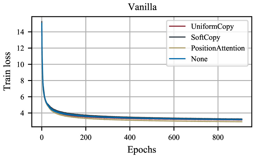
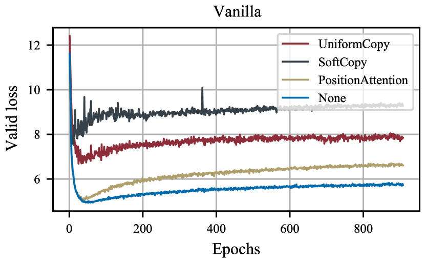
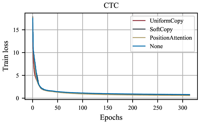
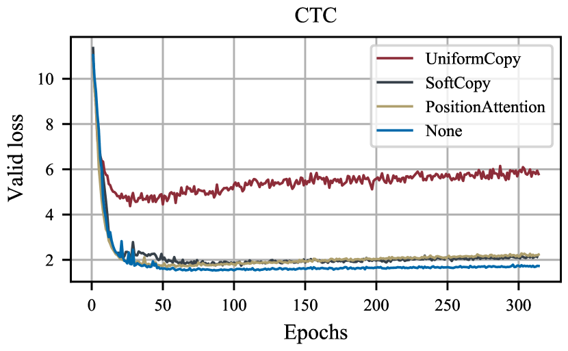
Figure 1: Influence of guided decoder input for VanillaNAT (top) and CTC (bottom) on the training (left) and validation (right) loss using the WMT’13 EN$\rightarrow$DE evaluation set.

Interestingly, for a setup without guided decoder input, especially the token embedding as well as the self-attention component in the first decoder layer supposedly contain only little information since only consecutive special tokens i.e. <unk>’s are passed. We investigate the performance contribution of these in Table 3 and observe that 1) the self-attention component in the first decoder layer only has minor impact and 2) solely relying on learned positional embeddings is sufficient for achieving comparable performance. However, we do keep both components in the main results for comparability reasons.

Models	WMT’13	WMT’14
	EN$\rightarrow$DE	EN$\rightarrow$DE
CTC	24.9	25.8
(Saharia et al., 2020)
+ no layer 0 self attention	25.0 ($\mathbf{\mathbin{\mathchoice{\hbox to9.99997pt{\hss$\displaystyle+$\hss}}{\hbox to9.99997pt{\hss$\textstyle+$\hss}}{\hbox to7.66663pt{\hss$\scriptstyle+$\hss}}{\hbox to6.11107pt{\hss$\scriptscriptstyle+$\hss}}}0.1}$)	25.5 ($\mathbf{\mathbin{\mathchoice{\hbox to9.99997pt{\hss$\displaystyle-$\hss}}{\hbox to9.99997pt{\hss$\textstyle-$\hss}}{\hbox to7.66663pt{\hss$\scriptstyle-$\hss}}{\hbox to6.11107pt{\hss$\scriptscriptstyle-$\hss}}}0.3}$)
+ no decoder embeddings	24.7 ($\mathbf{\mathbin{\mathchoice{\hbox to9.99997pt{\hss$\displaystyle-$\hss}}{\hbox to9.99997pt{\hss$\textstyle-$\hss}}{\hbox to7.66663pt{\hss$\scriptstyle-$\hss}}{\hbox to6.11107pt{\hss$\scriptscriptstyle-$\hss}}}0.2}$)	25.8 ($\mathbf{\mathbin{\mathchoice{\hbox to9.99997pt{\hss$\displaystyle-$\hss}}{\hbox to9.99997pt{\hss$\textstyle-$\hss}}{\hbox to7.66663pt{\hss$\scriptstyle-$\hss}}{\hbox to6.11107pt{\hss$\scriptscriptstyle-$\hss}}}0.2}$)
+ both	24.9 ($\mathbf{\mathbin{\mathchoice{\hbox to9.99997pt{\hss$\displaystyle+$\hss}}{\hbox to9.99997pt{\hss$\textstyle+$\hss}}{\hbox to7.66663pt{\hss$\scriptstyle+$\hss}}{\hbox to6.11107pt{\hss$\scriptscriptstyle+$\hss}}}0.0}$)	25.5 ($\mathbf{\mathbin{\mathchoice{\hbox to9.99997pt{\hss$\displaystyle-$\hss}}{\hbox to9.99997pt{\hss$\textstyle-$\hss}}{\hbox to7.66663pt{\hss$\scriptstyle-$\hss}}{\hbox to6.11107pt{\hss$\scriptscriptstyle-$\hss}}}0.3}$)
CTC + GLAT	25.8	26.0
(Qian et al., 2021)
+ no layer 0 self attention	25.8 ($\mathbf{\mathbin{\mathchoice{\hbox to9.99997pt{\hss$\displaystyle+$\hss}}{\hbox to9.99997pt{\hss$\textstyle+$\hss}}{\hbox to7.66663pt{\hss$\scriptstyle+$\hss}}{\hbox to6.11107pt{\hss$\scriptscriptstyle+$\hss}}}0.0}$)	25.9 ($\mathbf{\mathbin{\mathchoice{\hbox to9.99997pt{\hss$\displaystyle-$\hss}}{\hbox to9.99997pt{\hss$\textstyle-$\hss}}{\hbox to7.66663pt{\hss$\scriptstyle-$\hss}}{\hbox to6.11107pt{\hss$\scriptscriptstyle-$\hss}}}0.1}$)

Table 3: Overview of the translation quality implications when removing decoder components.

3.3.2 Influence of dropout

Dropout is one of the hyperparameters which either prior works did not mention or simply used the default values from previous studies. We performed a sweep for different architectures and language pairs, where we varied the dropout probability from $0$ to $0.5$, with increments of $0.1$ (see Figure A1). We observe that choosing an appropriate dropout rate is important for achieving high translation quality. In particular, for EN$\leftrightarrow$DE, $0.1$ achieves the best validation performance for all models, confirming the choice in prior works. For EN$\leftrightarrow$RO, we find that the value used in prior works, $0.3$, is optimal for non-CTC models, but, for CTC-based approaches, higher values seem to outperform.

3.3.3 Miscellaneous optimization choices

Many previous works use the Gaussian Error Linear Unit (GELU, Hendrycks and Gimpel, 2016) activation function, initialize the parameters with the procedure from BERT (Devlin et al., 2019), use length offset prediction, or a larger Adam (Kingma and Ba, 2015) $\epsilon$ value for optimization. In Section C.2 we summarize the effect of these choices and find that for Vanilla NAT models these variations regularly have a positive impact on translation quality but for CTC-based models the picture is less clear and rarely leads to consistent Bleu improvements. Based on these results, we deploy all choices besides $\epsilon$ tuning for non-CTC variants but omit them for CTC-based models.

3.4 Model comparison

Our results are consistent across the language pairs and metrics shown in Sections 3, D.3, and D.3, and align with former work (Gu and Kong, 2021). The most significant translation quality improvement can be achieved by switching from the traditional length prediction module to a CTC-based variant, confirming the strong dependence on accurate length predictions (Wang et al., 2021). This amounts to the largest accuracy increase that is achievable with current non-autoregressive methods but comes with a slight CPU latency increase due to the upsampling process. On top of this, GLAT consistently increases translation quality further by a significant margin. Deep Supervision can further increase the quality but, for the most part, not by a significant amount. Notably, though, it rarely hurts accuracy for our experiments across all three metrics and can sometimes even achieve a significant increase on top of CTC (RO$\rightarrow$EN on all three metrics and EN$\leftrightarrow$DE on Ter). See Appendix E for analysis on the predicted translations.

Comparing the strongest AT and NAT system in Table 4, we can see that despite Bleu parity on WMT’14 DE$\rightarrow$EN, the Comet scores (Rei et al., 2020) and our human evaluation results still indicate a quality gap between the two. Hence, metrics beyond Bleu are vital for rating NAT quality.

In terms of expected inference speed for non-autoregressive models, we believe that our latency numbers are more realistic than what is commonly reported in the literature. By considering additional speed-up techniques, improvements shrink to roughly $7.0\times$ on GPU and around $2.5\times$ on CPU.

Metric	WMT’14
	EN$\rightarrow$DE		DE$\rightarrow$EN
	$\Delta$	p-value	$\Delta$	p-value
Bleu $\uparrow$	$0.9$	$0.001$	$0.0$	$0.397$
chrF++ $\uparrow$	$0.3$	$0.009$	$-0.3$	$0.002$
Ter $\downarrow$	$-1.0$	$0.001$	$-1.0$	$0.001$
Comet $\uparrow$	$0.3$	$0.000$	$0.1$	$0.000$
Human Evaluation $\uparrow$	$7.5$	$0.000$	$1.1$	$0.000$

Table 4: Score deltas (AT score $-$ NAT score) of best autoregressive vs. non-autoregressive models on the WMT’14 EN$\leftrightarrow$DE test sets with p-values of the corresponding significance tests (paired bootstrap resampling for Bleu, chrF++, Ter, Comet; paired Student’s t-test for Human Acceptability Evaluation).

4 Conclusion

In this work, we provide multiple standardized sacreBLEU metrics for non-autoregressive machine translation models, accompanied by reproducible and modular fairseq code. We hope that our work solves comparison problems in the literature, provides more realistic speed-up expectations, and accelerates research in this area to achieve parity with autoregressive models in the future.

Limitations

While our work improves upon the state of translation quality and speed comparisons in the NAT literature, we acknowledge that there are many more low-level optimizations (e.g. porting the Python code to C++ and writing dedicated CUDA kernels) that could be made to improve the presented work. This would allow for an even more realistic inference speed comparison and enable direct comparability to e.g. Marian (Junczys-Dowmunt et al., 2018a) which is currently not given. There exists a concurrent work by Helcl et al. (2022) that tries to address some of these shortcomings by providing a CTC implementation in C++ and comparing the inference speed across different batching scenarios.

Apart from this limitation specific to our work, current non-autoregressive models still have a strong dependency on appropriate knowledge distillation from an autoregressive teacher that is able to effectively reduce data modes and limit the multimodality problem. While this already shows to be an important factor for achieving good translation quality on benchmarking datasets such as WMT, it is even more relevant for larger and/or multilingual datasets (Agrawal et al., 2021) that tend to be of higher complexity. Even though non-autoregressive models can lead to improved inference speed, this strong dependency still requires additional effort for tuning effective teacher architectures, conducting multiple training procedures, and generating simplified data through one or more distillation rounds. Until these problems are solved, it seems unrealistic that the average practitioner, who does not have access to a lot of compute, can effectively deploy these in production settings as general-purpose translation models. Apart from that, there is still more work needed in reducing the multimodality problem through more suitable architectures, optimization objectives, or a better data selection process.

Acknowledgements

We would like to thank Matthias Sperber for coordinating the publication process and Yi-Hsiu Liao for providing the Shortlist implementation. Further, we’d like to thank Sarthak Garg, Hendra Setiawan, Luke Carlson, Russ Webb, and Jesse Allardice for their helpful comments on the manuscript. Many thanks to Sachin Mehta and David Harrison for suggesting interesting ideas and the rest of Apple’s Machine Translation Team for their support.

Appendix A Related work

Many works have tried to accomplish the goal of autoregressive translation quality with a non-autoregressive model in recent years. The first paper to outline the vanilla non-autoregressive model for machine translation was Gu et al. (2018). After that, a few branches of work emerged that either focus on the multimodality problem (Ma et al., 2019; Ding et al., 2020; Qian et al., 2021; Ran et al., 2021; Bao et al., 2021; Song et al., 2021; Huang et al., 2022), on improving the knowledge transfer from autoregressive to non-autoregressive models (Li et al., 2019; Wei et al., 2019; Sun and Yang, 2020; Zhou et al., 2020; Guo et al., 2020; Hao et al., 2021; Xu et al., 2021), on applying different training objectives to train the non-autoregressive model (Libovický and Helcl, 2018; Ghazvininejad et al., 2020; Du et al., 2021; Shao et al., 2021), or on incorporating language models to boost accuracy (Su et al., 2021).

There is also a branch of work that focuses on semi-autoregressive models that try to find a balance between autoregressive and non-autoregressive models to leverage the benefits of both approaches (Stern et al., 2018; Lee et al., 2018; Gu et al., 2019; Ghazvininejad et al., 2019; Kasai et al., 2020; Chan et al., 2020). However, since they often mitigate the expected speed-up gains, we do not consider them in this work.

Appendix B Methods

In this section, we want to highlight some of the building blocks we used and explain their usage and configuration in our models.

B.1 Glancing Transformers

The Glancing Transformer (GLAT, Qian et al., 2021) tackles the multimodality problem by encouraging word interdependence through glancing sampling. In that, they adaptively select a number of ground truth tokens by comparing them to the model predictions $\hat{e}_{1}^{\hat{I}}$ and feeding the embeddings of the selected tokens to the decoder during training. Formally, the probability distribution can be described as

$$p_{\bm{\theta}}(e_{1}^{I}|f_{1}^{J})=\prod_{i=1}^{I}p_{\bm{\theta}}(e_{i}|\Phi(e_{1}^{I},\hat{e}_{1}^{\hat{I}}),f_{1}^{J}),$$ (3)

where $\Phi(e_{1}^{I},\hat{e}_{1}^{\hat{I}})$ represents the subset of tokens selected by the glancing sampling strategy. This sampling process can be split into two parts. First, determining the number of sampled tokens $S$ by comparing $e_{1}^{I}$ and $\hat{e}_{1}^{\hat{I}}$, here defined by the function $\Gamma(e_{1}^{I},\hat{e}_{1}^{\hat{I}})$. Secondly, selecting $S$ tokens from the ground truth that form the final output of the glancing sampling. Qian et al. (2021) deploy a random function for this purpose which we adopt and define here as the function $\Omega(e_{1}^{I},S)$. Combining all these, the sampling strategy can be formulated as

$$\Phi(e_{1}^{I},\hat{e}_{1}^{\hat{I}})=\Omega(e_{1}^{I},\Gamma(e_{1}^{I},\hat{e}_{1}^{\hat{I}})),$$ (4)

with the number of sampled tokens $S$ being determined by $\Gamma(e_{1}^{I},\hat{e}_{1}^{\hat{I}})=\lambda\cdot d(e_{1}^{I},\hat{e}_{1}^{\hat{I}})$ where $d(e_{1}^{I},\hat{e}_{1}^{\hat{I}})$ is a distance measure between the ground truth $e_{1}^{I}$ and the predicted tokens $\hat{e}_{1}^{\hat{I}}$ while $\lambda$ is a hyperparameter. For this distance measure, there are many choices that can be deployed in theory such as the Levenshtein distance (Levenshtein, 1966) or, with slight adaptions, one of the Bregman divergences (Banerjee et al., 2005). For their experiments, Qian et al. (2021) choose the Hamming distance (Hamming, 1950) defined as $d(e_{1}^{I},\hat{e}_{1}^{\hat{I}})=\sum_{i=1}^{I}e_{i}\neq\hat{e}_{i}$ which has the useful property that it takes into account the current prediction quality of the model, causing the number of sampled tokens $S$ to be high initially and decrease over time. In their implementation, they additionally deploy a linearly decreasing schedule with a lower bound i.e. $\lambda=\lambda_{s}-\lambda_{m}\cdot\frac{u}{U}$ where $u$ is the current and $U$ is the maximum number of update steps with $\lambda_{s}=0.5$ and $\lambda_{m}=0.2$ to further control the number of sampled tokens. We adopt their configuration.

B.2 Connectionist Temporal Classification

Traditional sequence-to-sequence models output target tokens autoregressively until an end-of-sentence token is encountered and are trained using the standard cross-entropy loss. In a non-autoregressive setting, though, the number of tokens in the output is not known a priori. One solution is to train a length prediction module to determine the number of output tokens, but this approach still has drawbacks, as it doesn’t properly address token repetition and the predicted length can easily be either too short or too long. The quality of the length prediction module is influenced by properties of the respective language pairs such as alignment patterns, word orders or intrinsic length ratios (Wang et al., 2021). These fluctuations in accuracy are especially influential on the final translation quality (Wang et al., 2021).

The Connectionist Temporal Classification (CTC, Graves et al., 2006; Libovický and Helcl, 2018) approach tries to improve this property by setting a large enough output length $\tilde{J}$ and giving the model the option to flexibly adjust the target offsets using an additional <blank> token. Specifically, by marginalizing all possible alignments using dynamic programming, for all aligned sequences $a_{1}^{\tilde{J}}$ that can be reduced to the target $e_{1}^{I}$, the conditional probability corresponds to

$$\begin{split}p_{\bm{\theta}}(e_{1}^{I}|f_{1}^{J})&=\sum_{a_{1}^{\tilde{J}}\in\mathcal{A}(e_{1}^{I})}p_{\bm{\theta}}(a_{1}^{\tilde{J}}|f_{1}^{J})\\ &=\sum_{a_{1}^{\tilde{J}}\in\mathcal{A}(e_{1}^{I})}\prod_{j=1}^{\tilde{J}}p_{\bm{\theta}}(a_{j}|f_{1}^{J})\end{split}$$ (5)

where $\mathcal{A}$ is a one-to-many map that produces all possible alignments $a_{1}^{\tilde{J}}$ and $\mathcal{A}^{-1}$ is a many-to-one map that collapses an alignment to recover the target sequence by first removing repeated and then <blank> tokens e.g.

$$\mathcal{A}^{-1}(\underbrace{\bigstrut[b]a-abb}_{a_{1}^{5}})=\mathcal{A}^{-1}(\underbrace{\bigstrut[b]aa-ab}_{a_{1}^{5}})=\underbrace{\bigstrut[b]aab}_{e_{1}^{3}}$$ (6)

with $-$ representing the <blank> token for brevity. This approach requires setting an alignment length $\tilde{J}$ that is determined by a scaling factor $s$ commonly chosen to be $2$ – $3$ times the source length $J$, i.e. $\tilde{J}=J\cdot s$. In the example of Equation 6, the alignment length is $\tilde{J}=5$.

Combining with GLAT

To effectively combine CTC with GLAT, an alignment for the target tokens is required to enable the glancing sampling correspondence with the decoder input tokens. For that, Gu and Kong (2021) suggest using the Viterbi aligned tokens

$$\hat{a}_{1}^{\tilde{J}}(f_{1}^{J})=\operatorname*{arg\,max}_{a_{1}^{\tilde{J}}\in\mathcal{A}(e_{1}^{I})}\ p_{\bm{\theta}}(a_{1}^{\tilde{J}}|f_{1}^{J})$$ (7)

which we adopt in our implementation and obtain leveraging the best_alignment method from the Imputer (Chan et al., 2020). Similar to previous works, we use greedy decoding instead of beam search for all our experiments to keep a strict non-autoregressive property.

B.3 Deep Supervision

The Deeply Supervised Layer-wise Prediction-aware Transformer (DSLP, Huang et al., 2022) introduces three strategies to address the multimodality problem. Namely, Deep Supervision, Layer-Wise Prediction-Awareness, and Mixed Training. In a nutshell, Deep Supervision refers to predicting the output tokens at every decoder layer, computing the layer-wise losses, and aggregating them to form the overall loss used for optimizing the model. Formally, we can maximize the log-likelihood

$$\mathcal{L}=\frac{1}{L_{D}}\sum_{l=1}^{L_{D}}\sum_{i=1}^{I}\log p_{\bm{\theta}}^{(l)}(e_{i}^{(l)}|\bm{h}^{(l)}_{i}),$$ (8)

where $\bm{h}^{(l)}_{i}$ is the hidden state of decoder layer $l$ corresponding to position $i$ and $L_{D}$ is the overall number of decoder layers. Intuitively, this approach loses its value when moving to a deep encoder and shallow decoder (Kasai et al., 2021) with $L_{D}=1$.

While Deep Supervision keeps the model parameter count constant and only increases the used memory, the other two proposed techniques increase the number of trained parameters. For this work, we only adopt the Deep Supervision part due to the aforementioned drawback.

Appendix C Ablations

C.1 Influence of dropout

Figure A1 shows the Bleu score plotted against the dropout rate for all translation directions and multiple architectures. In general, our results agree with the choices of prior work with $0.1$ performing best for EN$\leftrightarrow$DE, and $0.3$ for EN$\leftrightarrow$RO. For the CTC-based methods, higher dropouts seem to give slightly better results.

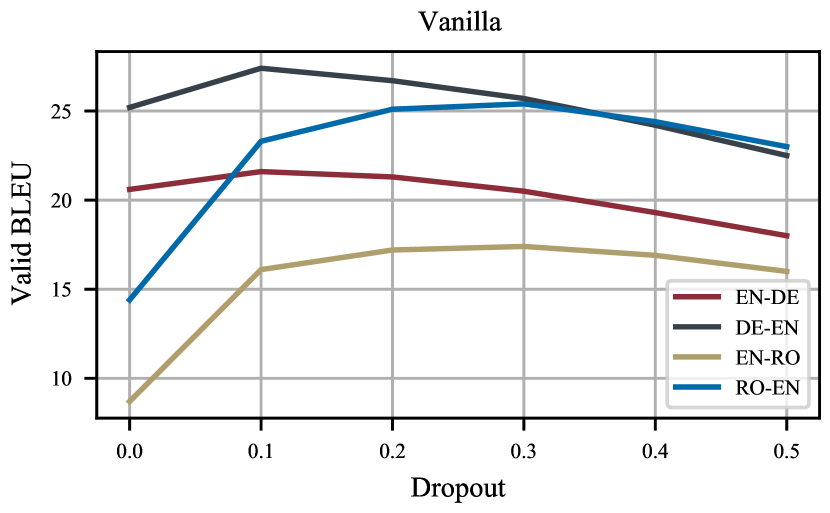
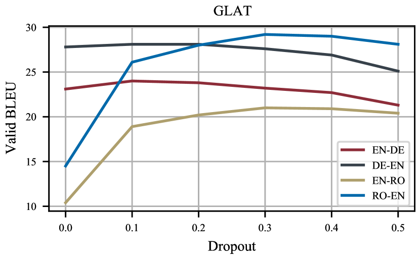
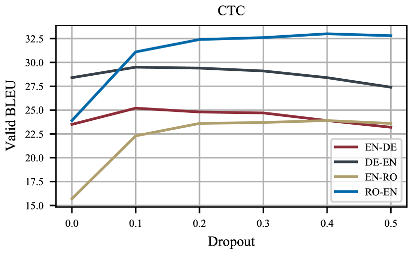
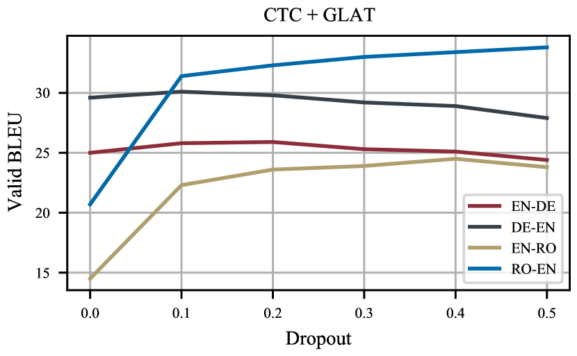
Figure A1: Influence of dropout for different models and language pairs on the respective validation set.

C.2 Optimization choices

We conduct experiments to assess the value of more optimization choices in Table A1. From these, it seems that most of them seem to have a positive impact when being deployed for non-CTC variants while they don’t seem to benefit CTC-based variants.

Models	WMT’13	WMT’14
	EN$\rightarrow$DE	EN$\rightarrow$DE
Vanilla NAT	21.1	20.0
(Gu et al., 2018)
+ GELU	21.4 ($\mathbf{\mathbin{\mathchoice{\hbox to9.99997pt{\hss$\displaystyle+$\hss}}{\hbox to9.99997pt{\hss$\textstyle+$\hss}}{\hbox to7.66663pt{\hss$\scriptstyle+$\hss}}{\hbox to6.11107pt{\hss$\scriptscriptstyle+$\hss}}}0.3}$)	20.0 ($\mathbf{\mathbin{\mathchoice{\hbox to9.99997pt{\hss$\displaystyle+$\hss}}{\hbox to9.99997pt{\hss$\textstyle+$\hss}}{\hbox to7.66663pt{\hss$\scriptstyle+$\hss}}{\hbox to6.11107pt{\hss$\scriptscriptstyle+$\hss}}}0.0}$)
+ BERT init	21.3 ($\mathbf{\mathbin{\mathchoice{\hbox to9.99997pt{\hss$\displaystyle+$\hss}}{\hbox to9.99997pt{\hss$\textstyle+$\hss}}{\hbox to7.66663pt{\hss$\scriptstyle+$\hss}}{\hbox to6.11107pt{\hss$\scriptscriptstyle+$\hss}}}0.2}$)	20.1 ($\mathbf{\mathbin{\mathchoice{\hbox to9.99997pt{\hss$\displaystyle+$\hss}}{\hbox to9.99997pt{\hss$\textstyle+$\hss}}{\hbox to7.66663pt{\hss$\scriptstyle+$\hss}}{\hbox to6.11107pt{\hss$\scriptscriptstyle+$\hss}}}0.1}$)
+ Predict length offset	21.4 ($\mathbf{\mathbin{\mathchoice{\hbox to9.99997pt{\hss$\displaystyle+$\hss}}{\hbox to9.99997pt{\hss$\textstyle+$\hss}}{\hbox to7.66663pt{\hss$\scriptstyle+$\hss}}{\hbox to6.11107pt{\hss$\scriptscriptstyle+$\hss}}}0.3}$)	20.0 ($\mathbf{\mathbin{\mathchoice{\hbox to9.99997pt{\hss$\displaystyle+$\hss}}{\hbox to9.99997pt{\hss$\textstyle+$\hss}}{\hbox to7.66663pt{\hss$\scriptstyle+$\hss}}{\hbox to6.11107pt{\hss$\scriptscriptstyle+$\hss}}}0.0}$)
+ Adam $\epsilon=1e-6$	21.2 ($\mathbf{\mathbin{\mathchoice{\hbox to9.99997pt{\hss$\displaystyle+$\hss}}{\hbox to9.99997pt{\hss$\textstyle+$\hss}}{\hbox to7.66663pt{\hss$\scriptstyle+$\hss}}{\hbox to6.11107pt{\hss$\scriptscriptstyle+$\hss}}}0.1}$)	20.1 ($\mathbf{\mathbin{\mathchoice{\hbox to9.99997pt{\hss$\displaystyle+$\hss}}{\hbox to9.99997pt{\hss$\textstyle+$\hss}}{\hbox to7.66663pt{\hss$\scriptstyle+$\hss}}{\hbox to6.11107pt{\hss$\scriptscriptstyle+$\hss}}}0.1}$)
CTC	25.0	25.6
(Saharia et al., 2020)
+ GELU	25.0 ($\mathbf{\mathbin{\mathchoice{\hbox to9.99997pt{\hss$\displaystyle+$\hss}}{\hbox to9.99997pt{\hss$\textstyle+$\hss}}{\hbox to7.66663pt{\hss$\scriptstyle+$\hss}}{\hbox to6.11107pt{\hss$\scriptscriptstyle+$\hss}}}0.0}$)	25.5 ($\mathbf{\mathbin{\mathchoice{\hbox to9.99997pt{\hss$\displaystyle-$\hss}}{\hbox to9.99997pt{\hss$\textstyle-$\hss}}{\hbox to7.66663pt{\hss$\scriptstyle-$\hss}}{\hbox to6.11107pt{\hss$\scriptscriptstyle-$\hss}}}0.1}$)
+ BERT init	24.8 ($\mathbf{\mathbin{\mathchoice{\hbox to9.99997pt{\hss$\displaystyle-$\hss}}{\hbox to9.99997pt{\hss$\textstyle-$\hss}}{\hbox to7.66663pt{\hss$\scriptstyle-$\hss}}{\hbox to6.11107pt{\hss$\scriptscriptstyle-$\hss}}}0.2}$)	25.6 ($\mathbf{\mathbin{\mathchoice{\hbox to9.99997pt{\hss$\displaystyle+$\hss}}{\hbox to9.99997pt{\hss$\textstyle+$\hss}}{\hbox to7.66663pt{\hss$\scriptstyle+$\hss}}{\hbox to6.11107pt{\hss$\scriptscriptstyle+$\hss}}}0.0}$)
+ Adam $\epsilon=1e-6$	25.2 ($\mathbf{\mathbin{\mathchoice{\hbox to9.99997pt{\hss$\displaystyle+$\hss}}{\hbox to9.99997pt{\hss$\textstyle+$\hss}}{\hbox to7.66663pt{\hss$\scriptstyle+$\hss}}{\hbox to6.11107pt{\hss$\scriptscriptstyle+$\hss}}}0.2}$)	25.7 ($\mathbf{\mathbin{\mathchoice{\hbox to9.99997pt{\hss$\displaystyle+$\hss}}{\hbox to9.99997pt{\hss$\textstyle+$\hss}}{\hbox to7.66663pt{\hss$\scriptstyle+$\hss}}{\hbox to6.11107pt{\hss$\scriptscriptstyle+$\hss}}}0.1}$)

Table A1: Overview of the quality implications when adding different optimization techniques. Distilled training data and hyperparameters stay consistent and results are reported for the evaluation sets of WMT’13 and WMT’14 for EN$\rightarrow$DE.

Table A1 suggests that choosing a slightly higher Adam $\epsilon$ might have a positive effect for training non-autoregressive models. To this end, we ran a grid search in the range $[1\mathrm{e}{-9},1\mathrm{e}{-1}]$ with a delta factor between samples of $\Delta=10^{-1}$ for CTC + GLAT, one of our top-performing models, to verify the observed gains. The results of this experiment can be seen in Table A2.

Models	WMT’13	WMT’14
	EN$\rightarrow$DE	EN$\rightarrow$DE
CTC + GLAT	25.8	25.9
(Qian et al., 2021)
+ Adam $\epsilon=1e-9$	25.9 ($\mathbf{\mathbin{\mathchoice{\hbox to9.99997pt{\hss$\displaystyle+$\hss}}{\hbox to9.99997pt{\hss$\textstyle+$\hss}}{\hbox to7.66663pt{\hss$\scriptstyle+$\hss}}{\hbox to6.11107pt{\hss$\scriptscriptstyle+$\hss}}}0.1}$)	25.9 ($\mathbf{\mathbin{\mathchoice{\hbox to9.99997pt{\hss$\displaystyle+$\hss}}{\hbox to9.99997pt{\hss$\textstyle+$\hss}}{\hbox to7.66663pt{\hss$\scriptstyle+$\hss}}{\hbox to6.11107pt{\hss$\scriptscriptstyle+$\hss}}}0.0}$)
+ Adam $\epsilon=1e-7$	25.8 ($\mathbf{\mathbin{\mathchoice{\hbox to9.99997pt{\hss$\displaystyle+$\hss}}{\hbox to9.99997pt{\hss$\textstyle+$\hss}}{\hbox to7.66663pt{\hss$\scriptstyle+$\hss}}{\hbox to6.11107pt{\hss$\scriptscriptstyle+$\hss}}}0.0}$)	26.0 ($\mathbf{\mathbin{\mathchoice{\hbox to9.99997pt{\hss$\displaystyle+$\hss}}{\hbox to9.99997pt{\hss$\textstyle+$\hss}}{\hbox to7.66663pt{\hss$\scriptstyle+$\hss}}{\hbox to6.11107pt{\hss$\scriptscriptstyle+$\hss}}}0.1}$)
+ Adam $\epsilon=1e-6$	25.7 ($\mathbf{\mathbin{\mathchoice{\hbox to9.99997pt{\hss$\displaystyle-$\hss}}{\hbox to9.99997pt{\hss$\textstyle-$\hss}}{\hbox to7.66663pt{\hss$\scriptstyle-$\hss}}{\hbox to6.11107pt{\hss$\scriptscriptstyle-$\hss}}}0.1}$)	25.9 ($\mathbf{\mathbin{\mathchoice{\hbox to9.99997pt{\hss$\displaystyle+$\hss}}{\hbox to9.99997pt{\hss$\textstyle+$\hss}}{\hbox to7.66663pt{\hss$\scriptstyle+$\hss}}{\hbox to6.11107pt{\hss$\scriptscriptstyle+$\hss}}}0.0}$)
+ Adam $\epsilon=1e-5$	25.7 ($\mathbf{\mathbin{\mathchoice{\hbox to9.99997pt{\hss$\displaystyle-$\hss}}{\hbox to9.99997pt{\hss$\textstyle-$\hss}}{\hbox to7.66663pt{\hss$\scriptstyle-$\hss}}{\hbox to6.11107pt{\hss$\scriptscriptstyle-$\hss}}}0.1}$)	25.6 ($\mathbf{\mathbin{\mathchoice{\hbox to9.99997pt{\hss$\displaystyle-$\hss}}{\hbox to9.99997pt{\hss$\textstyle-$\hss}}{\hbox to7.66663pt{\hss$\scriptstyle-$\hss}}{\hbox to6.11107pt{\hss$\scriptscriptstyle-$\hss}}}0.3}$)
+ Adam $\epsilon=1e-4$	25.3 ($\mathbf{\mathbin{\mathchoice{\hbox to9.99997pt{\hss$\displaystyle-$\hss}}{\hbox to9.99997pt{\hss$\textstyle-$\hss}}{\hbox to7.66663pt{\hss$\scriptstyle-$\hss}}{\hbox to6.11107pt{\hss$\scriptscriptstyle-$\hss}}}0.5}$)	25.1 ($\mathbf{\mathbin{\mathchoice{\hbox to9.99997pt{\hss$\displaystyle-$\hss}}{\hbox to9.99997pt{\hss$\textstyle-$\hss}}{\hbox to7.66663pt{\hss$\scriptstyle-$\hss}}{\hbox to6.11107pt{\hss$\scriptscriptstyle-$\hss}}}0.8}$)
+ Adam $\epsilon=1e-3$	22.0 ($\mathbf{\mathbin{\mathchoice{\hbox to9.99997pt{\hss$\displaystyle-$\hss}}{\hbox to9.99997pt{\hss$\textstyle-$\hss}}{\hbox to7.66663pt{\hss$\scriptstyle-$\hss}}{\hbox to6.11107pt{\hss$\scriptscriptstyle-$\hss}}}3.8}$)	21.2 ($\mathbf{\mathbin{\mathchoice{\hbox to9.99997pt{\hss$\displaystyle-$\hss}}{\hbox to9.99997pt{\hss$\textstyle-$\hss}}{\hbox to7.66663pt{\hss$\scriptstyle-$\hss}}{\hbox to6.11107pt{\hss$\scriptscriptstyle-$\hss}}}4.7}$)
+ Adam $\epsilon=1e-2$	diverges	diverges
+ Adam $\epsilon=1e-1$	diverges	diverges

Table A2: Overview of the quality implications when changing the Adam $\epsilon$ for CTC + GLAT. The baseline run uses the default of $\epsilon=1\mathrm{e}{-8}$.

From our results we conclude that the observed gains are neither consistent nor statistically significant as they don’t transfer to the CTC + GLAT model without further tuning of the remaining hyperparamaters such as the learning rate $\eta$ or the Adam momentum terms $\beta_{1}$ and $\beta_{2}$. To simplify hyperparameter transfer to evolving production datasets and randomness in the training procedure without any additional tuning, we keep the default of $\epsilon=1e-8$ (similar to Schmidt et al., 2021) for our models that use a combination of methods such as CTC + GLAT or CTC + DS and advise the community to avoid this type of tuning for comparability. While it may seem appealing at first, it can distort expected translation quality gains for novel methods as commonly this sort of tuning is only conducted for the introduced method at hand but not, or only marginally, for baselines or competing algorithms. Any gain that is achieved through such practices should not be accredited to the introduced method as other algorithms are most likely able to achieve similar gains through an equal amount of hyperparameter tuning.

Appendix D Result details

D.1 Dataset

We preprocessed the datasets using Moses scripts (Koehn et al., 2007) to tokenize all datasets, clean the data (clean-corpus-n.pl), and normalize punctuation (normalize-punctuation.perl). No True-Casing is used. For RO$\rightarrow$EN we normalize Romanian and remove diacritics using WMT’16 provided scripts. EN$\rightarrow$RO keeps diacritics for producing accurate translations which explains the gap between our numbers and those claimed in previous works (Gu and Kong, 2021; Qian et al., 2021; Gu et al., 2018), who besides computing Bleu on tokenized text, compared on diacritic-free text.

For ablations, which are only conducted on WMT’14 EN$\rightarrow$DE distilled training data, we additionally report accuracy on the WMT’13 EN$\rightarrow$DE evaluation set, serving as validation performance. We use a shared source and target vocabulary for all language directions, obtained using BPE with $40$k merge operations where the distillation process dropped around $400-800$ tokens depending on the respective target language.

D.2 Signatures: sacreBLEU

We use sacreBLEU version $2.0.0$. The evaluation signatures for Bleu (Papineni et al., 2002) are nrefs:1 | case:mixed | eff:no | tok:13a | smooth:exp. Additionally we also report chrF++ (Popović, 2017) with nrefs:1 | case:mixed | eff:yes | nc:6 | nw:2 | space:no and Ter (Snover et al., 2006) with nrefs:1 | case:mixed | tok:tercom | norm:no | punct:yes | asian:no for the main results.

D.3 Paired boostrap resampling

For the boostrap resampling used to identify non-significant results in the main tables, we always use the root level of the sub-blocks (separated by dashed lines) as base system within that specific sub-block. For models that deploy multiple additional methods, e.g. CTC + GLAT + DS, we always use the previous row as the base system, e.g. CTC + GLAT in this case. This procedure is especially relevant for the significance tests on the autoregressive baselines that use knowledge distillation, average attention, and shortlists and helps to show the significance of the individual methods on the translation quality. While we want significant results for the NAT category, it is beneficial to have non-significant results for the methods that are deployed to speed-up CPU inference (i.e. average attention and shortlists) as this shows that the respective model is not statistically different while offering faster CPU inference. Finally, for the root levels of each sub-block we use the first sub-block of each category as the base system i.e. both CTC and CTC (11-2) are compared to Vanilla-NAT while Transformer base (11-2) is compared to Transformer base. The null hypothesis is always that the reference system and the baseline translations are essentially generated by the same underlying process. If they are marked with ^†, the null hypothesis could not be rejected.

Additional Metrics

Both Sections D.3 and D.3, which report chrF++ and Ter, support our conclusions drawn in Section 3.4 of the main paper, statistical significance sometimes deviates marginally.

Models

$|\bm{\theta}|$

WMT’13

WMT’14

WMT’16

Speed

Latency GPU

Speed

Latency CPU

EN$\rightarrow$DE

EN$\rightarrow$DE

DE$\rightarrow$EN

EN$\rightarrow$RO

RO$\rightarrow$EN

(GPU)

($\mathrm{ms}$ / sentence)

(CPU)

($\mathrm{ms}$ / sentence)

Autoregressive

Transformer base

66M

$51.7$

$54.1$

$55.4$

$50.4$

$57.0$

0.5$\times$

$165.8$${}\pm{}$

$1.3$

0.3$\times$

$657.2$${}\pm{}$

$11.4$

+ Beam $5$ (teacher)

66M

$52.3$

$54.8$

$56.3$

$50.9$

$57.5$

0.4$\times$

$212.8$${}\pm{}$

$8.9$

0.1$\times$

$1272.4$${}\pm{}$

$38.5$

+ KD

66M

$52.2$

$54.8$

$55.6$

$50.7$

$57.1^{†}$

0.5$\times$

$173.4$${}\pm{}$

$1.0$

0.3$\times$

$646.3$${}\pm{}$

$8.9$

1-13 Transformer base (11-2)

63M $\downarrow$

$51.6^{†}$

$54.1^{†}$

$55.0$

$50.5^{†}$

$57.0^{†}$

0.9$\times$

$89.1$${}\pm{}$

$3.2$

0.4$\times$

$424.2$${}\pm{}$

$15.0$

+ KD

63M $\downarrow$

$52.2$

$54.9$

$56.0$

$50.6^{†}$

$57.1^{†}$

0.9$\times$

$88.1$${}\pm{}$

$1.5$

0.5$\times$

$408.0$${}\pm{}$

$3.2$

+ KD + AA

62M $\downarrow$

$52.2^{†}$

$54.8^{†}$

$55.7$

$50.7^{†}$

$57.0^{†}$

1.0$\times$

$79.4$${}\pm{}$

$2.2$

0.5$\times$

$396.9$${}\pm{}$

$5.4$

+ KD + AA + SL

62M $\downarrow$

$52.2^{†}$

$54.8^{†}$

$55.7$

$50.7^{†}$

$57.0$

1.0$\times$

$82.7$${}\pm{}$

$7.5$

1.0$\times$

$188.3$${}\pm{}$

$2.2$

Non-Autoregressive

Vanilla-NAT

66M

$48.5$

$50.2$

$52.5$

$46.6$

$52.8$

6.1$\times$

$13.1$${}\pm{}$

$0.3$

2.1$\times$

$90.1$${}\pm{}$

$0.4$

+ GLAT

66M

$50.5$

$52.7$

$54.4$

$48.4$

$54.5$

6.2$\times$

$12.8$${}\pm{}$

$0.4$

2.1$\times$

$90.4$${}\pm{}$

$0.6$

1-13 CTC

66M

$51.5$

$53.8$

$55.2$

$50.3$

$57.1$

6.4$\times$

$12.4$${}\pm{}$

$0.4$

1.5$\times$

$122.9$${}\pm{}$

$1.7$

+ DS

66M

$51.5^{†}$

$53.9^{†}$

$55.3^{†}$

$50.3^{†}$

$57.3$

6.3$\times$

$12.7$${}\pm{}$

$0.6$

1.6$\times$

$121.4$${}\pm{}$

$0.5$

+ GLAT

66M

$52.0$

$54.4$

$55.7$

$50.6$

$57.3$

6.3$\times$

$12.7$${}\pm{}$

$0.3$

1.6$\times$

$121.2$${}\pm{}$

$1.2$

+ GLAT + DS

66M

$52.1$

$54.6$

$55.9$

$50.7^{†}$

$57.3^{†}$

6.2$\times$

$12.8$${}\pm{}$

$0.3$

1.5$\times$

$121.8$${}\pm{}$

$0.4$

1-13 CTC (11-2)

63M $\downarrow$

$51.6$

$54.0$

$55.4$

$50.6$

$57.4$

6.9$\times$

$11.5$${}\pm{}$

$0.2$

1.6$\times$

$114.6$${}\pm{}$

$1.3$

+ GLAT

63M $\downarrow$

$52.0$

$54.5$

$56.0$

$51.0$

$57.6$

6.8$\times$

$11.7$${}\pm{}$

$0.4$

1.6$\times$

$114.6$${}\pm{}$

$1.2$

+ GLAT + SL

63M $\downarrow$

$52.0^{†}$

$54.5^{†}$

$56.0$

$51.0^{†}$

$57.6^{†}$

6.7$\times$

$11.9$${}\pm{}$

$0.2$

2.6$\times$

$72.5$${}\pm{}$

$0.8$

Table A3: Main results using chrF++ on four different translation directions. Latencies are measured on the WMT’14 EN$\rightarrow$DE test set as the average processing time per sentence using batch size $1$. All AT models require $I$ decoding iterations at inference time while the NAT models only require $1$. WMT’13 EN$\rightarrow$DE serves as validation performance. No re-scoring is used for all results. Statistically non-significant results using paired bootstrap resampling are marked with ^† for $p\geq 0.05$, see Section D.3 for more details. EN$\rightarrow$RO keeps diacritics and $\downarrow$ indicates less number of parameters than the baseline.

Models

$|\bm{\theta}|$

WMT’13

WMT’14

WMT’16

Speed

Latency GPU

Speed

Latency CPU

EN$\rightarrow$DE

EN$\rightarrow$DE

DE$\rightarrow$EN

EN$\rightarrow$RO

RO$\rightarrow$EN

(GPU)

($\mathrm{ms}$ / sentence)

(CPU)

($\mathrm{ms}$ / sentence)

Autoregressive

Transformer base

66M

$64.1$

$63.0$

$56.9$

$64.4$

$55.6$

0.5$\times$

$165.8$${}\pm{}$

$1.3$

0.3$\times$

$657.2$${}\pm{}$

$11.4$

+ Beam $5$ (teacher)

66M

$63.7$

$62.4$

$56.0$

$63.8$

$55.1$

0.4$\times$

$212.8$${}\pm{}$

$8.9$

0.1$\times$

$1272.4$${}\pm{}$

$38.5$

+ KD

66M

$64.0^{†}$

$62.9^{†}$

$56.3$

$64.0$

$55.5^{†}$

0.5$\times$

$173.4$${}\pm{}$

$1.0$

0.3$\times$

$646.3$${}\pm{}$

$8.9$

1-13 Transformer base (11-2)

63M $\downarrow$

$63.8^{†}$

$63.1^{†}$

$57.0^{†}$

$63.9$

$55.4^{†}$

0.9$\times$

$89.1$${}\pm{}$

$3.2$

0.4$\times$

$424.2$${}\pm{}$

$15.0$

+ KD

63M $\downarrow$

$63.7^{†}$

$62.4$

$55.6$

$63.7^{†}$

$55.3^{†}$

0.9$\times$

$88.1$${}\pm{}$

$1.5$

0.5$\times$

$408.0$${}\pm{}$

$3.2$

+ KD + AA

62M $\downarrow$

$63.8^{†}$

$62.4^{†}$

$55.4^{†}$

$63.6^{†}$

$55.7^{†}$

1.0$\times$

$79.4$${}\pm{}$

$2.2$

0.5$\times$

$396.9$${}\pm{}$

$5.4$

+ KD + AA + SL

62M $\downarrow$

$63.8^{†}$

$62.4^{†}$

$55.4$

$63.6^{†}$

$55.7$

1.0$\times$

$82.7$${}\pm{}$

$7.5$

1.0$\times$

$188.3$${}\pm{}$

$2.2$

Non-Autoregressive

Vanilla-NAT

66M

$67.9$

$68.1$

$60.1$

$68.0$

$59.4$

6.1$\times$

$13.1$${}\pm{}$

$0.3$

2.1$\times$

$90.1$${}\pm{}$

$0.4$

+ GLAT

66M

$65.5$

$65.1$

$58.0$

$66.2$

$57.8$

6.2$\times$

$12.8$${}\pm{}$

$0.4$

2.1$\times$

$90.4$${}\pm{}$

$0.6$

1-13 CTC

66M

$64.5$

$63.8$

$56.6$

$64.5$

$55.6$

6.4$\times$

$12.4$${}\pm{}$

$0.4$

1.5$\times$

$122.9$${}\pm{}$

$1.7$

+ DS

66M

$64.2$

$63.4$

$56.1$

$64.5^{†}$

$55.3$

6.3$\times$

$12.7$${}\pm{}$

$0.6$

1.6$\times$

$121.4$${}\pm{}$

$0.5$

+ GLAT

66M

$64.1$

$63.5^{†}$

$56.0$

$64.0$

$55.1$

6.3$\times$

$12.7$${}\pm{}$

$0.3$

1.6$\times$

$121.2$${}\pm{}$

$1.2$

+ GLAT + DS

66M

$64.1^{†}$

$63.3^{†}$

$55.9^{†}$

$64.2^{†}$

$55.4^{†}$

6.2$\times$

$12.8$${}\pm{}$

$0.3$

1.5$\times$

$121.8$${}\pm{}$

$0.4$

1-13 CTC (11-2)

63M $\downarrow$

$64.0$

$63.5$

$56.3$

$64.1$

$54.9$

6.9$\times$

$11.5$${}\pm{}$

$0.2$

1.6$\times$

$114.6$${}\pm{}$

$1.3$

+ GLAT

63M $\downarrow$

$64.4$

$63.4^{†}$

$56.4^{†}$

$63.7$

$55.1^{†}$

6.8$\times$

$11.7$${}\pm{}$

$0.4$

1.6$\times$

$114.6$${}\pm{}$

$1.2$

+ GLAT + SL

63M $\downarrow$

$64.4^{†}$

$63.4^{†}$

$56.4^{†}$

$63.7^{†}$

$55.1^{†}$

6.7$\times$

$11.9$${}\pm{}$

$0.2$

2.6$\times$

$72.5$${}\pm{}$

$0.8$

Table A4: Main results using Ter on four different translation directions. Latencies are measured on the WMT’14 EN$\rightarrow$DE test set as the average processing time per sentence using batch size $1$. All AT models require $I$ decoding iterations at inference time while the NAT models only require $1$. WMT’13 EN$\rightarrow$DE serves as validation performance. No re-scoring is used for all results. Statistically non-significant results using paired bootstrap resampling are marked with ^† for $p\geq 0.05$, see Section D.3 for more details. EN$\rightarrow$RO keeps diacritics and $\downarrow$ indicates less number of parameters than the baseline.

Appendix E Analysis

Hypotheses characteristics

Comparing one of the best performing NAT models, CTC + GLAT (11-2) to its autoregressive counterpart Transformer base (11-2), we try to understand the nature of occurring errors and their similarity. For that, we compare the Levenshtein distance between each models’ hypotheses and the reference as well as their hypotheses with each other in Figure A2 on the WMT’14 DE$\rightarrow$EN test set. Both AT and NAT follow a similar distribution of distance when compared to the reference. However, when comparing their hypothesis to each other, only $351/3003$ hypotheses match exactly and often we can observe Levenshtein distances between $0-50$. If we compare their sentence embeddings using BERT from sentence-transformers (Reimers and Gurevych, 2019) in Figure A3, we observe a similar trend when comparing them to the reference, although the autoregressive model is able to achieve slightly higher cosine similarity. Looking at samples with low cosine similarity between AT and NAT, we observe NAT problems that have been pointed out by prior work including repeated tokens and non-coherent sentences.

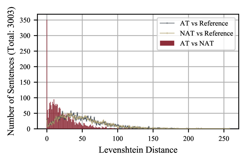
Figure A2: Levenshtein Distance between the hypotheses generated from the autoregressive Transformer base (11-2) + KD and CTC + GLAT (11-2) on the WMT’14 DE$\rightarrow$EN test set. Here, $351$ hypotheses match exactly. Individual distances of the hypotheses against the ground truth are plotted for reference.

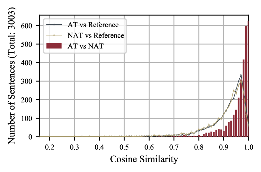
Figure A3: Cosine similarity for BERT hypothesis embeddings (mean final hidden state) generated from the autoregressive Transformer base (11-2) + KD and CTC + GLAT (11-2) on the WMT’14 DE$\rightarrow$EN test set.

Looking at the effect of sentence length on Bleu in Figure A4, we observe that for sequence lengths $<40$ the autoregressive models outperform the non-autoregressive models while for sequence lengths $>40$ we can see CTC + GLAT outperforming. We attribute this to the significantly smaller sample size for longer sentences.

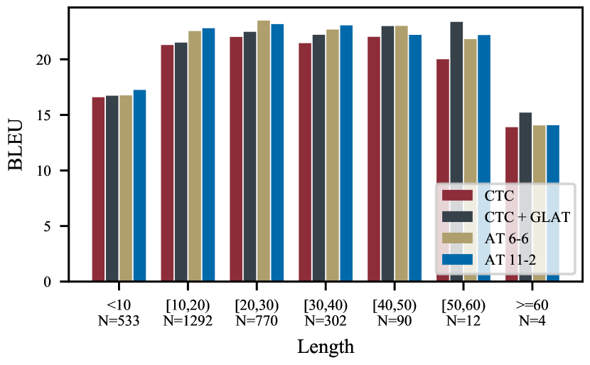
Figure A4: Effect of sentence length on Bleu for multiple architectures on WMT’14 EN$\rightarrow$DE test set. The height of each bucket reflects the corpus-level Bleu for that bucket, computed using compare-mt (Neubig et al., 2019). $N$ indicates the number of sentences in each bucket.

Human Evaluation

In addition to comparing the best AT model against the best NAT model based on automatic metrics such as Bleu, chrF++, Ter and Comet, we conducted a human evaluation. To determine the human preference between AT and NAT model output, we showed professional translators both translations together with the source sentence in a side-by-side acceptability evaluation. We asked the translators to provide an acceptability score between 0 (nonsense) and 100 (perfect translation) for each translation. As a guideline, which was provided to the translators, a score higher than 66 means the translation retains core meaning with minor mistakes. Scores lower or equal to 66 should be assigned to translations which preserve only some meaning with major mistakes. The translators further had the option to provide comments about why they assigned a specific score and/or preferred a certain translation. Each of the 3003 sentences in the WMT’14 test sets was annotated once.

References

- Agrawal et al. (2021) Sweta Agrawal, Julia Kreutzer, and Colin Cherry. 2021. Can Multilinguality benefit Non-autoregressive Machine Translation? arXiv:2112.08570.
- Banerjee et al. (2005) Arindam Banerjee, Srujana Merugu, Inderjit S. Dhillon, and Joydeep Ghosh. 2005. Clustering with Bregman Divergences. Journal of Machine Learning Research, 6:1705–1749.
- Bao et al. (2021) Yu Bao, Shujian Huang, Tong Xiao, Dongqi Wang, Xinyu Dai, and Jiajun Chen. 2021. Non-Autoregressive Translation by Learning Target Categorical Codes. In Proceedings of the 2021 Conference of the North American Chapter of the Association for Computational Linguistics: Human Language Technologies, pages 5749–5759, Online.
- Chan et al. (2020) William Chan, Chitwan Saharia, Geoffrey E. Hinton, Mohammad Norouzi, and Navdeep Jaitly. 2020. Imputer: Sequence Modelling via Imputation and Dynamic Programming. In Proceedings of the 37th International Conference on Machine Learning (ICML), pages 1403–1413, Virtual Event.
- Devlin et al. (2019) Jacob Devlin, Ming-Wei Chang, Kenton Lee, and Kristina Toutanova. 2019. BERT: Pre-training of Deep Bidirectional Transformers for Language Understanding. In Proceedings of the 2019 Conference of the North American Chapter of the Association for Computational Linguistics: Human Language Technologies, Volume 1 (Long and Short Papers), pages 4171–4186, Minneapolis, Minnesota.
- Ding et al. (2020) Liang Ding, Longyue Wang, Di Wu, Dacheng Tao, and Zhaopeng Tu. 2020. Context-Aware Cross-Attention for Non-Autoregressive Translation. In Proceedings of the 28th International Conference on Computational Linguistics, pages 4396–4402, Barcelona, Spain (Online).
- Du et al. (2021) Cunxiao Du, Zhaopeng Tu, and Jing Jiang. 2021. Order-Agnostic Cross Entropy for Non-Autoregressive Machine Translation. In Proceedings of the 38th International Conference on Machine Learning (ICML), pages 2849–2859, Virtual Event.
- Ghazvininejad et al. (2020) Marjan Ghazvininejad, Vladimir Karpukhin, Luke Zettlemoyer, and Omer Levy. 2020. Aligned Cross Entropy for Non-Autoregressive Machine Translation. In Proceedings of the 37th International Conference on Machine Learning (ICML), pages 3515–3523, Virtual Event.
- Ghazvininejad et al. (2019) Marjan Ghazvininejad, Omer Levy, Yinhan Liu, and Luke Zettlemoyer. 2019. Mask-Predict: Parallel Decoding of Conditional Masked Language Models. In Proceedings of the 2019 Conference on Empirical Methods in Natural Language Processing and the 9th International Joint Conference on Natural Language Processing (EMNLP-IJCNLP), pages 6112–6121, Hong Kong, China.
- Graves et al. (2006) Alex Graves, Santiago Fernández, Faustino J. Gomez, and Jürgen Schmidhuber. 2006. Connectionist temporal classification: labelling unsegmented sequence data with recurrent neural networks. In Proceedings of the 23rd International Conference on Machine Learning (ICML), pages 369–376, Pittsburgh, PA, USA.
- Gu et al. (2018) Jiatao Gu, James Bradbury, Caiming Xiong, Victor O. K. Li, and Richard Socher. 2018. Non-Autoregressive Neural Machine Translation. In Proceedings of the 6th International Conference on Learning Representations (ICLR), pages 1–13, Vancouver, BC, Canada.
- Gu and Kong (2021) Jiatao Gu and Xiang Kong. 2021. Fully Non-autoregressive Neural Machine Translation: Tricks of the Trade. In Findings of the Association for Computational Linguistics: ACL-IJCNLP 2021, pages 120–133, Online.
- Gu et al. (2019) Jiatao Gu, Changhan Wang, and Junbo Zhao. 2019. Levenshtein Transformer. In Advances in Neural Information Processing Systems 32: Annual Conference on Neural Information Processing Systems (NeurIPS), pages 11179–11189, Vancouver, BC, Canada.
- Guo et al. (2020) Junliang Guo, Xu Tan, Linli Xu, Tao Qin, Enhong Chen, and Tie-Yan Liu. 2020. Fine-Tuning by Curriculum Learning for Non-Autoregressive Neural Machine Translation. In Proceedings of the 34th Conference on Artificial Intelligence (AAAI), pages 7839–7846, New York, NY, USA.
- Hamming (1950) Richard Wesley Hamming. 1950. Error detecting and error correcting codes. The Bell System Technical Journal, 29(2):147–160.
- Hao et al. (2021) Yongchang Hao, Shilin He, Wenxiang Jiao, Zhaopeng Tu, Michael Lyu, and Xing Wang. 2021. Multi-Task Learning with Shared Encoder for Non-Autoregressive Machine Translation. In Proceedings of the 2021 Conference of the North American Chapter of the Association for Computational Linguistics: Human Language Technologies, pages 3989–3996, Online.
- Heafield et al. (2021) Kenneth Heafield, Qianqian Zhu, and Roman Grundkiewicz. 2021. Findings of the WMT 2021 Shared Task on Efficient Translation. In Proceedings of the Sixth Conference on Machine Translation, pages 639–651, Online.
- Helcl et al. (2022) Jindřich Helcl, Barry Haddow, and Alexandra Birch. 2022. Non-Autoregressive Machine Translation: It’s Not as Fast as it Seems. In Proceedings of the 2022 Conference of the North American Chapter of the Association for Computational Linguistics: Human Language Technologies (NAACL-HLT), Seattle, WA, USA.
- Hendrycks and Gimpel (2016) Dan Hendrycks and Kevin Gimpel. 2016. Gaussian Error Linear Units (GELUs). arXiv:1606.08415.
- Huang et al. (2022) Chenyang Huang, Hao Zhou, Osmar R. Zaïane, Lili Mou, and Lei Li. 2022. Non-Autoregressive Translation with Layer-Wise Prediction and Deep Supervision. In Proceedings of the 36th Conference on Artificial Intelligence (AAAI), pages 1–9, Virtual Event.
- Junczys-Dowmunt et al. (2018a) Marcin Junczys-Dowmunt, Roman Grundkiewicz, Tomasz Dwojak, Hieu Hoang, Kenneth Heafield, Tom Neckermann, Frank Seide, Ulrich Germann, Alham Fikri Aji, Nikolay Bogoychev, André F. T. Martins, and Alexandra Birch. 2018a. Marian: Fast Neural Machine Translation in C++. In Proceedings of ACL 2018, System Demonstrations, pages 116–121, Melbourne, Australia.
- Junczys-Dowmunt et al. (2018b) Marcin Junczys-Dowmunt, Kenneth Heafield, Hieu Hoang, Roman Grundkiewicz, and Anthony Aue. 2018b. Marian: Cost-effective High-Quality Neural Machine Translation in C++. In Proceedings of the 2nd Workshop on Neural Machine Translation and Generation, pages 129–135, Melbourne, Australia.
- Kasai et al. (2020) Jungo Kasai, James Cross, Marjan Ghazvininejad, and Jiatao Gu. 2020. Non-autoregressive Machine Translation with Disentangled Context Transformer. In Proceedings of the 37th International Conference on Machine Learning (ICML), pages 5144–5155, Virtual Event.
- Kasai et al. (2021) Jungo Kasai, Nikolaos Pappas, Hao Peng, James Cross, and Noah A. Smith. 2021. Deep Encoder, Shallow Decoder: Reevaluating Non-autoregressive Machine Translation. In Proceedings of the 9th International Conference on Learning Representations (ICLR), pages 1–16, Virtual Event.
- Kim and Rush (2016) Yoon Kim and Alexander M. Rush. 2016. Sequence-Level Knowledge Distillation. In Proceedings of the 2016 Conference on Empirical Methods in Natural Language Processing, pages 1317–1327, Austin, Texas.
- Kingma and Ba (2015) Diederik P. Kingma and Jimmy Ba. 2015. Adam: A Method for Stochastic Optimization. In Proceedings of the 3rd International Conference on Learning Representations (ICLR), pages 1–15, San Diego, CA, USA.
- Koehn (2004) Philipp Koehn. 2004. Statistical Significance Tests for Machine Translation Evaluation. In Proceedings of the 2004 Conference on Empirical Methods in Natural Language Processing, pages 388–395, Barcelona, Spain.
- Koehn et al. (2007) Philipp Koehn, Hieu Hoang, Alexandra Birch, Chris Callison-Burch, Marcello Federico, Nicola Bertoldi, Brooke Cowan, Wade Shen, Christine Moran, Richard Zens, Chris Dyer, Ondřej Bojar, Alexandra Constantin, and Evan Herbst. 2007. Moses: Open Source Toolkit for Statistical Machine Translation. In Proceedings of the 45th Annual Meeting of the Association for Computational Linguistics Companion Volume Proceedings of the Demo and Poster Sessions, pages 177–180, Prague, Czech Republic.
- Lee et al. (2018) Jason Lee, Elman Mansimov, and Kyunghyun Cho. 2018. Deterministic Non-Autoregressive Neural Sequence Modeling by Iterative Refinement. In Proceedings of the 2018 Conference on Empirical Methods in Natural Language Processing, pages 1173–1182, Brussels, Belgium.
- Levenshtein (1966) Vladimir Iosifovich Levenshtein. 1966. Binary codes capable of correcting deletions, insertions and reversals. Soviet Physics Doklady, 10(8):707–710. Doklady Akademii Nauk SSSR, V163 No4 845-848 1965.
- Li et al. (2019) Zhuohan Li, Zi Lin, Di He, Fei Tian, Tao Qin, Liwei Wang, and Tie-Yan Liu. 2019. Hint-Based Training for Non-Autoregressive Machine Translation. In Proceedings of the 2019 Conference on Empirical Methods in Natural Language Processing and the 9th International Joint Conference on Natural Language Processing (EMNLP-IJCNLP), pages 5708–5713, Hong Kong, China.
- Libovický and Helcl (2018) Jindřich Libovický and Jindřich Helcl. 2018. End-to-End Non-Autoregressive Neural Machine Translation with Connectionist Temporal Classification. In Proceedings of the 2018 Conference on Empirical Methods in Natural Language Processing, pages 3016–3021, Brussels, Belgium.
- Ma et al. (2019) Xuezhe Ma, Chunting Zhou, Xian Li, Graham Neubig, and Eduard Hovy. 2019. FlowSeq: Non-Autoregressive Conditional Sequence Generation with Generative Flow. In Proceedings of the 2019 Conference on Empirical Methods in Natural Language Processing and the 9th International Joint Conference on Natural Language Processing (EMNLP-IJCNLP), pages 4282–4292, Hong Kong, China.
- Marie et al. (2021) Benjamin Marie, Atsushi Fujita, and Raphael Rubino. 2021. Scientific Credibility of Machine Translation Research: A Meta-Evaluation of 769 Papers. In Proceedings of the 59th Annual Meeting of the Association for Computational Linguistics and the 11th International Joint Conference on Natural Language Processing (Volume 1: Long Papers), pages 7297–7306, Online.
- Neubig et al. (2019) Graham Neubig, Zi-Yi Dou, Junjie Hu, Paul Michel, Danish Pruthi, and Xinyi Wang. 2019. compare-mt: A Tool for Holistic Comparison of Language Generation Systems. In Proceedings of the 2019 Conference of the North American Chapter of the Association for Computational Linguistics (Demonstrations), pages 35–41, Minneapolis, Minnesota.
- Papineni et al. (2002) Kishore Papineni, Salim Roukos, Todd Ward, and Wei-Jing Zhu. 2002. Bleu: a Method for Automatic Evaluation of Machine Translation. In Proceedings of the 40th Annual Meeting of the Association for Computational Linguistics, pages 311–318, Philadelphia, Pennsylvania, USA.
- Popović (2017) Maja Popović. 2017. chrF++: words helping character n-grams. In Proceedings of the Second Conference on Machine Translation, pages 612–618, Copenhagen, Denmark.
- Post (2018) Matt Post. 2018. A Call for Clarity in Reporting BLEU Scores. In Proceedings of the Third Conference on Machine Translation: Research Papers, pages 186–191, Brussels, Belgium.
- Press and Wolf (2017) Ofir Press and Lior Wolf. 2017. Using the Output Embedding to Improve Language Models. In Proceedings of the 15th Conference of the European Chapter of the Association for Computational Linguistics: Volume 2, Short Papers, pages 157–163, Valencia, Spain.
- Qian et al. (2021) Lihua Qian, Hao Zhou, Yu Bao, Mingxuan Wang, Lin Qiu, Weinan Zhang, Yong Yu, and Lei Li. 2021. Glancing Transformer for Non-Autoregressive Neural Machine Translation. In Proceedings of the 59th Annual Meeting of the Association for Computational Linguistics and the 11th International Joint Conference on Natural Language Processing (Volume 1: Long Papers), pages 1993–2003, Online.
- Ran et al. (2021) Qiu Ran, Yankai Lin, Peng Li, and Jie Zhou. 2021. Guiding Non-Autoregressive Neural Machine Translation Decoding with Reordering Information. In Proceedings of the 35th Conference on Artificial Intelligence (AAAI), pages 13727–13735, Virtual Event.
- Rei et al. (2020) Ricardo Rei, Craig Stewart, Ana C Farinha, and Alon Lavie. 2020. COMET: A Neural Framework for MT Evaluation. In Proceedings of the 2020 Conference on Empirical Methods in Natural Language Processing (EMNLP), pages 2685–2702, Online.
- Reimers and Gurevych (2019) Nils Reimers and Iryna Gurevych. 2019. Sentence-BERT: Sentence Embeddings using Siamese BERT-Networks. In Proceedings of the 2019 Conference on Empirical Methods in Natural Language Processing and the 9th International Joint Conference on Natural Language Processing (EMNLP-IJCNLP), pages 3982–3992, Hong Kong, China.
- Saharia et al. (2020) Chitwan Saharia, William Chan, Saurabh Saxena, and Mohammad Norouzi. 2020. Non-Autoregressive Machine Translation with Latent Alignments. In Proceedings of the 2020 Conference on Empirical Methods in Natural Language Processing (EMNLP), pages 1098–1108, Online.
- Schmidt et al. (2021) Robin M. Schmidt, Frank Schneider, and Philipp Hennig. 2021. Descending through a Crowded Valley - Benchmarking Deep Learning Optimizers. In Proceedings of the 38th International Conference on Machine Learning, (ICML), pages 9367–9376, Virtual Event.
- Schwenk et al. (2006) Holger Schwenk, Daniel Dechelotte, and Jean-Luc Gauvain. 2006. Continuous Space Language Models for Statistical Machine Translation. In Proceedings of the COLING/ACL 2006 Main Conference Poster Sessions, pages 723–730, Sydney, Australia.
- Sennrich et al. (2016) Rico Sennrich, Barry Haddow, and Alexandra Birch. 2016. Neural Machine Translation of Rare Words with Subword Units. In Proceedings of the 54th Annual Meeting of the Association for Computational Linguistics (Volume 1: Long Papers), pages 1715–1725, Berlin, Germany.
- Shao et al. (2021) Chenze Shao, Yang Feng, Jinchao Zhang, Fandong Meng, and Jie Zhou. 2021. Sequence-Level Training for Non-Autoregressive Neural Machine Translation. Computational Linguistics, 47(4):891–925.
- Snover et al. (2006) Matthew Snover, Bonnie Dorr, Rich Schwartz, Linnea Micciulla, and John Makhoul. 2006. A Study of Translation Edit Rate with Targeted Human Annotation. In Proceedings of the 7th Conference of the Association for Machine Translation in the Americas: Technical Papers, pages 223–231, Cambridge, Massachusetts, USA.
- Song et al. (2021) Jongyoon Song, Sungwon Kim, and Sungroh Yoon. 2021. AligNART: Non-autoregressive Neural Machine Translation by Jointly Learning to Estimate Alignment and Translate. In Proceedings of the 2021 Conference on Empirical Methods in Natural Language Processing, pages 1–14, Online and Punta Cana, Dominican Republic.
- Stern et al. (2018) Mitchell Stern, Noam Shazeer, and Jakob Uszkoreit. 2018. Blockwise Parallel Decoding for Deep Autoregressive Models. In Advances in Neural Information Processing Systems 31: Annual Conference on Neural Information Processing Systems (NeurIPS), pages 10107–10116, Montréal, QC, Canada.
- Su et al. (2021) Yixuan Su, Deng Cai, Yan Wang, David Vandyke, Simon Baker, Piji Li, and Nigel Collier. 2021. Non-Autoregressive Text Generation with Pre-trained Language Models. In Proceedings of the 16th Conference of the European Chapter of the Association for Computational Linguistics: Main Volume, pages 234–243, Online.
- Sun and Yang (2020) Zhiqing Sun and Yiming Yang. 2020. An EM Approach to Non-autoregressive Conditional Sequence Generation. In Proceedings of the 37th International Conference on Machine Learning (ICML), pages 9249–9258, Virtual Event.
- Vaswani et al. (2017) Ashish Vaswani, Noam Shazeer, Niki Parmar, Jakob Uszkoreit, Llion Jones, Aidan N. Gomez, Lukasz Kaiser, and Illia Polosukhin. 2017. Attention is All you Need. In Advances in Neural Information Processing Systems 30: Annual Conference on Neural Information Processing Systems (NeurIPS), pages 5998–6008, Long Beach, CA, USA.
- Wang et al. (2021) Minghan Wang, Guo Jiaxin, Yuxia Wang, Yimeng Chen, Su Chang, Hengchao Shang, Min Zhang, Shimin Tao, and Hao Yang. 2021. How Length Prediction Influence the Performance of Non-Autoregressive Translation? In Proceedings of the Fourth BlackboxNLP Workshop on Analyzing and Interpreting Neural Networks for NLP, pages 205–213, Punta Cana, Dominican Republic.
- Wei et al. (2019) Bingzhen Wei, Mingxuan Wang, Hao Zhou, Junyang Lin, and Xu Sun. 2019. Imitation Learning for Non-Autoregressive Neural Machine Translation. In Proceedings of the 57th Annual Meeting of the Association for Computational Linguistics, pages 1304–1312, Florence, Italy.
- Xu et al. (2021) Weijia Xu, Shuming Ma, Dongdong Zhang, and Marine Carpuat. 2021. How Does Distilled Data Complexity Impact the Quality and Confidence of Non-Autoregressive Machine Translation? In Findings of the Association for Computational Linguistics: ACL-IJCNLP 2021, pages 4392–4400, Online.
- Zhang et al. (2018) Biao Zhang, Deyi Xiong, and Jinsong Su. 2018. Accelerating Neural Transformer via an Average Attention Network. In Proceedings of the 56th Annual Meeting of the Association for Computational Linguistics (Volume 1: Long Papers), pages 1789–1798, Melbourne, Australia.
- Zhou et al. (2020) Chunting Zhou, Jiatao Gu, and Graham Neubig. 2020. Understanding Knowledge Distillation in Non-autoregressive Machine Translation. In Proceedings of the 8th International Conference on Learning Representations (ICLR), pages 1–16, Addis Ababa, Ethiopia.