Prospect for measurement of CP-violation phase $\phi_{s}$ in the $B_{s}\rightarrow J/\psi\phi$ channel at future $Z$ factory

Abstract

The CP violating phase $\phi_{s}$, the $B_{s}$ decay width and the decay width difference are sensitive probe to new physics and can constrain the heavy quark expansion theory. The potential for the measurement at future $Z$ factories is studied. It is found that operating at Tera-$Z$ mode, the expected precision can reach: $\sigma(\phi_{s})=4.3~{}\mathrm{mrad}$, $\sigma(\Delta\Gamma_{s})=0.24~{}\mathrm{ns^{-1}}$ and $\sigma(\Gamma_{s})=0.072~{}\mathrm{ns^{-1}}$. The precision of $\phi_{s}$ is competitive with the expected resolution that could be achieved by LHCb at High-Luminosity Large Hadron Collider (HL-LHC). The resolution is only 30% larger than the expected resolution at LHCb at HL-LHC. If operating at 10-Tera-$Z$ mode, the resolution of $\phi_{s}$ can be measured 41% of the resolution of LHCb at HL-LHC. The measurement of $\Gamma_{s}$ and $\Delta\Gamma_{s}$ cannot benefit from the excellent time resolution and tagging power of the future $Z$-factories. Only operating at 10-Tera-$Z$ mode, can the $\Gamma_{s}$ and $\Delta\Gamma_{s}$ reach a 18% larger resolution than the expected resolution of LHCb at HL-LHC.

1 Introduction

In the Standard Model (SM), CP violation originates from the Cabibbo-Kobayashi-Maskawa (CKM) matrix. The CP-violating phase $\phi_{s}$ arises in the interference between the amplitude of the $B_{s}$ that decays directly and the $B_{s}$ decays after the $B_{s}$–$\bar{B}_{s}$ oscillation. The $\phi_{s}$ is predicted as $\phi_{s}=-2\beta_{s}$ in the standard model, where the $\beta_{s}\equiv\arg[-(V_{ts}V^{*}_{tb})/(V_{cs}V^{*}_{cb})]$, expressed as CKM matrix elements, if the subordinate contribution is ignored. The current Standard Model prediction is $\phi_{s}=-0.03696^{+0.00072}_{-0.00082}~{}\mathrm{rad}$ from the CKMFitter group Charles:2015gya and $-0.03700\pm 0.00104~{}\mathrm{rad}$ from UTfit Collaboration UTfit:2006vpt . The current world average is $\phi_{s}=-0.021\pm 0.031$ ParticleDataGroup:2020ssz , with an uncertainty being around 20 times the SM uncertainty. The precise measurement of $\phi_{s}$ provides sensitive probe of the SM.

The light (L) and heavy (H) mass eigenstates of the $B_{s}$ meson have different decay widths $\Gamma_{L}$ and $\Gamma_{H}$. The difference of the decay width $\Delta\Gamma_{s}\equiv\Gamma_{L}-\Gamma_{H}$ and the average decay width $\Gamma_{s}\equiv(\Gamma_{L}+\Gamma_{H})/2$ are also of great interest in theory. The heavy quark expansion (HQE) theory has been developed as a powerful tool to calculate many observables related to $b$-hadron HQE . The precise measurements of $\Gamma_{s}$ and $\Delta\Gamma_{s}$ provide an excellent test of the HQE theory.

With the discovery of the Higgs boson in 2012, the Circular Electron-Position Collider (CEPC) and Future Circular Collider (FCC-ee) projects were proposed. In addition to designed as Higgs factories, they can also operate in the $Z$ pole configuration. At the $Z$ pole, they are expected to produce $10^{12}$ to $10^{13}$ $Z$ bosons in 10 years. Around $0.152\times(10^{12}-10^{13})$ $b\bar{b}$ pairs will be produced from $Z$ decays. The future $Z$-factories are also future $b$-factories. The detectors (with time projection or wired chamber as the main tracker) on the CEPC and FCC-ee provide good particle identification, very precise track and vertex reconstruction and large geometry acceptance, making the future $Z$-factory an excellent place to study the heavy flavor physics.

In this paper, we investigate the expected measurement resolution at future $Z$-factories using a projection from the existing experiment. We first analyze all the factors that affect the measurement resolution. Then for each of the factor, we study what can be achieved at the future $Z$-factories with a praticle simulation. Finally, we discuss the expected resolution, the comparision between different machine, the impact on physics and the requirment to detector and collider design.

1.1 Measurement of $\phi_{s}$ ($\Delta\Gamma_{s}$, $\Gamma_{s}$) in experiments

The CP-violating phase $\phi_{s}$ and width difference $\Delta\Gamma_{s}$ was extensively measured in the ATLAS  ATLAS:2020lbz ; ATLAS:2014nmm , CDF  CDF:2012nqr , CMS CMS:2015asi , D0 D0:2011ymu , and LHCb LHCb:2017hbp ; LHCb:2019nin ; LHCb:2014ini ; LHCb:2016tuh ; LHCb:2019sgv experiments. The $B_{s}\rightarrow J/\psi(\rightarrow\mu^{+}\mu^{-})\phi(\rightarrow K^{+}K^{-})$ decay has a relative large branching fraction and a final state of fully charged tracks. It provides a clean environment benefit from the narrow decay width of $J/\psi$. It is the most prominent channel to measure the $\phi_{s}$, $\Delta\Gamma_{s}$ and $\Gamma_{s}$.

The time and angular distribution of $B_{s}\rightarrow J/\psi\phi$ is a sum of ten terms corresponding to the four polarization amplitudes and their interference terms:

$$\frac{d^{4}\Gamma(B_{s}\rightarrow J/\psi\phi)}{dtd\Omega}\propto\sum_{k=1}^{10}h_{k}(t)f_{k}(\Omega),$$ (1)

where

$$h_{k}(t|B_{s})=N_{k}e^{-\Gamma_{s}t}\left[a_{k}\cosh(\frac{1}{2}\Delta\Gamma_{s}t)+b_{k}\sinh(\frac{1}{2}\Delta\Gamma_{s}t)+c_{k}\cos(\Delta m_{s}t)+d_{k}\sin(\Delta m_{s}t)\right]$$

$$h_{k}(t|\bar{B}_{s})=N_{k}e^{-\Gamma_{s}t}\left[a_{k}\cosh(\frac{1}{2}\Delta\Gamma_{s}t)+b_{k}\sinh(\frac{1}{2}\Delta\Gamma_{s}t)-c_{k}\cos(\Delta m_{s}t)-d_{k}\sin(\Delta m_{s}t)\right]$$

and $f_{k}(\Omega)$ is the amplitude function.

In the expression of $h_{k}(t)$, $\Delta m_{s}$ stands for the mass difference between the $B_{s}$ mass eigenstates and $N_{k}$ for the amplitude of the component at $t=0$. The $\phi_{s}$ is hidden in the parameters $a_{k},b_{k},c_{k},d_{k}$. The detailed expression of the parameters $a_{k},b_{k},c_{k},d_{k}$ can be found in the LHCb publication LHCb:2019nin . The $\phi_{s}$, $\Delta\Gamma$ and $\Gamma_{s}$ can be measured by fitting the time and angular distribution of $B_{s}\rightarrow J/\psi\phi$ decays.

2 Estimation of resolution on the future $Z$ factory

The resolution of the measurement $\sigma(\phi_{s})$ is proportional to the inverse square root of the signal statistics. The signal statistics is proportional to the number of $b\bar{b}$ pairs produced in a collider. The signal statistics is also proportional to the acceptance and efficiency of the detector. The flavor tagging power $p$ has a significant impact on the resolution. Another significant effect is the resolution in measuring the decay time $\sigma_{t}$. The tagging power and the decay time resolution affect the $\sigma(\phi_{s})$ in the formats of $\sigma({\phi_{s}})\propto 1/\sqrt{p}$ and $\sigma({\phi_{s}})\propto 1/\exp({-\frac{1}{2}\Delta m_{s}^{2}\sigma_{t}^{2}})$, as shown in appendix A.

A scaling factor proportional to the $\sigma({\phi_{s}})$ can be defined as

$$\xi=1/\left(\sqrt{N_{b\bar{b}}\times\varepsilon}\times\sqrt{p}\times\exp({-\frac{1}{2}\Delta m_{s}^{2}\sigma_{t}^{2}})\right)$$ (2)

The expected $\phi_{s}$ resolution in future $Z$-factories can be estimated as $\sigma(\phi_{s},\mathrm{FE})=\xi_{\mathrm{FE}}\times\frac{\sigma(\phi_{s},\mathrm{EE})}{\xi_{\mathrm{EE}}}$. (FE: future experiment, EE: existing experiment).

In this study, the resolution and scaling factor of the existing experiment are taken from the LHCb studies LHCb:2019nin . For the LHCb measurement, the number of extracted signals is $N_{b\bar{b}}\times\varepsilon$ = $117000$. The flavor tagging power $p$ is $4.73\%$. And the decay time resolution $\sigma_{t}$ is at $45.5~{}\mathrm{fs}$. The resolution $\sigma(\phi_{s})$ is $0.041~{}\mathrm{rad}$. Then the scale factor $\xi_{\text{lhcb}}=0.018$ and the ratio $\sigma(\phi_{s})/\xi_{\text{lhcb}}=2.28~{}\mathrm{rad}$.

The scaling factor of the future $Z$-factory is estimated using the Monte Carlo study, which is described in detail in the following sections.

The scaling factor of the experiments at the High-Luminosity LHC is also estimated for comparision. Assuming no significant changes in detector acceptance and efficiency, tagging power, and decay time resolution at HL-LHC, the scaling factor is calculated by scaling the luminosity. At HL-LHC, the expected luminosity is $300~{}\mathrm{fb^{-1}}$, with respect to $1.9~{}\mathrm{fb^{-1}}$ at the current measurement of LHCb. The scaling factor is then $\xi_{\text{ HL-LHC -LHCb}}=0.0014$ and the expected resolution is $\sigma(\phi_{s},\text{ HL-LHC -LHCb})=\xi_{\text{ HL-LHC -LHCb}}\times\sigma(\phi_{s})/\xi_{\text{lhcb}}=3.2~{}\mathrm{mrad}$.

The expected resolution of $\Delta\Gamma$ and $\Gamma_{s}$ are estimated in the same way. The key difference with $\phi_{s}$ is that they are insensitive to the tagging power and proper decay time resolution, as shown in appendix. The variable

$$\zeta=1/\left(\sqrt{N_{b\bar{b}}\times\varepsilon}\right)$$ (3)

is introduced as the scaling factor for $\Gamma_{s}$ and $\Delta_{s}$. The scaling factor $\zeta_{\text{lhcb}}=2.9\times 10^{-3}$,

2.1 CEPC and the baseline detector

The CEPC and the baseline detector (CEPC-v4) cepc2018cepc are taken as an example to study the resolution of $\phi_{s}$, $\Delta\Gamma_{s}$ and $\Gamma_{s}$. As a baseline, the CEPC is assumed to run in the Tera-$Z$ mode, i.e., produces $10^{12}$ $Z$ bosons during its lifetime. The CEPC baseline detector consists of a vertex system, a silicon inner tracker, a TPC, a silicon external tracker, an electromagnetic calorimeter, a hadron calorimeter, a solenoid of 3 Tesla, and a Return Yoke.

2.2 Monte carlo sample and reconstruction

A Monte Carlo signal sample is generated to study the geometry acceptance and reconstruction efficiency of the $B_{s}\rightarrow J/\psi\phi$ decay channel. The sample is also used to investigate the proper decay time resolution of the $B_{s}$, which is directly related to the spatial resolution of the $B_{s}$ decay vertex.

Using the WHIZARD whizard generator, about 6000 $Z\rightarrow b\bar{b}\rightarrow B_{s}(\bar{B}_{s})+X$ events are generated. The $B_{s}$ are then forced to decay via the $B_{s}\rightarrow J/\psi(\rightarrow\mu^{+}\mu^{-})\phi(\rightarrow K^{+}K^{-})$ decay channel with PYTHIA 8 pythia . The transportation of the particles in the detector is simulated with MokkaC based on the GEANT4 agostinelli2003geant4 . The reconstructed particles are classified as hadrons, muons and electrons according to the Monte Carlo truth information.

The $J/\psi$ candidates are reconstructed from all combinations of a positively charged muon and a negatively charged muon, and they are selected within the window of invariant mass from $3.07$ to $3.14$ $\mathrm{GeV}/c^{2}$. The $\phi$ candidates are reconstructed by all combinations of a positively charged hadron and a negatively charged hadron. The $\phi$ candidate is selected within the mass window from $1.017$  to $1.023$ $\mathrm{GeV}/c^{2}$. The $B_{s}$ meson is reconstructed over the combination of all $J/\psi$ and $\phi$ candidates. And they are selected within a mass window from $5.28$ to $5.46$ $\mathrm{GeV}/c^{2}$. After the reconstruction of the $B_{s}$ meson, a decay vertex is reconstructed with the tracks associated with the $B_{s}$.

Another sample of $Z\rightarrow b\bar{b}\rightarrow X$ is generated to verify a low background level. The detector simulation and event reconstruction procedure are the same as for the signal sample.

2.3 Signal and background statistics

Assuming that all $b\bar{b}$ events can be selected with high purity, the background in is the $b\bar{b}$ events that do not contain $B_{s}\rightarrow J/\psi\phi$ signal. The branching fraction of $b\bar{b}$ hadronized to $B_{s}$ is 10%. The branching ratio of $B_{s}\rightarrow J/\psi\phi$ is $1.08\times 10^{-3}$. And the branching ratio of $J/\psi\rightarrow\mu^{+}\mu^{-}$, $\phi\rightarrow K^{+}K^{-}$ are $6\%$ and $50\%$ separately. The number of background events is $1.7\times 10^{5}$ times larger than the number of signal events. Applying the selection criteria described in section 2.2 to the background sample, the probability of reconstructing a fake $B_{s}$ candidate is $6.7\times 10^{-6}$. After the event selection, background statistics are of the same magnitude as the signal statistics.

The vertex information is another power variable to supress the backgrounds. In the background events, the fake $B_{s}$ candidates come from four arbitrarily combined tracks, two of which are lepton tracks and two of which are hadron tracks. Lepton usually has a large impact parameter and hadron has a small impact parameter. It is difficult to reconstruct a high-quality vertex with arbitrarily combined tracks. The $\chi_{xy}^{2}$ is used to measure the quality of the vertex reconstruction, where

$$\chi_{xy}^{2}=\sum_{\mathrm{tracks}}d_{xy}^{2}.$$

The $d_{xy}$ in the formula represents the distance from the reconstructed vertex to the track in the plane perpendicular to the beam direction. The vertex $\chi_{xy}^{2}$ of signal is usually very small. And the $\chi_{xy}^{2}$ of background is distributed over a large range. With a very loose cut at $\chi_{xy}^{2}<0.1~{}\mathrm{mm^{2}}$, $95\%$ of the signals are selected and $99.2\%$ of the backgrounds are discarded.

With a combination of invariant mass and vertex cut, the acceptance $\times$ efficiency of the signal are $75\%$, and the background is controlled in the $1\%$ of the signal level.

2.4 Flavor tagging

The initial flavor ($B_{s}$ or $\bar{B}_{s}$) information is required to extract the parameters from equation 1. The procedure to determine the initial flavor is called flavor tagging. The fraction of particles that could be identified (correctly or incorrectly) by tagging algorithm is called the tagging efficiency $\varepsilon_{\mathrm{tag}}$. The proportion of misidentified particles among the identified particles is the mistagging rate $\omega_{\mathrm{tag}}$. The inability to identify the initial flavor and misidentification both reduce the ability to extract parameters from the fit. The effective statistic is lowered by a factor of $p$ (called tagging power) compared to perfect tagging, where

$$p=\varepsilon_{\mathrm{tag}}(1-2\omega_{\mathrm{tag}})^{2}.$$

2.4.1 Flavor tagging algorithm

A simple algorithm is developed to identify the initial flavor of the particle. The idea of the algorithm is as follows:

The $b$($\bar{b}$) quarks are predominantly produced in $b\bar{b}$ pairs that fly to the opposite side in space. The flavor of the opposite $b$ quark can be used to determine the initial flavor of the interested $B_{s}$. To judge the flavor of this opposite $b$ quark, we take a lepton and a charged kaon with maximum momentum in the opposite direction of the $B_{s}$. The charge of the lepton and the kaon provides the flavor of the opposite $b$ quark. Furthermore, when the $b$ quark is hadronized to a $B_{s}$ meson, another $s$ quark is spontaneously created, which then has the chance to become a charged kaon, flying in the similar direction as the $B_{s}$. Based on this kaon, one can identify the flavor of the particle. The algorithm simply takes the particle with the largest momentum. If these particles provide different determinants for the flavor, the algorithm simply says that it cannot identify the flavor.

2.4.2 Flavor tagging power

The algorithm is applied to a Monte Carlo truth-level simulation, assuming perfect particle identification. With the tagging algorithm, the tagging efficiency is estimated as 67%. The mistagging rate is 22.5%. Thus, the tagging power is estimated to be 20.2%.

If the particle identification is imperfect, the flavor tagging power decreases. The effect is studied by randomly associating incorrect hadron id. A pion is associated with a kaon or proton id with a probability of $\omega/2$ each. The random incorrect association is also applied for kaons and protons.

The tagging power varying with the correct particle identification rate $1-\omega$ is shown in Figure 1. The tagging power is sensitive to the $\omega$ parameter.

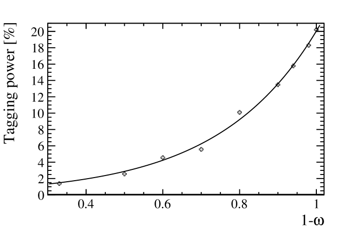
Figure 1: Tagging power as a function of the correct particle identification rate $1-\omega$.

2.5 Decay time resolution

The resolution of $\phi_{s}$ is affected by the inaccurate determination of the decay time. The proper decay time of the $B_{s}$ is calculated from the vertex position and transverse momentum of the $B_{s}$ as:

$$t_{xy}=\frac{ml_{xy}}{p_{\mathrm{T}}},$$

where $l_{xy}=\sqrt{x^{2}+y^{2}}$ is the vertex position in the transverse plane.

Figure 2 shows the distribution of the difference between $t_{\text{reco}}$ and $t_{\text{sim}}$, where $t_{\text{reco}}$ is the proper decay time calculated from the reconstructed particle information, and $t_{\text{sim}}$ is obtained with the Monte Carlo simulated particle information without considering the detector effects. The distribution is fitted using the sum of three Gaussian functions with the same mean value. The effective time resolution is combined as

$$\sigma_{\text{eff}}=\sqrt{-\frac{2}{\Delta m_{s}^{2}}\ln(\sum_{i}f_{i}e^{-\frac{1}{2}\sigma_{i}^{2}\Delta m_{s}^{2}})},$$

where $f_{i}$ and $\sigma_{i}$ are fraction and width of the i-th Gaussian function. The effective resolution of the decay time is ${4.7~{}\mathrm{fs}}$.

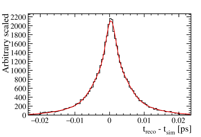
Figure 2: distribution of $t_{\text{reco}}-t_{\text{sim}}$. The distribution is fitted with the sum of three Gaussian functions with equal mean.

3 Results and discussion

Table 1: Parameters table of factors to calculate the resolution. The terms with $*$ means that the factor is insensitive to the resolution of $\Gamma_{s}$ and $\Delta\Gamma_{s}$.

	LHCb (HL-LHC)	CEPC (Tera-Z)	CEPC/LHCb
$b\bar{b}$ statics	$43.2\times 10^{12}$	$0.152\times 10^{12}$	1/284
Acceptance$\times$efficiency	$7\%$	$75\%$	10.7
Br	$6\times 10^{-6}$	$12\times 10^{-6}$	2
Flavour tagging∗	$4.7\%$	$20\%$	4.3
Time resolution∗ ($\exp({-\frac{1}{2}\Delta m_{s}^{2}\sigma_{t}^{2}})^{2}$)	$0.52$	$1$	1.92
scaling factor $\xi$	0.0014	0.0019	0.8
$\sigma(\phi_{s})$	$3.3~{}\mathrm{mrad}$	$4.3~{}\mathrm{mrad}$

Simulations show that in future $Z$-factories, the proper decay time resolution can reach $4.7~{}\mathrm{fs}$, the detector acceptance$\times$efficiency can be as good as $75\%$, and the flavor tagging power can be $20\%$. Assuming the future $Z$-factory operating in Tera-$Z$ mode (i.e., $10^{12}$ $Z$), the scaling factor $\xi_{FE}$ is $0.0019$. The expected $\phi_{s}$ resolution is $\sigma(\phi_{s},\text{FE})=\xi_{\text{FE}}\times\sigma(\phi_{s},\text{LHCb})/\xi_{\text{LHCb}}=4.3~{}\mathrm{mrad}$, which is competitive to $3.3~{}\mathrm{mrad}$, the expected $\phi_{s}$ measurement resolution of LHCb at the HL-LHC.

The $\Gamma_{s}$ and $\Delta\Gamma_{s}$ are dependent weakly on tagging power and decay time resolution. The 4.3 times better flavor tagging power and 1.92 times better time resolution factor of CEPC, in contrast to $\phi_{s}$, have no effects on these observables. The estimated resolution is $0.24~{}\mathrm{ns^{-1}}$ for $\Delta\Gamma_{s}$ and $0.072~{}\mathrm{ns^{-1}}$ for $\Gamma_{s}$. The measured resolution of $\Gamma_{s}-\Gamma_{d}=0.0024~{}\mathrm{ps^{-1}}$LHCb:2019nin is taken as the resolution of $\Gamma_{s}$.

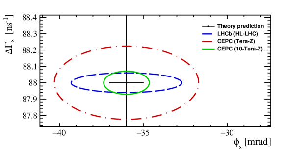
Figure 3: Expected confidential region ($68\%$ confidential level) of $\Delta\Gamma_{s}-\phi_{s}$. The black point is the Standard Model prediction from CKMFitter group Charles:2015gya and HQE theory calculation HQE . The uncertainty of $\Delta\Gamma_{s}$ is $6~{}\mathrm{ns}^{-1}$. The dot dash red curve represents the Tera-$Z$ CEPC. The dash blue curve represents the LHCb on High-Luminosity LHC. The solid green curve represents the 10-Tera-$Z$ CEPC. All the circles are centered at the standard model central value.

Figure 3 shows the expected confidential range ($68\%$ confidential level) of $\Delta\Gamma_{s}-\phi_{s}$. The black dot is the prediction of the standard model from CKMFitter group Charles:2015gya and HQE theory calculation HQE . The dot dash red curve and the dash blue curve represent the expected precision of Tera-$Z$ CEPC and LHCb at the HL-LHC. The solid green curve shows the expected precision of 10-Tera-$Z$ CEPC. The $\phi_{s}$ resolution at the 10-Tera-$Z$ CEPC can reach the current precision of SM prediction. All the future experiments measurements of $\Delta\Gamma_{s}$ can provide strigent constraints on the HEQ theory.

As shown in Table 1, the statistical disadvantage of the Tera-$Z$ $Z$ factory can be compensated with a much cleaner environment, good particle identification, and accurate track and vertex measurement. Without the benefits of flavor tagging and time resolution, the $\Gamma_{s}$ and $\Delta\Gamma_{s}$ resolution is much worse than expected for the LHC at high-luminosity. Only with the 10-Tera-$Z$ $Z$ factory can the expected resolution of $\Delta\Gamma_{s}$ and $\Gamma_{s}$ be competitive.

Particle identification is critical. Tagging performance degrades rapidly when particles are incorrectly identified. With the particle identification information, the different hadrons can be distinguished to achieve a cleaner event selection. A good vertex reconstruction is required to rule out combinatorial backgrounds. The current decay time resolution is good enough. A better time resolution can not improve the precision of $\phi_{s}$.

Appendix A Appendix

The dependent of $\sigma(\phi_{s})$, $\sigma(\Delta\Gamma_{s})$ and $\sigma(\Gamma_{s})$ on the time resolution and tagging power is investigated with toy Monte Carlo simulation. Figure 4 shows the varying of resolution for $\phi_{s}$ and $\Gamma_{s}$ as a function of the tagging power and decay time resolution. The ratio to the baseline resolution is plotted. The baseline resolution is with the parameters $\sigma_{t}=4.7~{}\mathrm{fs}$ and $p=20\%$. The red line with square marker and the blue line with triangle marker represent the resolution from toy Monte Carlo simulation respectively. The black line with circle marker represents the resolution from the analytical formula. The resolution ratio of $\Gamma_{s}$ is almost the same to the resolution ratio of $\Delta\Gamma_{s}$.

The simulation provides a validation of the formula

$$\sigma(\phi_{s})\propto\exp({-\frac{1}{2}\Delta m_{s}^{2}\sigma_{t}^{2}})$$

and

$$\sigma(\phi_{s})\propto\sqrt{p},$$

and it also provides a validation that the resolution of $\Gamma_{s}$ and $\Delta\Gamma_{s}$ are insensitive to the time resolution and tagging power.

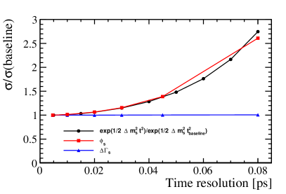
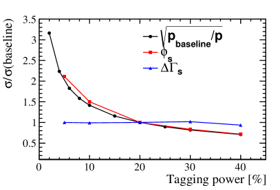
Figure 4: The varying of resolution for $\phi_{s}$ and $\Gamma_{s}$ as a function of the decay time resolution (left) and tagging power resolution (right). The ratio to the baseline resolution is plotted. The baseline resolution is with the parameters $\sigma_{t}=4.7~{}\mathrm{fs}$ and $p=20\%$. The red line with square marker and the blue line with triangle marker represent the resolution from toy Monte Carlo simulation respectively. The black line with circle marker represents the resolution from the analytical formula.

References

- (1) J. Charles et al., Current status of the Standard Model CKM fit and constraints on New Physics, Phys. Rev. D 91 (2015) 073007 [1501.05013].
- (2) UTfit collaboration, The Unitarity Triangle Fit in the Standard Model and Hadronic Parameters from Lattice QCD: A Reappraisal after the Measurements of Delta m(s) and BR(B — tau nu(tau)), JHEP 10 (2006) 081 [hep-ph/0606167].
- (3) Particle Data Group collaboration, Review of Particle Physics, PTEP 2020 (2020) 083C01.
- (4) M. Neubert, B decays and the heavy quark expansion, Adv. Ser. Direct. High Energy Phys. 15 (1998) 239 [hep-ph/9702375].
- (5) ATLAS collaboration, Measurement of the -violating phase in decays in ATLAS at 13 TeV, Eur. Phys. J. C 81 (2021) 342 [2001.07115].
- (6) ATLAS collaboration, Flavor tagged time-dependent angular analysis of the decay and extraction of s and the weak phase in ATLAS, Phys. Rev. D 90 (2014) 052007 [1407.1796].
- (7) CDF collaboration, Measurement of the Bottom-Strange Meson Mixing Phase in the Full CDF Data Set, Phys. Rev. Lett. 109 (2012) 171802 [1208.2967].
- (8) CMS collaboration, Measurement of the CP-violating weak phase and the decay width difference using the B(1020) decay channel in pp collisions at 8 TeV, Phys. Lett. B 757 (2016) 97 [1507.07527].
- (9) D0 collaboration, Measurement of the CP-violating phase using the flavor-tagged decay in 8 fb-1 of collisions, Phys. Rev. D 85 (2012) 032006 [1109.3166].
- (10) LHCb collaboration, Resonances and violation in and decays in the mass region above the , JHEP 08 (2017) 037 [1704.08217].
- (11) LHCb collaboration, Updated measurement of time-dependent \it CP-violating observables in decays, Eur. Phys. J. C 79 (2019) 706 [1906.08356].
- (12) LHCb collaboration, Measurement of the -violating phase in decays, Phys. Rev. Lett. 113 (2014) 211801 [1409.4619].
- (13) LHCb collaboration, First study of the CP -violating phase and decay-width difference in decays, Phys. Lett. B 762 (2016) 253 [1608.04855].
- (14) LHCb collaboration, Measurement of the -violating phase from decays in 13 TeV collisions, Phys. Lett. B 797 (2019) 134789 [1903.05530].
- (15) C.S. Group et al., Cepc conceptual design report: Volume 2-physics & detector, arXiv preprint arXiv:1811.10545 (2018) .
- (16) W.K. et al., Simulating Multi-Particle Processes at LHC and ILC, 2011.
- (17) T. Sjöstrand, Pythia, .
- (18) S. Agostinelli, J. Allison, K.a. Amako, J. Apostolakis, H. Araujo, P. Arce et al., Geant4-a simulation toolkit, Nuclear instruments and methods in physics research section A: Accelerators, Spectrometers, Detectors and Associated Equipment 506 (2003) 250.