Electric Current Induced by Microwave Stark Effect of Electrons on Liquid Helium
Abstract
We propose a frequency-mixed effect of Terahertz (THz) and Gigahertz (GHz) electromagnetic waves in the cryogenic system of electrons floating on liquid helium surface. The THz wave is near-resonant with the transition frequency between the lowest two levels of surface state electrons. The GHz wave does not excite the transitions but generates a GHz-varying Stark effect with the symmetry-breaking eigenstates of electrons on liquid helium. We show an effective coupling between the inputting THz and GHz waves, which appears at the critical point that the detuning between electrons and THz wave is equal to the frequency of GHz wave. By this coupling, the THz and GHz waves cooperatively excite electrons and generate the low-frequency ac currents along the perpendicular direction of liquid helium surface to be experimentally detected by the image-charge approach [Phys. Rev. Lett. 123, 086801 (2019)]. This offers an alternative approach for THz detections.
pacs:
73.20.-rElectron states at surfaces and interfaces and 42.50.CtQuantum description of interaction of light and matter; related experiments and 42.50.-pQuantum optics and 85.35.BeQuantum well devices (quantum dots, quantum wires, etc.)1 Introduction
Electrons floating on liquid helium surface have been considered as an alternative physical system to implement quantum computation Platzman1967 ; PhysRevX.6.011031 ; PhysRevLett.89.245301 ; PhysRevB.67.155402 ; PhysRevLett.107.266803 ; PhysRevLett.101.220501 ; PhysRevLett.105.040503 ; Monarkha2019 ; PhysRevLett.124.126803 ; Spin ; PhysRevB.86.205408 . Sommer first noticed that there is a barrier at the surface of liquid helium that prevents electrons from entering its interior PhysRevLett.12.271 . Therefore, in addition to the attractive force of image charge in liquid helium, the surface electron forms a one-dimensional (1D) hydrogen atom above liquid helium surface RevModPhys.46.451 ; PhysRevLett.32.280 ; PhysRevB.13.140 . The two lowest levels of the 1D hydrogen atoms have been proposed to encode the qubits, which have good scalability due to the strong Coulomb interactions between electrons Platzman1967 . However, the single electron detection is still very difficult in experiments. Recently, E. Kawakami et.al. have used the image-charge approach to experimentally detect the Rydberg states of surface electrons on liquid helium PhysRevLett.123.086801 . Compared with the conventional microwave absorption method, this method may be more effective to detect the quantum state of surface electrons Elarabi2021 ; PhysRevLett.126.106802 .
The transition frequency between the lowest two levels of surface electrons is in the regime of Terahertz (THz) and therefore has perhaps applications in the fields of THz detection and generation. The THz spectrum is between the usual microwave and infrared regions, and has many practical applications NaturePhotonics , such as THz wireless communication THZ-Wireless Communication , astronomical observation EPJP-astronomy , Earth’s atmosphere monitoring watter , and the food safety food . Specially, in biological and medical fields biology ; APL , THz imaging have smaller damages in body than X-ray, but higher resolution than mechanical supersonic waves.
In this paper, we show a frequency-mixed effect of the THz and the Gigahertz (GHz) electromagnetic waves in the system of electrons floating on liquid helium. This effect could be applied to detect THz radiation. In our mixer, the inputting THz wave near-resonantly excites the transition between the lowest two levels of surface state electrons. The GHz wave does not excite the transitions but generates a GHz-varying Stark effect. This Stark effect has no counterpart in the system of natural atoms. The effective coupling between natural atoms and microwaves needs either the atomic high Rydberg states of Jing2020 or the magnetic coupling (with the strong microwave inputting). Here, the surface-bound states of electrons are symmetry broken due to the barrier at the liquid surface, and therefore the GHz wave can cause a GHz-varying energy gap of electrons on liquid helium by the lowest order electric dipole interaction. Specially, we find an effective coupling between the inputting THz and GHz waves, which appears at the frequencies condition that the detuning between electrons and THz wave is equal to the frequency of GHz wave. By this coupling, the THz and GHz waves cooperatively excite electrons and generate the low-frequency ac currents along the perpendicular direction of liquid helium surface to be experimentally detected by using the image-charge approach PhysRevLett.123.086801 ; Elarabi2021 ; PhysRevLett.126.106802 .
2 The Hamiltonian
Due to the image potential and the barrier at liquid helium surface, electronic motion along the perpendicular direction of liquid helium surface can be treated as a 1D hydrogen atom. Its energy level is well known as PhysRevA.61.034901 ; PhysRevA.80.055801
| (1) |
with . The is the charge of an electron, is the electronic mass, and the dielectric constant of liquid helium. Numerically, the transition frequency between the lowest two levels is THz (corresponding to a wavelength of mm). The eigenfunction of the above energy level reads
| (2) |
with being the Bohr radius, and
| (3) |
the Laguerre polynomial.
Considering only the lowest two levels in Eq. (1), the Hamiltonian of an electron driven by the classical electromagnetic fields can be written as
| (4) |
with the bare-atomic part
| (5) |
and the electric dipole interaction
| (6) |
Here, is the electric dipole moment, and the two-level operator with . Note that and for the wave function (2). On electric field E, we first consider the case of two-wave mixing, i.e.,
| (7) |
with THz and GHz. The and are the amplitudes of the inputting THz and GHz waves. The and are their initial phases, respectively.
Limiting within the usual rotating-wave approximation, the works only on the first two terms in Eq. (6), and works only on the last two terms in Eq. (6). Then, the Hamiltonian (4) in the usual interacting picture [defined by the unitary operator ] can be approximately written as
| (8) |
with the time-dependent coupling frequencies , , and . The and are due to the symmetry-breaking eigenstates of electron floating on liquid helium surface. The is the standard Rabi frequency of electric dipole transition, and is the detuning between the THz wave and the resonant frequency of electronic transition . For the analyzable effects of THz and GHz mixing, we apply another unitary transformation to the electronic states. Here,
| (9) |
| (10) |
and
| (11) |
As a consequence, Hamiltonian (8) in the new interacting picture reads
| (12) |
with
| (13) |
and
| (14) |
According to the well-known Jacobi-Anger expansion, we approximately write (13) as
| (15) | ||||
with being the Bessel function of the first kind. Considering the field strength of GHz wave is weak, i.e., , and supposing the frequency condition is satisfied, then the Eq. (15) reduces to
| (16) |
with the rotating-wave approximation. As a consequence, Hamiltonian (12) reduces to
| (17) |
which generates the standard Rabi oscillation at frequency . This Hamiltonian implies that the electrons floating on liquid helium may be applied as a frequency-mixer to generate the low frequency signal with .
3 The master equation
We use the standard master equation of classical electromagnetic waves interacting with the two-levels system RevModPhys.77.633 to numerically solve the dynamical evolution of surface state electrons on liquid helium. The master equation reads
| (18) |
with the decoherence operator
| (19) | ||||
Above, , with and . The is the so-called density matrix elements of the two-levels system. The is the spontaneous decay rate of . The and describe the energy-conserved dephasing RevModPhys.77.633 . It is worth to note that the unitary operator made for the Hamiltonian transformation (8) (12) does not change the formation of master equation. The proofs are detailed as follows.
Firstly, we rewrite the density operator as with , and rewrite the Hamiltonian (8) as , with and . Our unitary operator obeys the commutation relation , so
| (20) | ||||
Secondly, according to the original master equation (18), we have
| (21) | ||||
and where is nothing but Eq. (12). The decoherence operator obeys the following equation
| (22) |
because , , and , with and .
Finally, comparing Eqs. (20) and (21), we find
| (23) |
and get the master equation in interaction picture
| (24) |
which has the same form as that of (18). Moreover, using the above approach one can easily find that the usual unitary transformation also does not change the form of master equation. Compared with the original Hamiltonian (8), the Hamiltonian in interacting pictures is more clear to show the frequency-matching condition between electron and microwaves. While, the Hamiltonian , as proved above, is also valid to numerically (exactly) solve the master equation.
4 The results and discussion
According to master equation (24), we get the following equations for density matrix elements,
| (25) | ||||
| (26) |
In the experimental systems PhysRevLett.123.086801 ; Elarabi2021 ; PhysRevLett.126.106802 , the liquid helium surface (with the surface-state electrons) is set approximately midway between two plates of a parallel-plate capacitor, and the induced image charges on one of the capacitor plates is described by . The is the charge of electrons on liquid helium surface, and the average height of these electrons. The is the distance between the two parallel plates of capacitor. In terms of density matrix elements, the expectation value in Schrödinger picture is described by
| (27) | ||||
Numerically, the transition matrix elements are , , and . Note that, the term in Eq. (27) is due to the standard unitary transformation in Sec. 2 applied for the interacting Hamiltonian (8), and is due to the second unitary transformation employed for Hamiltonian (12). Specially, the term rapidly vibrates with the intrinsic frequencies of two-level electrons on liquid helium and generates the THz radiation.
According to our rotating-wave approximated Hamiltonian (17), the density matrix elements and vibrate with the Rabi frequency . The rotating-wave terms in Eq. (15), such as , vibrate with much higher frequencies than , but has small amplitude as shown in Fig. 1. The frequency distribution functions in Fig. 1 are obtained by numerically solving the following Fourier transforms
| (28) |
| (29) |
and
| (30) |
The is the amplitude of a harmonic vibrational component in function , with being the dimensionless time. The frequency of this component (harmonic vibration) is , with being the dimensionless coefficient. The explanations for and are similar.
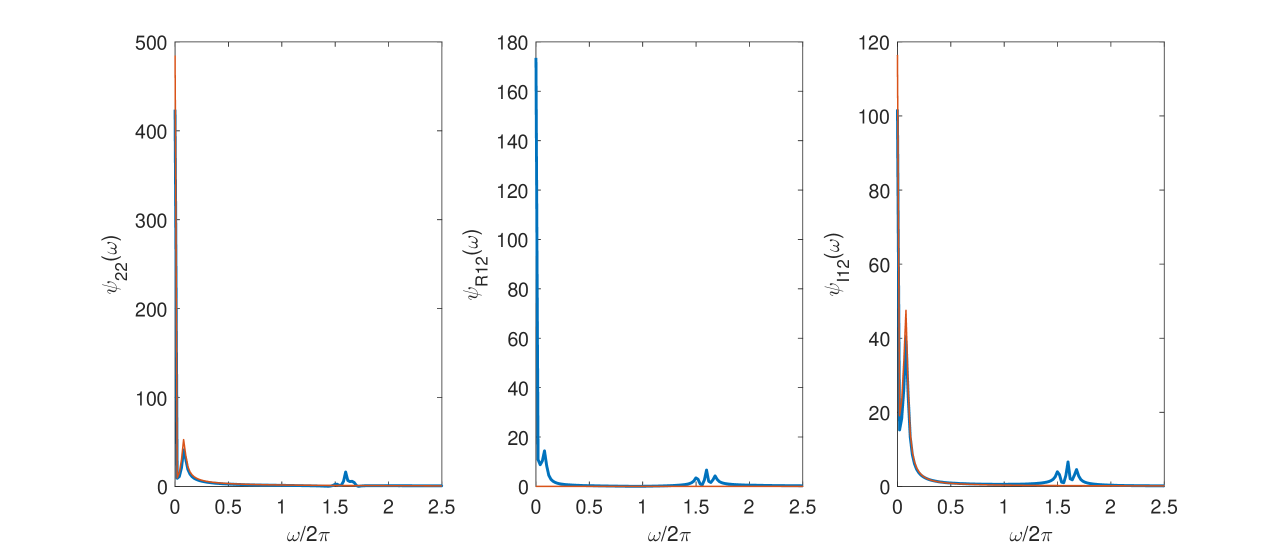
Due to the negligible components of high frequency vibrations in , see Fig. 1, the off-diagonal term in Eq. (27) is still the THz vibration due to the characteristic term . The THz waves travel in free space, and thus the off-diagonal term in Eq. (23) is negligible for the microwave circuit experiments PhysRevLett.123.086801 ; Elarabi2021 ; PhysRevLett.126.106802 , and then the formula of the vibrational image charge reduces to
| (31) |
As to was mentioned at the beginning of this paper, the GHz wave can not directly excite the transition , the THz wave acts as a trigger to start the system work. This mechanism is showed in Fig.2, where the detuning between THz wave and electron is set at . The electric field strength and the frequency of the GHz microwave are set at V/cm and GHz, respectively.
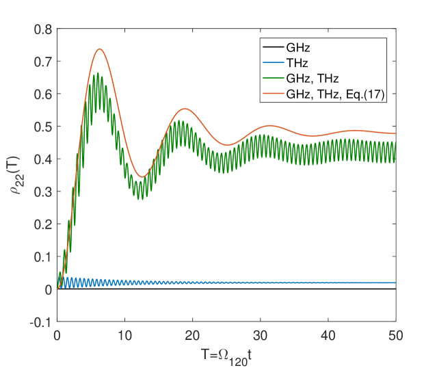
In Fig. 2, the red line is the solution of the rotating-wave approximated Hamiltonian , i.e., Eq. (17). This low frequency signal is the damped one because the Hamiltonian is time-independent. For a time-independent Hamiltonian, the master equation has the steady-state solution, i.e., with ZHANG201412 . The same phenomenon can be found in the blue line in Fig. 2, which describes the excitation by THz wave only. In this case, the Hamiltonian (12) reduces to with . This Hamiltonian can be also written in a time-independent form, i.e., , by simply employing the unitary transformation of . So, the blue line is also the damped one. Readers may notice that the blue line vibrates much faster than the red line. This can be simply explained by the analytic solution of Schrödinger equation of . The solution says the electron excitation probability with the frequency . In the large detuning regime, i.e., , the vibrational frequency is obviously larger than the standard Rabi frequency , but the amplitude is small (the rotating-wave effect).
The green line is the numerical solution of Hamiltonian (12) without the rotating-wave approximation. Then, the vibration has not only the low frequency component but also the high frequency component. In this case, the persistent oscillation exists, because Hamiltonian (12) is associated with the rotating-wave terms and can not be written in the time-independent form by any unitary transformation, as well as the original Hamiltonian (8). However, the frequency of persistent oscillation is on the order of the inputting GHz wave and is not the usable signal that a frequency-mixer should produce. Thus we suggest using the low frequency signal predicted by the red line to detect the THz inputting, although the signal is the damped one. This means that a pulsed source of GHz microwave is needed. Furthermore, we note that the above detuning is set at . This condition may not exactly satisfy in the practical experiments, and therefore the effective Hamiltonian (17) becomes
| (32) |
with . The solution of this Hamiltonian is similar to that of , but can still generate the low-frequency signal with and .
Finally, we describe a possibility to generate the persistent signal, i.e., monitor THz incoming online. Based on the above discussion, we apply another GHz wave to the electrons. Such that the inputting field (7) extends to
| (33) |
and consequently, the Eqs. (12) and (13) become, respectively,
| (34) |
and
| (35) |
The derivation for is similar to that of parameter in Eq. (14). Considering also , we have
| (36) |
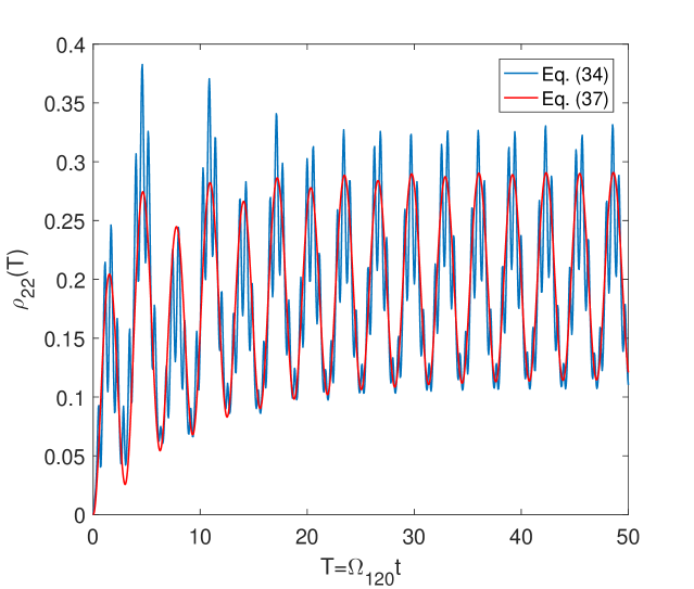
by employing the rotating-wave approximation again, and where and . Furthermore, considering the typical case that and , such that the effective Hamiltonian (17) becomes,
| (37) |
Due to the small detuning , this Hamiltonian can be never written in a time-independent form by any unitary transformations, and thereby the master equation has no steady-state solution. This causes the persistently oscillating charge, as shown in Fig. 3, which serves as a source for the low-frequency microwave outputting and could be applied to realize the real-time detection of THz incoming.
5 Conclusion
In summary, we have studied the frequency-mixed effects of THz and GHz waves in the cryogenic system of electrons floating on liquid helium. Different from the natural atoms, the transition frequency between the lowest two levels of electrons floating on liquid is in the THz regime. Moreover, the surface-state of electrons is symmetry breaking due to the barrier at the liquid surface. Therefore, both of THz and GHz waves can effectively drive the electrons via the electric dipole interaction. Specifically, the THz wave near-resonantly excites the transition between the lowest two levels of surface-bound electrons, the GHz wave does not excite the transition but generates the GHz-varying Stark effect. Using the unitary transformation approach and the rotating-wave approximation, we found an effective Hamiltonian (17) of two-wave mixing with the detuning , which could generate the significant ac current of frequency much lower than GHz, as shown in Fig. 2. The Hamiltonian is time-independent, so the generated low-frequency signal is the damped one due to the decay of surface-state electrons. To generate the persistent low-frequency signal, the time-dependent Hamiltonian is required, for example, the effective Hamiltonian (37) proposed for the case of three-wave mixing.
Acknowledgements: This work was supported by the National Natural Science Foundation of China, Grants No. 12047576, and No. 11974290.
Data Availability Statement: The data generated or analyzed during this study are included in this published article.
References
- (1) P.M. Platzman, M.I. Dykman, “Quantum computing with electrons floating on liquid helium”, Science 284, 1967 (1999). https://doi.org/10.1126/science.284.5422.1967
- (2) G. Yang, A. Fragner, G. Koolstra, L. Ocola, D.A. Czaplewski, R.J. Schoelkopf, D.I. Schuster, “Coupling an ensemble of electrons on superfluid helium to a superconducting circuit”, Phys. Rev. X 6, 011031 (2016). https://doi.org/10.1103/PhysRevX.6.011031
- (3) E. Collin, W. Bailey, P. Fozooni, P.G. Frayne, P. Glasson, K. Harrabi, M.J. Lea, G. Papageorgiou, “Microwave saturation of the Rydberg states of electrons on helium”, Phys. Rev. Lett. 89, 245301 (2002). https://doi.org/10.1103/PhysRevLett.89.245301
- (4) M.I. Dykman, P.M. Platzman, P. Seddighrad, “Qubits with electrons on liquid helium”, Phys. Rev. B 67, 155402 (2003). https://doi.org/10.1103/PhysRevB.67.155402
- (5) F.R. Bradbury, M. Takita, T.M. Gurrieri, K.J. Wilkel, K. Eng, M.S. Carroll, S.A. Lyon, “Efficient clocked electron transfer on superfluid helium”, Phys. Rev. Lett. 107, 266803 (2011). https://doi.org/10.1103/PhysRevLett.107.266803
- (6) S. Mostame, R. Schtzhold, “Quantum simulator for the Ising model with electrons floating on a helium film”, Phys. Rev. Lett. 101, 220501 (2008). https://doi.org/10.1103/PhysRevLett.101.220501
- (7) D.I. Schuster, A. Fragner, M.I. Dykman, S.A. Lyon, R.J. Schoelkopf, “Proposal for manipulating and detecting spin and orbital states of trapped electrons on helium using cavity quantum electrodynamics”, Phys. Rev. Lett. 105, 040503 (2010). https://doi.org/10.1103/PhysRevLett.105.040503
- (8) Y. Monarkha, D. Konstantinov, “Magneto-oscillations and anomalous current states in a photoexcited electron gas on liquid helium”, J. Low Temp. Phys. 197, 208 (2019). https://doi.org/10.1007/s10909-019-02210-w
- (9) A.O. Badrutdinov, D.G. Rees, J.Y. Lin, A.V. Smorodin, D. Konstantinov, “Unidirectional charge transport via ripplonic polarons in a three-terminal microchannel device”, Phys. Rev. Lett. 124, 126803 (2020). https://doi.org/10.1103/PhysRevLett.124.126803
- (10) S.A. Lyon, “Spin-based quantum computing using electrons on liquid helium”, Phys. Rev. A 74, 052338 (2006). https://doi.org/10.1103/PhysRevA.74.052338
- (11) M. Zhang, L.F. Wei, “Spin-orbit couplings between distant electrons trapped individually on liquid helium”, Phys. Rev. B 86, 205408 (2012). https://doi.org/10.1103/PhysRevB.86.205408
- (12) W.T. Sommer, “Liquid helium as a barrier to electrons”, Phys. Rev. Lett. 12, 271 (1964). https://doi.org/10.1103/PhysRevLett.12.271
- (13) M.W. Cole, “Electronic surface states of liquid helium”, Rev. Mod. Phys. 46, 451 (1974). https://doi.org/10.1103/RevModPhys.46.451
- (14) C.C. Grimes, T.R. Brown, “Direct spectroscopic observation of electrons in image-potential states outside liquid helium”, Phys. Rev. Lett. 32, 280 (1974). https://doi.org/10.1103/PhysRevLett.32.280
- (15) C.C. Grimes, T.R. Brown, M.L. Burns, C.L. Zipfel, “Spectroscopy of electrons in image-potential-induced surface states outside liquid helium”, Phys. Rev. B 13, 140 (1976). https://doi.org/10.1103/PhysRevB.13.140
- (16) E. Kawakami, A. Elarabi, D. Konstantinov, “Image-charge detection of the Rydberg states of surface electrons on liquid helium”, Phys. Rev. Lett. 123, 086801 (2019). https://doi.org/10.1103/PhysRevLett.123.086801
- (17) A. Elarabi, E. Kawakami, D. Konstantinov, “Cryogenic amplification of image-charge detection for readout of quantum states of electrons on liquid helium”, J. Low Temp. Phys. 202, 456 (2021). https://doi.org/10.1007/s10909-020-02552-w
- (18) E. Kawakami, A. Elarabi, D. Konstantinov, “Relaxation of the excited Rydberg states of surface electrons on liquid helium”, Phys. Rev. Lett. 126, 106802 (2021). https://doi.org/10.1103/PhysRevLett.126.106802
- (19) M. Tonouchi, “Cutting-edge terahertz technology”, Nat. Photon. 1, 97 (2007). https://doi.org/10.1038/nphoton.2007.3
- (20) K. Huang, Z. Wang, “Terahertz terabit wireless communication”, IEEE Microw. Mag. 12, 108 (2011). https://doi.org/10.1109/MMM.2011.940596
- (21) L. Sabbatini, L. Pizzo, G. Dall’Oglio, “The brightness temperature of Mercury at 150 and 240 GHz”, Eur. Phys. J. Plus. 126, 99 (2011). https://doi.org/10.1140/epjp/i2011-11099-3
- (22) J.S. Melinger, Y. Yang, M. Mandehgar, D. Grischkowsky, “THz detection of small molecule vapors in the atmospheric transmission windows”, Opt. Express 20, 6788 (2012). https://doi.org/10.1364/OE.20.006788
- (23) S. Khushbu, M. Yashini, R. Ashish, C.K. Sunil, “Recent advances in Terahertz time-domain spectroscopy and imaging techniques for automation in agriculture and food sector”, Food Anal Methods 15, 498 (2022). https://doi.org/10.1007/s12161-021-02132-y
- (24) P.H. Siegel, “Terahertz technology in biology and medicine”, IEEE Trans Microw Theory Tech 52, 2438 (2004). https://doi.org/10.1109/TMTT.2004.835916
- (25) M. Nagel, P. Haring Bolivar, M. Brucherseifer, H. Kurz, A. Bosserhoff, R. Bttner, “Integrated THz technology for label-free genetic diagnostics”, Appl. Phys. Lett. 80, 154 (2002). https://doi.org/10.1063/1.1428619
- (26) M. Jing, Y. Hu, J. Ma, H. Zhang, L.j. Zhang, L.t. Xiao, S.t. Jia, “Atomic superheterodyne receiver based on microwave-dressed Rydberg spectroscopy”, Nat. Phys. 16, 911 (2020). https://doi.org/10.1038/s41567-020-0918-5
- (27) M.M. Nieto, “Electrons above a helium surface and the one-dimensional Rydberg atom”, Phys. Rev. A 61, 034901 (2000). https://doi.org/10.1103/PhysRevA.61.034901
- (28) M. Zhang, H.Y. Jia, L.F. Wei, “Jaynes-Cummings models with trapped electrons on liquid helium”, Phys. Rev. A 80, 055801 (2009). https://doi.org/10.1103/PhysRevA.80.055801
- (29) M. Fleischhauer, A. Imamoglu, J.P. Marangos, “Electromagnetically induced transparency: Optics in coherent media”, Rev. Mod. Phys. 77, 633 (2005). https://doi.org/10.1103/RevModPhys.77.633
- (30) M. Zhang, W.Z. Jia, L.F. Wei, “Frequency-doubled scattering of symmetry-breaking surface-state electrons on liquid helium”, Physica B Condens. Matter 432, 12 (2014). https://doi.org/10.1016/j.physb.2013.09.026