Neuroevolutionary Feature Representations for Causal Inference

Abstract

Within the field of causal inference, we consider the problem of estimating heterogeneous treatment effects from data. We propose and validate a novel approach for learning feature representations to aid the estimation of the conditional average treatment effect or cate. Our method focuses on an intermediate layer in a neural network trained to predict the outcome from the features. In contrast to previous approaches that encourage the distribution of representations to be treatment-invariant, we leverage a genetic algorithm that optimizes over representations useful for predicting the outcome to select those less useful for predicting the treatment. This allows us to retain information within the features useful for predicting outcome even if that information may be related to treatment assignment. We validate our method on synthetic examples and illustrate its use on a real life dataset.

1 Introduction

In this note, we aim to engineer feature representations to aid in the estimation of heterogeneous treatment effects. Specifically, we consider the following graphical model

(1)

where $X\in\mathbb{R}^{d}$ denotes a vector of features, $W\in\{0,1\}$ represents a boolean treatment, and $Y\in\mathbb{R}$ denotes the outcome. Suppose $(X_{i},W_{i},Y_{i})$ for $i=1,\dotsc,n$ are i.i.d. samples from a distribution $P$ respecting the graph (1). Within the potential outcomes framework [20, 27], we let $Y_{i}(0)$ denote the potential outcome if $W_{i}$ were set to $0$ and $Y_{i}(1)$ denote the potential outcome if $W_{i}$ were set to $1$. We wish to estimate the conditional average treatment effect (cate) defined by

$$\tau(x)=\mathbb{E}[Y(1)-Y(0)|X=x].$$ (2)

We impose standard assumptions that the treatment assignment is unconfounded, meaning that

$$\{Y_{i}(0),Y_{i}(1)\}\perp W_{i}\mid X_{i},$$

for all $i$, and random in the sense that

$$\epsilon<P(W_{i}=1|X_{i}=x_{i})<1-\epsilon$$

for all $i$, some $\epsilon>0$, and all $x_{i}\in\mathbb{R}^{d}$ in the support of $X_{i}$. These assumptions are jointly known as strong ignorability [26] and prove sufficient for the cate to be identifiable. Under these assumptions, there exist well-established methods to estimate the cate from observed samples (see section 2.1 for a discussion) that then allow us to predict the expected individualized impact of an intervention for novel examples using only their features [22]. Viewing these approaches as black box estimators, we aim to learn a mapping $\Phi:\mathbb{R}^{d}\to\mathbb{R}^{m}$ such that the estimate of the cate learned from the transformed training data $(\Phi(X_{i}),W_{i},Y_{i})$ is more accurate than an estimate learned on the original samples $(X_{i},W_{i},Y_{i})$. In particular, we desire a function $\Phi$ yielding a corresponding representation $\Phi(X)$ such that

1. $\Phi(X)$ is as useful as $X$ for estimating $Y$, and

2. among such representations, $\Phi(X)$ is least useful for estimating $W$.

In this way, we hope to produce a new set of features $\Phi(X)$ that retain all information relevant for predicting the outcome, but are less related to treatment assignment. We propose learning $\Phi$ as an intermediate layer in a neural network estimating a functional relationship of $Y$ given $X$. We apply a genetic algorithm [9] to a population of such mappings to evolve and select the one for which the associated representation $\Phi(X)$ is least useful for approximating $W$.

Feature representations are commonly used in machine learning to aid in the training of supervised models [2] and have been previously demonstrated to aid in causal modeling. Johansson, et al. [11, 29] viewed counterfactual inference on observational data as a covariate shift problem and learned neural network-based representations designed to produce similar empirical distributions among the treatment and control populations, namely $\{\Phi(X_{i})\}_{W_{i}=1}$ and $\{\Phi(X_{i})\}_{W_{i}=0}$. Li & Fu [16] and Yao, et al. [34] developed representations in a related vein designed to preserve local similarity. We generally agree with Zhang et al.’s [36] recent argument that domain invariance often removes too much information from the features for causal inference. In contrast to most previous approaches, we develop a feature representation that attempts to preserve information useful for predicting the treatment effect if it is also useful for predicting the outcome.

1.0.1 Outline.

We proceed as follows. In the next section, we describe methods for learning the cate from observational data and introduce genetic algorithms. In section 3, we describe our methodology in full. We then validate our method on artificial data in section 4 and on a publicly available experimental dataset in section 5, before concluding in section 6.

2 Related work

In the first part of this section, we discuss standard methods for learning the cate function from data. We will subsequently use these to test our proposed feature engineering methods in section 4. In the second part, we briefly outline evolutionary algorithms for training neural networks, commonly called neuroevolutionary methods.

2.1 Meta-learners

We adopt the standard assumptions of unconfoundedness and the random assignment of treatment effects that together constitute strong ignorability. Given i.i.d. samples from a distribution $P$ respecting (1) and these assumptions, there exist numerous meta-learning approaches that leverage an arbitrary regression framework (e.g., random forests, neural networks, linear regression models) to estimate the cate that we now describe.

S-learner.

The S-learner (single-learner) uses a standard supervised learner (regression model) to estimate $\mu(x,w)=\mathbb{E}[Y|X=x,W=w]$ from observation data and then predicts

$$\hat{\tau}_{S}(x)=\hat{\mu}(x,1)-\hat{\mu}(x,0)$$

where we use the standard hat notation to denote estimated versions of the underlying functions.

T-learner.

The T-learner (two-learner) estimates $\mu_{1}(x)=\mathbb{E}[Y(1)|X=x]$ from observed treatment data $\{(X_{i},Y_{i})\}_{W_{i}=1}$ and $\mu_{0}(x)=\mathbb{E}[Y(0)|X=x]$ from observed control data $\{(X_{i},Y_{i})\}_{W_{i}=0}$, and then predicts

$$\hat{\tau}_{T}(x)=\hat{\mu}_{1}(x)-\hat{\mu}_{0}(x).$$

X-learner.

The X-learner [14] estimates $\mu_{1}$ and $\mu_{0}$ as in the T-learner, and then predicts the contrapositive outcome for each training point. Next, the algorithm estimates $\tau_{1}(x)=\mathbb{E}[\tilde{D}_{i}^{1}\mid X=x]$ on $\{(X_{i},\tilde{D}_{i}^{1})\}_{W_{i}=1}$ where $\tilde{D}_{i}^{1}=Y_{i}-\hat{\mu}_{0}(X_{i})$ and $\tau_{0}(x)=\mathbb{E}[\tilde{D}_{i}^{0}\mid X=x]$ on $\{(X_{i},\tilde{D}_{i}^{0})\}_{W_{i}=0}$ where $\tilde{D}_{i}^{0}=\hat{\mu}_{1}(X_{i})-Y_{i}$. The X-learner then predicts

$$\hat{\tau}_{X}(x)=g(x)\hat{\tau}_{0}(x)+(1-g(x))\hat{\tau}_{1}(x)$$

where $g:\mathbb{R}^{d}\to[0,1]$ is a weight function. The creators of the X-learner remark that the treatment propensity function (3) often works well for $g$, as do the constant functions $1$ and $0$. In our implementation, we use $g(x)\equiv 1/2$.

Concerning this method, we note that it is also possible to directly estimate $\tau$ from

$$\{(X_{i},Y_{i}-\hat{\mu}_{0}(X_{i}))\}_{W_{i}=1}\cup\{(X_{i},\hat{\mu}_{1}(X_{i})-Y_{i})\}_{W_{i}=0}$$

or, using $\hat{\mu}(x,w)$ from the S-learner approach, with

$$\{(X_{i},Y_{i}-\hat{\mu}(X_{i},0))\}_{W_{i}=1}\cup\{(X_{i},\hat{\mu}(X_{i},1)-Y_{i})\}_{W_{i}=0}.$$

We find that these alternate approaches work well in practice and obviate the need to estimate or fix $g$.

R-learner.

Within the setting of the graphical model (1), we define the treatment propensity (sometimes called the propensity score) as

$$e(x)=P(W=1|X=x)$$ (3)

and the conditional mean outcome as

$$m(x)=\mathbb{E}[Y|X=x].$$ (4)

The R-learner [21] leverages Robinson’s decomposition [25] that led to Robin’s reformulation [24] of the cate function as the solution to the optimization problem

$$\tau(\cdot)=\operatorname*{\arg\min}_{\tau}\bigg{\{}\mathbb{E}_{(X,W,Y)\sim P}\bigg{[}\left\lvert\big{(}Y-m(X)\big{)}-\big{(}W-e(X)\big{)}\tau(X)\right\rvert^{2}\bigg{]}\bigg{\}}$$ (5)

in terms of the treatment propensity (3) and the conditional mean outcome (4). In practice, a regularized, empirical version of (5) is minimized via a two-step process: (1) cross-validated estimates $\hat{m}$ and $\hat{e}$ are obtained for $m$ and $e$, respectively, and then (2) the empirical loss is evaluated using folds of the data not used for estimating $\hat{m}$ and $\hat{e}$, and then minimized. The authors Nie & Wager note that the structure of the loss function eliminates correlations between $m$ and $e$ while allowing one to separately specify the form of $\tau$ through the choice of optimization method. In this paper, the only R-learner we use is the causal forest as implemented with generalized random forests [1] using the default options, including honest splitting [33].

2.2 Genetic and neuroevolutionary algorithms

Holland introduced genetic algorithms [9] as a nature-inspired approach to optimization. Generally speaking, these algorithms produce successive generations of candidate solutions. New generations are formed by selecting the fittest members from the previous generation and performing cross-over and/or mutation operations on them to produce new offspring candidates. Evolutionary algorithms encompass extensions and generalizations to this approach including memetic algorithms [18] that perform local refinements, genetic programming [7] that acts on programs represented as trees, and evolutionary programming [6] and strategies [23, 28] that operate on more general representations. When such methods are applied specifically to the design and training of neural networks, they are commonly known as neuroevolutionary algorithms. See Stanley et al. [31] for a comprehensive survey. In the next section, we describe a specific neuroevolutionary strategy for feature engineering.

3 Methodology

In this section, we describe how we form our feature mapping $\Phi:\mathbb{R}^{d}\to\mathbb{R}^{m}$. To generate a single candidate solution, we train a shallow neural network to predict $Y$ from $X$ and extract an intermediate layer of this network. Each candidate map created in this way should yield a representation as functionally useful for predicting $Y$ as $X$ is. We then iteratively evolve cohorts of parameter sets for such maps to create a representation that carries the least amount of useful information for predicting the treatment $W$.

3.1 Candidate solutions

We consider neural networks $f_{\Theta}:\mathbb{R}^{d}\to\mathbb{R}$ of the form

$$f_{\Theta}(x)=M_{2}\cdot a(M_{1}\cdot x+b_{1})+b_{2}$$ (6)

where $M_{1}\in\mathbb{R}^{m\times d}$, $M_{2}\in\mathbb{R}^{1\times m}$ are real-valued matrices (often called weights), $b_{1}\in\mathbb{R}^{m}$ and $b_{2}\in\mathbb{R}^{1}$ are vectors (often called biases), and $a$ is a nonlinear activation function applied component-wise. We let $\Theta=(M_{1},M_{2},b_{1},b_{2})$ denote the parameters for $f_{\Theta}$. Though $f_{\Theta}$ is decidedly not a deep neural network, we note that, as a neural network with a single hidden layer, it remains a universal function approximator in the sense of Hornik et al. [10]. Optimizing the network (6) in order to best predict $Y$ from $X$ seeks the solution

$$\Theta_{*}=\operatorname*{\arg\min}_{\Theta}\mathbb{E}\left\lvert Y-f_{\Theta}(X)\right\rvert^{2}.$$ (7)

Given parameters $\Theta$ for the network (6), we let $\Phi_{\Theta}:\mathbb{R}^{d}\to\mathbb{R}^{m}$ given by

$$\Phi_{\Theta}(x)=a(M_{1}\cdot x+b_{1})$$ (8)

denote the output of the hidden layer. We restrict to candidate feature mappings of this form. As these mappings are completely characterized by their associated parameters, we define a fitness function and evolutionary algorithm directly in terms of parameter sets $\Theta$ in the following subsections.

3.2 Fitness function

For parameters $\Theta$ near the optimum (7), we note that $\Phi_{\Theta}(X)$ should be approximately as useful as $X$ for learning a functional relationship with $Y$. However, for some values of $\Theta$, the mapped features $\Phi_{\Theta}(X)$ may carry information useful for predicting $W$, and for this reason we consider a network $g_{\Psi,\Theta}:\mathbb{R}^{d}\to[0,1]$ given by

$$g_{\Psi,\Theta}(x)=\sigma(M_{4}\cdot a(M_{3}\cdot\Phi_{\Theta}(x)+b_{3})+b_{4})$$ (9)

where $M_{3}\in\mathbb{R}^{k\times m}$ and $M_{4}\in\mathbb{R}^{1\times k}$ are weights, $b_{3}\in\mathbb{R}^{k}$ and $b_{4}\in\mathbb{R}$ are biases, $a$ is a nonlinear activation function applied component-wise, and $\sigma(x)=(1+\exp(-x))^{-1}$ denotes the sigmoidal activation function. In this case, $\Psi=(M_{3},M_{4},b_{3},b_{4})$ denotes the collection of tunable parameters. We define the fitness of a parameter set $\Theta$ to be

$$\mu(\Theta)=\min_{\Psi}\mathbb{E}\left\lvert W-g_{\Psi,\Theta}(X)\right\rvert^{2}.$$ (10)

In this way, we express a preference for representations $\Phi_{\Theta}(X)$ that are less useful for predicting $W$. For a schematic of these architectures, please see Figure 1.

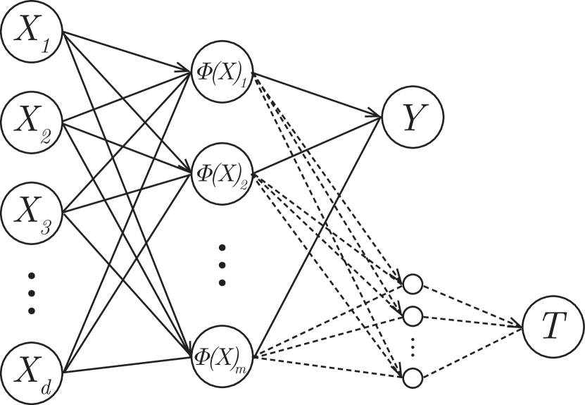
Figure 1: In this schematic, the arrows connecting the $X_{i}$ to the $\Phi(X)_{j}$ represent the map $\Phi_{\Theta}$ as in (8); these, in addition to the ones joining the $\Phi(X)_{j}$ to $Y$, represent $f_{\Theta}$ given explicitly in (6); and the original arrows along with the dashed arrows represent $g_{\Psi,\Theta}$ as in (9).

3.3 Evolutionary algorithm

We now describe a method to generate and evolve a cohort of candidate parameter sets $\Theta$ intended to seek a parameter set $\Theta_{*}$ such that $\Phi_{\Theta*}(X)$ is nearly as useful for predicting $Y$ as $X$ is and, among such representations, $\Phi_{\Theta*}(X)$ is least useful for predicting $W$.

Given training data $(X_{i},W_{i},Y_{i})\sim^{\text{i.i.d.}}P$ for $1\leq i\leq n$, we first partition the data into training and validation sets. We form an initial cohort of $c$ candidates independently as follows. For $1\leq j\leq c$, we randomly instantiate $\Theta_{j}$ using Glorot normal initialization [8] for the weights and zeros for the biases and then apply batch-based gradient descent on the training set to seek the solution to (7). In particular, we use the Adam optimizer [13] that maintains parameter-specific learning rates [5, cf. AdaGrad] and allows these rates to sometimes increase [35, cf. Adadelta] by adapting them using the first two moments from recent gradient updates. We use Tikhonov regularization [32] for the weights and apply a dropout layer [30] after the $a(x)=\tanh(x)$ activation functionto prevent overfitting.

For each constituent $\Theta_{j}$ in the cohort, we then initialize and train a network $g_{\Psi,\Theta_{j}}$ as in (9) to seek $\Psi_{j}=\operatorname*{\arg\min}_{\Psi}\mathbb{E}\left\lvert W-g_{\Psi,\Theta_{j}}(X)\right\rvert^{2}$ on the training set and then evaluate $\mathbb{E}\left\lvert W-g_{\Psi_{j},\Theta_{j}}(X)\right\rvert^{2}$ empirically on the validation set to estimate $\mu(\Theta_{j})$. We then use the $\ell$ fittest members of the current cohort to form a new cohort as follows. For each of the $\binom{\ell}{2}$ pairings, we apply Montana and Davis’s node-based crossover [17] method to the parameters $M_{1}$ and $b_{1}$ that we use to form $\Phi$. This amounts to forming a new $\Phi$ by randomly selecting one of the two parents and using that parent’s mapping for each coordinate. Thus, the new $M_{1}$ and $b_{1}$ are selected in a row-wise manner from the corresponding rows of the parents, and then the new $M_{2}$ and $b_{2}$ are randomly initialized and a few steps of optimization are performed to form the offspring candidate. The next generation then consists of the best performing candidate from the previous generation, $\binom{\ell}{2}$ candidates formed by crossing the best $\ell$ candidates of the previous generation, and $c-1-\binom{\ell}{2}$ entirely new candidates generated from scratch.

Data: training $\mathcal{T}=\{(X_{i},W_{i},Y_{i})\}_{i\in T}$ and validation $\mathcal{V}=\{(X_{i},W_{i},Y_{i})\}_{i\in V}$ datasets drawn i.i.d. from $P$ respecting the graphical model (1);

positive integer parameters: $c$ cohort size, $\ell$ number of members involved in forming the next generation, $g$ number of generations, $m$ dimensionality of the latent representation, and $k$ dimensionality of the final hidden layer in (9)

Result: parameterized function $\Phi_{\Theta_{*}}:\mathbb{R}^{d}\to\mathbb{R}^{m}$ such that models for the cate learned using the transformed training data $\{(\Phi(X_{i}),W_{i},Y_{i})\}_{i\in\mathcal{T}}$ perform better than those learned on the original dataset $\mathcal{T}$

for $j=1,\dotsc,c$ do

       Optimize a parameter set $\Theta_{j}$ to seek (7) on training batches from a random initialization;

      

end for

Form the first generation $\mathcal{G}_{1}=\{\Theta_{j}\}_{j=1,\dotsc,c}$;

for $t=2,\dotsc,g$ do #form the next generation

       Initialize new generation $\mathcal{G}_{t}=\{\operatorname*{\arg\max}_{\Theta\in\mathcal{G}_{t-1}}\mu(\Theta)\}$ with the best-performing candidate from the previous generation;

       for unique pairs $\{\Theta_{j},\Theta_{k}\}$ formed from the top $\ell$ candidates from $\mathcal{G}_{t-1}$ do #form new candidates using crossover

             Initialize $M_{1}\in\mathbb{R}^{m\times d}$ and $b_{1}\in\mathbb{R}^{m}$ as the $M_{1}$ and $b_{1}$ from $\Theta_{j}$;

             for $\kappa=1,\dotsc,m$ do

                   Let $\xi\sim\operatorname{Bernoulli}(1/2)$;

                   if $\xi=1$ then  replace the $\kappa$th row of $M_{1}$ and the $\kappa$th component of $b_{1}$ with those from $\Theta_{k}$;

                  

             end for

            Randomly initialize $M_{2}$ and $b_{2}$ and take optimization steps towards the solution to (7);

             Add $\Theta=(M_{1},M_{2},b_{1},b_{2})$ to $\mathcal{G}_{t}$

       end for

      while $\left\lvert\mathcal{G}_{t}\right\rvert<c$ do

             Optimize a parameter set $\Theta$ to seek (7) on training batches from a random initialization;

             Add $\Theta$ to $\mathcal{G}_{t}$

       end while

      

end for

Let $\Theta_{*}=\operatorname*{\arg\max}_{\Theta\in\mathcal{G}_{g}}\mu(\Theta)$;

return $\Phi_{\Theta_{*}}$ as in (8)

Algorithm 1 Neuroevolutionary Feature Engineering for Causal Inference

We summarize our approach using pseudo-code in Algorithm 1. All computation of the valuation function is done by training a network of the form (9) to minimize $\left\lvert W-g_{\Psi,\Theta}(X)\right\rvert^{2}$ on training batches and then approximating (10) by taking the empirical mean on the validation set.

3.4 Remark on linearity

Due to our choice of representation $\Phi$ in (8), after training the network (6) to optimize (7), we expect the relationship between the learned features $\Phi(X)$ and the outcome $Y$ to be approximately linear. In particular, we will have $Y\approx M_{2}\cdot\Phi(X)$ for $M_{2}$ as given in (6). For this reason, the causal meta-learners trained using a linear regression base learner may benefit more extensively from using the transformed features instead of the original features, especially in cases where the relationship between the original features and outcomes is not well-approximated as linear. We provide specific examples in the next section involving meta-learners trained with ridge regression.

3.5 Remark on our assumptions

In order to use the represented features $\Phi(X_{i})$ in place of the original features $X_{i}$ when learning the cate, we require that strong ignorability holds for the transformed dataset $(\Phi(X_{i}),W_{i},Y_{i})$, $i=1,\dotsc,n$. One sufficient, though generally not necessary, assumption that would imply strong ignorability is for $\Phi$ to be invertible on the support of $X$ [29, assumption 1]. Unconfoundedness would also be guaranteed if $\Phi(X)$ satisfied the backdoor condition with respect to $(W,Y)$ [22, section 3.3.1].

4 Ablation study on generated data

Due to the fundamental challenge of causal inference (namely, that the counterfactual outcome cannot be observed, even in controlled experiments), it is common practice to compare approaches to cate estimation on artificially generated datasets that allow the cate to be calculated directly for evaluative purposes. In this section, we perform experiments using two such data generation mechanisms from Nie & Wager’s paper [21] that we now describe. Both setups provide a joint distribution satisfying the graph (1). For the vector-valued random variable $X\in\mathbb{R}^{d}$, we let $X_{ij}$ denote $j$th component ($1\leq j\leq d$) of the $i$th sample ($1\leq i\leq n$). The specifics for both setups are given as follows.

4.0.1 Setup A.

For $\sigma>0$ and an integer $d>0$, we let

$$X_{i}\sim^{\text{i.i.d.}}\operatorname{Uniform}([0,1]^{d})\quad\text{and}\quad W_{i}\mid X_{i}\sim\operatorname{Bernoulli}(e(X_{i})),$$

where $e(X_{i})=\max\{0.1,\min\{\sin(\pi X_{i1}X_{i2}),0.9\}\}$ and

$$Y_{i}\mid X_{i},W_{i}\sim\mathcal{N}\big{(}b(X_{i})+(W_{i}-0.5)\tau(X_{i}),\sigma^{2}\big{)},$$

where $b(X_{i})=\sin(\pi X_{i1}X_{i2})+2(X_{i3}-0.5)^{2}+X_{i4}+0.5X_{i5}$ and $\tau(X_{i})=(X_{i1}+X_{i2})/2$. In this paper, we let $d=24$, $n=200$, and $\sigma=1$.

4.0.2 Setup C.

For $\sigma>0$ and an integer $d>0$, we let

$$X_{i}\sim^{\text{i.i.d.}}\mathcal{N}_{d}(\vec{0},I_{d\times d})\quad\text{and}\quad W_{i}\mid X_{i}\sim\operatorname{Bernoulli}(e(X_{i})),$$

where in this case $e(X_{i})=(1+\exp(X_{i2}+X_{i3}))^{-1}$ and

$$Y_{i}\mid X_{i},W_{i}\sim\mathcal{N}\big{(}b(X_{i})+(W_{i}-0.5)\tau(X_{i}),\sigma^{2}\big{)},$$

where now $b(X_{i})=2\log(1+\exp(X_{i1}+X_{i2}+X_{i3}))$ and $\tau(X_{i})=1$. In our example, we let $d=12$, $n=500$, and $\sigma=1$.

4.1 Comparison methodology

For each data generation method, we ran 100 independent trials. Within each trial, we simulated a dataset of size $n$ and randomly partitioned it into training, validation, and testing subsets at a 70%-15%-15% rate. We trained causal inference methods on the training set, using the validation data to aid the training of some base estimators for the meta-learners, and predicted on the test dataset. We then developed a feature map using the training and validation data as described in the previous section, applied this map to all features, and repeated the training and testing process using the new features.

To determine the impact of the fitness selection process, we also learned a feature transformation that did not make use of the fitness function at all. In effect, it simply generated a single candidate mapping and used it to transform all the features (without any cross-over or further mutation). Features developed in this way are described as “no fitness” in the tables that follow.

We compared the causal forest with default options (as found in R’s grf package), and the S-, T-, and X-learners as described in section 2.1 with two base learners. The first base learner is LightGBM [12], a boosted random forest algorithm that introduced novel techniques for sampling and feature bundling. The second is a cross-validated ridge regression model (as found in scikit-learn) that performs multiple linear regression with an $L^{2}$ normalization on the weights.

4.2 Results

We report results for setup A in Table 1 and results for setup C in Table 2. For both setups, we consider a paired t-test for equal means against a two-sided alternative (as implemented in Python’s scipy package). For setup A, we find that the improvement in MSE from using the transformed features in place of the original features corresponds to a statistically significant difference for the following learners: the causal forest ($p<0.001$), the S-learner with ridge regression ($p<0.001$), the T-learner with both LightGBM ($p<0.001$) and ridge regression ($p<0.001$), and the X-learner with both LightGBM ($p<0.001$) and ridge regression ($p<0.001$). For setup C, we again find significant differences for the causal forest ($p=0.023$), S-learner with LightGBM ($p=0.003$), T-learner with ridge regression ($p<0.001$) and X-learner with ridge regression ($p<0.001$).

In summary, we find that our feature transformation method improves the performance of multiple standard estimators for the cate under two data generation models.

learner	features	tr. 1	tr. 2	tr. 3	…	tr. 98	tr. 99	tr. 100	avg.
Causal forest	initial	0.488	0.161	0.042	…	0.207	0.212	0.592	0.175
	no fitness	0.305	0.050	0.035	…	0.048	0.068	0.353	0.114
	transformed	0.163	0.054	0.044	…	0.046	0.103	0.386	0.120
S-L. w/ LGBM	initial	0.121	0.055	0.191	…	0.048	0.059	0.323	0.149
	no fitness	0.171	0.111	0.089	…	0.149	0.098	0.395	0.140
	transformed	0.157	0.077	0.096	…	0.168	0.176	0.241	0.135
S-L. w/ Ridge	initial	0.257	0.038	0.032	…	0.048	0.067	0.290	0.093
	no fitness	0.202	0.038	0.037	…	0.039	0.046	0.249	0.079
	transformed	0.110	0.039	0.051	…	0.045	0.041	0.274	0.081
T-L. w/ LGBM	initial	0.574	0.351	0.691	…	0.448	0.198	1.189	0.666
	no fitness	0.647	0.516	0.596	…	0.393	0.303	0.669	0.536
	transformed	0.469	0.295	0.599	…	0.334	0.504	1.056	0.512
T-L. w/ Ridge	initial	0.763	0.254	0.888	…	0.916	0.260	0.553	0.745
	no fitness	0.257	0.177	0.103	…	0.237	0.114	0.574	0.333
	transformed	0.147	0.042	0.206	…	0.087	0.118	0.471	0.325
X-L. w/ LGBM	initial	0.339	0.207	0.309	…	0.394	0.134	0.811	0.411
	no fitness	0.497	0.225	0.230	…	0.161	0.128	0.493	0.335
	transformed	0.361	0.135	0.317	…	0.124	0.368	0.757	0.317
X-L. w/ Ridge	initial	0.643	0.221	0.702	…	0.798	0.240	0.470	0.630
	no fitness	0.247	0.145	0.097	…	0.197	0.110	0.540	0.289
	transformed	0.149	0.033	0.176	…	0.066	0.118	0.460	0.288

Table 1: Mean Squared Error (MSE) over 100 independent trials run using setup A. Algorithm 1 was run with parameters: cohort size $c=4$, progenitors $\ell=2$, number of cohorts $g=5$, representation dimensionality $m=20$, and fitness function parameter $k=10$.

learner	features	tr. 1	tr. 2	tr. 3	…	tr. 98	tr. 99	tr. 100	avg.
Causal forest	initial	0.002	0.062	0.016	…	0.023	0.008	0.071	0.035
	no fitness	0.004	0.027	0.028	…	0.046	0.006	0.047	0.029
	transformed	0.007	0.024	0.028	…	0.045	0.003	0.034	0.029
S-L. w/ LGBM	initial	0.247	0.244	0.279	…	0.222	0.190	0.202	0.226
	no fitness	0.173	0.207	0.207	…	0.214	0.164	0.198	0.211
	transformed	0.188	0.183	0.146	…	0.331	0.149	0.196	0.204
S-L. w/ Ridge	initial	0.000	0.024	0.017	…	0.004	0.012	0.005	0.015
	no fitness	0.000	0.016	0.017	…	0.005	0.012	0.005	0.015
	transformed	0.000	0.022	0.018	…	0.005	0.025	0.006	0.015
T-L. w/ LGBM	initial	0.771	0.482	0.833	…	0.490	0.538	0.424	0.567
	no fitness	0.587	0.543	0.593	…	0.491	0.766	0.537	0.551
	transformed	0.353	0.541	0.378	…	0.551	0.575	0.531	0.544
T-L. w/ Ridge	initial	0.143	0.260	0.189	…	0.173	0.148	0.124	0.178
	no fitness	0.049	0.164	0.096	…	0.145	0.106	0.093	0.125
	transformed	0.084	0.136	0.089	…	0.116	0.095	0.109	0.128
X-L. w/ LGBM	initial	0.286	0.216	0.474	…	0.282	0.247	0.275	0.313
	no fitness	0.348	0.236	0.361	…	0.318	0.377	0.254	0.313
	transformed	0.342	0.193	0.207	…	0.208	0.278	0.231	0.298
X-L. w/ Ridge	initial	0.129	0.241	0.170	…	0.156	0.136	0.114	0.166
	no fitness	0.039	0.142	0.081	…	0.119	0.099	0.079	0.109
	transformed	0.072	0.124	0.078	…	0.104	0.082	0.097	0.114

Table 2: Mean Squared Error (MSE) over 100 independent trials run using setup C. Algorithm 1 was run with $c=4$, $\ell=2$, $g=2$, $m=20$, and $k=10$.

5 Application to econometric data

In this section, we apply our feature engineering method to the LaLonde dataset [15, 4] chronicling the results of an experimental study on temporary employment opportunities. The dataset contains information from 445 participants who were randomly assigned to either an experimental group that received a temporary job and career counseling or to a control group that received no assistance. Features include age and education (in years), earnings in 1974 (in $, prior to treatment), and indicators for African-American heritage, Hispanic-American heritage, marital status, and possession of a high school diploma. We consider the outcome of earnings in 1978 (in $, after treatment).

We cannot determine true average treatment effects based on individual-level characteristics (i.e. the true cate values) for real life experimental data as we can with the synthetic examples of the previous section. Instead, we evaluate performance by comparing the average realized treatment effect and average predicted treatment effect within bins formed by sorting study participants according to predicted treatment effect as demonstrated in Figure 2. Applying the causal forest predictor to the original features results in a root mean square difference between the average predicted and realized treatment effects of 4729.51. If the transformed features are used instead, this discrepancy improves to 3114.82.

From a practical perspective, one may learn the cate in order to select a subset of people for whom a given intervention has an expected net benefit (and then deliver that intervention only to persons predicted to benefit from it). When we focus on the 20% of people predicted to benefit most from this treatment, we find that the estimated realized benefit for those chosen using the transformed features ($4732.89) is much greater than the benefit for those chosen using the original feature set ($816.92). This can be seen visually in Figure 2 by comparing the estimated realized average treatment effect for bin #5 (the rightmost bin) in both plots.

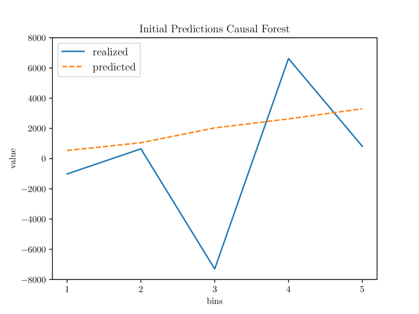
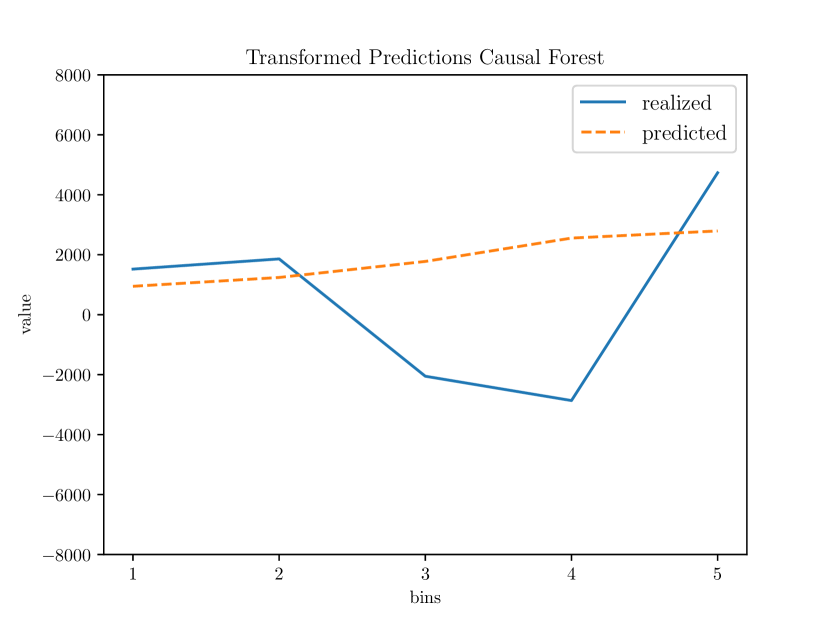
Figure 2: We plot estimated realized and predicted average treatment effects versus the quintiles of predicted treatment effect (5 bins) for a causal forest using (left) the initial features and (right) the features transformed using our method. In order to estimate realized treatment effect within each bin, we take the difference between the average outcome for persons randomly assigned to the experimental group and the average outcome for persons randomly assigned to the control group.

6 Conclusions

Causal inference, especially on real life datasets, poses significant challenges but offers a crucial avenue for predicting the impact of potential interventions. Learned feature representations help us to better infer the conditional average treatment effect, improving our ability to individually tailor predictions and target subsets of the general population. In this paper, we propose and validate a novel representation-based method that uses a neuroevolutionary approach to remove information from features irrelevant for predicting the outcome. We demonstrate that this method can yield improved estimates for heterogeneous treatment effects on standard synthetic examples and illustrate its use on a real life dataset. We believe that representational learning is particularly well-suited for removing extraneous information in causal models and we anticipate future research in this area.

Acknowledgements.

We would like to thank Binjie Lai, Yi-Hong Kuo, and Xiang Wu for their support and feedback. We are also grateful to the anonymous reviewers for their insights and suggestions.

Appendix 0.A Implementation details

All numerical experiments were performed with Python 3.7.7 and R 3.6.0. We used Python packages (versioning in parentheses) Keras (1.0.8), LightGBM (3.1.1), Matplotlib (3.3.4), Numpy (1.20.2), Pandas (1.2.4), rpy2 (2.9.4), Scikit-learn (0.24.2), Scipy (1.6.2), Tensorflow (2.0.0) with Intel MKL optimizations, and XGBoost (1.3.3), along with R package grf (1.2.0).

References

- [1] Athey, S., Tibshirani, J., Wager, S.: Generalized random forests. Ann. Statist. 47(2), 1148–1178 (2019)
- [2] Bengio, Y., Courville, A., Vincent, P.: Representation learning: A review and new perspectives. IEEE Trans. Pattern Anal. Mach. Intell. 35(8), 1798–1828 (2013)
- [3] Clevert, D.A., Unterthiner, T., Hochreiter, S.: Fast and accurate deep network learning by exponential linear units (elus). In: Int. Conf. Learn. Represent. (2016)
- [4] Dehejia, R.H., Wahba, S.: Causal effects in nonexperimental studies: Reevaluating the evaluation of training programs. J. Am. Stat. Assoc. 94(448), 1053–1062 (1999)
- [5] Duchi, J., Hazan, E., Singer, Y.: Adaptive subgradient methods for online learning and stochastic optimization. J. Mach. Learn. Res. 12, 2121–2159 (2011)
- [6] Fogel, L.: Autonomous automata. Ind. Res. Mag. 4(2), 14–19 (1962)
- [7] Forsyth, R.: Beagle – a Darwinian approach to pattern recognition. Kybernetes 10(3), 159–166 (1981)
- [8] Glorot, X., Bengio, Y.: Understanding the difficulty of training deep feedforward neural networks. In: Int. Conf. Artif. Intell. Stat. vol. 9, pp. 249–256 (2010)
- [9] Holland, J.H.: Adaptation in Natural and Artificial Systems. U. Michigan Press (1975)
- [10] Hornik, K., Stinchcombe, M., White, H.: Multilayer feedforward networks are universal approximators. Neural Netw. 2(5), 359–366 (1989)
- [11] Johansson, F., Shalit, U., Sontag, D.: Learning representations for counterfactual inference. In: Int. Conf. Mach. Learn. pp. 3020–3029 (2016)
- [12] Ke, G., Meng, Q., Finley, T., Wang, T., Chen, W., Ma, W., Ye, Q., Liu, T.Y.: LightGBM: A highly efficient gradient boosting decision tree. In: Adv. Neur. Inf. Proc. Sys. pp. 3146–3154 (2017)
- [13] Kingma, D.P., Ba, J.: Adam: A method for stochastic optimization. Int. Conf. Learn. Represent. (2015)
- [14] Künzel, S.R., Sekhon, J.S., Bickel, P.J., Yu, B.: Metalearners for estimating heterogeneous treatment effects using machine learning. Proc. Natl. Acad. Sci. 116(10), 4156–4165 (2019)
- [15] LaLonde, R.J.: Evaluating the econometric evaluations of training programs with experimental data. Am. Econ. Rev. 76(4), 604–620 (1986)
- [16] Li, S., Fu, Y.: Matching on balanced nonlinear representations for treatment effects estimation. In: Adv. Neur. Inf. Proc. Sys. pp. 930–940 (2017)
- [17] Montana, D.J., Davis, L.: Training feedforward neural networks using genetic algorithms. In: Int. Jt. Conf. Artif. Intell. pp. 762–767 (1989)
- [18] Moscato, P.: On evolution, search, optimization, genetic algorithms and martial arts: Towards memetic algorithms. Tech. Rep. C3P 826, Calif. Inst. Technol. (1989)
- [19] Nair, V., Hinton, G.: Rectified linear units improve restricted Boltzmann machines. In: Int. Conf. Mach. Learn. pp. 807–814 (2010)
- [20] Neyman, J.: Sur les applications de la théorie des probabilités aux experiences agricoles: Essai des principes. Rocz. Nauk Rol. 10, 1–51 (1923)
- [21] Nie, X., Wager, S.: Quasi-oracle estimation of heterogeneous treatment effects. Biometrika 108(2), 299–319 (2021)
- [22] Pearl, J.: Causality. Cambridge U. Press, 2nd edn. (2009)
- [23] Rechenberg, I.: Evolutionsstrategie: Optimierung technischer Systeme nach Prinzipien der biologischen Evolution. Ph.D. thesis, Technical U. Berlin (1970)
- [24] Robins, J.M.: Optimal structural nested models for optimal sequential decisions. In: 2nd Seattle Symp. Biostat. vol. LNS 179, pp. 189–326 (2004)
- [25] Robinson, P.M.: Root-n-consistent semiparametric regression. Econometrica 56(4), 931–954 (1988)
- [26] Rosenbaum, P.R., Rubin, D.B.: The central role of the propensity score in observational studies for causal effects. Biometrika 70(1), 41–55 (1983)
- [27] Rubin, D.: Estimating causal effects of treatments in randomized and nonrandomized studies. J. Educ. Psychol. 66(5), 688–701 (1974)
- [28] Schwefel, H.P.: Kybernetische Evolution als Strategie der experimentellen Forschung in der Strömungstechnik. Ph.D. thesis, Technical U. Berlin (1975)
- [29] Shalit, U., Johansson, F.D., Sontag, D.: Estimating individual treatment effect: generalization bounds and algorithms. In: Int. Conf. Mach. Learn. vol. 70, pp. 3076–3085 (2017)
- [30] Srivastava, N., Hinton, G., Krizhevsky, A., Sutskever, I., Salakhutdinov, R.: Dropout: A simple way to prevent neural networks from overfitting. J. Mach. Learn. Res. 15, 1929–1958 (2014)
- [31] Stanley, K., Clune, J., Lehmn, J., Miikkulainen, R.: Designing neural networks through neuroevolution. Nat. Mach. Intell. 1, 24–35 (2019)
- [32] Tikhonov, A.N.: Solution of incorrectly formulated problems and the regularization method. Proc. USSR Acad. Sci. 151(3), 501–504 (1963)
- [33] Wager, S., Athey, S.: Estimation and inference of heterogeneous treatment effects using random forests. J. Am. Stat. Assoc. 113(523), 1228–1242 (2018)
- [34] Yao, L., Li, S., Li, Y., Huai, M., Gao, J., Zhang, A.: Representation learning for treatment effect estimation from observational data. In: Adv. Neur. Inf. Proc. Sys. vol. 31, pp. 2633–2643 (2018)
- [35] Zeiler, M.D.: Adadelta: An adaptive learning rate method. ArXiv e-prints (2012)
- [36] Zhang, Y., Bellot, A., van der Schaar, M.: Learning overlapping representations for the estimation of individualized treatment effects. In: Int. Conf. Artif. Intell. Stats. (2020)
- [37] Zhao, H., des Combes, R.T., Zhang, K., Gordon, G.J.: On learning invariant representations for domain adaptation. In: Int. Conf. Mach. Learn. (2019)