Squeezing and quantum approximate optimization

Abstract

Variational quantum algorithms offer fascinating prospects for the solution of combinatorial optimization problems using digital quantum computers. However, the achievable performance in such algorithms and the role of quantum correlations therein remain unclear. Here, we shed light on this open issue by establishing a tight connection to the seemingly unrelated field of quantum metrology: Metrological applications employ quantum states of spin-ensembles with a reduced variance to achieve an increased sensitivity, and we cast the generation of such squeezed states in the form of finding optimal solutions to a combinatorial MaxCut problem with an increased precision. By solving this optimization problem with a quantum approximate optimization algorithm (QAOA), we show numerically as well as on an IBM Quantum chip how highly squeezed states are generated in a systematic procedure that can be adapted to a wide variety of quantum machines. Moreover, squeezing tailored for the QAOA of the MaxCut permits us to propose a figure of merit for future hardware benchmarks.

The Quantum Approximate Optimization Algorithm (QAOA) Farhi et al. (2014) is a promising approach for solving combinatorial optimization problems using digital quantum computers Torta et al. (2021); Headley et al. (2020). In this framework, combinatorial problems such as the MaxCut and MAX-SAT are mapped to the task of finding the ground state of an Ising Hamiltonian Lucas (2014); Liang et al. (2020); Lee et al. (2021). QAOA uses constructive interference to find solution states Streif and Leib (2019), and it has better performance than finite-time adiabatic evolution Wurtz and Love (2022). However, it remains an outstanding challenge to characterize the role of quantum effects such as entanglement in QAOA.

Here, we show how concepts from quantum metrology shed light onto the influence of squeezing and entanglement in the performance of QAOA. Illustratively, the connection is established through the insight that (a) the aim of QAOA is to obtain the ground state as precisely as possible, while (b) quantum metrology leverages entanglement between particles to generate states that permit precision beyond the capacities of any comparable classical sensor Pezzé and Smerzi (2009); Pezzè et al. (2018); Degen et al. (2017). For example, squeezed states can increase sensitivity for detecting phases Gross et al. (2010), magnetic fields Sewell et al. (2012), and gravitational waves Barsotti et al. (2018). The most sensitive states for phase estimation are Dicke states Dicke (1954); Pezzè et al. (2018), where all qubits are equally entangled. We substantiate this connection through numerically exact calculations and data gathered on IBM Quantum hardware with up to eight qubits. Our analysis shows how the search for an optimal solution to the MaxCut problem on a complete graph through QAOA generates a Dicke state, with squeezing and multipartite entanglement. Based on this, we propose the amount of squeezing generated as an application-tailored performance benchmark of QAOA. Our work thus further strengthens the intimate links between quantum metrology and quantum information processing Giovannetti et al. (2006); Omran et al. (2019); Marciniak et al. (2022); Arrazola et al. (2021).

In the rest of this paper, we first formally connect the QAOA to the generation of entangled squeezed states, which we then numerically illustrate. Next, we develop a benchmark tailored for QAOA based on squeezing. Finally, we assess the ability of superconducting qubits to run QAOA on fully connected problems while simultaneously creating Dicke states and estimate the number of entangled particles.

Combinatorial optimization on quantum computers. Universal quantum computers can address hard classical problems such as quadratic unconstrained binary optimization (QUBO), which is defined through

$$\min_{x\in\{0,1\}^{n}}x^{T}\Sigma x\quad\text{with}~{}\Sigma\in\mathbb{R}^{n\times n}.$$ (1)

In QAOA, the binary variables $x_{i}$ are mapped to qubits through $x_{i}=(1-z_{i})/2\rightarrow(1-\hat{Z}_{i})/2$, where $\hat{Z}_{i}$ is a Pauli spin operator with eigenstates $\ket{0}$ and $\ket{1}$. The result is an Ising Hamiltonian $\hat{H}_{C}$ whose ground state is the solution to Eq. (1) Lucas (2014). The standard QAOA then applies $p$ layers of the unitaries $\exp(-i\beta_{k}\hat{H}_{M})\exp(-i\gamma_{k}\hat{H}_{C})$, with $k=1,...,p$, to the ground state of a mixer Hamiltonian $\hat{H}_{M}$, such as $-\sum_{i}\hat{X}_{i}$ where $\hat{X}_{i}$ is a Pauli operator, to create the trial state $\ket{\psi(\boldsymbol{\beta},\boldsymbol{\gamma})}$. A classical optimizer seeks the $\boldsymbol{\beta}=(\beta_{1},\dots,\beta_{p})$ and $\boldsymbol{\gamma}=(\gamma_{1},\dots,\gamma_{p})$ that minimize the energy $\braket{\psi(\boldsymbol{\beta},\boldsymbol{\gamma})}{\hat{H}_{C}}{\psi(\boldsymbol{\beta},\boldsymbol{\gamma})}$, which is measured in the quantum processor.

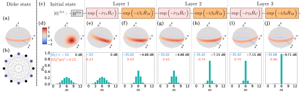
Figure 1: Metrologically useful squeezing generated by a depth-three QAOA for the MaxCut problem in a complete graph of 12 nodes. (a) Wigner quasi-probability distribution of the symmetric Dicke state $D^{12}_{6}$, an idealized example of a squeezed state and the target for our QAOA. (b) Fully connected unweighted graph with the nodes and edges colored according to one of the 924 possible maximum cut configurations. (c) Circuit representation of QAOA with alternating application of cost-function and mixer Hamiltonian. The Bloch spheres and histograms from (d) to (j) show the state after the corresponding gate in the optimized QAOA circuit with $(\gamma_{i},\beta_{i})$ given by $(0.199,0.127)$, $(0.306,0.087)$, and $(4.592,1.518)$ for $i=1$, $2$, and $3$, respectively. Negativity in the Wigner distribution indicates that the states are non-Gaussian Gross (2007). The squeezing (in black), energy expectation $\langle\hat{H}_{C}\rangle$ (in blue), and overlap probability density $|\langle D_{6}^{12}|\psi\rangle|^{2}$ with the target Dicke state (in orange) are shown inside each histograms.

Squeezing and quantum combinatorial optimization. Squeezed states are entangled states with a reduced variance of one observable at the cost of an increased variance in non-commuting observables. A large body of experimental work exists addressing the generation of squeezing in various platforms  Esteve et al. (2008); Purdy et al. (2013); Strobel et al. (2014); Muessel et al. (2015); Xu et al. (2022); Marciniak et al. (2022). Squeezing can also detect multipartite entanglement among qubits  Sørensen et al. (2001); Korbicz et al. (2005, 2006); Gühne and Tóth (2009); Tóth (2007).

In our setting, we are interested in squeezing within an ensemble of $n$ qubits (whose symmetric subspace can be seen as a qudit with length $\ell=\frac{n}{2}$). Consider a coherent state, such as the collective superposition $\ket{+}^{\otimes n}$, where $\ket{+}=(\ket{0}+\ket{1})/\sqrt{2}$. This state has a variance of $\sigma^{2}_{\text{css}}=\frac{n}{4}$, commonly called the shot-noise, in the collective observable $\hat{L}_{\textrm{z}}=\frac{1}{2}\sum_{i=1}^{n}\hat{Z}_{i}$. By evolving $\ket{+}^{\otimes n}$, e.g., under the non-linear one-axis-twisting (OAT) operator $\hat{L}_{\textrm{z}}^{2}=\frac{1}{4}(n+\sum_{i\neq j}\hat{Z}_{i}\hat{Z}_{j})$, the state is stretched over the collective Bloch sphere. The direction with reduced variance can be transferred to the $z$ coordinate by rotating the state around the $x$-axis with $\hat{L}_{x}=\frac{1}{2}\sum_{i=1}^{n}\hat{X}_{i}$ Kitagawa and Ueda (1993); Wang et al. (2001); Strobel et al. (2014). The resulting $n$ particle state is called number squeezed along $z$ when the observed variance is below $\sigma^{2}_{\text{css}}$, i.e., if the squeezing parameter

$$\mathcal{S}~{}[{\rm dB}]=10\log_{10}\left(\frac{\text{Var}(\hat{L}_{\textrm{z}})}{\sigma^{2}_{\text{css}}}\right)$$ (2)

is negative Kitagawa and Ueda (1993); Ma et al. (2011).

In a quantum circuit representation, it becomes apparent that these steps coincide with a single-layer QAOA sequence, see Fig. 1(c): (i) The application of Hadamard gates to $\ket{0}^{\otimes n}$ initialize the system in $\ket{+}^{\otimes n}$, the ground state of the mixer Hamiltonian $\hat{H}_{M}$. (ii) The evolution under the OAT operator corresponds to applying the unitary $\exp(-i\gamma_{1}\hat{H}_{C})$ with the cost function $\hat{H}_{C}\propto\hat{L}_{\textrm{z}}^{2}$. On the qubit level, this corresponds to controlled-z gates generated by $\hat{Z}_{i}\hat{Z}_{j}$ between all qubits $i$ and $j$. (iii) The rotation around the $x$-axis to reveal the squeezing corresponds to the unitary $\exp(-i\beta_{1}\hat{H}_{M})$, i.e., an application of the mixer.

The above cost function $\hat{H}_{C}\propto\hat{L}_{\textrm{z}}^{2}$ is a special instance of the MaxCut problem. MaxCut aims at bipartitioning the set of nodes $V$ in a graph $G(V,E)$ such that the sum of the weights $\omega_{i,j}$ of the edges $(i,j)\in E$ traversed by the cut is maximum, i.e.

$$\max_{z\in\{-1,1\}^{n}}\frac{1}{2}\sum_{(i,j)\in E}\omega_{i,j}(1-z_{i}z_{j}).$$ (3)

Consider the problem instance with $\omega_{i,j}=1,\forall(i,j)$, i.e., an unweighted fully connected graph labelled $\mathcal{G}_{n}$, see Fig. 1(b). Dividing $V$ into two sets of size as equal as possible creates a maximum cut. For even $n$, the set of all maximum cuts corresponds to the symmetric Dicke state Dicke (1954)

$$D_{k}^{n}={\binom{n}{k}}^{-1/2}\sum_{i}P_{i}\left(\ket{1}^{\otimes k}\otimes\ket{0}^{\otimes(n-k)}\right)\,,$$ (4)

with $k=\frac{n}{2}$. Here, $P_{i}(\cdot)$ denotes a permutation of all states with $k$ particles in $\ket{1}$ and $n-k$ particles in $\ket{0}$. For odd $n$, the set of all maximum cuts corresponds to $(D^{n}_{\lfloor n/2\rfloor}+D^{n}_{\lceil n/2\rceil})/\sqrt{2}$. These states are maximally squeezed along $z$ and are the most useful for metrological applications Pezzè et al. (2018). The QAOA cost function Hamiltonian to minimize in this problem is $\hat{H}_{C}=\frac{1}{2}\sum_{i<j}(\hat{Z}_{i}\hat{Z}_{j}-1)=\hat{L}_{z}^{2}-\frac{n^{2}}{4}\mathbb{I}$. Therefore, QAOA tasked to find the maximum cut of a fully connected unweighted graph will maximize the squeezing. This relation thus translates analog metrological protocols Strobel et al. (2014) to a digital quantum processor. In addition, by formulating the constraints that an arbitrary Dicke state $D_{k}^{n}$ imposes on the spins as a QUBO, we can generate $D_{k}^{n}$ for arbitrary $k$ Not .

QAOA as generator of squeezing. To illustrate this connection between QAOA and squeezing, we numerically simulate a system with $n=12$ qubits and follow the usual QAOA protocol, using $\hat{H}_{C}=\hat{L}_{z}^{2}-\frac{n^{2}}{4}\mathbb{I}$, $\hat{H}_{M}=-2\hat{L}_{x}$, and $p=3$ Not . We depict the generated collective qudit state using the Wigner quasi-probability distribution as well as the probability distribution over the spin eigenvalues $\{m=\langle\hat{L}_{z}\rangle+\frac{n}{2}\}$ at each step, see Fig. 1(d)-(j). Each application of $\hat{H}_{C}$ stretches the Wigner distribution making it resemble an ellipse with the major axis tilted with respect to the equatorial plane of the qudit Bloch sphere. As $[\hat{H}_{C},\hat{L}_{z}]=0$, this operation does not alter the distribution of $\langle\hat{L}_{z}\rangle$. Next, the mixer operator rotates the Wigner distribution back towards the equator, thereby transferring the squeezing to the operator $\hat{L}_{z}$. After three layers, the final state has an overlap with the symmetric Dicke state of $96\%$ and the squeezing number reaches $\mathcal{S}=-9.71~{}{\rm dB}$. Crucially, noiseless QAOA with less layers produces less squeezing, e.g., see depth-one QAOA Not .

The squeezing in collective spin observables can further be related to entanglement. We employ three different criteria Not : (E1) If $\frac{n}{4}>\langle\hat{L}_{\textrm{z}}^{2}\rangle$, the state violates a bound on separable states Tóth (2007). Any squeezed state ($\text{Var}(\hat{L}_{\textrm{z}})<\frac{n}{4}$) at the equator ($\langle\hat{L}_{\textrm{z}}\rangle=0$) is witnessed as entangled by this criterion. Here, $\langle\hat{L}_{\textrm{z}}^{2}\rangle=0.32<\frac{n}{4}=3$, which is close to the minimal value of $0$ achieved by the Dicke state. (E2) If the quantum Fisher information for a pure state $\psi$, $F_{Q}[\psi,\mathcal{O}]=4\text{Var}(\mathcal{O})$, is larger than $(sk^{2}+r^{2})$, where $s=\lfloor n/k\rfloor$ denotes the integer division of $n$ by $k$, and $r$ is the remainder, at least $(k+1)$ particles are entangled Hyllus et al. (2012); Tóth (2012). Here, $F_{Q}[\psi,\hat{L}_{\textrm{y}}]=84.48$ and the final state has multipartite entanglement between at least $9$ out of $12$ particles. (E3) Specifically for Gaussian states, one can approximately estimate the number of entangled particles $k$ assuming the identity $F_{Q}/n\simeq\sigma^{2}_{\mathrm{css}}/\text{Var}(\hat{L}_{\textrm{z}})$ Strobel et al. (2014); Not , which here yields $k=11$. We will use this estimate below in the hardware results where direct access to $F_{Q}$ is not possible. With $k+1$-partite entangled states the variance of a phase $\theta$ measured $m$ times satisfies $\Delta^{2}\theta\geq 1/(mkn)$ Tóth (2012). QAOA-generated Dicke states take more time to prepare than coherent states but have more entanglement. Even for the disadvantageous geometry of a linear chain, where entanglement needs to be linearly transported, and very moderate values of $k=2$, one can estimate the QAOA-generated states in current superconducting qubits to achieve a better $\Delta^{2}\theta$ in less time than coherent states for as many as 60 qubits, and this number rises exponentially with improved $k$. For hardware with slow repetition rates that natively implement the OAT operator, such as Bose-condensed cold-atoms Strobel et al. (2014), it is always advantageous to use QAOA-generated states Not .

Warm-start with squeezed states. The QAOA circuit that generates squeezed states can be reused as a circuit to create initial states for QAOAs designed to tackle graphs obtained from perturbations of the fully-connect unweighted graph. Such states lower the number of optimization parameters needed, making it simpler for the classical optimizer to handle Not .

QAOA-tailored hardware benchmarks. The performance of quantum computing hardware is often measured by metrics such as randomized benchmarking Magesan et al. (2011, 2012); Córcoles et al. (2013) and quantum process tomograph O’Brien et al. (2004); Bialczak et al. (2010), which focus on gates acting on typically one to two qubits, while Quantum Volume (QV) is designed to measure the performance of a quantum computer as a whole Cross et al. (2019); Jurcevic et al. (2021); Pelofske et al. (2022). For certain applications, these are complemented by specifically designed benchmarks, e.g., for quantum chemistry Arute et al. (2020), generative modelling Benedetti et al. (2019); Dallaire-Demers and Killoran (2018), variational quantum factoring Karamlou et al. (2021), Fermi-Hubbard models Dallaire-Demers et al. (2020), and spin Hamiltonians Schmoll and Orús (2017).

It is of particular interest to identify such application-tailored benchmarks also for variational algorithms, as these employ highly structured circuits. This necessity is well illustrated by considering the QV: the circuit complexity of a $2^{n}$ QV system is equivalent to a $p=2$ QAOA running on $n$ linearly connected qubits Not . As this shows, QV fails to properly capture the dependency on $p$ as QAOA circuits on complete graphs are deeper than their width. As Ref. França and García-Patrón (2021) shows using entropic inequalities, if the circuit is too deep a classical computer can sample in polynomial time from a Gibbs state while achieving the same energy as the noisy quantum computer. That bound is based on the fidelity of layers of gates, which is, however, often overestimated when built from fidelities of gates benchmarked in isolation, e.g., due to cross-talk Weidenfeller et al. (2022).

Since the solution to the MaxCut problem on the fully connected unweighted graph $\mathcal{G}_{n}$ is known, we propose squeezing as a good hardware benchmark for QAOA to complement other performance metrics. From a hardware perspective, although $\mathcal{G}_{n}$ is a specific problem, its QAOA circuit is representative of the noise of an arbitrary fully-connected QUBO problem since the gates constituting a generic cost function $\exp(-i\gamma_{k}\hat{H}_{C})$ can be implemented with virtual Z-rotations and CNOT gates McKay et al. (2017). The duration of the QAOA pulse-schedule and the absolute amplitude of the pulses are thus independent of the variables $\Sigma$ in the QUBO, see Eq. (1), and the variational parameters $\boldsymbol{\gamma}$ and $\boldsymbol{\beta}$. Therefore, the pulse-schedule of the squeezing circuit will capture the same amount of noise, such as decoherence, unitary gate errors, and cross-talk, as the QAOA circuit for an arbitrary QUBO Not .

For our proposed benchmark, we first label the quantum numbers of $\hat{L}_{z}+\frac{n}{2}$ by $m\in\{0,1,...,2\ell\}$, which correspond to cuts of size $c(m)=m(n-m)$ on $\mathcal{G}_{n}$. We relate squeezing to a QAOA performance metric through the question: Given the squeezing $\mathcal{S}$ in the trial state, what is the probability $P_{\alpha}(n,\mathcal{S})$ of sampling a cut with size $c(m)$ greater than a given $\alpha$-fraction of the maximum cut size $c_{\text{max}}=n^{2}/4$? Here, $\alpha$ can be seen as an approximation ratio. By definition, cuts with $c(m)>\alpha c_{\text{max}}$ must satisfy $m_{-}(\alpha)<m<m_{+}(\alpha)$ for even $n$, where $m_{\pm}(\alpha)=\frac{n}{2}(1\pm\sqrt{1-\alpha})$. Under a QAOA trial state $\ket{\psi(\boldsymbol{\beta},\boldsymbol{\gamma})}$ with a distribution $p_{m}$ over $m$, see Fig. 2(a), the probability to sample cuts larger than $\alpha c_{\text{max}}$ is thus

$$P_{\alpha}(n)=\sum_{m=\lceil m_{-}(\alpha)\rceil}^{\lfloor m_{+}(\alpha)\rfloor}p_{m}.$$ (5)

We now make the simplifying assumption that the distribution $p_{m}$ is a Gaussian $\mathcal{N}(\frac{n}{2},\sigma)$ , where the standard deviation $\sigma$—the only free variable for fixed $n$—is, by definition, in one-to-one correspondence to the squeezing $\mathcal{S}=10\log_{10}(4\sigma^{2}/n)$. In summary, the benchmark (i) relates squeezing to the probability of sampling good solutions, a QAOA performance metric, (ii) captures the ability of QAOA to create entangled states, and (iii) is as susceptible to hardware noise as other fully connected QAOA circuits.

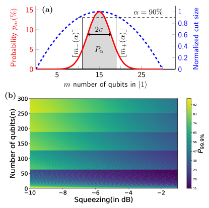
Figure 2: Benchmarking QAOA with squeezing. (a) Probability distribution ($p_{m}$, red solid line) and normalized cut size ($c_{m}/c_{max}$, blue dashed line) simultaneously plotted against $m=\langle\hat{L}_{\textrm{z}}\rangle+\frac{n}{2}$ for $n=30$. States with normalized cut-size more than $\alpha$ lie in $m\in[\lceil m_{-}(\alpha)\rceil,\lfloor m_{+}(\alpha)\rfloor]$. These yield the shaded area under the probability $p_{m}$, which is the figure of merit $P_{\alpha}$ defined in Eq. (5). (b) $P_{\alpha}$ showing how the probability of sampling high value cuts changes with the squeezing $\mathcal{S}$ and the number of qubits $n$, calculated using trial Gaussian distributions.

We illustrate the benchmark by numerically computing $P_{\alpha}(n,\mathcal{S})$ as a function of $n$ and the squeezing $\mathcal{S}$ in the Gaussian distribution $p_{m}(\mathcal{S})$. Since the ground state of $\mathcal{G}_{n}$ is highly degenerate, we select a high value of $\alpha$, e.g., $99.9\%$. At fixed $n$, an increased squeezing (more negative) increases $P_{\alpha}$, see Fig. 2(b), as cuts with a larger size receive more weight. In addition, $P_{\alpha}$ has discontinuous jumps at $n_{\text{dis.}}$, where $z=\lfloor\frac{n_{\text{dis.}}}{2}\sqrt{1-\alpha}\rfloor\in\mathbb{Z}^{+}$ Not . In between discontinuities, $P_{\alpha}$ diminishes with increasing $n$ because $\sigma$ increases $\propto\sqrt{n}$ for fixed $\mathcal{S}$, which reduces the weight attributed to high value cuts.

Benchmarking superconducting qubits. We now evaluate the benchmark on gate-based superconducting transmon qubits Krantz et al. (2019).

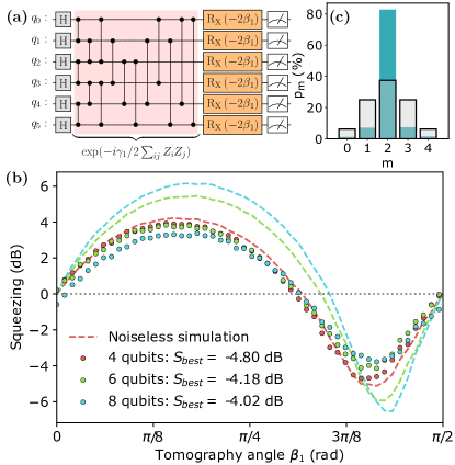
Figure 3: Squeezed states generated on superconducting qubits. (a) A quantum circuit implementing a single QAOA-layer for the MaxCut problem on a six-qubit system, producing a state with a reduced variance along the $z$-axis. (b) Squeezing measured with the quantum circuit in (a). The dashed lines show a noiseless Qasm simulation. (c) The $p_{m}$ distribution of the four-qubit state with $-5.96~{}{\rm dB}$ squeezing generated by a depth-two QAOA with optimal parameters $\gamma_{1}=0.918$, $\gamma_{2}=-0.257$, $\beta_{1}=-0.711$, and $\beta_{2}=-2.175$. The gray histogram shows the state $(H\ket{0})^{\otimes n}$.

We measure the squeezing on the IBM Quantum system ibmq_mumbai using Qiskit Anis et al. (2021) for four, six, and eight qubits Not . Since the chosen qubits have a linear connectivity, we use a line swap strategy Jin et al. (2021); Weidenfeller et al. (2022) to create the all-to-all qubit connectivity required by the squeezing circuit, shown in Fig. 3(a) for $p=1$. This circuit is then transpiled to the cross-resonance-based hardware Sheldon et al. (2016); Sundaresan et al. (2020) employing a pulse-efficient strategy instead of a CNOT decomposition Earnest et al. (2021) using Qiskit Pulse Alexander et al. (2020). The optimal value of the variational parameter $\gamma$ is found with a noiseless simulation for each $n$. We use readout error mitigation Bravyi et al. (2021); Barron and Wood (2020), which on average improves the best measured squeezing by $-0.7\pm 0.1~{}{\rm dB}$ averaged over all three $n\in\{4,6,8\}$. At depth one, a sweep of the tomography angle $\beta_{1}$ reveals a squeezing of $-4.80$, $-4.18$, and $-4.02~{}{\rm dB}$ whereas noiseless simulations reach $-5.14$, $-5.90$, and $-6.56~{}{\rm dB}$ for $n=4,6$, and $8$, respectively. These metrological gains are comparable to prior works in trapped ions Sackett et al. (2000); Meyer et al. (2001); Leibfried et al. (2003, 2004, 2005); Monz et al. (2011). Given the measured squeezing, we compute a $P_{99.9\%}(n,\mathcal{S})$ of $61.5\%$, $49.1\%$, and $42.6\%$, respectively. Furthermore, we run a depth-two QAOA on the fully connected four-qubit graph to create a state with a $-5.96~{}{\rm dB}$ squeezing, see Fig. 3(c), which results in $P_{99.9\%}(4,-5.96)=68.2\%$. These results indicate that the potential to generate squeezing in a four qubit system is limited by the variational form at depth one. By contrast, in systems with six and eight qubits, the squeezing generated in practice is limited by the large number of CNOT gates at depth one (40 and 77, respectively). The criterion (E1) witnesses the generated states in both simulation and hardware as entangled, see Fig. 4(a). In noiseless simulation of a depth-one QAOA of system sizes $n=4,6,8$, criterion (E2) witnesses at least $4,4,5$ qubit entanglement, respectively. In the noisy hardware implementation, estimate (E3) suggests these numbers to still reach $4,3,3$, respectively.

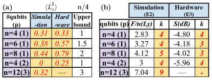
Figure 4: Entanglement from squeezing and quantum Fisher information. (a) The values of $\langle\hat{L}_{z}^{2}\rangle$ (E1) obtained in simulation and hardware are close to 0 indicating that the states are in the vicinity of entangled Dicke states. (b) Number of entangled particles $k$ calculated from $F_{Q}[\hat{L}_{y}]$ (E2) in simulation, and estimated for hardware using (E3).

Conclusion. In summary, the generation of squeezed states that are useful for metrology can be cast as a MaxCut problem, which in turn can be addressed with variational algorithms. The procedure that we illustrated in the creation of a 12 qubit Dicke state can be implemented on universal quantum computing platforms, such as superconducting qubits or trapped ions, as well as on special purpose machines such as BECs trapped in optical tweezers Strobel et al. (2014). Interestingly, an enhancement of squeezing within the multilayer QAOA protocol is not equivalent to simply applying the $\hat{L}_{z}^{2}$ operator for a longer period, as the mixer Hamiltonian periodically intervenes Not . Thus, our results show how variational algorithms may generalize existing protocols and provide systematic guidance for the creation of highly squeezed states for metrology. By contrast to, e.g., Ref Marciniak et al. (2022); Kaubruegger et al. (2019); Koczor et al. (2020); Meyer et al. (2021) which uses variational quantum algorithms with a hardware native ansatz to enhance phase sensitivity, the QAOA approach to create squeezing encapsulates the structure of the target state in the variational form which may reduce the number of parameters to optimize. In a similar vein, we foresee that custom states beyond Dicke states may be generated by QAOA if they can be cast as solutions of a combinatorial optimization problem. In addition, we suggested squeezing as a QAOA specific hardware benchmark. This benchmark is both portable across hardware platforms and captures hardware-specific properties such as limited qubit connectivity and cross-talk.

Acknowledgements. FJ and DJE are thankful to the organisers of the Qiskit Unconference in Finland and fruitful discussions with Arianne Meijer as well as Matteo Paris that started this work. The authors acknowledge use of the IBM Quantum devices for this work. GCS, FJ, and PH acknowledge support by the Bundesministerium für Wirtschaft und Energie through the project “EnerQuant” (Project- ID 03EI1025C). FJ acknowledges the DFG support through the Emmy-Noether grant (Project-ID 377616843). This work is supported by the DFG Collaborative Research Centre “SFB 1225 (ISOQUANT), by the Bundesministerium für Bildung und Forschung through the project “HFAK” (Project- ID 13N15632). PH acknowledges support by the ERC Starting Grant StrEnQTh (project ID 804305), Provincia Autonoma di Trento, and by Q@TN, the joint lab between University of Trento, FBK-Fondazione Bruno Kessler, INFN-National Institute for Nuclear Physics and CNR-National Research Council.

Supplemental Material: Squeezing and quantum approximate optimization In this Supplemental Material, we (i) discuss the details of the optimization method used to obtain the parameters $\{\boldsymbol{\gamma},\boldsymbol{\beta}\}$, (ii) describe why squeezed states are entangled, (iii) define and connect multipartite entanglement to quantum Fisher information and squeezing, (iv) discuss the practical advantages of using QAOA for metrology in different hardware architectures, (v) argue why squeezing can be a better benchmark than quantum volume in QAOA, (vi) explain the discontinuities observed in the benchmark in Fig.2(b), (vii) give details of the ibmq_mumbai, (viii) discuss the advantages of using multiple-layers of QAOA, (ix) explain why increasing the duration of $\hat{H}_{C}$ is not helpful compared to the alternating layers in QAOA, (x) discuss the creation of arbitrary Dicke states, and (xi) show how to initialize QAOA with squeezed states to lower the number of optimization parameter.

I Optimization method

The 12 qubit example in the main text is run with the Qiskit QAOA Runtime program Weidenfeller et al. (2022). To optimize the $\{\boldsymbol{\gamma},\boldsymbol{\beta}\}$ we use the simultaneous perturbation stochastic approximation (SPSA) algorithm Spall (1998) which simultaneously optimizes multiple parameters and can handle noisy environments. We do not initialize the optimizer with values for the learning rate and a perturbation. Instead, we let SPSA calibrate itself in the first 25 iterations. To obtain good solutions we allow SPSA a maximum of $500$ iterations and gather a total of $2^{15}$ shots per iteration.

II Entanglement from squeezing

Measurements of collective spin observables can reveal entanglement. In particular, separable states satisfy Tóth (2007)

$$\langle\hat{L}_{x}^{2}\rangle+\langle\hat{L}_{y}^{2}\rangle\leq\frac{n}{2}\bigg{(}\frac{n}{2}+\frac{1}{2}\bigg{)}\Longleftrightarrow\frac{n}{4}\leq\langle\hat{L}_{\textrm{z}}^{2}\rangle=\text{Var}(\hat{L}_{\textrm{z}})\,.$$ (S6)

The second implication is reached using the identity $\langle\hat{L}^{2}\rangle=\langle\hat{L}_{x}^{2}\rangle+\langle\hat{L}_{y}^{2}\rangle+\langle\hat{L}_{z}^{2}\rangle=\frac{n}{2}(\frac{n}{2}+1)$, and $\langle\hat{L}_{\textrm{z}}\rangle=0$ for our target states. Any squeezed state defined through Eq. (2) violates the relation above and is thus entangled. Moreover, $\langle\hat{L}_{x}^{2}\rangle+\langle\hat{L}_{y}^{2}\rangle$ reaches the maximum $\frac{n}{2}(\frac{n}{2}+1)$ in the Dicke state Tóth (2007), which is the same as having $\text{Var}(\hat{L}_{\textrm{z}})=0$. In Fig. 4(a), we show how the obtained values of $\langle\hat{L}_{\textrm{z}}^{2}\rangle$ are close to the minimum limit $0$, revealing the existence of significant entanglement.

III Multipartite entanglement, quantum Fisher information, and squeezing

A pure state of $n$-qubits, written as a product $\ket{\psi}=\otimes_{j=1}^{M}\ket{\psi_{j}}$, is $k$-partite entangled when at least one state $\ket{\psi_{j}}$ contains non-factorizable $k$-qubits Hyllus et al. (2012); Apellaniz et al. (2015). This definition is the same as the entanglement depth  Lücke et al. (2014), see Fig. S5(c). A sufficient condition for $(k+1)$-partite entanglement stems from the quantum Fisher information $F_{Q}$: a state reaching $F_{Q}[\rho_{n},\mathcal{O}]>(sk^{2}+r^{2})$—where $s=\lfloor n/k\rfloor$ denotes the integer division of $n$ by $k$, and $r$ is the remainder—is at least $(k+1)$-partite entangled Hyllus et al. (2012); Tóth (2012).

While $F_{Q}$ is becoming a useful witness for entanglement in quantum many-body systems Hauke et al. (2016); Smith et al. (2016); Wang et al. (2014); Yin et al. (2019); Mathew et al. (2020); Laurell et al. (2021), its origin is as a key figure of merit in quantum metrology, where $F_{Q}$ quantifies the distinguishability of a state $\rho$ from $\rho^{\prime}=e^{-i\theta\mathcal{O}}\rho e^{i\theta\mathcal{O}}$, generated by the Hermitian operator $\mathcal{O}$ with infinitesimal $\theta$. Thus, a large $F_{Q}$ implies a high measurement precision for estimating the value of $\theta$ Braunstein and Caves (1994); Pezze and Smerzi (2014). For pure states $\psi$, the quantum Fisher information becomes simply $F_{Q}[\psi,\mathcal{O}]=4\textrm{Var}(\mathcal{O})_{\psi}$ Tóth and Apellaniz (2014), whereas for mixed states it provides a lower bound on the variance.

The target state of the QAOA for MaxCut on $\mathcal{G}_{n}$, the Dicke state, is invariant under a unitary evolution generated by $\hat{L}_{\textrm{z}}$ but is highly sensitive to rotations around the $x$- or $y$-axes of the collective Bloch sphere Strobel et al. (2014). Thus, to obtain a large $F_{Q}$, it is advantageous to choose $\mathcal{O}=\hat{L}_{x}$ or—even more so—$\mathcal{O}=\hat{L}_{y}$. We report $F_{Q}$ in Fig. S5(b) for both $\mathcal{O}=\hat{L}_{x},\hat{L}_{y}$ and the resulting $k$-partite entanglement witnessed by it for the ideal simulations. In this ideal scenario of noiseless numerical simulations, the large values of $F_{Q}[\psi,\hat{L}_{x,y}]$ are directly related to the anti-squeezing of the final state along the equator of Bloch sphere.

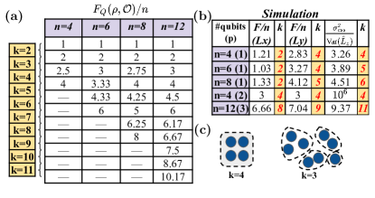
Figure S5: Multipartite entanglement from quantum Fisher information and number squeezing. (a) $F_{Q}$ witnessing $k$-partite entanglement for different $n$, (b) In the simulations, $F_{Q}$ obtained with $\hat{L}_{y}$ is larger than $\hat{L}_{x}$. The numbers of entangled particles ($k$) estimated from squeezing ($\sigma^{2}_{\mathrm{css}}/\text{Var}(\hat{L}_{\textrm{z}})=10^{-\mathcal{S}/10})$ are close to the numbers obtained from $F_{Q}[\hat{L}_{y}]$ for most cases. In a proper Dicke state as obtained with $n=4(p=2)$, the $\text{Var}(\hat{L}_{\textrm{z}})$ becomes extremely small, leading to the very large value of $\sigma^{2}_{\mathrm{css}}/\text{Var}(\hat{L}_{\textrm{z}})$ seen in the fourth row. (c) Illustrative examples of $k$-partite entanglement as entanglement depth.

In the hardware, where the system is no longer in a pure state, it is considerably more challenging to directly access $F_{Q}$ Hauke et al. (2016); Costa de Almeida and Hauke (2021). However, for Gaussian states, one can nevertheless use the empirical relation Strobel et al. (2014)

$$F_{Q}/n[\hat{L}_{y}]\simeq\sigma^{2}_{\mathrm{css}}/\text{Var}(\hat{L}_{\textrm{z}})=10^{-\mathcal{S}/10}$$ (S7)

between $F_{Q}$ and squeezing. For the simulation, the estimated $k$ using this relation is close to the exact estimation from $F_{Q}$ in most of cases, see Fig. S5(b), except for the depth-three QAOA, where the states are no longer Gaussian Gross (2007). Assuming that the above relation holds for depth-one QAOA, where the states are expected to be Gaussian, we obtain the estimates for $k$-partite entanglement in the hardware implementation reported in Fig. 4(b) of the main-text.

IV Metrology

In this section, we study the time taken to measure a phase $\theta$ with the CSS verus QAOA-generated Dicke states within different hardware architectures (but without an attempt at comparing the different architectures to each other, which often have different aims and boundary conditions that are difficult to compare on an even footing). The coherent state is easily prepared by a single rotation around the $y$-axis. It has no entanglement, and $m$ measurements of the phase $\theta$ have a variance bound by $\Delta^{2}\theta\geq 1/(mN)$. By contrast, a QAOA prepared state with $F_{Q}$ above the $k+1$-partite entangled limit takes more time to prepare than the CSS, but it requires a smaller number of measurements to reach the same variance since $\Delta^{2}\theta\geq 1/(mkN)$ is lowered by a factor of $1/k$.

One may then wonder whether, in a practical application, the improved precision can offset the larger preparation time. Crucially, the optimization cost of QAOA can be ignored in these considerations since the optimal $\boldsymbol{\gamma}$ and $\boldsymbol{\beta}$ parameters are reusable across different measurements and experiments. We therefore compute the duration of a single measurement repetition $t_{\text{repet.}}$, which is the sum of the duration of the gates in the circuit to prepare the state $t_{\text{gates}}$ and the readout time including the reset of the measurement apparatus $t_{\text{rr}}$, i.e., $t_{\text{repet.}}=t_{\text{gates}}+t_{\text{rr}}$. The gate duration for the coherent spin state $t_{\text{gate}}^{\text{CSS}}$ is the duration of a single-qubit gate, while the QAOA protocol requires two-qubit gates, whose number can depend on the available universal gate set and the hardware connectivity.

The QAOA-generated states are advantageous when the time $t^{\text{QAOA}}=t_{\text{repet.}}^{\text{QAOA}}m_{\text{QAOA}}$ to achieve a certain precision is smaller than the time $t^{\text{CSS}}=t_{\text{repet.}}^{\text{CSS}}m_{\text{CSS}}$ to achieve the same precision with coherent states. If the QAOA-prepared state achieves $F_{Q}=kN$, we have for equal precision $m_{\text{QAOA}}k=m_{\text{CSS}}$, i.e., the QAOA-prepared states are advantageous if

$$t_{\text{gates}}^{\text{QAOA}}+t_{\text{rr}}<k\left(t_{\text{gates}}^{\text{CSS}}+t_{\text{rr}}\right).$$ (S8)

Superconducting qubits:

The duration of a QAOA layer is impacted by the qubit connectivity. Each QAOA layer on $N$ linearly connected superconducting qubits requires $3(N-2)$ layers of simultaneously executable CNOT gates which includes SWAP gates Weidenfeller et al. (2022). Under the assumption that QAOA can create $k+1$-partite entanglement in $p=\log_{2}(k)$ layers Farhi et al. (2020), the duration $t_{\text{gates}}^{\text{QAOA}}=3(N-2)\log_{2}(k)t_{\text{cx}}$ with $t_{\text{cx}}$ the duration of a CNOT gate. Here, we neglected the duration of single-qubit gates. With $k=N$, Eq. (S8) yields

$$3(N-2)\log_{2}(N)t_{\text{cx}}+t_{\text{rr}}\lesssim Nt_{\text{rr}}$$ (S9)

which, for large $N$ and the durations in Tab. 1, amounts to

$$N\lesssim 2^{t_{\text{rr}}/(3t_{\text{cx}})}=2^{1000/3}.$$ (S10)

Although the linear layout of the hardware poses a limit onto when QAOA-generated states remain useful, this limit is extremely high. Assuming noisy hardware achieves only a finite $k$, one has

$$(N-2)\log_{2}N<(k-1)t_{\text{rr}}/(3t_{\text{cx}})\,.$$ (S11)

For $k=2$, e.g., the QAOA-generated states would remain advantageous up to about 60 qubits arranged in a linear chain, which lies at the size limit of current hardware. These numbers are conservative estimates that can be significantly increased by improved noise resilience and higher hardware connectivity.

Trapped-ion qubits:

Large multipartite entangled states of trapped-ions can be generated by a single application of the Mølmer–Sørensen gate (MS) Sørensen and Mølmer (1999); Sackett et al. (2000) where interaction strength among all qubit pairs is equal Lanyon et al. (2011). Therefore, if we neglect the duration of single-qubit gates, $t_{\text{gates}}^{\text{QAOA}}$ only depends on the number of QAOA layers $p=\log_{2}(k)$, and $t_{\text{gates}}^{\text{QAOA}}=\log_{2}(k)t_{ms}$ with $t_{ms}$ being the duration of a MS gate. Following Tab. 1, QAOA-generated $k+1$-partite entangled states are therefore advantageous when

$$\log_{2}(k)t_{\textrm{ms}}\lesssim(k-1)t_{\textrm{rr}}\Rightarrow k^{\frac{1}{k-1}}\lesssim 2^{t_{\textrm{rr}}/t_{\textrm{rm}}}=2^{25}.$$ (S12)

Since $k^{1/{(k-1)}}$ is a decreasing function, QAOA generated states are always advantageous in trapped-ion setups.

Cold-atoms:

We now consider cold-atoms in Bose-Einstein condensates which can, e.g., manipulate states with of the order of 400 atoms Strobel et al. (2014). Following QAOA, we assume that $\log_{2}(k)$ layers of the one-axis-twisting Hamiltonian interleaved with $x$-rotations can generate $k+1$-partite entanglement. The squeezed state is thus created in a time $t_{\text{gates}}^{\text{QAOA}}=\log_{2}(k)t_{\text{OAT}}$. We neglect the duration of $x$ and $y$-rotations. Equation (S8) implies $\log_{2}(k)t_{\text{OAT}}<(k-1)t_{\text{rr}}$, showing that given a Bose-condensed atom cloud of fixed size it is always favorable to create spin squeezed states for metrology since $t_{\text{OAT}}\ll t_{\text{rr}}$, see Tab. 1.

Platform	Single-qubit	Entanglement	Readout & Reset $t_{\text{rr}}$
Transmons	$10$ ns Werninghaus et al. (2021)	$100$ ns Jurcevic et al. (2021)	$100~{}\mu$s Wack et al. (2021)
Trapped ions Pogorelov et al. (2021)	$15~{}\mu$s	$200~{}\mu$s	$300~{}\mu$s $+5$ ms Schindler et al. (2013)
Cold atoms (BEC)		$10$ ms Strobel et al. (2014)	$1$ s

Table 1: Duration of key operations presented as orders of magnitude only. The entangling operation for the transmons, trapped-ions and cold atoms is the two-qubit CNOT gate, the Mølmer–Sørensen gate, and the one axis twisting Hamiltonian, respectively.

V Quantum Volume and QAOA benchmarking

A processor with a Quantum Volume of $QV=2^{n}$ can reliably, as defined by the generation of heavy output bit-strings, execute circuits that apply $n$ layers of ${\rm SU}(4)$ gates on random permutations of $n$ qubits Cross et al. (2019). When transpiled to a line of $n$ qubits, QV circuits result in $n$ layers of ${\rm SU}(4)$ gates that have at most $\left\lfloor\frac{n}{2}\right\rfloor$ individual ${\rm SU}(4)$ gates simultaneously executed on the qubits Jurcevic et al. (2021). In between these ${\rm SU}(4)$ layers, there are at most $\left\lfloor\frac{n}{2}\right\rfloor$ SWAP gates, see Fig. S6. Furthermore, each ${\rm SU}(4)$ and SWAP gate require at most and exactly three CNOT gates, respectively Vidal and Dawson (2004). Under these conditions, the total number of CNOT gates is at most

$$3n\left\lfloor\frac{n}{2}\right\rfloor+3(n-1)\left\lfloor\frac{n}{2}\right\rfloor\,,$$ (S13)

which approaches $3n^{2}$ as $n$ becomes large. By comparison, the cost operator of QAOA circuits of complete graphs transpiled to a line requires exactly $\frac{3}{2}n(n-1)-n+1$ CNOT gates, approaching $3n^{2}/2$ for large $n$. This suggests that a $2^{n}$ Quantum Volume is a good performance indicator for a depth $p=2$ QAOA on $n$ qubits. Importantly, this comparison is only possible as long as the QAOA circuit is executed using the same error mitigation and transpilation methods as those employed to measure QV Pelofske et al. (2022). However, QV fails to capture the depth dependency $p$ of QAOA. The benchmark that we develop overcomes this limitation as the QAOA depth should be chosen such that the measured squeezing is maximum. This also provides the maximum $p$ for which it makes sense to run QAOA on the benchmarked noisy hardware.

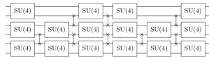
Figure S6: Example of a six-qubit quantum volume circuit as presented in Ref. Jurcevic et al. (2021), which shows the layers of ${\rm SU}(4)$ and SWAP gates.

From a hardware perspective, the squeezing circuit, exemplified in Fig. S7(a), captures the complexity of the pulses that execute an arbitrary fully-connected QUBO. Indeed, the difference between the pulse schedules only amounts to phase changes, indicated by circular arrows in Fig. S7(c). The duration and magnitude of the cross-resonance pulses are identical, compare Fig. S7(b) and (c). Therefore, much like Quantum Volume, the hardware benchmark based on squeezing captures effects such as limited qubit connectivity, unitary gate errors, decoherence, and cross-talk. Furthermore, from a hardware perspective the squeezing circuit is also the hardest to implement since QUBOs that are not fully connected, i.e., $\exists~{}(i,j)~{}|~{}\Sigma_{i,j}=0$, require less pulses.

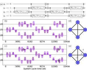
Figure S7: Cross-resonance pulse schedules of the squeezing circuit and an arbitrary QUBO. (a) Quantum circuit of a general four qubit fully connected cost operator $e^{-i\gamma\hat{H}_{C}}$ transpiled to qubits 0, 1, 3, and 5 of ibm_lagos. (b) Pulse schedule of the cost operator used to generate the symmetric Dicke state, i.e., $\omega_{i,j}=1~{}\forall i,j$. (c) Pulse schedule of a MaxCut instance with edge weights $\omega_{0,1}=\omega_{0,2}=\omega_{1,3}=-1$ and $\omega_{0,3}=\omega_{1,2}=\omega_{2,3}=1$. The circular arrows show where the phase shifts differ from the pulse schedule in (b). (d) and (e) MaxCut graph corresponding to the pulse schedule in (b) and (c), respectively. The duration of a single sample of the arbitrary waveform generators is ${\rm d}t=0.222~{}{\rm ns}$. The light and dark pulses show the in-phase and quadrature of each complex amplitude pulse applied to control channels U0, U5, and U8 of ibm_lagos.

VI Discontinuities in the QAOA hardware benchmark

According to Eq. (5), the states in the domain $(\lceil m_{-}\rceil,\lfloor m_{+}\rfloor)$ are included in $P_{\alpha}$, where $m_{\pm}(n,\alpha)=\frac{n}{2}\pm\frac{n}{2}\sqrt{1-\alpha}$. Since $\lfloor m_{+}\rfloor$ and $\lceil m_{-}\rceil$ must both be integers, the span of the domain $\lfloor m_{+}\rfloor-\lceil m_{-}\rceil$ remains constant over a large $n$ range and changes abruptly when $\lfloor\frac{n}{2}\sqrt{1-\alpha}\rfloor\in\mathbb{Z}$ changes value. We denote the values of $n$ at which such changes occur as $n_{\text{dis.}}$, which correspond to the discrete jumps along the $n$-axis in Fig. 2(b) of the main text. For $\alpha=99.9\%$ and $n$ even, we obtain discontinuities in $P_{99.9\%}$ at $n_{\text{dis.}}=64,128,190,254$.

VII Hardware details

The superconducting qubit data is gathered on the ibmq_mumbai system which has 27 fixed-frequency qubits connected through resonators; its coupling map is shown in Fig. S8. We chose a set of qubits that form a line with the smallest possible CNOT gate error. Each circuit is measured with 4000 shots. The properties of the device such as $T_{1}$ times and CNOT gate error are shown in Tab. 2.

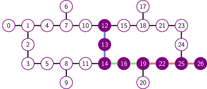
Figure S8: Coupling map of ibmq_mumbai with the qubits used shown in violet. The four, six, and eight qubit data were measured on the linearly connected qubits $\{19,22,25,26\}$, $\{14,16,19,22,25,26\}$, and $\{12,13,14,16,19,22,25,26\}$, respectively, chosen based on the CNOT gate fidelity.

CNOT gate
Qubit pair	error (%)	duration (ns)		Qubit	$\quad T_{1}~{}(\mu{\rm s})$
(12, 13)	0.77	548		12	166
(13, 14)	1.26	320		13	137
(14, 16)	1.04	348		14	174
(16, 19)	0.77	747		16	118
(19, 22)	0.66	363		19	227
(22, 25)	0.58	484		22	122
(25, 26)	0.50	348		25	194
	0.80$\pm$0.27	451$\pm$155		26	103

Table 2: Properties of the relevant CNOT gates as reported by ibmq_mumbai on the date of the circuit execution. The average $T_{1}$ of the selected qubits is $155\pm 43~{}\mu{\rm s}$.

VIII Increasing the duration of $\hat{H}_{C}$

Squeezing is generated by $\hat{L}_{\textrm{z}}^{2}$ Strobel et al. (2014), which suggests that simply applying $\hat{H}_{C}\propto\hat{L}_{\textrm{z}}^{2}$ for a longer duration, corresponding to a larger coefficient $\gamma$ in the QAOA, may transform the coherent state to a squeezed state, after which we can use the mixer $\hat{H}_{M}$ to reveal the squeezing along $\hat{L}_{\textrm{z}}$ as in the main text. In this way, one layer of QAOA would suffice to create any squeezing which would also require fewer CNOT gates than when $p>1$. To test this hypothesis, we run depth-one QAOA using $\gamma=\gamma_{1}+\gamma_{2}+\gamma_{3}$ where the $\gamma_{i}$ are taken from Fig. 1 in the main text, as they contain the source of “total” squeezing. The result is a fragmented Wigner distribution on the Bloch sphere without observable squeezing in any direction, see Fig. S9(a). Furthermore, no squeezing is detected along $z$ for any value of the tomography angle $\beta$, see Fig. S9(b). This finding is in agreement with the known observation that over-squeezing can be detrimental for precision Strobel (2016), however, the states here do not wrap around points near poles because $\hat{L}_{\textrm{z}}^{2}$ and $\hat{L}_{x}$ are not applied simultaneously as in Ref. Strobel (2016).

IX Advantages of multi-layer QAOA

One may object to the arguments in the preceding Appendix VIII that the $\gamma$ we chose is sub-optimal. To address that, in Fig. S9(c), we numerically map the energy landscape of depth-one QAOA in the $\{\gamma,\beta\}$ plane. The results reveal a minimum energy of $\langle\hat{H}_{C}\rangle_{\mathrm{min}}=-35.47$ which corresponds to $|\langle D^{12}_{6}|\psi\rangle|^{2}=98.53\%$. These results are inferior to those we obtain from the depth-three QAOA, i.e., $\langle\hat{H}_{C}\rangle_{\mathrm{min}}=-35.68$ and $|\langle D^{12}_{6}|\psi\rangle|^{2}=99.08\%$. Alternating multiple layers of $\hat{H}_{C}$ and $\hat{H}_{M}$ is therefore advantageous over a single application of the one-axis-twisting operator.

To quantify the obtainable improvement as a function of the number of layers used, we can define a new performance metric $\Delta^{n}_{p}(\%)$, which compares the energy reduction over the initial ansatz obtained by $p$-layers of QAOA with the one achieved by the ideal target state. In the $n=12$ case, the initial coherent state and the target Dicke state have $\langle\hat{H}_{C}\rangle=-33$, and $-36$, respectively. Thus, a depth-one QAOA (corresponding to the usual squeezing protocol) can reach a maximum $\Delta^{12}_{1}=2.47/3$. In contrast, the depth-three QAOA can reach $\Delta^{12}_{3}=2.68/3$, as shown in Fig. 1. Thus, according to this metric a depth-three QAOA is $0.21/3=7\%$ better than a depth-one QAOA.

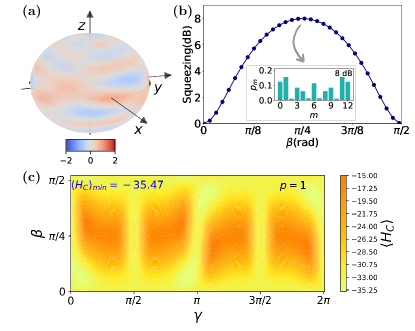
Figure S9: Illustration of the importance of alternating the cost-function and the mixer operator. (a) A fragmented Wigner distribution on the Bloch sphere is obtained when $\hat{H}_{C}$ is applied with $\gamma=\gamma_{1}+\gamma_{2}+\gamma_{3}$ from Fig. 1. (b) For the state in (a) no squeezing is observed at any $\beta$. The inset shows the probability distribution at $\beta=\pi/4$, corresponding to $\mathcal{S}=8~{}{\rm dB}$, i.e. over-squeezing. (c) The energy landscape of the depth-one QAOA reveals that the lowest energy it can reach is $-35.47$, which is inferior to $-35.68$ obtained in depth-three QAOA.

X Creating arbitrary Dicke states

In this section, we show how to create arbitrary Dicke states (Eq. 4) by minimizing a QUBO cost function with QAOA. Let $\ket{x_{n-1}...x_{0}}$ be a basis state in which qubit $i$ is in state $x_{i}\in\{0,1\}$. Each basis state in $D_{k}^{n}$ satisfies the equation $\sum_{i=0}^{n-1}x_{i}=k$, which is a constraint on the binary variables $x_{i}$. We express this constraint as the QUBO problem

$$\min_{x\in\{0,1\}^{n}}\left(k-\sum_{i=0}^{n-1}x_{i}\right)^{2}.$$ (S14)

The solution to this optimization problem is a superposition of all basis states with $k$ qubits in the excited state, i.e., $D_{k}^{n}$. We apply the change of variables $x_{i}=(z_{i}+1)/2$ to rewrite $(k-\sum_{i}x_{i})^{2}$ as

$$k^{2}-kn+\frac{n}{4}(n+1)+\left(\frac{n}{2}-k\right)\sum_{i=0}^{n-1}z_{i}+\frac{1}{2}\sum_{i<j}z_{i}z_{j}.$$ (S15)

After promoting each $z_{i}$ variable to a Pauli spin operator $\hat{Z}_{i}$, Eq. (S15) yields a cost Hamiltonian to minimize

$$\hat{H}_{C}=\left(\frac{n}{2}-k\right)\sum_{i=0}^{n-1}\hat{Z}_{i}+\frac{1}{2}\sum_{i<j}\hat{Z}_{i}\hat{Z}_{j}.$$ (S16)

When $k=n/2$, we recover the MaxCut problem on the symmetric graph. For $k\neq n/2$, we have an extra term $(n/2-k)\sum\hat{Z}_{i}$ that biases the total spin towards $\langle\hat{Z}\rangle=k$. The Hamiltonian in Eq. (S16) can therefore be used to generate the Dicke state $D_{k}^{n}$ with QAOA.

For n=12 qubits, we use the cost Hamiltonian in Eq. (S16) to simulate the generation of Dicke states with $k=1,2,3,4,5$. With three QAOA layers, we obtain fidelities in excess of 80%, see Fig. S10. The corresponding QAOA parameters $\boldsymbol{\gamma}$ and $\boldsymbol{\beta}$ are shown in Tab. 3.

Num. spin up $k$	$\gamma_{1}$	$\beta_{1}$	$\gamma_{2}$	$\beta_{2}$	$\gamma_{3}$	$\beta_{3}$
1	0.101	0.903	0.317	1.324	1.506	-0.155
2	0.093	1.106	0.427	1.409	1.457	-0.068
3	0.149	1.205	1.645	1.576	0.472	-0.076
4	0.111	1.220	0.441	1.690	1.028	0.062
5	0.231	1.340	1.643	1.500	1.774	0.004

Table 3: The parameters $(\gamma_{i},\beta_{i})$ of an optimized depth-three QAOA circuit to create $k=1,2,3,4,5$ Dicke states.

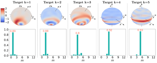
Figure S10: Metrologically useful arbitrary Dicke states generated by a depth-three QAOA by minimizing the cost Hamiltonian Eq. (S16). The top panels show the Wigner quasi-probability distribution on the Bloch spheres. The bottom panels show the corresponding histograms of the total spin operator $\langle\hat{Z}\rangle=m$. The orange numbers in each historgram show the overlap probability density $|\langle D_{k}^{12}|\psi\rangle|^{2}$ with the target Dicke states.

XI Warm-start with a Dicke state

In this section, we explore in how far the symmetric MaxCut problem that has a Dicke state as ground state can help solve also non-trivial asymmetric problems. We show how such squeezed states increase the likelihood to sample good cuts on random Erdős–Rényi graphs. Each edge $\omega_{i,j}$ of a graph is sampled from a Gaussian distribution $\mathcal{N}(\mu,\epsilon)$ and then rounded to one decimal place to increase the separation in the cut-values of the graph. We compare standard QAOA with $p$ layers to a QAOA with $p_{\text{s}}+p$ layers in which the first $p_{\text{s}}$ layers have fixed parameters to produce a squeezed state. Both methods, therefore, have $2p$ parameters that require optimization for each graph instance. For the second approach, in addition, $2p_{\text{s}}$ parameters are optimized once with the symmetric MaxCut problem as target and are reused for different problem instances. For each $n\in\{4,6,8,10,12\}$, we sample 100 graph instances from $\mathcal{N}(\mu,\epsilon)$ for which we chose $\mu=4$ and $\epsilon=0.5$ and optimize the cut-value for varying $p$. The resulting energy normalized to the minimum energy and averaged over the 100 graph realizations is used to compare both methods. To ensure that $p$ layers always produce a result that is at least as good as the one for $p-1$ layers, we bootstrap the optimization parameters. The initial guess of the parameters for layer $p$ are based on the optimized parameters of layer $p-1$, i.e., $(\beta_{1},\beta_{2},.....,\beta_{p},\gamma_{1},\gamma_{2},......,\gamma_{p})_{initial}=(\beta^{\rm{opt}}_{1},\beta^{\rm{opt}}_{2},.....,\beta^{\rm{opt}}_{p-1},0,\gamma^{\rm{opt}}_{1},\gamma^{\rm{opt}}_{2},......,\gamma^{\rm{opt}}_{p-1},0)$.

QAOA initialized with squeezed states, shown as orange circles and green stars in Fig. S12, significantly improves the average energy when compared to QAOA initialized from an equal superposition, shown as blue triangles in Fig. S12. We observe little improvement in solution quality with increasing $p$. We attribute this to the complexity of the optimization landscape which has many local minima, even at depth-one, due to the interference of the frequencies generated by the different edge weights, see Fig. S11. In the four qubits case, the energy for $p\geq 3$ layers of both methods is comparable. As the system size is increased, we observe a greater advantage for QAOA initialized with a squeezed state. These results indicate that, when solving a family of problems, it may be advantageous to initialize QAOA with a state that corresponds to the average problem even when such a problem is trivial to solve.

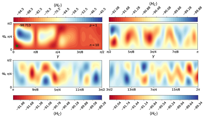
Figure S11: Complexity of the optimization landscape for a $n=10$ vertices graph with edge weights $[$3.1, 3.5, 3.9, 3.6, 4.6, 4.2, 4.8, 3.8, 4.1, 4.8, 5.0, 4.8, 4.0, 3.8, 3.2, 4.1, 4.2, 4.6, 4.3, 3.5, 3.9, 3.8, 3.2, 3.2, 4.7, 3.7, 4.1, 3.5, 4.1, 4.0, 4.2, 3.6, 4.4, 4.1, 3.5, 4.2, 3.7, 3.4, 4.4, 4.4, 3.6, 4.0, 4.3, 4.9, 4.1$]$ and QAOA depth $p=1$. Out of the full landscape, we show the first $0$ to $2\pi$ portion of the $\gamma$ landscape in four subplots $\gamma\in[0,\pi/2],[\pi/2,\pi],[\pi,3\pi/2],[3\pi/2,2\pi]$ with different color scales to increase the contrast between the local minima and maxima. This reveals a large number of local minima. The small improvement in solution quality with increasing $p$ can therefore be attributed to the many local minima, created from the interference of the frequencies generated by the different edge weights.

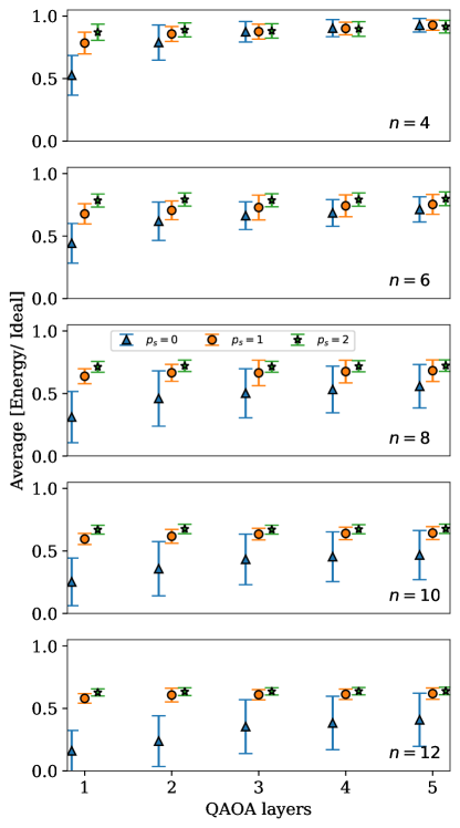
Figure S12: Advantage of QAOA initialized with squeezed states. The blue triangles show standard QAOA initialized from a coherent spin state. The orange circles and green stars show QAOA initialized with a spin-squeezed state created with $p_{s}=1$ and $2$ QAOA layers, respectively. The $x$-axis is the QAOA depth after the initial state and the y-axis is the energy normalized to the ideal value. The markers and error bars indicate the average and variance of 100 graph instances drawn from $\mathcal{N}(4,0.5)$ with different sizes $n=4$ (top) to $n=12$ (bottom). Squeezed initial states boost the average energy of the QAOA optimized state as shown by the orange and green markers having an energy that is closer to the ideal energy than the blue markers. The energy increases only modestly as $p$ increases due to the complexity of the optimization landscape.

References

- Farhi et al. (2014) Edward Farhi, Jeffrey Goldstone, and Sam Gutmann, “A quantum approximate optimization algorithm,” (2014), arXiv:1411.4028 .
- Torta et al. (2021) Pietro Torta, Glen B. Mbeng, Carlo Baldassi, Riccardo Zecchina, and Giuseppe E. Santoro, “Quantum approximate optimization algorithm applied to the binary perceptron,” arXiv:2112.10219 (2021).
- Headley et al. (2020) David Headley, Thorge Müller, Ana Martin, Enrique Solano, Mikel Sanz, and Frank K. Wilhelm, “Approximating the quantum approximate optimisation algorithm,” arXiv:2002.12215 (2020).
- Lucas (2014) Andrew Lucas, “Ising formulations of many NP problems,” Front. Phys. 2, 5 (2014).
- Liang et al. (2020) Daniel Liang, Li Li, and Stefan Leichenauer, “Investigating quantum approximate optimization algorithms under bang-bang protocols,” Phys. Rev. Research 2, 033402 (2020).
- Lee et al. (2021) Juneseo Lee, Alicia B. Magann, Herschel A. Rabitz, and Christian Arenz, “Progress toward favorable landscapes in quantum combinatorial optimization,” Phys. Rev. A 104, 032401 (2021).
- Streif and Leib (2019) Michael Streif and Martin Leib, “Comparison of QAOA with quantum and simulated annealing,” (2019), arXiv:1901.01903 .
- Wurtz and Love (2022) Jonathan Wurtz and Peter J. Love, “Counterdiabaticity and the quantum approximate optimization algorithm,” Quantum 6, 635 (2022).
- Pezzé and Smerzi (2009) Luca Pezzé and Augusto Smerzi, “Entanglement, nonlinear dynamics, and the Heisenberg limit,” Phys. Rev. Lett. 102, 100401 (2009).
- Pezzè et al. (2018) Luca Pezzè, Augusto Smerzi, Markus K. Oberthaler, Roman Schmied, and Philipp Treutlein, “Quantum metrology with nonclassical states of atomic ensembles,” Rev. Mod. Phys. 90, 035005 (2018).
- Degen et al. (2017) Christian L. Degen, Friedemann Reinhard, and Paola Cappellaro, “Quantum sensing,” Rev. Mod. Phys. 89, 035002 (2017).
- Gross et al. (2010) Christian Gross, Tilman Zibold, Euler Nicklas, Jerome Estève, and Markus K. Oberthaler, “Nonlinear atom interferometer surpasses classical precision limit,” Nature 464, 1165–1169 (2010).
- Sewell et al. (2012) Robert J. Sewell, Marco Koschorreck, Mario Napolitano, Brice Dubost, Naeimeh Behbood, and Morgan W. Mitchell, “Magnetic sensitivity beyond the projection noise limit by spin squeezing,” Phys. Rev. Lett. 109, 253605 (2012).
- Barsotti et al. (2018) Lisa Barsotti, Jan Harms, and Roman Schnabel, “Squeezed vacuum states of light for gravitational wave detectors,” Rep. Prog. Phys. 82, 016905 (2018).
- Dicke (1954) Robert H. Dicke, “Coherence in spontaneous radiation processes,” Phys. Rev. 93, 99–110 (1954).
- Giovannetti et al. (2006) Vittorio Giovannetti, Seth Lloyd, and Lorenzo Maccone, “Quantum metrology,” Phys. Rev. Lett. 96, 010401 (2006).
- Omran et al. (2019) Ahmed Omran, Harry Levine, Alexander Keesling, Giulia Semeghini, Tout T. Wang, Sepehr Ebadi, Hannes Bernien, Alexander S. Zibrov, Hannes Pichler, Soonwon Choi, and et al., “Generation and manipulation of Schrödinger cat states in Rydberg atom arrays,” Science 365, 570–574 (2019).
- Marciniak et al. (2022) Christian D. Marciniak, Thomas Feldker, Ivan Pogorelov, Raphael Kaubruegger, Denis V. Vasilyev, Rick van Bijnen, Philipp Schindler, Peter Zoller, Rainer Blatt, and Thomas Monz, “Optimal metrology with programmable quantum sensors,” Nature 603, 604–609 (2022).
- Arrazola et al. (2021) Juan M. Arrazola, Ville Bergholm, Kamil Brádler, Thomas R. Bromley, Matt J. Collins, Ish Dhand, Alberto Fumagalli, Thomas Gerrits, Andrey Goussev, Lukas G. Helt, and et al., “Quantum circuits with many photons on a programmable nanophotonic chip,” Nature 591, 54–60 (2021).
- Gross (2007) David Gross, “Non-negative wigner functions in prime dimensions,” Appl. Phys. B 86, 367–370 (2007).
- Esteve et al. (2008) Jerome Esteve, Christian Gross, Andreas Weller, Stefano Giovanazzi, and Markus K. Oberthaler, “Squeezing and entanglement in a Bose–Einstein condensate,” Nature 455, 1216–1219 (2008).
- Purdy et al. (2013) Thomas P. Purdy, Pen-Li Yu, Robert W. Peterson, Nir S. Kampel, and Cindy A. Regal, “Strong optomechanical squeezing of light,” Phys. Rev. X 3, 031012 (2013).
- Strobel et al. (2014) Helmut Strobel, Wolfgang Muessel, Daniel Linnemann, Tilman Zibold, David B. Hume, Luca Pezzè, Augusto Smerzi, and Markus K. Oberthaler, “Fisher information and entanglement of non-gaussian spin states,” Science 345, 424–427 (2014).
- Muessel et al. (2015) W. Muessel, H. Strobel, D. Linnemann, T. Zibold, B. Juliá-Díaz, and M. K. Oberthaler, “Twist-and-turn spin squeezing in bose-einstein condensates,” Phys. Rev. A 92, 023603 (2015).
- Xu et al. (2022) Kai Xu, Yu-Ran Zhang, Zheng-Hang Sun, Hekang Li, Pengtao Song, Zhongcheng Xiang, Kaixuan Huang, Hao Li, Yun-Hao Shi, Chi-Tong Chen, Xiaohui Song, Dongning Zheng, Franco Nori, H. Wang, and Heng Fan, “Metrological characterization of non-gaussian entangled states of superconducting qubits,” Phys. Rev. Lett. 128, 150501 (2022).
- Sørensen et al. (2001) Anders Sørensen, L.-M. Duan, Juan Ignacio Cirac, and Peter Zoller, “Many-particle entanglement with Bose–Einstein condensates,” Nature 409, 63–66 (2001).
- Korbicz et al. (2005) Jaroslaw K. Korbicz, Ignacio J. Cirac, and Maciej Lewenstein, “Spin squeezing inequalities and entanglement of qubit states,” Phys. Rev. Lett. 95, 120502 (2005).
- Korbicz et al. (2006) Jaroslaw K. Korbicz, Otfried Gühne, Maciej Lewenstein, Hartmut Häffner, Christian F. Roos, and Rainer Blatt, “Generalized spin-squeezing inequalities in -qubit systems: Theory and experiment,” Phys. Rev. A 74, 052319 (2006).
- Gühne and Tóth (2009) Otfried Gühne and Géza Tóth, “Entanglement detection,” Phys. Rep. 474, 1–75 (2009).
- Tóth (2007) Géza Tóth, “Detection of multipartite entanglement in the vicinity of symmetric dicke states,” J. Opt. Soc. Am. B 24, 275–282 (2007).
- Kitagawa and Ueda (1993) Masahiro Kitagawa and Masahito Ueda, “Squeezed spin states,” Phys. Rev. A 47, 5138–5143 (1993).
- Wang et al. (2001) Xiaoguang Wang, Anders Søndberg Sørensen, and Klaus Mølmer, “Spin squeezing in the Ising model,” Phys. Rev. A 64, 053815 (2001).
- Ma et al. (2011) Jian Ma, Xiaoguang Wang, Chang-Pu Sun, and Franco Nori, “Quantum spin squeezing,” Phys. Rep. 509, 89–165 (2011).
- (34) See supplemental material where we (i) discuss the details of the optimization method used to obtain the parameters , (ii) describe why squeezed states are entangled, (iii) define and connect multipartite entanglement to quantum Fisher information and squeezing, (iv) discuss the practical advantages of using QAOA for metrology in different hardware architectures, (v) argue why squeezing can be a better benchmark than quantum volume in QAOA, (vi) explain the discontinuities observed in the benchmark in Fig.2(b), (vii) give details of the ibmq_mumbai, (viii) discuss the advantages of using multiple-layers of QAOA, (ix) explain why increasing the duration of is not helpful compared to the alternating layers in QAOA, (x) discuss the creation of arbitrary Dicke states, (xi) show how to initialize QAOA with squeezed states to lower the number of optimization parameter, and contains references Weidenfeller et al. (2022); Spall (1998); Tóth (2007); Hyllus et al. (2012); Apellaniz et al. (2015); Lücke et al. (2014); Tóth (2012); Hauke et al. (2016); Smith et al. (2016); Wang et al. (2014); Yin et al. (2019); Mathew et al. (2020); Laurell et al. (2021); Braunstein and Caves (1994); Pezze and Smerzi (2014); Tóth and Apellaniz (2014); Strobel et al. (2014); Costa de Almeida and Hauke (2021); Gross (2007); Cross et al. (2019); Jurcevic et al. (2021); Vidal and Dawson (2004); Pelofske et al. (2022); Strobel (2016); Farhi et al. (2020); Sørensen and Mølmer (1999); Lanyon et al. (2011); Werninghaus et al. (2021); Wack et al. (2021); Pogorelov et al. (2021); Schindler et al. (2013); Sackett et al. (2000).
- Hyllus et al. (2012) Philipp Hyllus, Wiesław Laskowski, Roland Krischek, Christian Schwemmer, Witlef Wieczorek, Harald Weinfurter, Luca Pezzé, and Augusto Smerzi, “Fisher information and multiparticle entanglement,” Phys. Rev. A 85, 022321 (2012).
- Tóth (2012) Géza Tóth, “Multipartite entanglement and high-precision metrology,” Phys. Rev. A 85, 022322 (2012).
- Magesan et al. (2011) Easwar Magesan, Jay M. Gambetta, and Joseph Emerson, “Scalable and robust randomized benchmarking of quantum processes,” Phys. Rev. Lett. 106, 180504 (2011).
- Magesan et al. (2012) Easwar Magesan, Jay M. Gambetta, Blake R. Johnson, Colm A. Ryan, Jerry M. Chow, Seth T. Merkel, Marcus P. da Silva, George A. Keefe, Mary B. Rothwell, and et al., “Efficient measurement of quantum gate error by interleaved randomized benchmarking,” Phys. Rev. Lett. 109, 080505 (2012).
- Córcoles et al. (2013) Antonio D. Córcoles, Jay M. Gambetta, Jerry M. Chow, John A. Smolin, Matthew Ware, Joel Strand, Britton L. T. Plourde, and Matthias Steffen, “Process verification of two-qubit quantum gates by randomized benchmarking,” Phys. Rev. A 87, 030301 (2013).
- O’Brien et al. (2004) Jeremy L. O’Brien, Geoff J. Pryde, Alexei Gilchrist, Daniel F. V. James, Nathan K. Langford, Timothy C. Ralph, and Andrew G. White, “Quantum process tomography of a controlled-NOT gate,” Phys. Rev. Lett. 93, 080502 (2004).
- Bialczak et al. (2010) Radoslaw C. Bialczak, Markus Ansmann, Max Hofheinz, Erik Lucero, Matthew Neeley, Aaron D. O’Connell, Daniel Sank, Haohua Wang, James Wenner, Matthias Steffen, and et al., “Quantum process tomography of a universal entangling gate implemented with josephson phase qubits,” Nat. Phys. 6, 409–413 (2010).
- Cross et al. (2019) Andrew W. Cross, Lev S. Bishop, Sarah Sheldon, Paul D. Nation, and Jay M. Gambetta, “Validating quantum computers using randomized model circuits,” Phys. Rev. A 100, 032328 (2019).
- Jurcevic et al. (2021) Petar Jurcevic, Ali Javadi-Abhari, Lev S. Bishop, Isaac Lauer, Daniela F. Bogorin, Markus Brink, Lauren Capelluto, Oktay Günlük, Toshinari Itoko, Naoki Kanazawa, and et al., “Demonstration of quantum volume 64 on a superconducting quantum computing system,” Quantum Sci. Technol. 6, 025020 (2021).
- Pelofske et al. (2022) Elijah Pelofske, Andreas Bärtschi, and Stephan Eidenbenz, “Quantum volume in practice: What users can expect from NISQ devices,” (2022), arXiv:2203.03816 .
- Arute et al. (2020) Frank Arute, Kunal Arya, Ryan Babbush, Dave Bacon, Joseph C. Bardin, Rami Barends, Sergio Boixo, Michael Broughton, Bob B. Buckley, David A. Buell, and et al., “Hartree-Fock on a superconducting qubit quantum computer,” Science 369, 1084–1089 (2020).
- Benedetti et al. (2019) Marcello Benedetti, Delfina Garcia-Pintos, Oscar Perdomo, Vicente Leyton-Ortega, Yunseong Nam, and Alejandro Perdomo-Ortiz, “A generative modeling approach for benchmarking and training shallow quantum circuits,” Npj Quantum Inf. 5, 45 (2019).
- Dallaire-Demers and Killoran (2018) Pierre-Luc Dallaire-Demers and Nathan Killoran, “Quantum generative adversarial networks,” Phys. Rev. A 98, 012324 (2018).
- Karamlou et al. (2021) Amir H. Karamlou, William A. Simon, Amara Katabarwa, Travis L. Scholten, Borja Peropadre, and Yudong Cao, “Analyzing the performance of variational quantum factoring on a superconducting quantum processor,” Npj Quantum Inf. 7, 156 (2021).
- Dallaire-Demers et al. (2020) Pierre-Luc Dallaire-Demers, Michal Stechly, Jerome F. Gonthier, Ntwali Toussaint Bashige, Jonathan Romero, and Yudong Cao, “An application benchmark for fermionic quantum simulations,” (2020), arXiv:2003.01862 .
- Schmoll and Orús (2017) Philipp Schmoll and Román Orús, “Kitaev honeycomb tensor networks: Exact unitary circuits and applications,” Phys. Rev. B 95, 045112 (2017).
- França and García-Patrón (2021) Daniel S. França and Raul García-Patrón, “Limitations of optimization algorithms on noisy quantum devices,” Nat. Phys. 17, 1221–1227 (2021).
- Weidenfeller et al. (2022) Johannes Weidenfeller, Lucia C. Valor, Julien Gacon, Caroline Tornow, Luciano Bello, Stefan Woerner, and Daniel J. Egger, “Scaling of the quantum approximate optimization algorithm on superconducting qubit based hardware,” (2022), arXiv:2202.03459 .
- McKay et al. (2017) David C. McKay, Christopher J. Wood, Sarah Sheldon, Jerry M. Chow, and Jay M. Gambetta, “Efficient gates for quantum computing,” Phys. Rev. A 96, 022330 (2017).
- Krantz et al. (2019) Philip Krantz, Morten Kjaergaard, Fei Yan, Terry P. Orlando, Simon Gustavsson, and William D. Oliver, “A quantum engineer’s guide to superconducting qubits,” Appl. Phys. Rev. 6, 021318 (2019).
- Anis et al. (2021) MD Sajid Anis, Abby-Mitchell, Héctor Abraham, Adu Offei, Rochisha Agarwal, Gabriele Agliardi, Merav Aharoni, Ismail Yunus Akhalwaya, Gadi Aleksandrowicz, Thomas Alexander, and et al., “Qiskit: An open-source framework for quantum computing,” (2021).
- Jin et al. (2021) Yuwei Jin, Lucent Fong, Yanhao Chen, Ari B. Hayes, Shuo Zhang, Chi Zhang, Fei Hua, Zheng, and Zhang, “A structured method for compilation of QAOA circuits in quantum computing,” (2021), arXiv:2112.06143 .
- Sheldon et al. (2016) Sarah Sheldon, Easwar Magesan, Jerry M. Chow, and Jay M. Gambetta, “Procedure for systematically tuning up cross-talk in the cross-resonance gate,” Phys. Rev. A 93, 060302 (2016).
- Sundaresan et al. (2020) Neereja Sundaresan, Isaac Lauer, Emily Pritchett, Easwar Magesan, Petar Jurcevic, and Jay M. Gambetta, “Reducing unitary and spectator errors in cross resonance with optimized rotary echoes,” PRX Quantum 1, 020318 (2020).
- Earnest et al. (2021) Nathan Earnest, Caroline Tornow, and Daniel J. Egger, “Pulse-efficient circuit transpilation for quantum applications on cross-resonance-based hardware,” Phys. Rev. Research 3, 043088 (2021).
- Alexander et al. (2020) Thomas Alexander, Naoki Kanazawa, Daniel J. Egger, Lauren Capelluto, Christopher J. Wood, Ali Javadi-Abhari, and David C. McKay, “Qiskit pulse: programming quantum computers through the cloud with pulses,” Quantum Sci. Technol. 5, 044006 (2020).
- Bravyi et al. (2021) Sergey Bravyi, Sarah Sheldon, Abhinav Kandala, David C. Mckay, and Jay M. Gambetta, “Mitigating measurement errors in multiqubit experiments,” Phys. Rev. A 103, 042605 (2021).
- Barron and Wood (2020) George S. Barron and Christopher J. Wood, “Measurement error mitigation for variational quantum algorithms,” (2020), arXiv:2010.08520 .
- Sackett et al. (2000) Cass A Sackett, David Kielpinski, Brian E King, Christopher Langer, Volker Meyer, Christopher J Myatt, M Rowe, QA Turchette, Wayne M Itano, David J Wineland, et al., “Experimental entanglement of four particles,” Nature 404, 256–259 (2000).
- Meyer et al. (2001) V. Meyer, M. A. Rowe, D. Kielpinski, C. A. Sackett, W. M. Itano, C. Monroe, and D. J. Wineland, “Experimental demonstration of entanglement-enhanced rotation angle estimation using trapped ions,” Phys. Rev. Lett. 86, 5870–5873 (2001).
- Leibfried et al. (2003) Dietrich Leibfried, Brian DeMarco, Volker Meyer, David Lucas, Murray Barrett, Joe Britton, Wayne M Itano, B Jelenković, Chris Langer, Till Rosenband, et al., “Experimental demonstration of a robust, high-fidelity geometric two ion-qubit phase gate,” Nature 422, 412–415 (2003).
- Leibfried et al. (2004) Dietrich Leibfried, Murray D Barrett, T Schaetz, Joseph Britton, J Chiaverini, Wayne M Itano, John D Jost, Christopher Langer, and David J Wineland, “Toward heisenberg-limited spectroscopy with multiparticle entangled states,” Science 304, 1476–1478 (2004).
- Leibfried et al. (2005) Dietrich Leibfried, Emanuel Knill, Signe Seidelin, Joe Britton, R Brad Blakestad, John Chiaverini, David B Hume, Wayne M Itano, John D Jost, Christopher Langer, et al., “Creation of a six-atom ‘schrödinger cat’state,” Nature 438, 639–642 (2005).
- Monz et al. (2011) Thomas Monz, Philipp Schindler, Julio T. Barreiro, Michael Chwalla, Daniel Nigg, William A. Coish, Maximilian Harlander, Wolfgang Hänsel, Markus Hennrich, and Rainer Blatt, “14-qubit entanglement: Creation and coherence,” Phys. Rev. Lett. 106, 130506 (2011).
- Kaubruegger et al. (2019) Raphael Kaubruegger, Pietro Silvi, Christian Kokail, Rick van Bijnen, Ana Maria Rey, Jun Ye, Adam M. Kaufman, and Peter Zoller, “Variational spin-squeezing algorithms on programmable quantum sensors,” Phys. Rev. Lett. 123, 260505 (2019).
- Koczor et al. (2020) Bálint Koczor, Suguru Endo, Tyson Jones, Yuichiro Matsuzaki, and Simon C Benjamin, “Variational-state quantum metrology,” New Journal of Physics 22, 083038 (2020).
- Meyer et al. (2021) Johannes Jakob Meyer, Johannes Borregaard, and Jens Eisert, “A variational toolbox for quantum multi-parameter estimation,” npj Quantum Information 7, 1–5 (2021).
- Spall (1998) James C. Spall, “An overview of the simultaneous perturbation method for efficient optimization,” Johns Hopkins APL technical digest 19, 482–492 (1998).
- Apellaniz et al. (2015) Iagoba Apellaniz, Bernd Lücke, Jan Peise, Carsten Klempt, and Géza Tóth, “Detecting metrologically useful entanglement in the vicinity of Dicke states,” New J. Phys. 17, 083027 (2015).
- Lücke et al. (2014) Bernd Lücke, Jan Peise, Giuseppe Vitagliano, Jan Arlt, Luis Santos, Géza Tóth, and Carsten Klempt, “Detecting multiparticle entanglement of Dicke states,” Phys. Rev. Lett. 112, 155304 (2014).
- Hauke et al. (2016) Philipp Hauke, Markus Heyl, Luca Tagliacozzo, and Peter Zoller, “Measuring multipartite entanglement through dynamic susceptibilities,” Nat. Phys. 12, 778–782 (2016).
- Smith et al. (2016) Jacob Smith, Aaron Lee, Philip Richerme, Brian Neyenhuis, Paul W. Hess, Philipp Hauke, Markus Heyl, David A. Huse, and Christopher Monroe, “Many-body localization in a quantum simulator with programmable random disorder,” Nat. Phys. 12, 907–911 (2016).
- Wang et al. (2014) Teng-Long Wang, Ling-Na Wu, Wen Yang, Guang-Ri Jin, Neill Lambert, and Franco Nori, “Quantum fisher information as a signature of the superradiant quantum phase transition,” New Journal of Physics 16, 063039 (2014).
- Yin et al. (2019) Shaoying Yin, Jie Song, Yujun Zhang, and Shutian Liu, “Quantum fisher information in quantum critical systems with topological characterization,” Phys. Rev. B 100, 184417 (2019).
- Mathew et al. (2020) George Mathew, Saulo L. L. Silva, Anil Jain, Arya Mohan, Devashi T. Adroja, V. G. Sakai, C. V. Tomy, Alok Banerjee, Rajendar Goreti, Aswathi V. N., Ranjit Singh, and D. Jaiswal-Nagar, “Experimental realization of multipartite entanglement via quantum Fisher information in a uniform antiferromagnetic quantum spin chain,” Phys. Rev. Research 2, 043329 (2020).
- Laurell et al. (2021) Pontus Laurell, Allen Scheie, Chiron J. Mukherjee, Michael M. Koza, Mechtild Enderle, Zbigniew Tylczynski, Satoshi Okamoto, Radu Coldea, D. Alan Tennant, and Gonzalo Alvarez, “Quantifying and controlling entanglement in the quantum magnet ,” Phys. Rev. Lett. 127, 037201 (2021).
- Braunstein and Caves (1994) Samuel L. Braunstein and Carlton M. Caves, “Statistical distance and the geometry of quantum states,” Phys. Rev. Lett. 72, 3439–3443 (1994).
- Pezze and Smerzi (2014) Luca Pezze and Augusto Smerzi, “Quantum theory of phase estimation,” arXiv:1411.5164 (2014).
- Tóth and Apellaniz (2014) Géza Tóth and Iagoba Apellaniz, “Quantum metrology from a quantum information science perspective,” J. Phys. A: Math. Theor. 47, 424006 (2014).
- Costa de Almeida and Hauke (2021) Ricardo Costa de Almeida and Philipp Hauke, “From entanglement certification with quench dynamics to multipartite entanglement of interacting fermions,” Phys. Rev. Research 3, L032051 (2021).
- Vidal and Dawson (2004) Guifre Vidal and Christopher M. Dawson, “Universal quantum circuit for two-qubit transformations with three controlled-NOT gates,” Phys. Rev. A 69, 010301 (2004).
- Strobel (2016) Helmut Strobel, Fisher Information and entanglement of non-Gaussian spin states, Ph.D. thesis, Kirchhoff Institute for Physics, Universität Heidelberg (2016).
- Farhi et al. (2020) Edward Farhi, David Gamarnik, and Sam Gutmann, “The quantum approximate optimization algorithm needs to see the whole graph: A typical case,” (2020).
- Sørensen and Mølmer (1999) Anders Sørensen and Klaus Mølmer, “Quantum computation with ions in thermal motion,” Phys. Rev. Lett. 82, 1971–1974 (1999).
- Lanyon et al. (2011) Ben P Lanyon, Cornelius Hempel, Daniel Nigg, Markus Müller, Rene Gerritsma, F Zähringer, Philipp Schindler, Julio T Barreiro, Markus Rambach, Gerhard Kirchmair, et al., “Universal digital quantum simulation with trapped ions,” Science 334, 57–61 (2011).
- Werninghaus et al. (2021) Max Werninghaus, Daniel J. Egger, Federico Roy, Shai Machnes, Frank K. Wilhelm, and Stefan Filipp, “Leakage reduction in fast superconducting qubit gates via optimal control,” npj Quantum Inf. 7 (2021).
- Wack et al. (2021) Andrew Wack, Hanhee Paik, Ali Javadi-Abhari, Petar Jurcevic, Ismael Faro, Jay M. Gambetta, and Blake R. Johnson, “Quality, speed, and scale: three key attributes to measure the performance of near-term quantum computers,” (2021), arXiv:2110.14108 [quant-ph] .
- Pogorelov et al. (2021) I. Pogorelov, T. Feldker, Ch. D. Marciniak, L. Postler, G. Jacob, O. Krieglsteiner, V. Podlesnic, M. Meth, V. Negnevitsky, M. Stadler, B. Höfer, C. Wächter, K. Lakhmanskiy, R. Blatt, P. Schindler, and T. Monz, “Compact ion-trap quantum computing demonstrator,” PRX Quantum 2, 020343 (2021).
- Schindler et al. (2013) Philipp Schindler, Daniel Nigg, Thomas Monz, Julio T Barreiro, Esteban Martinez, Shannon X Wang, Stephan Quint, Matthias F Brandl, Volckmar Nebendahl, Christian F Roos, et al., “A quantum information processor with trapped ions,” New Journal of Physics 15, 123012 (2013).