Robust Task-Oriented Dialogue Generation with Contrastive Pre-training and Adversarial Filtering

Abstract.

Data artifacts incentivize machine learning models to learn non-transferable generalizations by taking advantage of shortcuts in the data, and there is growing evidence that data artifacts play a role for the strong results that deep learning models achieve in recent natural language processing benchmarks. In this paper, we focus on task-oriented dialogue and investigate whether popular datasets such as MultiWOZ contain such data artifacts. We found that by only keeping frequent phrases in the training examples, state-of-the-art models perform similarly compared to the variant trained with full data, suggesting they exploit these spurious correlations to solve the task. Motivated by this, we propose a contrastive learning based framework to encourage the model to ignore these cues and focus on learning generalisable patterns. We also experiment with adversarial filtering to remove “easy” training instances so that the model would focus on learning from the “harder” instances. We conduct a number of generalization experiments — e.g., cross-domain/dataset and adversarial tests — to assess the robustness of our approach and found that it works exceptionally well.

1. Introduction

Task-oriented dialogue systems aim to help human accomplish certain tasks such as restaurant reservation or navigation via natural language utterances. Recently, pre-trained language models (Hosseini-Asl et al., 2020; Peng et al., 2020a; Wu et al., 2020) achieve impressive results on dialogue response generation and knowledge base (KB) reasoning, two core components of dialogue systems. However, neural networks are found to be prone to learning data artifacts (McCoy et al., 2019; Ilyas et al., 2019), i.e. superficial statistical patterns in the training data, and as such these results may not generalise to more challenging test cases, e.g., test data that is drawn from a different distribution to the training data.

This issue has been documented in several natural language processing (NLP) tasks (Branco et al., 2021; McCoy et al., 2019; Niven and Kao, 2019). For example, in natural language inference (NLI), where the task is to determine whether one given sentence entails the other, the models trained on NLI benchmark datasets are highly likely to assign a “contradiction” label if there exists a word not in the input sentences even if the true relation is “entailment”, as not often co-occurs with the label “contradiction” in the training set. Similar issues have also been observed in many other tasks such as commonsense reasoning (Branco et al., 2021), visual question answering (Qi et al., 2020; Niu et al., 2021), and argument reasoning (Niven and Kao, 2019). However, it’s unclear whether such shortcuts exist in popular task-oriented dialogue datasets such as MultiWOZ (Eric et al., 2019), and whether existing dialogue models are genuinely learning the underlying task or exploiting biases hidden in the data.

To investigate this, we start by probing whether state-of-the-art dialogue models are discovering and exploiting spurious correlations on a popular task-oriented dialogue dataset. Specifically, we measure two state-of-the-art dialogue models’ performance under two different configurations: full input (original dialogue history, e.g., I need to find a moderately priced hotel) and partial input (dialogue history that contains only frequent phrases, e.g., I need to). Preliminary experiments found that these models perform similarly under the two configurations, suggesting that these models have picked up these cues — frequent word patterns which are often not meaning bearing — to make predictions. This implies that these models did not learn transferable generalizations for the task, and will likely perform poorly on out-of-distribution test data, e.g., one that has a different distribution to the training data.

To address this, we decompose task-oriented dialogue into two task: delexicalized response generation and KB reasoning (prediction of the right entities in the response), and explore methods to improve model robustness for the latter. Using frequent phrases as the basis of dataset bias, we experiment with contrastive learning to encourage the model to ignore these phrases to focus on meaning bearing words. Specifically, we pre-train our language model with a contrastive objective to encourage it to learn a similar representation for an original input (e.g., I need to find a moderately priced hotel) and its debiased pair (e.g., find a moderately priced hotel) before fine-tuning it for KB entity prediction.

Another source of bias comes from the data distribution (Branco et al., 2021). We found that the KB entity distribution in MultiWOZ can be highly skewed in certain contexts, e.g., if the dialogue context starts with I need to, the probability of the KB entity Cambridge substantially exceeds chance level, which leads to inadequate learning of entities in the tail of the distribution. Here we adapt an adversarial filtering algorithm (Sakaguchi et al., 2019) to our task, which filters “easy samples” (i.e., samples in the head of the distribution) in the training data to create a more balanced data distribution so as to encourage the model to learn from the tail of the distribution.

We conduct a systematic evaluation on the robustness of our method and four state-of-the-art task-oriented dialogue systems under various out-of-distribution settings. Experimental results demonstrate that our method substantially outperforms these benchmark systems.

To summarize, our contributions are as follows:

• We conduct analysis on a popular task-oriented dialogue dataset and reveal shortcuts based on frequent word heuristics.

• We propose a two-stage contrastive learning framework to debias spurious cues in the model inputs, and adapt adversarial filtering to create a more balanced training data distribution to improve the robustness of our task-oriented dialogue system.

• We perform comprehensive experiments to validate the robustness of our method against a number of strong benchmark systems in various out-of-distribution test settings and found our method substantially outperforms its competitors.

2. Related Work

2.1. Task-oriented Dialogue

Traditionally, task-oriented dialogue systems are built via pipeline based approach where four independently designed and trained modules are connected together to generate the final system responses. These include natural language understanding (Chen et al., 2016) , dialogue state tracking (Wu et al., 2019a; Zhong et al., 2018), policy learning (Peng et al., 2018), and natural language generation (Chen et al., 2019). However, the pipeline based approach can be very costly and time-consuming as each module needs module-specific training data and can not be optimized in a unified way. To address this, many end-to-end approaches (Bordes et al., 2017; Lei et al., 2018; Madotto et al., 2018) have been proposed to reduce human efforts in recent years. Lei et al. (2018) propose a two-stage sequence-to-sequence model to incorporate dialogue state tracking and response generation jointly in a single sequence-to-sequence architecture. Wu et al. (2019b) propose a global-local pointer mechanism that trains a global pointer at encoding stage using multi-task learning with addition supervisions extracted from the system responses. Qin et al. (2020) use a shared-private sequence-to-sequence architecture to handle the transferability of the system on KB incorporation and response generation. Zhang et al. (2020) propose a domain-aware multi-decoder network to combine belief state tracking, action prediction and response generation in a single neural architecture. More recently, the field has shifted towards using large-scale pre-trained language models such as BERT (Devlin et al., 2019) and GPT-2 (Radford et al., 2019) for task-oriented dialogue modeling due to their success on many NLP tasks (Wolf et al., 2019; Zhang et al., 2019; Peng et al., 2020a). Peng et al. (2020a) and Hosseini-Asl et al. (2020) employed a GPT-2 based model jointly trained for belief state prediction and response generation in a multi-task fashion. Wu et al. (2020) pre-train BERT on multiple task-oriented dialogue datasets for response selection.

2.2. Spurious Cues in NLP data

Deep neural networks have achieved tremendous progress on many NLP tasks (Huang et al., 2019; Ghazvininejad et al., 2018; Xing et al., 2018; Veličković et al., 2017; Wu et al., 2016) with the emergence of large-scale pre-trained language models like BERT (Devlin et al., 2018) and GPT-2 (Radford et al., 2019). However, many recent NLP studies (Branco et al., 2021; McCoy et al., 2019; Niven and Kao, 2019; Ilyas et al., 2019; Hendrycks et al., 2021) have found that deep neural networks are prone to exploit spurious artifacts present in the data rather than learning the underlying task. In natural language inference (NLI), (Belinkov et al., 2019) found that certain linguistic phenomenon in the NLI benchmark datasets correlate well with certain classes. For example, by only looking at the hypothesis, simple classifier models can perform as well as the model using full inputs (both hypothesis and premise). (Niven and Kao, 2019) found that BERT achieves a performance close to human on Argument Reasoning Comprehension Task (ARCT) with 77% accuracy (3% below human performance). However, they discover that the impressive performance is attributed to the exploitation of shortcuts in the dataset. (Geva et al., 2019) analyze annotator bias on NLP datasets and found that a model that uses only annotator identifiers can achieve a similar performance to one that uses the full data. In commonsense reasoning, (Branco et al., 2021) has performed a systematic investigation over four commonsense related tasks and found that most datasets experimented with are problematic with models are prone to leveraging the non-robust features in the inputs to make decisions and do not generalize well to the overall tasks intended to be conveyed by the commonsense reasoning tasks and datasets. Inspired by these studies, our paper focus on analyzing data artifacts in task-oriented dialogue datasets.

2.3. Bias Reduction in NLP

To address the data artifact issue, several approaches have been proposed. In NLI, He et al. (2019) propose to train a debiased classifier by fitting the residuals of a biased classifier trained using insufficient features. However, their approach relies on task-specific prior knowledge about the bias types such as hypothesis-only bias in NLI. Sanh et al. (2020) propose to leverage a weak learner to automatically identify the biased examples in the training data and only use the hard examples to train the main model to obtain a debiased classifier. In commonsense reasoning, Sakaguchi et al. (2019) propose AF-Lite that iteratively removes “easy” samples in the training data during model training to make model focus on the “hard” examples to improve the robustness of commonsense reasoning models. Note though, that their approach is designed for classification tasks, and as such is not straightforward to adapt them to task-oriented dialogue. We tackle this by decomposing the problem into the two sub-tasks: lexicalized dialogue generation and KB entity prediction, so that we can apply AF-lite to the latter (as it is a classification problem).

3. Spurious Cues In Task-oriented Dialogue Dataset

To unveil potential linguistic artifacts in task-oriented dialogue datasets, we first conduct an investigation on MultiWOZ (Budzianowski et al., 2018), which is widely used among task-oriented dialogue studies. By comparing the performance of a model trained using full dialogue history (e.g., I need to find a moderately priced hotel) and partial history containing only frequent phrases (e.g., I need to), it tells us if shortcuts exist in the dataset and the model has picked them up to solve the task. Note that these frequent phrases tend to be function words that don’t bear much meaning (e.g., I need to), and as such a model that can perform the task well using only them means it has not truly solved the task by capturing the underlying semantics of user utterances.

Model	Input Signals	F1	BLEU
SimpleTOD (Hosseini-Asl et al., 2020)	Full Input	35.80	20.20
SimpleTOD (Hosseini-Asl et al., 2020)	Frequent phrases only	34.33	19.63
GLMP (Wu et al., 2019b)	Full Input	33.79	6.22
GLMP (Wu et al., 2019b)	Frequent phrases only	32.68	6.18

Table 1. Performance of two dialogue models under two training settings: using full input or partial input containing only frequent phrases. F1 and BLEU measure the accuracy of entity prediction and quality of generated response respectively.

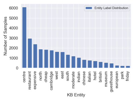
Figure 1. Entity label distribution on benchmark dataset MultiWOZ. X-axis denotes the top-20 most frequent entities in the system responses. Y-axis denotes the number of samples containing each entity.

We experiment with two popular types of dialogue models based on GPT (SimpleTOD (Hosseini-Asl et al., 2020)) and recurrent networks (GLMP (Wu et al., 2019b)). We evaluate using Entity F1 (Eric et al., 2017) and BLEU (Papineni et al., 2002) metrics which are the two main metrics for assessing the performance of dialogue models. F1 measures the accuracy of the system’s ability to extract the correct entities from the knowledge base, while BLEU measures how much word overlap between the system-generated response and the ground truth response; higher score means better performance in both metrics. The results are shown in Table 1. As we can see, both models perform similarly under the two training settings, implying that there are shortcuts in the data (i.e., frequent phrases that correlate strongly with entities and responses), and the model has learned to exploit these cues for the task. Manual analysis reveals that 87% of the frequent phrases do not contain much semantic information: most of them are made up of function words such as I’m looking for, I would like, I don’t care, and That is all. These results suggest that these models did not solve the task by having any real natural language understanding.

Next we look into class imbalance, another source of dataset biases (Branco et al., 2021). We analyze the distribution of KB entities in the system responses, i.e., we tally how often each entity appears in the responses in MultiWOZ and plot a histogram of their frequencies in Figure 1. We find that the entity distribution is highly skewed, with the top-10 “head entities” (i.e., the most frequent entities) accounting for approximately 64% of total occurrences, which means a large portion of the entities are in the (very) long tail of the distribution. The implication is that a model can simply focus on learning from a small number of head entities to achieve a high performance. Motivated by this observation, we adapt filtering algorithms to tackle this class imbalance issue, which works by smoothing the distribution so as to encourage our model to learn not only from the head of the distribution but also from the tail.

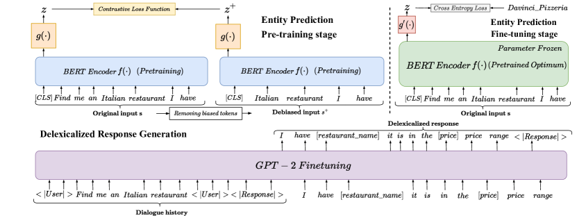
Figure 2. Overview of our proposed approach. The top shows the two-stage design for entity prediction: BERT pre-training using contrastive loss and fine-tuning using cross-entropy loss. The bottom shows the delexicalized response generation by fine-tuning GPT-2.

4. Model Architecture

4.1. Problem Formulation

We focus on the problem of task-oriented dialogue response generation with external knowledge base (KB). Formally, given the dialogue history $D$ and knowledge base $B$, our goal is to generate the system responses $Y$ in a word-by-word fashion. The probability of the generated responses can be written as:

$$\small p(Y|D,B)=\prod_{t=1}^{n}p(y_{t}|D,B,y_{1},y_{2},...,y_{t-1})$$

where $y_{t}$ is the t-th token in the response $Y$.

4.2. Overview

We decompose the dialogue generation task into two sub-tasks: delexicalized response generation and entity prediction. The delexicalized response is the response where KB entities are substituted by placeholders to reduce the complexity of the problem through a smaller vocabulary. For example, in Figure 2, Davinci Pizzeria is replaced by “[restaurant_name]” in the response. We follow the delexicalization process proposed in (Hosseini-Asl et al., 2020). We employ the two-phase design because it disentangles the entity prediction task from response generation task, allowing us to focus on bias reduction for entity prediction. Our framework uses a pre-trained autoregressive model (GPT-2) as the response generator and a pre-trained bidirectional encoder (BERT) as the entity predictor. Note that GPT-2 is fine-tuned to generate the delexicalized responses while the BERT model is fine-tuned to predict entities at every timestep during decoding, and the final response is created by replacing the placeholder tokens (generated by GPT-2) using the predicted entities (by BERT). Figure 2 presents the overall architecture. We first describe how the delexicalized response generation operates in Section 4.3 followed by entity prediction in Section 4.4. We introduce our debiasing techniques for the entity prediction model in Section 5.

4.3. Delexicalized Response Generation

We follow (Hosseini-Asl et al., 2020) and fine-tune GPT-2 to generate the delexicalized responses. Note that the input is always prefixed with the dialogue history and GPT-2 is fine-tuned via cross-entropy loss to predict the next (single turn) response.

4.4. Entity Prediction

The entity prediction task can be formulated as a multi-class classification problem. The goal of the entity prediction module is to predict the correct KB entities at each timestep during the response generation process, given the dialogue context and the generated word tokens before current timestep. Formally, let D = [$x_{1}$,$x_{2}$,…,$x_{n}$] be the dialogue history, Y = [$y_{1}$,$y_{2}$,…,$y_{m}$] be the ground truth delexicalized response, where $n$ is the number of tokens in the dialogue history, $m$ the number of tokens in the response. During training, we fine-tune BERT to predict the entity at the $t$-th timestep, by taking the dialogue history and the generated tokens, i.e., $\bar{D}$ = [$x_{1}$,$x_{2}$,…$x_{n}$,$y_{1}$,$y_{2}$,…,$y_{t-1}$], as the input:

$${H} ={BERT}_{{\scriptsize enc}}(\phi^{\scriptsize emb}({\bar{D}}))$$

$$z =g(H_{CLS})$$

$$P =\text{softmax}(z)$$

where $\phi^{\scriptsize emb}$ is the embedding layer of BERT, $H_{CLS}$ the hidden state of the [CLS] token, $g$ a linear layer, and $P$ the probability distribution over the KB entity set. Note that the KB entity set consists of all KB entities and a special label [NULL], which is used when the token to be predicted at timestep $t$ is not an entity (i.e., normal words). During inference, we use the delexicalized response generated by GPT-2 as input, and at each time step select the entity with the largest probability produced by BERT as the output.

The delexicalized response generator (GPT-2) and entity predictor (BERT) are trained separately, and at test time we first generate the delexicalized response and then use it as input to the entity predictor to predict the entities at every time step. Once that’s done, we lexicalize the response by substituting the placeholder tokens with their corresponding entities to create the final response.

5. Debiased Training For Robust Entity Prediction

Motivated by our preliminary findings a model that uses full input (I need to find a moderately priced hotel) performs similarly compared to one that uses filtered input containing only frequent phrases (I need to), we propose to use contrastive learning to encourage the entity predictor (BERT) to focus on the important semantic words, e.g., find a moderately priced hotel instead of I need to, during representation learning. We propose three methods leveraging $n$-gram statistics ($n=3$): frequency (Section 5.1.1), mutual information (Section 5.1.2), and Jensen-Shannon divergence (Section 5.1.3).

Our approach integrates contrastive learning in the domain-adaptive pre-training stage (Gururangan et al., 2020). That is, we take the off-the-shelf pre-trained BERT, and perform another step of pre-training to adapt it to our domain. Conventionally this domain-adaptive pre-training is done using masked language model loss, but we propose to use contrastive loss instead to encourage BERT to learn similar representations/encodings between the full input (I need to find a moderately priced hotel) and a debiased input (find a moderately priced hotel), thereby forcing the model to focus on the semantic words. After this contrastive pre-training, we fine-tune BERT for the entity prediction task as we described in Section 4.4.

Lastly, we also explore adapting an adversarial filtering algorithm (Sakaguchi et al., 2019) to further debias our model; this is detailed in Section 5.2.

5.1. Contrastive Learning

The core idea of contrastive learning is to learn representations where positive pairs are embedded in a similar space while negative pairs are pushed apart as much as possible (Gao et al., 2021; Khosla et al., 2021; van den Oord et al., 2019). We follow the contrastive learning framework in (Gao et al., 2021) that takes a set of paired utterances $S$ = $\{(s_{i},s_{i}^{+})\}^{N}_{i=1}$ as inputs, where $s_{i}$ denotes the original input and $s_{i}^{+}$ denotes its positive counterparts (i.e., the debiased utterances). It employs in-batch negatives and cross-entropy loss for training. Formally, the inputs $s_{i}$ and $s_{i}^{+}$ are first mapped into feature representations in vector space as $z_{i}$ and $z_{i}^{+}$. In our case we use BERT as our encoder to produce the features. The training loss $\mathcal{L}$ for $S$, a minibatch with $N$ pairs of utterances is:

$$\mathcal{L}=-\mathop{\mathbb{E}}\limits_{S}\left[log\frac{e^{\text{sim}(z_{i},z_{i}^{+})/\tau}}{\sum_{j=1}^{N}e^{\text{sim}(z_{i},z_{j}^{+})/\tau}}\right]$$

where $\tau$ is a temperature hyperparameter, $sim$ the cosine similarity function. The critical issue of contrastive learning is to construct a meaningful positive counterpart, which in our case means capturing the semantic bearing words in the original utterance. We next describe three ideas to construct the positive pairs based on $n$-gram statistics.

5.1.1. Criterion-1: Frequent $n$-grams

We select the top-10% $n$-grams according to their frequency in the training data, and create positive pairs containing: (1) an original input (dialogue history and response up to timestep $t-1$); and (2) filtered input where frequent $n$-grams are removed. As explained earlier in Section 5, this simple approach forces BERT to learn a similar representation between the full input (I need to find a moderately priced hotel) and debiased input (find a moderately priced hotel) by removing these $n$-grams directly.

5.1.2. Criterion-2: Mutual Information

The previous approach does not consider the label information (i.e., the entities contained in the responses). To incorporate label information, we explore computing mutual information between $n$-grams and the entities. The idea is that we want to discover $n$-grams that produce strong correlation with entities, which means that BERT is likely to pick them up as shortcuts for prediction. Formally:

$$I({A};{B})=\mathop{\sum}\limits_{A,B}p({A},{B})log\frac{p({A|B)}}{p({A})}$$

where ${A}$ is an $n$-gram and ${B}$ a target entity.

We rank all pairs of $n$-grams and entities this way, and select the top-10% pairs and use their $n$-grams (ignoring the entities) as the candidate set where we remove them in the input to create the positive pairs as before. The detailed algorithm is shown in Algorithm 1.

5.1.3. Criterion-3: Jensen-Shannon Divergence

The previous approach accounts for label (entity) information, but has the limitation where it considers only the presence of an $n$-gram with a target entity. Here we extend the approach to also consider the absence of the $n$-gram, and what impacts this brings to the appearance of the target entity. To this end we compute the Jensen-Shannon divergence of two probability distributions: (1) entity distribution where an $n$-gram is present in the input ($P$); and (2) entity distribution where an $n$-gram is absent in the input ($Q$). The idea is that an $n$-gram is highly informative (in terms of predicting the entities) if the divergence of the distributions is high, and we want to remove these $n$-grams from the input. Formally:

$$JSD({P};{Q})=\frac{1}{2}\sum_{x\in\mathbb{X}}{P}(x)log\frac{{P}(x)}{{M}(x)}+\frac{1}{2}\sum_{x\in\mathbb{X}}{Q}(x)log\frac{{Q}(x)}{{M}(x)}$$

where ${P}$ and ${Q}$ are two probability distributions over $\mathbb{X}$, ${M}$ = 1/2 (${P}$+${Q}$). Details about the algorithm are shown in Algorithm 2. As before, we select the top-10% $n$-grams ranked by the divergence values as the candidate $n$-grams to filter in the input.

1

Input : dataset $\mathcal{D}$ = ($\mathbf{X},\mathbf{y}$), $n$-gram size n, cutoff size k

Output : biased tokens set $\mathcal{S}$

2

3Initialize $n$-grams distribution $\mathbf{\textit{P}}_{ngrams}$ $\leftarrow$ $\emptyset$;

4 Initialize entity distribution $\mathbf{\textit{P}}_{entity}$ $\leftarrow$ $\emptyset$;

5 Initialize ngrams-entity joint distribution $\mathbf{\textit{P}}_{joint}$ $\leftarrow$ $\emptyset$;

6 Initialize mutual information values Q $\leftarrow$ $\emptyset$;

7 foreach $(x,y)\in(\mathbf{X},\mathbf{y})$ do

8       $ngrams$ $\leftarrow$ FindNgrams(x, n);

9       foreach element $e$ of the $ngrams$ do Add $e$ to $\mathbf{\textit{P}}_{ngrams}$;

10       Add $y$ to $\mathbf{\textit{P}}_{entity}$;

11       forall $e\in ngrams$ do Add ($e,y$) to $\mathbf{\textit{P}}_{joint}$;

12      

13 end foreach

14forall $(e_{1},e_{2})\in\mathbf{\textit{P}}_{joint}$ do

15       Calculate mutual information $m$ of ($e_{1},e_{2}$) using $\mathbf{\textit{P}}_{ngrams}$, $\mathbf{\textit{P}}_{entity}$, $\mathbf{\textit{P}}_{joint}$ with Equation 5.1.2;

16       Add ($e_{1},e_{2},m$) to $Q$;

17      

18 end forall

19Select the top-k elements $\mathcal{F}$ of $Q$ and Add $\mathcal{F}$($e_{1}$) to $\mathcal{S}$;

return $\mathcal{S}$

Algorithm 1 Mutual information based bias identification

1

Input : dataset $\mathcal{D}$ = ($\mathbf{X},\mathbf{y}$), $n$-gram size n, cutoff size k

Output : biased tokens set $\mathcal{S}$

2

3Initialize $n$-grams set $\mathbf{\textit{S}}_{ngrams}$ $\leftarrow$ $\emptyset$;

4 Initialize positive entity distribution $\mathbf{\textit{P}}_{positive}$ $\leftarrow$ $\emptyset$;

5 Initialize negative entity distribution $\mathbf{\textit{P}}_{negative}$ $\leftarrow$ $\emptyset$;

6 Initialize JSD values Q $\leftarrow$ $\emptyset$;

7 foreach $x\in\mathbf{X}$ do

8       $ngrams$ $\leftarrow$ FindNgrams(x, n);

9       foreach element $e$ of the $ngrams$ do Add $e$ to $\mathbf{\textit{S}}_{ngrams}$;

10      

11 end foreach

12foreach $(x,y)\in(\mathbf{X},\mathbf{y})$ do

13       foreach $e\in ngrams$ do

14             if $e\in x$ then Add ($e,y$) to $\mathbf{\textit{P}}_{positive}$;

15             else Add ($e,y$) to $\mathbf{\textit{P}}_{negative}$;

16            

17       end foreach

18      

19 end foreach

20foreach $e\in\mathbf{\textit{S}}_{ngrams}$ do

21       Calculate JSD values $v$ for $e$ using $\mathbf{\textit{P}}_{positive}$, $\mathbf{\textit{P}}_{negative}$ with Equation 5.1.3;

22       Add ($e,v$) to $Q$;

23      

24 end foreach

25Select the top-k elements $\mathcal{F}$ of $Q$ and Add $\mathcal{F}$($e$) to $\mathcal{S}$;

return $\mathcal{S}$

Algorithm 2 JSD based bias identification

5.2. Adversarial Filtering

Contrastive pre-training identifies and eliminates biased tokens at the input representation level. However, this does not change the entity label distribution, which is another source of bias that makes deep learning models brittle to unseen scenarios (Peng et al., 2020b; Liu et al., 2021). To address this, we adapt the adversarial filtering proposed by (Sakaguchi et al., 2019) to smooth the entity label distribution to prevent the model from learning only from the head of the distribution (frequent entities) but also from the tail of the distribution (rarer entities). The core idea of adversarial filtering is to filter out “easy” training examples — training instances where their removal doesn’t negatively impact the model — to encourage the model to learn from the “hard” examples, through an iterative process utilizing weak linear learners.

During each iteration, we train 100 linear classifiers (logistic regression) on a randomly sampled subset (30%) of training instances. When the training of each classifier converges, we use it to make predictions for the remaining 70% instances and record their predictions. At the end of each iteration, we compute the average prediction accuracy for each instance by calculating the ratio of correct predictions over all classifiers, and filter out instances that have a prediction accuracy $>=0.75$ and repeat the process with the remaining instances for the next iteration. The algorithm terminates when less than 500 instances are filtered during one iteration or when it has reached 100 iterations. After the filtering process, any instances that are not filtered are used for to further fine-tune the entity predictor (BERT). Note that we apply this fine-tuning on the best model (based on validation) from contrastive learning (Section 5.1), and following previous studies (Tian et al., 2020; Chen et al., 2020; Khosla et al., 2021) we freeze the BERT parameters and initialise (randomly) a new linear layer.

Model	Original		WP		WD		SP		SI
	F1	BLEU	F1	BLEU	F1	BLEU	F1	BLEU	F1	BLEU
Mem2Seq (Madotto et al., 2018)	23.42	4.53	7.69	3.94	8.20	3.91	9.65	4.17	10.25	4.06
GLMP (Wu et al., 2019b)	33.79	6.22	10.21	5.34	10.97	5.29	13.14	5.69	14.04	5.53
DF-Net (Qin et al., 2020)	35.73	7.01	11.02	6.08	11.73	6.03	14.01	6.45	14.96	6.28
SimpleTOD (Hosseini-Asl et al., 2020)	35.80	20.20	11.19	9.25	12.02	9.19	14.37	10.63	15.35	10.45
$\textup{Ours (w/o CL, w/ MLM)}^{\diamondsuit}$	36.74	21.05	11.33	10.99	12.67	10.97	15.01	11.53	16.47	12.24
$\textup{Ours (w/ CL, Frequent $n$-grams)}^{\spadesuit}$	32.20	20.61	27.85	17.87	26.66	17.23	26.44	16.33	19.90	16.04
$\textup{Ours (w/ CL, Mutual Information)}^{\spadesuit}$	31.86	20.04	28.84	18.38	26.98	17.36	27.14	16.60	23.60	16.89
$\textup{Ours (w/ CL, Jensen-Shannon Divergence)}^{\spadesuit}$	31.50	19.42	29.15	18.96	28.13	18.33	28.95	17.81	23.96	17.37
$\textup{Ours (w/o CL, w/ AF)}^{\heartsuit}$	31.35	20.37	27.22	17.80	26.51	17.57	26.04	17.14	21.30	16.49
$\textup{Ours (w/ CL, w/ AF)}^{\heartsuit}$	30.98	19.26	29.89	19.01	29.28	18.93	29.20	18.06	28.69	17.59

Table 2. Adversarial attack results. All the models are trained on the original (unperturbed) MultiWOZ data using all domains. “Original” denote the original MultiWOZ test set, while “WP”, “WD”, “SP” and “SI” denote adversarial test sets created through word paraphrasing, word deletion, sentence paraphrasing and sentence insetion respectively, using NlpAug (Ma, 2019). $\diamondsuit$: Our vanilla model without contrastive learning or adversarial filtering; $\spadesuit$: our model with contrastive learning; $\heartsuit$: our model with adversarial filtering.

6. Experiments

To verify the effectiveness of our proposed debiasing approach, we conduct a comprehensive study comparing our model against a number of benchmark systems. Our experiments include cross-domain/dataset generalization test, adversarial samples (created by distorting words and sentences), and utterances featuring unseen $n$-grams.

6.1. Datasets and Metrics

We use MultiWOZ (Eric et al., 2019) as the main dialogue dataset for our experiments. Specifically, we use version 2.2 of the dataset (Zang et al., 2020) which fixes a number of annotation errors and disallows slots with a large number of values to improve data quality. For evaluation metrics, we use the same BLEU and Entity F1 measures that we used in our preliminary investgation (Section 3).

6.2. Baselines

We compare our model against the following state-of-the-art benchmark systems:

• Mem2Seq (Madotto et al., 2018): employs a recurrent network-based decoder to generate system responses and utilize memory networks to store the KB and copy KB entities from memory via pointer mechanism. The decoder are jointly trained with memory networks end-to-end by maximizing the likelihood of the final system responses.

• GLMP (Wu et al., 2019b): employs a global-to-local pointer mechanism over the standard memory networks architecture for improving KB retrieval accuracy during response generation. The global pointer is supervised by additional training signals extracted from the standard system responses.

• DF-Net (Qin et al., 2020): utilizes a shared-private architecture to capture both domain-specific and domain-general knowledge to improve the model transferability.

• SimpleTOD (Hosseini-Asl et al., 2020): a causal language model based on GPT-2 trained on several task-oriented dialogue sub-tasks including dialogue state tracking, action prediction and response generation. It exploits additional training signals such as dialogue states and system acts compared to other systems.

6.3. Implementation Details

For delexicalized response generation, we use pretrained gpt2. We use the default hyper-parameter configuration, except for learning rate and batch size where we optimise via grid search. The learning rate is selected from {$1e^{-3}$,$1e^{-4}$,$1e^{-5}$, $2e^{-4}$,$2e^{-4}$,$2e^{-4}$} and batch size from {2,4,8,16,32} based on the best validation performance.

For entity prediction, we use pretrained bert-base-uncased. During contrastive pre-training stage, the learning rate is selected from {$1e^{-3}$,$1e^{-4}$, $1e^{-5}$,$1e^{-6}$} and batch size from {2,4,8,16,32} using grid search based on validation performance. We pre-train BERT with contrastive learning for 20 epochs. The model with the best validation performance (minimum loss) is used for fine-tuning for entity prediction. During fine-tuning stage, the learning rate is selected from {$1e^{-3}$,$1e^{-4}$,$1e^{-5}$,$2e^{-4}$, $2e^{-4}$,$2e^{-4}$} and the batch size from {2,4,8,16,32}. We use Adam (Kingma and Ba, 2014) as the optimizer. In terms of $n$-gram order, $n=3$ (trigram).

We run all experiments five times using different random seeds and report the average and standard deviation. All the models are trained on a single GeForce RTX 2080 Ti GPU and the training of both components (response generator and entity predictor) takes approximately one day.

Model All All Restaurant Hotel Attraction Training F1 BLEU F1 F1 F1 F1 Mem2Seq (Madotto et al., 2018) 10.38 ($\pm$0.28) 4.27 ($\pm$0.79) 13.51 ($\pm$0.13) 5.59 ($\pm$0.26) 14.85 ($\pm$0.30) 8.66 ($\pm$0.50) GLMP (Wu et al., 2019b) 14.25 ($\pm$0.20) 5.84 ($\pm$0.05) 18.93 ($\pm$0.42) 7.06 ($\pm$0.47) 20.95 ($\pm$0.29) 11.67 ($\pm$0.20) DF-Net (Qin et al., 2020) 15.17 ($\pm$0.31) 6.61 ($\pm$0.41) 20.10 ($\pm$0.20) 7.61 ($\pm$0.30) 22.23 ($\pm$0.43) 12.46 ($\pm$0.29) SimpleTOD (Hosseini-Asl et al., 2020) 15.57 ($\pm$0.17) 12.79 ($\pm$0.25) 20.64 ($\pm$0.12) 7.78 ($\pm$0.10) 22.83 ($\pm$0.30) 12.78 ($\pm$0.14) $\textup{Ours (w/o CL, w/ MLM)}^{\diamondsuit}$ 15.82 ($\pm$0.46) 14.36 ($\pm$0.21) 18.04 ($\pm$0.09) 8.68 ($\pm$0.11) 23.16 ($\pm$0.19) 14.49 ($\pm$0.47) $\textup{Ours (w/ CL, Frequent $n$-grams)}^{\spadesuit}$ 20.33 ($\pm$0.15) 17.17 ($\pm$0.15) 22.29 ($\pm$0.09) 10.23 ($\pm$0.21) 20.82 ($\pm$0.12) 9.65 ($\pm$0.02) $\textup{Ours (w/ CL, Mutual Information)}^{\spadesuit}$ 21.25 ($\pm$0.04) 17.86 ($\pm$0.05) 20.80 ($\pm$0.05) 12.91 ($\pm$0.31) 26.05 ($\pm$0.28) 13.72 ($\pm$0.16) $\textup{Ours (w/ CL, Jensen-Shannon Divergence)}^{\spadesuit}$ 26.42 ($\pm$0.14) 21.83 ($\pm$0.07) 28.46 ($\pm$0.15) 14.72 ($\pm$0.07) 27.07 ($\pm$0.12) 15.64 ($\pm$0.04) $\textup{Ours (w/o CL, w/ AF)}^{\heartsuit}$ 20.26 ($\pm$0.11) 15.53 ($\pm$0.25) 20.30 ($\pm$0.08) 10.04 ($\pm$0.06) 24.31 ($\pm$0.04) 14.22 ($\pm$0.19) $\textup{Ours (w/ CL, w/ AF)}^{\heartsuit}$ 29.80 ($\pm$0.27) 22.05 ($\pm$0.15) 27.51 ($\pm$0.37) 22.59 ($\pm$0.17) 40.07 ($\pm$0.09) 15.72 ($\pm$0.28)

Table 3. Unseen utterances generalization test results. All the training and inference are done on the new train/test splits (see Section 6.5) created to reduce $n$-gram overlap between training and test data. “F1 (All)”: testing F1 using all the domains; “BLEU (All)”: testing BLEU using all the domains; “Training F1”: F1 results on training partition using all the domains. We run each experiment five times with different random seeds and report the average results with standard deviation (in parenthesis).

6.4. Adversarial Attack Results

Language variety is one of the key features of human languages (Ganhotra et al., 2020), i.e., we tend to express the same meaning using different words. In real-world situations, users may use very different expressions than those in the training data. To test model robustness under such situations, we perform several perturbations on user utterances in the original test set to construct adversarial test examples. We use the widely-used NlpAug library (Ma, 2019) to augment the “regular” user utterances to generate four adversarial test sets through: word paraphrasing (WP), word deletion (WD), sentence paraphrasing (SP), and sentence insertion (SI). All the hyper-parameters of the augmentation tool NlpAug are kept to their default. We train all systems (benchmark and ours) using the original MultiWOZ and test them on both the original test set and adversarial test sets. Results are shown in Table 2 .

Our model has several variants: (1) vanilla without any debiasing, noting that it still has domain adaptive pre-training using the masked language model loss ($\diamondsuit$); (2) with contrastive loss for domain-adaptive pre-training ($\spadesuit$); and (3) with adversarial filtering, applied with or without contrastive pre-training ($\heartsuit$). The reason why our vanilla model has masked language model pre-training is that we need to understand that when we introduce contrastive pre-training, any performance gain is attributed to the contrastive learning objective rather than the domain adaptive pre-training step.

Looking at the original test set (“Original”), among the benchmark systems SimpleTOD is the best model, and our vanilla model ($\diamondsuit$) performs similarly (marginally better F1 but lower BLEU). Introducing contrastive learning ($\spadesuit$) and adversarial filtering ($\heartsuit$) somewhat degrades the entity prediction performance (F1), although the quality of the generated response (BLEU) is less impacted. Moving on to the adversarial test sets, all benchmark systems and our vanilla model observe severe performance degradation: F1 drops by over 20 points and BLEU by 10 points for most systems, suggesting that these models are not robust against perturbed inputs. Our systems with contrastive learning and/or adversarial filtering, on the other hand, look promising: the drop is substantially less severe, 2-3 points in terms of F1 and BLEU. Interestingly, we also see that SI appears to be the most challenging test set as its performance is lowest. Comparing the three different criteria for ranking $n$-grams (frequent $n$-gram, mutual information and Jensen-Shannon divergence), Jensen-Shannon divergence appears to have the upper hand, suggesting that label information and both the presence and absence of an $n$-gram is important for uncovering shortcuts in the data.

Model Hotel,Attraction,Train Restaurant,Attraction,Train Restaurant,Hotel,Train Restaurant,Hotel,Attraction $\rightarrow$ Restaurant $\rightarrow$ Hotel $\rightarrow$ Attraction $\rightarrow$ Train F1 BLEU F1 BLEU F1 BLEU F1 BLEU Mem2Seq (Madotto et al., 2018) 9.70 ($\pm$0.04) 4.88 ($\pm$0.56) 2.87 ($\pm$0.30) 3.89 ($\pm$0.48) 6.97 ($\pm$0.16) 3.67 ($\pm$0.66) 2.89 ($\pm$0.08) 3.03 ($\pm$0.05) GLMP (Wu et al., 2019b) 13.22 ($\pm$0.36) 6.75 ($\pm$0.09) 2.98 ($\pm$0.47) 5.26 ($\pm$0.51) 9.13 ($\pm$0.40) 4.94 ($\pm$0.11) 3.00 ($\pm$0.19) 3.98 ($\pm$0.26) DF-Net (Qin et al., 2020) 14.09 ($\pm$0.69) 7.57 ($\pm$0.04) 3.32 ($\pm$0.38) 5.99 ($\pm$0.49) 9.79 ($\pm$0.58) 5.66 ($\pm$0.10) 3.34 ($\pm$0.24) 4.65 ($\pm$0.52) SimpleTOD (Hosseini-Asl et al., 2020) 14.46 ($\pm$0.47) 13.78 ($\pm$0.40) 3.36 ($\pm$0.08) 11.16 ($\pm$0.27) 10.03 ($\pm$0.15) 11.82 ($\pm$0.09) 3.38 ($\pm$0.45) 13.77 ($\pm$0.39) $\textup{Ours (w/o CL, w/ MLM)}^{\diamondsuit}$ 14.95 ($\pm$0.35) 14.23 ($\pm$0.07) 5.80 ($\pm$0.02) 13.81 ($\pm$0.11) 10.31 ($\pm$0.19) 12.93 ($\pm$0.42) 3.77 ($\pm$0.34) 14.91 ($\pm$0.03) $\textup{Ours (w/ CL, Frequent $n$-grams)}^{\spadesuit}$ 19.09 ($\pm$0.20) 15.27 ($\pm$0.07) 12.34 ($\pm$0.27) 14.56 ($\pm$0.09) 13.62 ($\pm$0.14) 14.32 ($\pm$0.26) 10.25 ($\pm$0.41) 14.93 ($\pm$0.06) $\textup{Ours (w/ CL, Mutual Information)}^{\spadesuit}$ 22.24 ($\pm$0.19) 15.33 ($\pm$0.26) 14.85 ($\pm$0.35) 14.60 ($\pm$0.14) 15.05 ($\pm$0.26) 15.93 ($\pm$0.44) 11.76 ($\pm$0.08) 17.46 ($\pm$0.47) $\textup{Ours (w/ CL, Jensen-Shannon Divergence)}^{\spadesuit}$ 23.14 ($\pm$0.25) 15.68 ($\pm$0.13) 18.01 ($\pm$0.38) 15.01 ($\pm$0.25) 19.61 ($\pm$0.47) 16.38 ($\pm$0.07) 12.48 ($\pm$0.32) 18.86 ($\pm$0.44) $\textup{Ours (w/o CL, w/ AF)}^{\heartsuit}$ 21.30 ($\pm$0.17) 16.35 ($\pm$0.14) 15.26 ($\pm$0.33) 14.96 ($\pm$0.48) 16.76 ($\pm$0.41) 16.12 ($\pm$0.18) 10.86 ($\pm$0.31) 16.30 ($\pm$0.11) $\textup{Ours (w/ CL, w/ AF)}^{\heartsuit}$ 25.13 ($\pm$0.29) 17.93 ($\pm$0.35) 23.86 ($\pm$0.17) 15.83 ($\pm$0.12) 21.37 ($\pm$0.20) 16.90 ($\pm$0.09) 14.43 ($\pm$0.13) 19.03 ($\pm$0.08)

Table 4. Cross-domain generalization results. “X$\rightarrow$Y”: X denote the training domain(s) and Y the test domain.

Model	MultiWOZ$\to$SMD		MultiWOZ$\to$SGD
	F1	BLEU	F1	BLEU
Mem2Seq (Madotto et al., 2018)	9.06 ($\pm$0.49)	8.01 ($\pm$0.33)	4.34 ($\pm$0.28)	3.48 ($\pm$0.63)
GLMP (Wu et al., 2019b)	12.25 ($\pm$0.21)	11.45 ($\pm$0.74)	5.18 ($\pm$0.47)	4.66 ($\pm$0.38)
DF-Net (Qin et al., 2020)	13.07 ($\pm$0.71)	12.51 ($\pm$0.57)	5.63 ($\pm$0.79)	5.36 ($\pm$0.94)
SimpleTOD (Hosseini-Asl et al., 2020)	13.41 ($\pm$0.41)	13.87 ($\pm$0.37)	5.75 ($\pm$0.81)	7.51 ($\pm$0.29)
$\textup{Ours (w/o CL, w/ MLM)}^{\clubsuit}$	13.57 ($\pm$0.44)	14.45 ($\pm$0.69)	6.06 ($\pm$0.77)	8.94 ($\pm$0.76)
$\textup{Ours (w/ CL, Frequent $n$-grams)}^{\spadesuit}$	19.01 ($\pm$0.70)	15.25 ($\pm$0.44)	9.44 ($\pm$0.78)	10.07 ($\pm$0.73)
$\textup{Ours (w/ CL, Mutual Information)}^{\spadesuit}$	20.32 ($\pm$0.42)	15.44 ($\pm$0.15)	9.79 ($\pm$0.81)	10.38 ($\pm$0.76)
$\textup{Ours (w/ CL, Jensen-Shannon Divergence)}^{\spadesuit}$	21.80 ($\pm$0.68)	15.70 ($\pm$0.67)	11.23 ($\pm$0.14)	10.68 ($\pm$0.07)
$\textup{Ours (w/o CL, w/ AF)}^{\heartsuit}$	20.44 ($\pm$0.39)	15.43 ($\pm$0.62)	9.73 ($\pm$0.04)	10.25 ($\pm$0.11)
$\textup{Ours (w/ CL, w/ AF)}^{\diamondsuit}$	23.79 ($\pm$0.49)	18.25 ($\pm$0.23)	11.41 ($\pm$0.21)	10.99 ($\pm$0.05)

Table 5. Cross-dataset generalization results. “A$\rightarrow$B”: a model is trained using train partition of dataset A and evaluated on the test partition of dataset B in a zero-shot manner.

6.5. Unseen Utterances Generalization Results

To test our model’s generalization capability under unseen scenario, we construct a new MultiWOZ split that aims to reduce $n$-gram overlap between training and test data. We first collect all $n$-gram types in the full data (training $+$ test) and remove low frequency ($<10$) $n$-grams , and then create two sets of $n$-grams based on their frequencies: “train” which contains the most frequent (70%) $n$-gram types and “test” for the remaining (30%). These two sets will decide whether an instance will be assigned to the training or test partition. That is, we iterate each instance from the full data and put it to the training partition if it only contains “train” $n$-gram, or the test partition if it has only “test” $n$-gram.

Empirically, in the original MultiWOZ split the $n$-gram overlap ratio is 82.75%; our new split reduces this to 51.2%. This means that during testing, a model using our split will be exposed to utterances with more unseen phrases, and if the model exploits the spurious cues ($n$-grams) in the input it will likely to perform poorly under this new split, as these cues are more likely to be absent.

We train all models using the new training partition and test them on the new test partition and present the results in Table 3. Looking at the models without debiasing, we find a similar observation where SimpleTOD and our vanilla model ($\diamondsuit$) are the best performing models over different domains. When we introduce contrastive learning ($\spadesuit$) and adversarial filtering ($\heartsuit$), we see an improvement over all domains, with the best variant that combines both (“w/ CL, w/ AF”) improving over the vanilla model by a large margin, about 14% in Entity F1 and 8% in BLEU. As before, using Jensen-Shannon divergence as the criterion for ranking $n$-grams turns out to be the best approach. Contrastive learning and adversarial filtering seem to provide complementary signal based on this experiment, as combining them both produces substantially better performance.

To understand how these two methods complement each other, we present F1 performance in the training partition (last column in Table 3): here we see that the models that are not debiased have similar training and test performance, while the contrastive models ($\spadesuit$) have a much lower training performance, suggesting there is underfitting. Adversarial filtering, however, does not suffer from this problem (“w/o CL, w/ AF”), as it only removes training instances that do not negatively impact training accuracy. Interestingly, when we incorporate adversarial filtering to the contrastive model (“w/ CL, w/ AF”), this underfitting problem is corrected, showing their complementarity.

6.6. Cross-domain Generalization Results

We now test cross-domain generalization, where a model is tested using a domain that is not in the training data.

We use the “leave-one-out” strategy for this, where a model is trained using all except one domain and tested using that unseen domain. We present the results in Table 4.

We see similar observations here. Without any debiasing, SimpleTOD and our vanilla have the best performances. When we incorporate contrastive learning and adversarial filtering, we see a strong improvement in terms of model robustness. As before, the best variant is one that combines both, and when compared to the vanilla model it improves F1 by 10–18 and BLEU by 2–5 points depending on the test domain. For contrastive learning, Jensen-Shanon divergence is again the best criterion for selecting $n$-grams. Adversarial filtering by itself is also fairly effective, although not as effective as the best contrastive model.

6.7. Cross-dataset Results

We now test the hardest setting: cross-dataset generalization. If a model “overfits” a dataset and relies on spurious correlations to perform a task, it will likely to perform very poorly in a new dataset of the same task. In this experiment, we train systems on MultiWOZ, and test them on two other popular datasets for task-oriented dialogues: SMD (Eric et al., 2017) and SGD (Rastogi et al., 2020). For SGD, it doesn’t have a database like SMD and MultiWOZ. Following (Rastogi et al., 2020), we collect the returned entities from the API queries during each dialogue as the database records to mimic the data settings of SMD and MultiWOZ.

The results are shown in Table 5. Both contrastive learning and adversarial filtering are effective methods to improve model robustness. The best contrastive model (“w/ Jensen-Shanon divergence”) improves F1 by 5–8 and BLEU by 1–2 points when compared to the vanilla model. Adversarial filtering by itself is also effective, although the improvement is marginally smaller compared to the best contrastive model. Once again, combining both produces the best performance. SGD is noticeably a harder dataset here, where F1 performance of all models is about half of SMD’s.

All in all these generalization tests reveal strikingly similar observations. To summarize: (1) our vanilla model that decomposes task-oriented dialogue generation into delexicalized response generation and entity prediction performs competitively with benchmark systems; (2) for contrastive learning, Jensen-Shannon divergence is consistently the best performer for ranking $n$-grams, implying that it is important to consider both the absence and presence of $n$-grams when determining their correlations with the labels; and (3) contrastive learning and adversarial filtering complement each other, and the most robust model is produced by incorporating both methods. Note that although our experiments focus on task-oriented dialogue, our methodology can be adapted to other NLP tasks without much difficulty. We believe that our contrastive pre-training method is likely useful to reduce general NLP data artifacts, as spurious correlations between words and labels are likely to surface during data development.

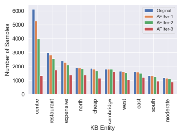
Figure 3. Change in entity frequency over different iterations of adversarial filtering. X-axis shows the 10 most frequent entity labels in the response. Y-axis shows the frequency of training instances for an entity. “Original”: Entity frequency without any filtering; “AF Iter-k”: Entity frequency after k iterations of filtering.

6.8. Adversarial Filtering Dynamics Analysis

The adversarial filtering iteratively detects the easy training instances and remove them. A natural question to ask is: why does this filtering process make the model more robust? To answer this question, we perform an analysis on the dynamics of the iterative process where we analyzed the number of instances containing a particular entity. We select the top-10 most frequent entities in the response and monitor their change in frequency over the iterations and present the results in Figure 3. As we can see from the figure, the distribution over these 10 entities has become “flatter” after the third iteration (red bars). The more frequent an entity is, the more instances are removed: at the extreme, the most frequent entity (centre) has lost almost 5000 instances after 3 iterations of filtering. Intuitively, we believe the more balanced distribution disincentivizes the model to focus on shortcuts that produce the frequent labels (entities), resulting in a model that learns generalisable patterns from a larger set of entities in the tail of the distribution.

7. Conclusion

In this work, we investigate data artifacts in MultiWOZ, a popular task-oriented dialogue dataset. We find that a model that uses full input for training performs similarly to a variant that uses partial input containing only frequent phrases, suggesting that there are data artifacts and the model uses them as shortcuts for the task. Motivated by this analysis, we propose a contrastive learning objective to debias task-oriented dialogue models by encouraging models to ignore these frequent phrases to focus on semantic words in the input. We also adapt adversarial filtering to our task to further improve model robustness. We conduct a series of generalization experiments, testing our method and a number of state-of-the-art benchmarks. Experimental results show that contrastive learning and adversarial filtering complement each other, and combining both produces the most robust dialogue model.

References

- (1)
- Belinkov et al. (2019) Yonatan Belinkov, Adam Poliak, Stuart M. Shieber, Benjamin Van Durme, and Alexander M. Rush. 2019. Don’t Take the Premise for Granted: Mitigating Artifacts in Natural Language Inference. arXiv:1907.04380 [cs.CL]
- Bordes et al. (2017) Antoine Bordes, Y-Lan Boureau, and Jason Weston. 2017. Learning End-to-End Goal-Oriented Dialog.. In ICLR. http://dblp.uni-trier.de/db/conf/iclr/iclr2017.html#BordesBW17
- Branco et al. (2021) Ruben Branco, António Branco, João António Rodrigues, and João Ricardo Silva. 2021. Shortcutted Commonsense: Data Spuriousness in Deep Learning of Commonsense Reasoning. In Proceedings of the 2021 Conference on Empirical Methods in Natural Language Processing. Association for Computational Linguistics, Online and Punta Cana, Dominican Republic, 1504–1521. https://doi.org/10.18653/v1/2021.emnlp-main.113
- Budzianowski et al. (2018) Paweł Budzianowski, Tsung-Hsien Wen, Bo-Hsiang Tseng, Iñigo Casanueva, Stefan Ultes, Osman Ramadan, and Milica Gasic. 2018. MultiWOZ-A Large-Scale Multi-Domain Wizard-of-Oz Dataset for Task-Oriented Dialogue Modelling. In Proceedings of the 2018 Conference on Empirical Methods in Natural Language Processing. 5016–5026.
- Chen et al. (2020) Ting Chen, Simon Kornblith, Mohammad Norouzi, and Geoffrey Hinton. 2020. A Simple Framework for Contrastive Learning of Visual Representations. arXiv:2002.05709 [cs.LG]
- Chen et al. (2019) Wenhu Chen, Jianshu Chen, Pengda Qin, Xifeng Yan, and William Yang Wang. 2019. Semantically Conditioned Dialog Response Generation via Hierarchical Disentangled Self-Attention. In Proceedings of the 57th Annual Meeting of the Association for Computational Linguistics. 3696–3709. https://doi.org/10.18653/v1/P19-1360
- Chen et al. (2016) Yun-Nung Chen, Dilek Hakkani-Tür, Gökhan Tür, Jianfeng Gao, and Li Deng. 2016. End-to-end memory networks with knowledge carryover for multi-turn spoken language understanding.. In Interspeech. 3245–3249.
- Devlin et al. (2018) Jacob Devlin, Ming-Wei Chang, Kenton Lee, and Kristina Toutanova. 2018. Bert: Pre-training of deep bidirectional transformers for language understanding. arXiv preprint arXiv:1810.04805 (2018).
- Devlin et al. (2019) Jacob Devlin, Ming-Wei Chang, Kenton Lee, and Kristina Toutanova. 2019. BERT: Pre-training of Deep Bidirectional Transformers for Language Understanding. In Proceedings of the 2019 Conference of the North American Chapter of the Association for Computational Linguistics: Human Language Technologies, Volume 1 (Long and Short Papers). 4171–4186.
- Eric et al. (2019) Mihail Eric, Rahul Goel, Shachi Paul, Abhishek Sethi, Sanchit Agarwal, Shuyag Gao, and Dilek Hakkani-Tur. 2019. Multiwoz 2.1: Multi-domain dialogue state corrections and state tracking baselines. arXiv preprint arXiv:1907.01669 (2019).
- Eric et al. (2017) Mihail Eric, Lakshmi Krishnan, Francois Charette, and Christopher D. Manning. 2017. Key-Value Retrieval Networks for Task-Oriented Dialogue. In Proceedings of the 18th Annual SIGdial Meeting on Discourse and Dialogue. 37–49. https://www.aclweb.org/anthology/W17-5506
- Ganhotra et al. (2020) Jatin Ganhotra, Robert Moore, Sachindra Joshi, and Kahini Wadhawan. 2020. Effects of Naturalistic Variation in Goal-Oriented Dialog. arXiv:2010.02260 [cs.CL]
- Gao et al. (2021) Tianyu Gao, Xingcheng Yao, and Danqi Chen. 2021. SimCSE: Simple Contrastive Learning of Sentence Embeddings. arXiv:2104.08821 [cs.CL]
- Geva et al. (2019) Mor Geva, Yoav Goldberg, and Jonathan Berant. 2019. Are We Modeling the Task or the Annotator? An Investigation of Annotator Bias in Natural Language Understanding Datasets. arXiv:1908.07898 [cs.CL]
- Ghazvininejad et al. (2018) Marjan Ghazvininejad, Chris Brockett, Ming-Wei Chang, Bill Dolan, Jianfeng Gao, Wen-tau Yih, and Michel Galley. 2018. A knowledge-grounded neural conversation model. In Thirty-Second AAAI Conference on Artificial Intelligence.
- Gururangan et al. (2020) Suchin Gururangan, Ana Marasović, Swabha Swayamdipta, Kyle Lo, Iz Beltagy, Doug Downey, and Noah A. Smith. 2020. Don’t Stop Pretraining: Adapt Language Models to Domains and Tasks. In Proceedings of the 58th Annual Meeting of the Association for Computational Linguistics. Online, 8342–8360.
- He et al. (2019) He He, Sheng Zha, and Haohan Wang. 2019. Unlearn Dataset Bias in Natural Language Inference by Fitting the Residual. arXiv:1908.10763 [cs.CL]
- Hendrycks et al. (2021) Dan Hendrycks, Kevin Zhao, Steven Basart, Jacob Steinhardt, and Dawn Song. 2021. Natural Adversarial Examples. arXiv:1907.07174 [cs.LG]
- Hosseini-Asl et al. (2020) Ehsan Hosseini-Asl, Bryan McCann, Chien-Sheng Wu, Semih Yavuz, and Richard Socher. 2020. A simple language model for task-oriented dialogue. arXiv preprint arXiv:2005.00796 (2020).
- Huang et al. (2019) Xiao Huang, Jingyuan Zhang, Dingcheng Li, and Ping Li. 2019. Knowledge graph embedding based question answering. In Proceedings of the Twelfth ACM International Conference on Web Search and Data Mining. ACM, 105–113.
- Ilyas et al. (2019) Andrew Ilyas, Shibani Santurkar, Dimitris Tsipras, Logan Engstrom, Brandon Tran, and Aleksander Madry. 2019. Adversarial Examples Are Not Bugs, They Are Features. arXiv:1905.02175 [stat.ML]
- Khosla et al. (2021) Prannay Khosla, Piotr Teterwak, Chen Wang, Aaron Sarna, Yonglong Tian, Phillip Isola, Aaron Maschinot, Ce Liu, and Dilip Krishnan. 2021. Supervised Contrastive Learning. arXiv:2004.11362 [cs.LG]
- Kingma and Ba (2014) Diederik P Kingma and Jimmy Ba. 2014. Adam: A method for stochastic optimization. arXiv preprint arXiv:1412.6980 (2014).
- Lei et al. (2018) Wenqiang Lei, Xisen Jin, Min-Yen Kan, Zhaochun Ren, Xiangnan He, and Dawei Yin. 2018. Sequicity: Simplifying Task-oriented Dialogue Systems with Single Sequence-to-Sequence Architectures. In Proceedings of the 56th Annual Meeting of the Association for Computational Linguistics.
- Liu et al. (2021) Jiexi Liu, Ryuichi Takanobu, Jiaxin Wen, Dazhen Wan, Hongguang Li, Weiran Nie, Cheng Li, Wei Peng, and Minlie Huang. 2021. Robustness Testing of Language Understanding in Task-Oriented Dialog. arXiv:2012.15262 [cs.CL]
- Ma (2019) Edward Ma. 2019. NLP Augmentation. https://github.com/makcedward/nlpaug.
- Madotto et al. (2018) Andrea Madotto, Chien-Sheng Wu, and Pascale Fung. 2018. Mem2Seq: Effectively Incorporating Knowledge Bases into End-to-End Task-Oriented Dialog Systems. In Proceedings of the 56th Annual Meeting of the Association for Computational Linguistics (Volume 1: Long Papers). 1468–1478. https://www.aclweb.org/anthology/P18-1136
- McCoy et al. (2019) R. Thomas McCoy, Ellie Pavlick, and Tal Linzen. 2019. Right for the Wrong Reasons: Diagnosing Syntactic Heuristics in Natural Language Inference. arXiv:1902.01007 [cs.CL]
- Niu et al. (2021) Yulei Niu, Kaihua Tang, Hanwang Zhang, Zhiwu Lu, Xian-Sheng Hua, and Ji-Rong Wen. 2021. Counterfactual VQA: A Cause-Effect Look at Language Bias. arXiv:2006.04315 [cs.CV]
- Niven and Kao (2019) Timothy Niven and Hung-Yu Kao. 2019. Probing Neural Network Comprehension of Natural Language Arguments. arXiv:1907.07355 [cs.CL]
- Papineni et al. (2002) Kishore Papineni, Salim Roukos, Todd Ward, and Wei-Jing Zhu. 2002. BLEU: a method for automatic evaluation of machine translation. In Proceedings of the 40th annual meeting on association for computational linguistics.
- Peng et al. (2020a) Baolin Peng, Chunyuan Li, Jinchao Li, Shahin Shayandeh, Lars Liden, and Jianfeng Gao. 2020a. SOLOIST: Building Task Bots at Scale with Transfer Learning and Machine Teaching. arXiv preprint arXiv:2005.05298 (2020).
- Peng et al. (2020b) Baolin Peng, Chunyuan Li, Zhu Zhang, Chenguang Zhu, Jinchao Li, and Jianfeng Gao. 2020b. RADDLE: An Evaluation Benchmark and Analysis Platform for Robust Task-oriented Dialog Systems. arXiv:2012.14666 [cs.CL]
- Peng et al. (2018) Baolin Peng, Xiujun Li, Jianfeng Gao, Jingjing Liu, and Kam-Fai Wong. 2018. Deep Dyna-Q: Integrating Planning for Task-Completion Dialogue Policy Learning. In Proceedings of the 56th Annual Meeting of the Association for Computational Linguistics (Volume 1: Long Papers). 2182–2192.
- Qi et al. (2020) Jiaxin Qi, Yulei Niu, Jianqiang Huang, and Hanwang Zhang. 2020. Two Causal Principles for Improving Visual Dialog. arXiv:1911.10496 [cs.CV]
- Qin et al. (2020) Libo Qin, Xiao Xu, Wanxiang Che, Yue Zhang, and Ting Liu. 2020. Dynamic Fusion Network for Multi-Domain End-to-end Task-Oriented Dialog. In Proceedings of the 58th Annual Meeting of the Association for Computational Linguistics. Association for Computational Linguistics, Online, 6344–6354. https://www.aclweb.org/anthology/2020.acl-main.565
- Radford et al. (2019) Alec Radford, Jeffrey Wu, Rewon Child, David Luan, Dario Amodei, Ilya Sutskever, et al. 2019. Language models are unsupervised multitask learners. OpenAI blog 1, 8 (2019), 9.
- Rastogi et al. (2020) Abhinav Rastogi, Xiaoxue Zang, Srinivas Sunkara, Raghav Gupta, and Pranav Khaitan. 2020. Towards Scalable Multi-domain Conversational Agents: The Schema-Guided Dialogue Dataset. arXiv:1909.05855 [cs.CL]
- Sakaguchi et al. (2019) Keisuke Sakaguchi, Ronan Le Bras, Chandra Bhagavatula, and Yejin Choi. 2019. WinoGrande: An Adversarial Winograd Schema Challenge at Scale. arXiv:1907.10641 [cs.CL]
- Sanh et al. (2020) Victor Sanh, Thomas Wolf, Yonatan Belinkov, and Alexander M. Rush. 2020. Learning from others’ mistakes: Avoiding dataset biases without modeling them. arXiv:2012.01300 [cs.CL]
- Tian et al. (2020) Yonglong Tian, Dilip Krishnan, and Phillip Isola. 2020. Contrastive Multiview Coding. arXiv:1906.05849 [cs.CV]
- van den Oord et al. (2019) Aaron van den Oord, Yazhe Li, and Oriol Vinyals. 2019. Representation Learning with Contrastive Predictive Coding. arXiv:1807.03748 [cs.LG]
- Veličković et al. (2017) Petar Veličković, Guillem Cucurull, Arantxa Casanova, Adriana Romero, Pietro Lio, and Yoshua Bengio. 2017. Graph attention networks. arXiv preprint arXiv:1710.10903 (2017).
- Wolf et al. (2019) Thomas Wolf, Victor Sanh, Julien Chaumond, and Clement Delangue. 2019. Transfertransfo: A transfer learning approach for neural network based conversational agents. arXiv preprint arXiv:1901.08149 (2019).
- Wu et al. (2020) Chien-Sheng Wu, Steven Hoi, Richard Socher, and Caiming Xiong. 2020. TOD-BERT: pre-trained natural language understanding for task-oriented dialogue. arXiv preprint arXiv:2004.06871 (2020).
- Wu et al. (2019a) Chien-Sheng Wu, Andrea Madotto, Ehsan Hosseini-Asl, Caiming Xiong, Richard Socher, and Pascale Fung. 2019a. Transferable Multi-Domain State Generator for Task-Oriented Dialogue Systems. arXiv preprint arXiv:1905.08743 (2019).
- Wu et al. (2019b) Chien-Sheng Wu, Richard Socher, and Caiming Xiong. 2019b. Global-to-local Memory Pointer Networks for Task-Oriented Dialogue.. In ICLR. http://dblp.uni-trier.de/db/conf/iclr/iclr2019.html#WuSX19
- Wu et al. (2016) Qi Wu, Peng Wang, Chunhua Shen, Anthony Dick, and Anton Van Den Hengel. 2016. Ask me anything: Free-form visual question answering based on knowledge from external sources. In Proceedings of the IEEE conference on computer vision and pattern recognition.
- Xing et al. (2018) Chen Xing, Yu Wu, Wei Wu, Yalou Huang, and Ming Zhou. 2018. Hierarchical recurrent attention network for response generation. In Thirty-Second AAAI Conference on Artificial Intelligence.
- Zang et al. (2020) Xiaoxue Zang, Abhinav Rastogi, Srinivas Sunkara, Raghav Gupta, Jianguo Zhang, and Jindong Chen. 2020. MultiWOZ 2.2 : A Dialogue Dataset with Additional Annotation Corrections and State Tracking Baselines. arXiv:2007.12720 [cs.CL]
- Zhang et al. (2020) Yichi Zhang, Zhijian Ou, and Zhou Yu. 2020. Task-oriented dialog systems that consider multiple appropriate responses under the same context. In Proceedings of the AAAI Conference on Artificial Intelligence, Vol. 34. 9604–9611.
- Zhang et al. (2019) Yizhe Zhang, Siqi Sun, Michel Galley, Yen-Chun Chen, Chris Brockett, Xiang Gao, Jianfeng Gao, Jingjing Liu, and Bill Dolan. 2019. Dialogpt: Large-scale generative pre-training for conversational response generation. arXiv preprint arXiv:1911.00536 (2019).
- Zhong et al. (2018) Victor Zhong, Caiming Xiong, and Richard Socher. 2018. Global-locally self-attentive dialogue state tracker. arXiv preprint arXiv:1805.09655 (2018).