Efficient Posterior Sampling For Diverse Super-Resolution with Hierarchical VAE Prior

Abstract

We investigate the problem of producing diverse solutions to an image super-resolution problem. From a probabilistic perspective, this can be done by sampling from the posterior distribution of an inverse problem, which requires the definition of a prior distribution on the high-resolution images. In this work, we propose to use a pretrained hierarchical variational autoencoder (HVAE) as a prior. We train a lightweight stochastic encoder to encode low-resolution images in the latent space of a pretrained HVAE. At inference, we combine the low-resolution encoder and the pretrained generative model to super-resolve an image. We demonstrate on the task of face super-resolution that our method provides an advantageous trade-off between the computational efficiency of conditional normalizing flows techniques and the sample quality of diffusion based methods.

1 INTRODUCTION

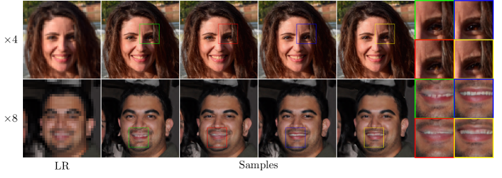
Figure 1: Diverse super-resolved samples at different upscaling factors. Our method can generate realistic samples with diverse attributes (hairs, mouth, eyes…).

Image super-resolution is the task of generating a high-resolution (HR) image $\bm{x}$ corresponding to a low-resolution (LR) observation $\bm{y}$. A typical approach for image super-resolution is to train a deep neural network in a supervised fashion to map a LR image to its HR counterpart (see [23] for an extensive review). Despite impressive performances, those regression based methods are fundamentally limited by their lack of diversity. Indeed, there might exist many plausible HR solutions associated with one LR observation, but regression based methods only provide one of those solutions.

An alternative approach for image super-resolution is to sample from the posterior distribution $p(\bm{x}|\bm{y})$. Specifically, we can train conditional deep generative models to fit the posterior $p(\bm{x}|\bm{y})$. With the recent advances in deep generative modeling, it is possible to generate realistic and diverse samples from the posterior distribution.

Starting from the seminal work of  [26], many approaches proposed to train conditional generative models such as conditional normalizing flow or conditional variational autoencoders in order to model the posterior distribution of the super-resolution problem. We refer to those methods as direct methods, as they only require one network function evaluation (NFE) to generate one sample.

With the recent development of score-based generative models (also known as denoising diffusion models) [16, 41], posterior sampling methods based on conditional denoising diffusion models are now able to produce high-quality samples outperforming previous direct methods [6, 7, 20]. However, denoising diffusion methods are limited by their computationally expensive sampling process, as they require numerous network function evaluations to generate one super-resolved sample. In the following, we classify those methods as iterative methods.

In this work, we address the question: Can we get the best of both worlds between the sampling quality of iterative methods, and the computationnal efficiency of direct methods? We show that it is indeed possible to reach this goal with our diverse super-resolution method CVDVAE (Conditional VDVAE).

Our approach is based on reusing a pretrained hierarchical variational autoencoder (HVAE) [39, 21]. HVAE models are able to generate high-quality images by relying on an expressive sequential generative model [42, 4, 15]. By associating one latent variable subgroup to each residual block of a generative network, HVAE models are able to learn compact high-level representations of the data, and they can generate new samples efficiently, with only one evaluation of the generative network.

The fast sampling time and the expressivity of HVAE models make them suitable candidates for efficient posterior sampling. In this work, we exploit a pretrained VD-VAE model [4]. In order to repurpose VD-VAE generative model for image super-resolution, we train a low-resolution encoder to encode LR images in the latent space of the VD-VAE model. By combining the LR encoder with the VD-VAE generative model, we can produce a sample with only one (autoencoder) network evaluation. By adopting a stochastic model for the LR encoder, our method can generate diverse samples from the posterior distribution, as illustrated in Figure 1. We show that the LR encoder can be trained with reasonable computational resources by exploiting the VD-VAE original (HR) encoder to generate labels for training the LR-encoder, and by sharing weights between the LR encoder and VD-VAE generative model. We evaluate our method on super-resolution of face images, with upscaling factor $\times 4$ and $\times 8$ and demonstrate that it reaches sample quality on par with sequential methods, while being significantly faster ($>\times 500$).

The paper is organised as follows. In section 2, we provide the necessary background on HVAE models. Then we present in section 3 our super-resolution method. Experimental results are given in section 4 and we discuss related works in section 5.

2 HIERARCHICAL VAE

Variational autoencoder We propose to use a hierarchical variational autoencoder as a prior model over high-resolution images. A variational autoencoder is a deep latent variable model of the form:

$$p_{\theta}\left(\bm{x}\right)=\int p_{\theta}\left(\bm{z}\right)p_{\theta}\left(\bm{x}|\bm{z}\right)d\bm{z}.$$ (1)

where $p_{\theta}\left(\bm{z}\right)$ defines the prior distribution of the latent variable $\bm{z}$ and $p_{\theta}\left(\bm{x}|\bm{z}\right)$ is the decoding distribution.

A VAE also provides an inference model (encoder) $q_{\phi}\left(\bm{z}|\bm{x}\right)$, trained to match the intractable model posterior $p_{\theta}\left(\bm{z}|\bm{x}\right)$ [22]. In order to define expressive models, both the generative model $p_{\theta}\left(\bm{z},\bm{x}\right)$ and the encoder $q_{\phi}\left(\bm{z}|\bm{x}\right)$ are parameterized by neural networks, whose weights are respectively parameterized with $\theta$ and $\phi$.

Hierarchical generative model A hierarchical VAE is a specific class of VAE where the latent variable $\bm{z}$ is partitioned into $L$ subgroups $\bm{z}=(\bm{z}_{0},\bm{z}_{1},\cdots,\bm{z}_{L-1})$, and the prior is set to have a hierarchical structure:

$$p_{\theta}\left(\bm{z}\right) =p_{\theta}\left(\bm{z}_{0},\bm{z}_{1},\cdots,\bm{z}_{L-1}\right)$$ (2)

$$=p_{\theta}\left(\bm{z}_{0}\right)\prod_{l=1}^{L-1}p_{\theta}\left(\bm{z}_{l}|\bm{z}_{<l}\right).$$ (3)

In practice, each latent supgroup is a 3-dimensional tensor $\bm{z}_{l}\in\mathbb{R}^{c_{l}\times h_{l}\times w_{l}}$, with increasing resolution $h_{0}\leq h_{1}\leq\cdot\leq h_{L-1}$. Each conditional model in the hierarchical prior is set as a Gaussian:

$$\begin{cases}p_{\theta}\left(\bm{z}_{0}\right)&=\mathcal{N}\left(\bm{z}_{0};\mu_{\theta,0},\Sigma_{\theta,0}\right)\\ p_{\theta}\left(\bm{z}_{l}|\bm{z}_{<l}\right)&=\mathcal{N}\left(\bm{z}_{l};\mu_{\theta,l}\left(\bm{z}_{<l}\right),\Sigma_{\theta,l}(\bm{z}_{<l})\right).\end{cases}$$ (4)

As illustrated in Figure 2, the generative model is embedded within a ”top-down” generative network. To generate an image, a low-resolution constant input tensor is sequentially processed by a serie of top-down blocks and upsampling layers (Figure 2(a)). In each top-down block $l$ (Figure 2(b)), a latent subgroup $\bm{z}_{l}$ is sampled according to the statistics $\mu_{\theta,l}\left(\bm{z}_{<l}\right)$ and $\Sigma_{\theta,l}(\bm{z}_{<l})$ computed within the top-down block.

Hierarchical encoder The HVAE encoder has the same hierarchical structure as the generative model:

$$q_{\phi}\left(\bm{z}|\bm{x}\right)=q_{\phi}\left(\bm{z}_{0}|\bm{x}\right)\prod_{l=1}^{L}q_{\phi}\left(\bm{z}_{l}|\bm{z}_{<l},\bm{x}\right),$$ (5)

with Gaussian parameterization of the conditional distributions:

$$\begin{cases}q_{\phi}\left(\bm{z}_{0}|\bm{x}\right)&=\mathcal{N}\left(\bm{z}_{0};\mu_{\phi,0}(\bm{x}),\Sigma_{\phi,0}(\bm{x})\right)\\ q_{\phi}\left(\bm{z}_{l}|\bm{z}_{<l},\bm{x}\right)&=\mathcal{N}\left(\bm{z}_{l};\mu_{\phi,l}\left(\bm{z}_{<l},\bm{x}\right),\Sigma_{\phi,l}(\bm{z}_{<l},\bm{x})\right).\\ \end{cases}$$ (6)

The HVAE encoder is merged with the generative top-down network. In each top-down block $l$, a branch associated with the encoder uses features from the input $\bm{x}$ along with features from the previous levels to infer the encoder statistics at level $l$ (in green in Figure 2(b)). The image features are extracted by a ”bottom-up” network (in green in Figure 2(a)).

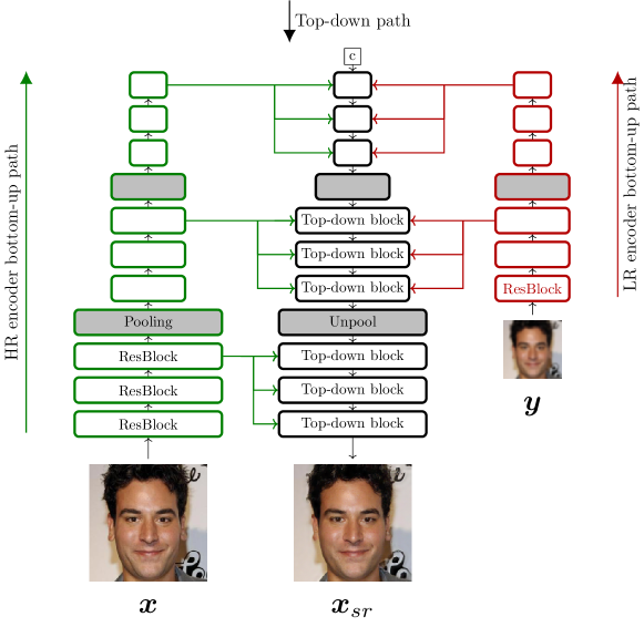
(a) CVDVAE architecture

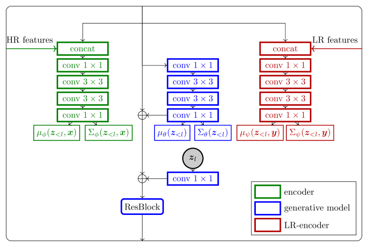
(b) Top-down block

Figure 2: Super-resolution model based on a pretrained VD-VAE model. (a) Given a pretrained VD-VAE network, composed of an encoder bottom-up network (in green), and a top-down network (in black), we train a LR encoder (in red) to encode low-resolution images in the latent space of VD-VAE. The LR-encoder has the same structure than VD-VAE encoder, with a bottom-up path that extracts multiscale features, and a top-down path merged with VD-VAE top-down path. (b) In each block of the top-down path, we add branch for the LR encoder (in red) to infer the statistics of $q_{\psi}\left(\bm{z}_{l}|\bm{z}_{<l},\bm{y}\right)$.

3 SUPER-RESOLUTION WITH HVAE

Problem formulation In this section we describe our super-resolution method based on a pretrained HVAE model. We assume that the LR image $\bm{y}\in\mathbb{R}^{3\times\frac{H}{s}\times\frac{W}{s}}$, and its associated HR image $\bm{x}\in\mathbb{R}^{3\times H\times W}$ are related by a linear degradation model:

$$\bm{y}=(k*\bm{x})\downarrow_{s},$$ (7)

where $k$ is a low-pass filter and $(u)\downarrow_{s}$ is defined as the subsampling operation with downsampling factor $s$. Our goal is to sample from the posterior distribution of the inverse problem:

$$p(\bm{x}|\bm{y})\propto p(\bm{y}|\bm{x})p(\bm{x}).$$ (8)

In (8), the likelihood $p(\bm{y}|\bm{x})$ can be deduced from the degradation model (7). On the other hand, the prior model $p(\bm{x})$ needs to be specified by the user. Deep generative models such as GANs, VAE or diffusion models can be used to model the prior on high-resolution images. In the following, we propose to parameterize $p(\bm{x})$ with a hierarchical variational autoencoder. Given a pretrained HVAE prior $p_{\theta}\left(\bm{x}\right)$, the ideal super-resolution model is:

$$p_{\theta}\left(\bm{x}|\bm{y}\right)=\int p_{\theta}\left(\bm{x}|\bm{y},\bm{z}\right)p_{\theta}\left(\bm{z}|\bm{y}\right)d\bm{z},$$ (9)

where probability laws correspond to the conditional of the augmented model $p_{\theta}\left(\bm{z},\bm{x},\bm{y}\right):=p_{\theta}\left(\bm{z}\right)p_{\theta}\left(\bm{x}|\bm{z}\right)p(\bm{y}|\bm{x})$. Since we do not have acces to $p_{\theta}\left(\bm{x}|\bm{y},\bm{z}\right)$ and $p_{\theta}\left(\bm{z}|\bm{y}\right)$, we can not directly sample from (9). However, we will see in the following part that we can efficiently approximate this model by making use of the structure of the HVAE hierarchical latent representation and of the its pretrained encoder.

Super-resolution model It has been observed in several works that the low-frequency information of images generated by HVAE model where mostly controlled by the low-resolution latent variable, at the beginning of the hierarchy [42, 4, 14]. Preliminary experiments, detailed in appendix A validate those previous observations. Hence, for a large enough number of latent groups $k$, samples from $p_{\theta}\left(\bm{x}|\bm{x}_{<k}\right)$ share the same low-frequency information. As a consequence, all the samples from $p_{\theta}\left(\bm{x}|\bm{x}_{<k}\right)$ are consistent to a LR image $\bm{y}$ (up to a small error). This motivates us to define the following super-resolution model:

$$p_{SR}\left(\bm{x}|\bm{y}\right)=\int p_{\theta}\left(\bm{x}|\bm{z}_{<k}\right)q_{\psi}\left(\bm{z}_{<k}|\bm{y}\right)d\bm{z},$$ (10)

where $q_{\psi}\left(\bm{z}|\bm{y}\right)$ is a stochastic low-resolution encoder, trained to encode the low-resolution latent groups. By definition of the super-resolution model (10), we can sample from $p_{SR}\left(\bm{x}|\bm{y}\right)$ by sequentially sampling $\bm{z}_{<k}\sim q_{\psi}\left(\bm{z}_{<k}|\bm{y}\right)$ and $\bm{x}\sim p_{\theta}\left(\bm{x}|\bm{z}_{<k}\right)$.

Hierarchical low-resolution encoder We set the LR encoder to have a hierarchical structure:

$$q_{\psi}\left(\bm{z}_{<k}|\bm{y}\right)=q_{\psi}\left(\bm{z}_{0}|\bm{y}\right)\prod_{l=1}^{k}q_{\psi}\left(\bm{z}_{l}|\bm{z}_{<l},\bm{y}\right),$$ (11)

with Gaussian conditional distributions:

$$\begin{cases}q_{\psi}\left(\bm{z}_{0}|\bm{y}\right)&=\mathcal{N}\left(\bm{z}_{0};\mu_{\psi,0}(\bm{y}),\Sigma_{\psi,0}(\bm{y})\right)\\ q_{\psi}\left(\bm{z}_{l}|\bm{z}_{<l},\bm{y}\right)&=\mathcal{N}\left(\bm{z}_{l};\mu_{\psi,l}(\bm{z}_{<l},\bm{y}),\Sigma_{\psi,l}(\bm{z}_{<l},\bm{y})\right).\\ \end{cases}$$ (12)

We implement the LR encoder with the same architecture as VD-VAE original (HR) encoder, but with a limited number of blocks due to reduced number of latent variable to be predicted (Figure 2). Only the parameters of the low-resolution encoder (in red in Figure 2) are trained, while the shared parameters (in blue in Figure 2) are set to the value of the corresponding parameters in the pretrained VD-VAE generative model, and remain frozen during training.

Training We keep the weights of the HVAE decoder $p_{\theta}\left(\bm{x}|\bm{z}\right)$, so that the only trainable weights of our super-resolution model (10) are the weights of the LR encoder $\psi$. Given a joint training distribution of HR-LR image pairs $p_{\mathcal{D}}\left(\bm{x},\bm{y}\right)$, the LR encoder is trained to match the available ”high-resolution” HVAE encoder $q_{\phi}\left(\bm{z}_{<k}|\bm{x}\right)$ on the associated HR images, by minimizing the Kullback-Leibler (KL) divergence:

$$\mathcal{L}(\psi)=\mathbb{E}_{p_{\mathcal{D}}\left(\bm{x},\bm{y}\right)}\left[KL\left(q_{\phi}\left(\bm{z}_{<k}|\bm{x}\right)||q_{\psi}\left(\bm{z}_{<k}|\bm{y}\right)\right)\right].$$ (13)

The criterion (13) was introduced by [13], who demonstrated that minimizing (13) is equivalent to maximizing a lower-bound of the super-resolution conditional log-likelihood on the training dataset, and that under additional assumptions on the pretrained HVAE model, one can reach optimal performance by only training the low-resolution encoder $q_{\psi}\left(\bm{z}_{<k}|\bm{y}\right)$. In practice, the KL divergence within the training criterion (13) can be decomposed into a sum of KL divergence on each latent subgroup:

$$\begin{split}&KL\left(q_{\phi}\left(\bm{z}_{<k}|\bm{x}\right)||q_{\psi}\left(\bm{z}_{<k}|\bm{y}\right)\right)=KL\left(q_{\phi}\left(\bm{z}_{0}|\bm{x}\right)||q_{\psi}\left(\bm{z}_{0}|\bm{y}\right)\right)\\ &+\mathbb{E}_{q_{\phi}\left(\bm{z}_{<k}|\bm{x}\right)}\left[\sum_{l=1}^{k}KL\left(q_{\phi}\left(\bm{z}_{l}|\bm{z}_{<l},\bm{x}\right)||q_{\psi}\left(\bm{z}_{l}|\bm{z}_{<l},\bm{y}\right)\right)\right].\end{split}$$ (14)

Since each conditional law involved in (14) is Gaussian, each KL term can be computed in closed-form. In practice the covariance matrices $\Sigma_{\phi,l}(\bm{z}_{<l},\bm{x})$ and $\Sigma_{\psi,l}(\bm{z}_{<l},\bm{y})$ are constrained to be diagonal, so that the KL can be computed efficiently.

4 EXPERIMENTS

4.1 Experimental settings

Dataset and upscaling factors

We test our super-resolution method CVDVAE on the FFHQ dataset [19], with images of resolution $256\times 256$. We experiment on 2 upscaling factors: $\times 4$ ($64\times 64\rightarrow 256\times 256$) and $\times 8$ ($32\times 32\rightarrow 256\times 256$). The low resolution images are initially downscaled by applying an antialiasing kernel followed by a bicubic interpolation.

Compared methods We compare CVDVAE with a conditional normalizing flow (HCFlow) [25], a conditional diffusion model (SR3) [38], and a method that add guidance to a non-conditional diffusion model at inference (DPS) [7]. We retrain HCFlow on FFHQ256 using the official implementation. For DPS, we also reuse the official implementation with the available pretrained model, which was trained on FFHQ. For SR3, since no official implementation is available, we used an open-source (non-official) implementation [17], and we trained a model on FFHQ. When training SR3, we found that a color shift [10] was responsible for important reconstruction errors. To compensate this weakness of the method, we project the super-resolved image on the space of consistent solutions at inference as proposed in [2]. For fair comparison, we retrained both HCFlow and SR3 with the same computational budget as for our low-resolution encoder. For HCFlow and CVDVAE, we set the temperature of the latent variables at $\tau=0.8$ during sampling.

Evaluating a diverse SR method Due to the ill-posedness of the problem, evaluating a diverse super-resolution model based solely on the distortion to the ground truth is not satisfactory. Indeed, there exist many solutions that are both realistic and consistent with the LR input while being far from the ground truth. Thus, in order to evaluate the super-resolution model, we provide a series of metrics that evaluate different expected characteristics of a diverse super-resolution model, such as the consistency of the solution, the diversity of the samples and the general visual quality. It should be noted that those metrics are not necessarily correlated: a model could generate diverse solutions, that are not consistent or realistic, or, on the opposite, it could provide solutions that are realistic and consistent but with a low diversity. Thus, to evaluate a diverse super-resolution model, it is necessary to consider these three different aspects together: diversity, consistency and visual quality.

Evaluation metrics The general quality of the super-resolved images is evaluated using the blind Image quality metric BRISQUE [32]. Consistency with the LR input is measured via peak Signal-to-Noise Ratio (PSNR, denoted as LR-PSNR in Tables 1 and 2). Furthermore, to evaluate the diversity of the super-resolution, we compute the Average Pairwise distance between different samples coming from the same LR input (denoted as APD in Tables 1 and 2), both at the pixel level, using the mean square error (MSE) between samples (considering pixel intensity value between 0 and 1), and at a perceptual level using the LPIPS similarity criteria [44]. For one LR input, the average pairwise distance is computed as the average distance between all the possible pairs of images in a set of 5 super-resolved samples. The reported APD in Tables 1 and 2 corresponds to the mean value of the single image APD over 500 LR inputs in the test set. We measure the distortion of the super-resolved samples with respect to the ground truth HR image in terms of PSNR, structural similarity (SSIM) [43] and LPIPS, as it is common in the super-resolution literature. All numbers reported correspond to the metric mean value on a subset of 1000 images from FFHQ256 test set.

4.2 Results

Quantitative evaluation

Table 1: Comparison of diverse SR methods face super-resolution. Best result is in bold, second best is underlined.

The quantitative results presented in Table 1 indicate that CVDVAE provides a good trade-off between the different evaluated metrics. Indeed, it obtains the second best results in terms of distortion and visual quality, and the second or third best results in terms of diversity. CVDVAE is also one of the fastest methods, along with HCFlow. HCFlow provides the best results for distortion metrics as it explicitly penalizes bad reconstruction in its training loss. Similar to CVDVAE, its application is fast, as it requires only one network evaluation to produce a super-resolved image. However, HCFlow lacks high-level diversity (as measured by the LPIPS average pairwise distance), compared with the concurrent methods. We postulate that this lack of diversity is due to the relative lack of expressiveness of normalizing flows architecture compared to the convolutional architectures used by diffusion and HVAE models. Our method, along with DPS, produces the best results in terms of visual quality as measured by the BRISQUE metric, illustrating the benefit of using a pretrained unconditional generative model. The computational cost of DPS is nevertheless significantly higher than the ones of CVDVAE and HCFlow, as DPS requires $1000$ steps of network evaluations (and backpropagation through the denoiser) to produce one super-resolved sample. Finally, SR3 performances are inferior to the compared methods. We used the same computational budget (48 hours on 4 GPUs) for training the SR3 models than our CVDVAE and HCFlow. This computational budget is significantly lower than the one reported in the SR3 paper [38] ($\approx 4$ days on 64 TPUv3 chip), and we expect that training the SR3 model for more epochs would improve its performance. Like DPS, SR3 is slower than our method as it requires 2000 network evaluations to produce one super-resolved image; although, unlike DPS, SR3 does not require to backpropagate through the score-network.

Qualitative evaluation Visual comparisons of super-resolved samples from the different evaluated methods are provided in Figures 3 and 4. CVDVAE is able to produce diverse textures as illustrated by the facial hair variation in Figure 3 or the hair variation in 4. CVDVAE appears to produce super-resolved samples with higher semantic diversity, in terms of textures (hairs, skin), in line with the higher perceptual diversity measured in the quantitative evaluation.

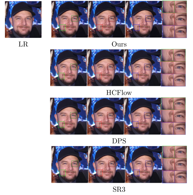
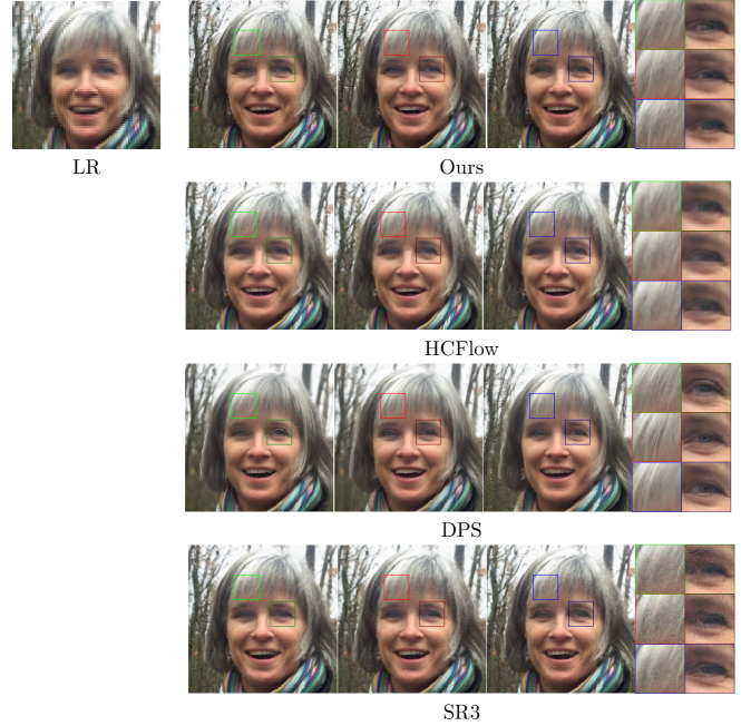
Figure 3: Samples from different diverse SR methods ($\times 4$)

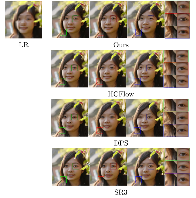
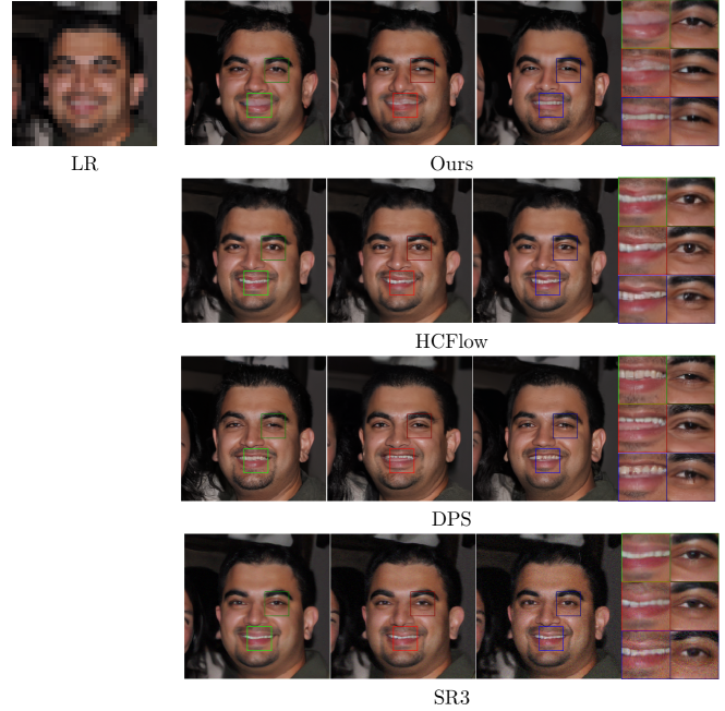
Figure 4: Samples from different diverse SR methods ($\times 8$)

Temperature control As for the unconditionnal HVAE models, CVDVAE offers the possibility to control the conditional generation via the temperature of the latent variable distributions [42, 4]. The temperature parameter $\tau$ controls the variance of the Gaussian latent distributions. In order to assess the behavior of the model on both low and high temperature regime, we evaluate our method on 2 temperatures ($\tau\in\{0.1,0.8\}$). Quantitative results in Table 2 show that reducing the temperature leads to a solution closer to the ground truth in terms of low-levels distortion metrics (PSNR and the SSIM), while using a higher temperature helps to improve the perceptual similarity (LPIPS) with the ground-truth, as well as the general perceptual quality of the generated HR images and the diversity of the samples. On Figure 5, we display CVDVAE’s samples at different temperatures $\tau$. The sampling temperature correlates with the perceptual smoothness of the super-resolved sample, a higher sampling temperature inducing images with sharper details.

Table 2: Effect of the sampling temperature $\tau$ on CVDVAE super-resolution results.

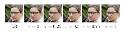
Figure 5: Effect of the sampling temperature $\tau$ on the super-resolved result. Increasing the temperature yields image with more high-frequency details.

5 RELATED WORKS

Super-resolution with pre-trained generative models

A large number of methods were designed to solve imaging inverse problems such as image super-resolution by using pretrained deep generative models (DGM) as a prior. This includes methods relying on generative adversarial networks (GAN) [31, 29, 33, 9, 8, 34], variational autoencoders [30, 12, 35] and denoising diffusion models [6, 7, 20, 40]. However, those approaches are computationally expensive as they require an iterative sampling or optimization procedure which require many network evaluation. On the other hand, our approach enables fast inference (one network evaluation), at the cost of reduced flexibility (due to the need of training a task-specific encoder). The idea of training an encoder to map a degraded image in the latent space of a generative network was previously exploited in the context of image inpainting with HVAE [13], and super-resolution with a GAN prior [3, 36].

Diverse super-resolution with conditional generative models

Although it is possible to sample from the posterior $p(\bm{x}|\bm{y})$ by using an unconditionnal deep generative models, those methods are restricted to specific dataset for which pretrained models are available. On generic natural images, the state of the art methods rely on conditional generative models, directly trained to model the posterior $p(\bm{x}|\bm{y})$ [27, 28]. Those methods include conditional normalizing flows [26, 25], conditional GAN [2], conditional VAE [11, 45, 5] and conditional denoising diffusion models [24, 38].

6 CONCLUSIONS

In this work we presented CVDVAE, a method that realizes an efficient sampling from the posterior of a super-resolution problem, by combining a low-resolution image encoder with a pretrained VD-VAE generative model. CVDVAE showed promising results on face super-resolution, on par with state-of-the-art diverse SR methods, providing semantically diverse and high-quality samples. Our results illustrate the ability of conditional hierarchical generative models to perform complex image-to-image tasks.

Our results are in line with many works that illustrates the benefits of using HVAE models for downstream applications [14, 1, 35]. One drawback of our approach is its limitation to dataset for which pretrained HVAE models are available, such as human faces or low-resolution ImageNet. However, we postulate that HVAE models have not yet reached their limits, and, by adapting design features from current SOTA deep generative models [37, 18] (architectural improvement, longer training, larger dataset), HVAE models could significantly improve their performance and expreessiveness, and generalize on much diverse datasets.

Appendix A Low-frequency information in VD-VAE latent represention

Average low-resolution pairwise distance between samples

We propose to evaluate which latent variables encode the low-frequency information within VD-VAE generative model. We measure how close the image generated by the conditional models $p_{\theta}\left(\bm{x}|\bm{z}_{<k}\right)$ are with each other, when they are downsampled with different downscaling factors. Without loss of generality, we consider the root mean square error (RMSE) as a measure of distance between samples. Thus, we estimate:

$$U_{k}^{s}:=\mathbb{E}_{p_{\theta}\left(\bm{z}_{<k}\right)}\mathbb{E}_{p_{\theta}\left(\bm{x}|\bm{z}_{<k}\right)}\mathbb{E}_{p_{\theta}\left(\bm{\tilde{x}}|\bm{z}_{<k}\right)}\left[\frac{1}{\sqrt{m}}\|H_{s}\bm{x}-H_{s}\bm{\tilde{x}}\|_{2}\right],$$ (15)

the average low-resolution pairwise distance of the generative model $p_{\theta}\left(\bm{x}|\bm{z}_{<k}\right)$, when samples are downsampled by a factor $s$. $U_{k}^{s}$ measures to what extent images sampled from $p_{\theta}\left(\bm{x}|\bm{z}_{<k}\right)$ differ from each other when they are downsampled.

Estimating $U_{k}^{s}$ We compute an estimations of the average sample low-resolution pairwise distance $U_{k}^{s}$ (15) with ancestral Monte-Carlo sampling. We sample $50$ different full latent codes $\bm{z}^{(i)}$ from the prior:

$$\bm{z}^{(i)}\sim p_{\theta}\left(\bm{z}\right).$$ (16)

For each latent code $\bm{z}^{(i)}$ and each number of fixed groups $k$, $5$ we sample five images:

$$\bm{x}^{(i,k,l)}\sim p_{\theta}\left(\bm{x}|\bm{z}_{<k}^{(i)}\right).$$ (17)

The average sample pairwise distance estimation is then computed as:

$$\hat{U_{k}^{s}}=\sum_{i=1}^{50}\sum_{1\leq l<m\leq 5}\frac{1}{\sqrt{m}}\|H_{s}\bm{x}^{(i,k,l)}-H_{s}\bm{x}^{(i,k,m)}\|_{2},$$ (18)

where $H_{s}$ is the downsampling operator associated to the downscaling factor $s$.

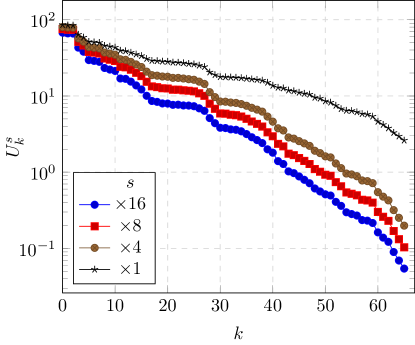
Figure 6: Average low-resolution pairwise distance, $U_{k}^{s}$ (15) between samples from the conditional generative model $p_{\theta}\left(\bm{x}|\bm{z}_{<k}\right)$ of VD-VAE, for downscaling factors $s=1,4,8,16$. Image with pixel values in $[0,255]$.

Low-resolution consistency of VD-VAE samples

In Figure 6 we estimate the value of $U_{k}^{s}$ for different downsampling factors. Results illustrate that, as the number of fixed groups $k$ increases, the generated images get more similar. Furthermore, for a given number of fixed groups $k$, the low-resolution pairwise distance decreases as the downsampling factor $s$ increases, indicating that there is more variation in the HR samples than in their LR counterparts. The gap between the average sample pairwise distance in high resolution ($s=1$), and low-resolution ($s\in\{4,8,16\}$) gets larger as the number of fixed groups $k$ increases, indicating that fixing a large number of groups $k$ yields samples that are close at low-resolution but different at high-resolution. The average low-resolution pairwise distance $U_{k}^{s}$ gets closer to zero as $k$ increases. While there is no value of $k$ such that $U_{k}^{s}=0$, we argue that for a large enough value of $k$, $U_{k}^{s}$ becomes negligible compared to the pixel intensity range (0-255), for instance $U_{60}^{4}<0.5$. Those results show that the downsampling of any image synthesized from the conditional generative model $p_{\theta}\left(\bm{x}|\bm{z}_{<k}\right)$ are consistent with one low-resolution image $\bm{y}$ with a certain precision inversely proportional to $k$.

References

- [1] S. Agarwal, G. Hope, A. Younis, and E. B. Sudderth. A decoder suffices for query-adaptive variational inference. In The 39th Conference on Uncertainty in Artificial Intelligence, 2023.
- [2] Y. Bahat and T. Michaeli. Explorable super resolution. In the IEEE/CVF Conference on Computer Vision and Pattern Recognition, pages 2716–2725, 2020.
- [3] K. C. Chan, X. Wang, X. Xu, J. Gu, and C. C. Loy. Glean: Generative latent bank for large-factor image super-resolution. In IEEE/CVF conference on computer vision and pattern recognition, pages 14245–14254, 2021.
- [4] R. Child. Very deep vaes generalize autoregressive models and can outperform them on images. arXiv preprint arXiv:12011.10650, 2021.
- [5] D. Chira, I. Haralampiev, O. Winther, A. Dittadi, and V. Liévin. Image super-resolution with deep variational autoencoders, 2022.
- [6] J. Choi, S. Kim, Y. Jeong, Y. Gwon, and S. Yoon. Ilvr: Conditioning method for denoising diffusion probabilistic models. arXiv preprint arXiv:2108.02938, 2021.
- [7] H. Chung, J. Kim, M. T. Mccann, M. L. Klasky, and J. C. Ye. Diffusion posterior sampling for general noisy inverse problems. In The Eleventh International Conference on Learning Representations, 2022.
- [8] G. Daras, Y. Dagan, A. Dimakis, and C. Daskalakis. Score-guided intermediate level optimization: Fast langevin mixing for inverse problems. In International Conference on Machine Learning, pages 4722–4753. PMLR, 2022.
- [9] G. Daras, J. Dean, A. Jalal, and A. Dimakis. Intermediate layer optimization for inverse problems using deep generative models. In International Conference on Machine Learning, pages 2421–2432. PMLR, 2021.
- [10] K. Deck and T. Bischoff. Easing color shifts in score-based diffusion models. arXiv preprint arXiv:2306.15832, 2023.
- [11] I. Gatopoulos, M. Stol, and J. M. Tomczak. Super-resolution variational auto-encoders. arXiv preprint arXiv:2006.05218, 2020.
- [12] M. González, A. Almansa, and P. Tan. Solving inverse problems by joint posterior maximization with autoencoding prior, 2021.
- [13] W. Harvey, S. Naderiparizi, and F. Wood. Conditional image generation by conditioning variational auto-encoders. In International Conference on Learning Representations, 2022.
- [14] J. D. Havtorn, J. Frellsen, S. Hauberg, and L. Maaløe. Hierarchical vaes know what they don’t know. In International Conference on Machine Learning, pages 4117–4128. PMLR, 2021.
- [15] L. Hazami, R. Mama, and R. Thurairatnam. Efficient-vdvae: Less is more, 2022.
- [16] J. Ho, A. Jain, and P. Abbeel. Denoising diffusion probabilistic models. Advances in Neural Information Processing Systems, 33:6840–6851, 2020.
- [17] L. Jiang. Image super-resolution via iterative refinement. https://github.com/Janspiry/Image-Super-Resolution-via-Iterative-Refinement, 2022.
- [18] M. Kang, J.-Y. Zhu, R. Zhang, J. Park, E. Shechtman, S. Paris, and T. Park. Scaling up gans for text-to-image synthesis. In IEEE/CVF Conference on Computer Vision and Pattern Recognition, pages 10124–10134, 2023.
- [19] T. Karras, S. Laine, and T. Aila. A style-based generator architecture for generative adversarial networks. In IEEE/CVF conference on computer vision and pattern recognition, pages 4401–4410, 2019.
- [20] B. Kawar, M. Elad, S. Ermon, and J. Song. Denoising diffusion restoration models. arXiv preprint arXiv:2201.11793, 2022.
- [21] D. P. Kingma, T. Salimans, R. Jozefowicz, X. Chen, I. Sutskever, and M. Welling. Improved variational inference with inverse autoregressive flow. Advances in neural information processing systems, 29, 2016.
- [22] D. P. Kingma and M. Welling. Auto-encoding variational bayes. arXiv preprint arXiv:1312.6114, 2013.
- [23] D. C. Lepcha, B. Goyal, A. Dogra, and V. Goyal. Image super-resolution: A comprehensive review, recent trends, challenges and applications. Information Fusion, 2022.
- [24] H. Li, Y. Yang, M. Chang, S. Chen, H. Feng, Z. Xu, Q. Li, and Y. Chen. Srdiff: Single image super-resolution with diffusion probabilistic models. Neurocomputing, 479:47–59, 2022.
- [25] J. Liang, A. Lugmayr, K. Zhang, M. Danelljan, L. Van Gool, and R. Timofte. Hierarchical conditional flow: A unified framework for image super-resolution and image rescaling. In IEEE/CVF International Conference on Computer Vision, pages 4076–4085, 2021.
- [26] A. Lugmayr, M. Danelljan, L. V. Gool, and R. Timofte. Srflow: Learning the super-resolution space with normalizing flow. In European conference on computer vision, pages 715–732. Springer, 2020.
- [27] A. Lugmayr, M. Danelljan, and R. Timofte. Ntire 2021 learning the super-resolution space challenge. In IEEE/CVF Conference on Computer Vision and Pattern Recognition, pages 596–612, 2021.
- [28] A. Lugmayr, M. Danelljan, R. Timofte, K.-w. Kim, Y. Kim, J.-y. Lee, Z. Li, J. Pan, D. Shim, K.-U. Song, et al. Ntire 2022 challenge on learning the super-resolution space. In IEEE/CVF Conference on Computer Vision and Pattern Recognition, pages 786–797, 2022.
- [29] R. V. Marinescu, D. Moyer, and P. Golland. Bayesian image reconstruction using deep generative models. arXiv preprint arXiv:2012.04567, 2020.
- [30] P.-A. Mattei and J. Frellsen. Leveraging the exact likelihood of deep latent variable models. Advances in Neural Information Processing Systems, 31, 2018.
- [31] S. Menon, A. Damian, S. Hu, N. Ravi, and C. Rudin. Pulse: Self-supervised photo upsampling via latent space exploration of generative models. In IEEE/CVF conference on computer vision and pattern recognition, pages 2437–2445, 2020.
- [32] A. Mittal, A. K. Moorthy, and A. C. Bovik. No-reference image quality assessment in the spatial domain. IEEE Transactions on image processing, 21(12):4695–4708, 2012.
- [33] X. Pan, X. Zhan, B. Dai, D. Lin, C. C. Loy, and P. Luo. Exploiting deep generative prior for versatile image restoration and manipulation. IEEE Transactions on Pattern Analysis and Machine Intelligence, 44(11):7474–7489, 2021.
- [34] Y. Poirier-Ginter and J.-F. Lalonde. Robust unsupervised stylegan image restoration. In IEEE/CVF Conference on Computer Vision and Pattern Recognition, pages 22292–22301, 2023.
- [35] J. Prost, A. Houdard, A. Almansa, and N. Papadakis. Inverse problem regularization with hierarchical variational autoencoders. In IEEE/CVF International Conference on Computer Vision (ICCV), pages 22894–22905, 2023.
- [36] E. Richardson, Y. Alaluf, O. Patashnik, Y. Nitzan, Y. Azar, S. Shapiro, and D. Cohen-Or. Encoding in style: a stylegan encoder for image-to-image translation. In IEEE/CVF conference on computer vision and pattern recognition, pages 2287–2296, 2021.
- [37] R. Rombach, A. Blattmann, D. Lorenz, P. Esser, and B. Ommer. High-resolution image synthesis with latent diffusion models. In IEEE/CVF conference on computer vision and pattern recognition, pages 10684–10695, 2022.
- [38] C. Saharia, J. Ho, W. Chan, T. Salimans, D. J. Fleet, and M. Norouzi. Image super-resolution via iterative refinement. arXiv preprint arXiv:2104.07636, 2021.
- [39] C. K. Sønderby, T. Raiko, L. Maalø e, S. r. K. Sø nderby, and O. Winther. How to train deep variational autoencoders and probabilistic ladder networks. In Advances in Neural Information Processing Systems, volume 29, 2016.
- [40] J. Song, A. Vahdat, M. Mardani, and J. Kautz. Pseudoinverse-Guided Diffusion Models for Inverse Problems. In (ICLR) International Conference on Learning Representations, 2023.
- [41] Y. Song, J. Sohl-Dickstein, D. P. Kingma, A. Kumar, S. Ermon, and B. Poole. Score-based generative modeling through stochastic differential equations. In International Conference on Learning Representations, 2021.
- [42] A. Vahdat and J. Kautz. Nvae: A deep hierarchical variational autoencoder. arXiv preprint arXiv:2007.03898, 2020.
- [43] Z. Wang, A. C. Bovik, H. R. Sheikh, and E. P. Simoncelli. Image quality assessment: from error visibility to structural similarity. IEEE transactions on image processing, 13(4):600–612, 2004.
- [44] R. Zhang, P. Isola, A. A. Efros, E. Shechtman, and O. Wang. The unreasonable effectiveness of deep features as a perceptual metric. In IEEE Conference on Computer Vision and Pattern Recognition, pages 586–595, 2018.
- [45] H. Zhou, C. Huang, S. Gao, and X. Zhuang. Vspsr: Explorable super-resolution via variational sparse representation. In IEEE/CVF Conference on Computer Vision and Pattern Recognition, pages 373–381, 2021.