Efficient visual object representation using a biologically plausible spike-latency code and winner-take-all inhibition

Abstract

Deep neural networks have surpassed human performance in key visual challenges such as object recognition, but require a large amount of energy, computation, and memory. In contrast, spiking neural networks (SNNs)have the potential to improve both the efficiency and biological plausibility of object recognition systems. Here we present a SNN model that uses spike-latency coding and winner-take-all inhibition (WTA-I)to efficiently represent visual stimuli from the Fashion MNIST dataset. Stimuli were preprocessed with center-surround receptive fields and then fed to a layer of spiking neurons whose synaptic weights were updated using spike-timing-dependent-plasticity (STDP). We investigate how the quality of the represented objects changes under different WTA-I schemes and demonstrate that a network of 150 spiking neurons can efficiently represent objects with as little as 40 spikes.

1 Introduction

Deep convolutional neural networks (DCNNs) have been extremely successful in a wide range of computer vision applications, rivaling or exceeding human benchmark performance in key visual challenges such as object recognition [7]. However, state-of-the-art DCNNs require too much energy, computation, and memory to be deployed on most computing devices and embedded systems [5]. In contrast, the brain is masterful at representing real-world objects with a cascade of reflexive, largely feedforward computations [4] that rapidly unfold over time [3] and rely on an extremely sparse, efficient neural code (see [1] for a recent review). For example, faces are processed in localized patches within inferotemporal cortex (IT), where cells detect distinct constellations of face parts (e.g., eyes, noses, mouths), and whole faces can be recognized by taking a linear combination of neuronal activity across IT [1].

Figure 1: Network architecture. Images from the Fashion MNIST dataset were convolved with ON and OFF center-surround kernels to simulate responses in the lateral geniculate nucleus (LGN). LGN responses were converted to spike latencies and fed to a spiking neural network (SNN)with plastic synapses implementing spike-timing-dependent-plasticity (STDP)and winner-take-all inhibition (WTA-I). The propagated LGN spikes contributed to an increase in the membrane potential of V1 neurons until one of the V1 membrane potentials reached threshold, resulting in a postsynaptic spike and inhibition of all other V1 neurons until the next iteration. The synaptic weights were updated using an unsupervised STDP rule. This allowed us to represent objects using the $\approx 40$ most active V1 neurons.

In recent years, spiking neural networks (SNNs) have emerged as a promising approach to improving the efficiency and biological plausibility of neural networks such DCNN, due to their potential for low power consumption, fast inference, event-driven processing, and asynchronous operation. Studying how object recognition may be implemented using biologically plausible learning rules in SNNs may not only further our understanding of the brain, but also lead to new efficient artificial vision systems.

Here we present a SNN model that uses spike-latency encoding [2] and winner-take-all inhibition (WTA-I) [8] to efficiently represent stimuli from the Fashion MNIST dataset [10]. We show that efficient object representations can be learned with spike-timing-dependent-plasticity (STDP) [6], an unsupervised learning rule that relies on sparsely encoded visual information among local neurons. In addition, we investigate how the quality of the represented objects changes under different WTA-I schemes. Remarkably, our network is able to represent objects with as little as 150 spiking neurons and at most 40 spikes.

2 Methods

2.1 Network architecture

The network architecture of our model is shown in Figure 1. Inspired by [2], our network consisted of an input layer corresponding to a simplified model of the lateral geniculate nucleus (LGN), followed by a layer of spiking neurons whose synaptic weights were updated using STDP. The LGN layer consisted of simulated firing-rate neurons with center-surround receptive fields, implemented using a 6x6 difference of Gaussian filter (see Figure 1, left). The LGN layer was fully connected to a layer of integrate-and-fire neurons, each unit characterized by a threshold and a membrane potential [2]. Thus, the LGN spikes contributed to an increase in the membrane potential of V1 neurons, until one of the V1 membrane potentials reached threshold, resulting in a postsynaptic spike. The membrane potential $E_{n}(t)$ of the $n^{th}$ V1 neuron at time $t$ within the iteration was represented as:

where $t_{m}$ was the spiking time of the $m$-th LGN neuron, ${H}$ was the Heaviside or unit step function, and $\theta$ was the threshold of the V1 neurons (assumed to be a constant for the entire population). The expression $\min\{t\mid\max E_{n}(t)\geq\theta\}$ denoted the timing of the first spike in the V1 layer. Membrane potentials were calculated up to this time point, after which a WTA-I scheme [8] was triggered and all membrane potentials were reset to zero. In this scheme, the most frequently firing neuron exerted the strongest inhibition on its competitors and thereby stopped them from firing until the end of the iteration.

2.2 Spike-latency code

Following [2], we converted the LGN activity maps to first-spike relative latencies using a simple inverse operation: $y=1/x$, where $x$ was the LGN input and $y$ was the assigned spike-time latency [9]. In this way, we ensured that the most active units fired first, while units with lower activity fired later or not at all.

2.3 Spike-timing dependent plasticity

The weights of plastic synapses connecting LGN and V1 were updated using STDP, which is an unsupervised learning rule that modifies synaptic strength, $w$, as a function of the relative timing of pre- and postsynaptic spikes, $\Delta t$ [6]. Long-term potentiation (LTP) ($\Delta{t}>0$) and long-term depression (LTD) ($\Delta{t}\leq 0$) were driven by their respective learning rates $\alpha^{+}$ and $\alpha^{-}$, leading to a weight change ($\Delta w$):

$$\Delta{w}=\begin{cases}-\alpha^{-}\cdot w^{\mu^{-}}\cdot K(\Delta{t},\tau_{-}),\Delta{t}\leq 0\\ \alpha^{+}\cdot(1-w)^{\mu^{+}}\cdot K(\Delta{t},\tau_{+}),\Delta{t}>0,\end{cases}$$ (2)

where $\alpha^{+}=5\times 10^{-3}$ and $\alpha^{-}=3.75\times 10^{-3}$, $K(\Delta{t},\tau)=e^{-|\Delta{t}|/\tau}$ was a temporal windowing filter, and $\mu^{+}=0.65$ and $\mu^{-}=0.05)$ were constants $\in[0,1]$ that defined the nonlinearity of the LTP and LTD process, respectively. In this implementation, computation speed greatly increased by making the windowing filter $K$ infinitely wide (equivalent to assuming $\tau_{\pm}\to\infty$, or $K=1$) [6].

A ratio $\alpha^{+}/\alpha^{-}=4/3$ was chosen based on previous experiments that demonstrated network stability [9]. The threshold of the V1 neurons was fixed through trial and error at $\theta=20$. This value was unmodified for all experiments.

Initial weight values were sampled from a random uniform distribution between 0 and 1. After each iteration, the synaptic weights for the first V1 neuron to fire were updated using STDP (Equation 2), and the membrane potentials of all the other neurons in the V1 population were reset to zero. The STDP rule was active only during the training phase. STDP has the effect of concentrating high synaptic weights on afferents that systematically fire early, thereby decreasing postsynaptic spike latencies for these connections.

2.4 Winner-take-all inhibition

We used a hard WTA-I scheme such that, if any V1 neuron fired during a certain iteration, it simultaneously prevented other neurons from firing until the next sample [8]. This scheme computes a function WTA-I _n$:\mathbb{R}^{n}\rightarrow\{0,1\}^{n}$ whose output $\langle y_{1},...,y_{n}\rangle$ = WTA-I _n ($x_{1}$,…, $x_{n}$) satisfied:

$$y_{i}=\begin{cases}1,\,\,\,\,$if $x_{i}$ $>$ $x_{j}$ for all $j\neq i$ $\\ 0,\,\,\,\,$if $x_{j}$ $>$ $x_{i}$ for some $j\neq i$ $.\end{cases}$$ (3)

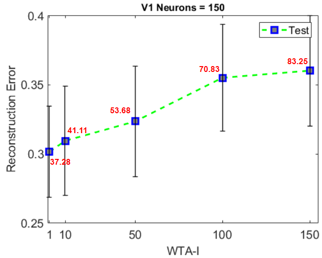
For a given set of $n$ different inputs $x_{1},...,x_{n}$, a hard WTA-I scheme would thus yield a single output $y_{i}$ with value $1$ (corresponding to the neuron that received the largest input $x_{i}$), whereas all other neurons would be silent. We also implemented various soft WTA-I schemes to investigate how the quality of the represented objects changes. The soft WTA-I schemes consisted of 10, 50, 100 and 150 (i.e., all V1 neurons) neurons firing during a certain iteration, while all other neurons were silenced (see Figure 5).

Original

LGN

OR

Original

LGN

OR

Figure 2: Examples of object representation. First and fourth columns: Fashion MNIST samples. Second and fifth columns: LGN activity maps (after preprocessing). Third and sixth columns: Object representation (OR) using a hard WTA-I scheme with 150 V1 neurons, which aimed to reconstruct the LGN activity maps.

2.5 Dataset

We assessed the ability of our SNN network to represent visual stimuli using the Fashion MNIST database [10]. The Fashion-MNIST dataset comprises $28\times 28$ grayscale images of 70,000 fashion products from 10 categories, with 7,000 images per category. To train the network, we randomly selected 1,000 training images and 200 test images.

2.6 Stimulus reconstruction

The post-convergence receptive field $\xi_{j}$ of the $i$-th V1 neuron was estimated as follows:

$$\xi_{j}\approx\sum\limits_{j\in{LGN}}w_{ij}\psi_{j},$$ (4)

where $\psi_{j}$ was the receptive field of the $j$-th LGN afferent, and $w_{ij}$ was the weight of the synapse connecting the $j$-th afferent to the $i$-th V1 neuron.

Stimuli $k$ were then linearly reconstructed from the V1 population activity:

$$OR_{k}=\sum\limits_{j\in{V1}}r_{kj}\xi_{j},$$ (5)

where $r_{kj}$ was the response of the $j$-th V1 neuron to the $k$-th image and $\xi_{j}$ was its receptive field.

3 Results

Figure 3: Reconstruction error for the training and test sets using different V1 neurons for a hard WTA-I scheme (WTA-I = 1). Number of spikes needed to optimally represent an object during the test phase is given in red.

LGN

V1 = 10
0.3308

V1 = 50
0.3229

V1 = 100
0.3076

V1 = 150
0.2964

V1 = 200
0.2951

V1 = 250
0.3007

Figure 4: Representation of a shoe using a population of V1 neurons (ranging from 10 to 250 neurons). The number below each image indicates the reconstruction error for that particular image.

3.1 Object representation using hard WTA-I

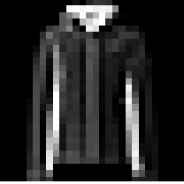
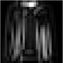
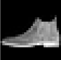
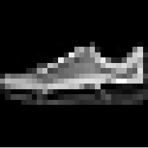
Example object reconstructions obtained after training with a hard WTA-I scheme (i.e., where only one neuron was active for each training image) are shown in Figure 2. Here, every spiking neuron became selective for a particular object feature (example receptive fields learned by STDP are shown in Figure 1), so that after training a whole object could be represented by a linear combination of V1 neurons (Equation 5).

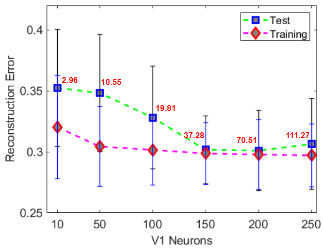
Figure 3 shows the reconstruction error after training for both the training and the test sets using different V1 neurons for a hard WTA-I scheme. Reconstruction error for an image $k$ was calculated as the mean square error between the LGN activity map ($\mathrm{LGN}_{k}$) and $\mathrm{OR}_{k}$. Figure 3 reports the mean and standard deviation of all reconstruction errors across the train and test sets, respectively. We found that the reconstruction error for the training set decreased with an increasing number of V1 neurons. On the other hand, the reconstruction error of the test set went through a minimum (at roughly 150 V1 neurons), which is consistent with the bias-variance dilemma [1]. In addition, the number of spikes needed to represent an object increased with the number of V1 neurons, nearly doubling from 37.28 spikes at 150 neurons to 70.51 spikes at 200 neurons. Increasing the V1 population beyond 150 neurons did therefore not lead to any visible benefits in reconstruction error (Figure 4), but required many more spikes to represent an object.

3.2 Object representation using soft WTA-I schemes

We also tested object representation using various soft WTA-I schemes, where we varied the number of V1 neurons allowed to be active for each training image. Figure 5 shows the reconstruction error on the test set across the range of possible WTA-I schemes, ranging from hard (where for every image only one neuron was active) to soft (where all neurons (150) were active). We found that the softer the WTA-I scheme, the higher the reconstruction error and the number of spikes needed to represent an object. The reason for this became evident when we visualized the resulting object representations (Figure 6). WTA-I schemes where at most 10 neurons were allowed to be active where instrumental in maintaining competition among neurons. In the absence of a strong WTA-I scheme, multiple neurons ended up learning similar visual features, which resulted in poor object reconstructions (right half of Figure 6).

4 Conclusion

We have shown that a network of spiking neurons relying on biologically plausible learning rules and coding schemes can efficiently represent objects from the Fashion MNIST dataset with as little as 40 spikes. WTA-I schemes were essential for enforcing competition among neurons, which led to sparser object representations and lower reconstruction errors. A future extension of the model might focus on deeper architectures and more challenging visual stimuli.

Figure 5: Reconstruction error in the test phase as a function of the number of spikes included in the STDP algorithm (WTA-I) for 150 V1 neurons. Number of spikes needed to optimally represent an object during the test phase is given in red.

LGN

WTA-I-1
0.2964

WTA-I-10
0.3007

WTA-I-50
0.3164

WTA-I-100
0.3415

WTA-I-150
0.3508

Figure 6: Representation of a shoe using different WTA-I schemes, where between 1 (WTA-I 1) and 150 (WTA-I 150) neurons were active for each training sample. The number below each image indicates the reconstruction error for that particular image.

References

- [1] M Beyeler, EL Rounds, KD Carlson, N Dutt, and JL Krichmar. Neural correlates of sparse coding and dimensionality reduction. PLoS Computational Biology, 15(6), 2019.
- [2] T Chauhan, T Masquelier, A Montlibert, and BR Cottereau. Emergence of binocular disparity selectivity through Hebbian learning. Journal of Neuroscience, 38(44):9563–9578, 2018.
- [3] RM Cichy, D Pantazis, and A Oliva. Similarity-Based Fusion of MEG and fMRI Reveals Spatio-Temporal Dynamics in Human Cortex During Visual Object Recognition. Cerebral Cortex, 26(8):3563–3579, 07 2016.
- [4] JJ DiCarlo, D Zoccolan, and NC Rust. How does the brain solve visual object recognition? Neuron, 73(3):415–434, 2012.
- [5] A Goel, C Tung, Y-H Lu, and GK Thiruvathukal. A survey of methods for low-power deep learning and computer vision. In 2020 IEEE 6th World Forum on Internet of Things (WF-IoT), pages 1–6. IEEE, 2020.
- [6] R Gütig, R Aharonov, S Rotter, and H Sompolinsky. Learning Input Correlations through Nonlinear Temporally Asymmetric Hebbian Plasticity. Journal of Neuroscience, 23(9):3697–3714, May 2003. Publisher: Society for Neuroscience Section: ARTICLE.
- [7] K He, X Zhang, S Ren, and J Sun. Delving deep into rectifiers: Surpassing human-level performance on imagenet classification. In 2015 IEEE International Conference on Computer Vision (ICCV), pages 1026–1034, 2015.
- [8] W Maass. On the computational power of winner-take-all. Neural Computation, 12(11):2519–2535, 2000.
- [9] T Masquelier and SJ Thorpe. Unsupervised learning of visual features through spike timing dependent plasticity. PLoS Computational Biology, 3(2):e31, 2007.
- [10] H Xiao, K Rasul, and R Vollgraf. Fashion-MNIST: A novel image dataset for benchmarking machine learning algorithms. arXiv preprint arXiv:1708.07747, 2017.