User Localization using RF Sensing: A Performance comparison between LIS and mmWave Radars

Abstract

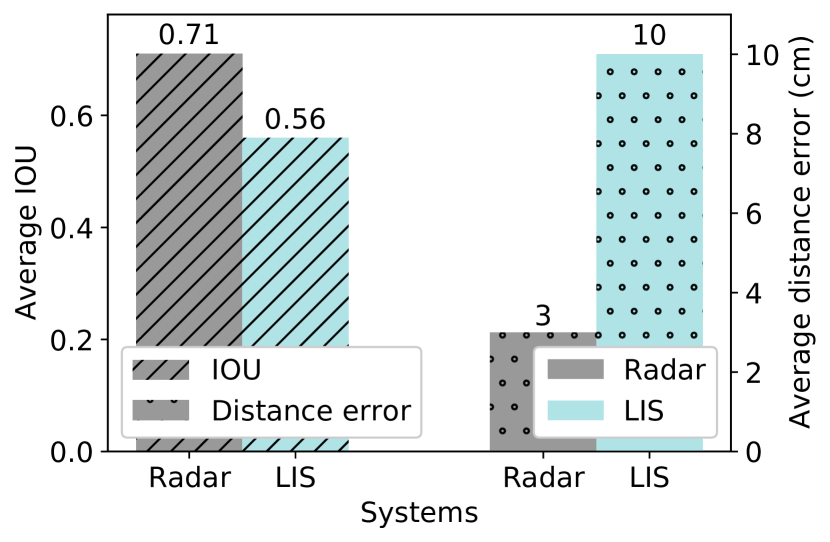
Since electromagnetic signals are omnipresent, Radio Frequency (RF)-sensing has the potential to become a universal sensing mechanism with applications in localization, smart-home, retail, gesture recognition, intrusion detection, etc. Two emerging technologies in RF-sensing, namely sensing through Large Intelligent Surfaces (LISs) and mmWave Frequency-Modulated Continuous-Wave (FMCW) radars, have been successfully applied to a wide range of applications. In this work, we compare LIS and mmWave radars for localization in real-world and simulated environments. In our experiments, the mmWave radar achieves 0.71 Intersection Over Union (IOU) and 3cm error for bounding boxes, while LIS has 0.56 IOU and 10cm distance error. Although the radar outperforms the LIS in terms of accuracy, LIS features additional applications in communication in addition to sensing scenarios.

I Introduction

Recently, with the advance of robots, remote controlled and autonomous vehicles (UAVs, vehicles), localization and positioning has become a key support capability. RGB cameras [1], lidars [2], and Radio Frequency (RF) sensors [3] are common approaches used for localization. Lidars are capable of providing an accurate 3D model of an environment. Their performance is affected by weather conditions though [4]. This is similar for RGB cameras, which also have a reduced performance in challenging lighting conditions [5]. RF-based sensors and Large Intelligent Surface (LIS) are resilient to lighting and weather conditions[5].

Figure 1: Schematic comparison of the two systems (a) LIS-based, (b) radar-based

Wireless sensing is becoming integrated into future communication systems [6]. Specifically, with the increasing count of antennas added to Base Stations (BSs), researchers have exploited first Multiple-Input-Multiple-Output (MIMO), then massive MIMO, and now LIS, a continuous electromagnetic surface, comprising a large number of tightly spaced small antenna elements, capable of transmitting and receiving electromagnetic signals. LIS are capable to support communication as well as sensing [7]. Likewise, mmWave radars have been widely used in many sensing applications from gesture recognition [8, 9, 10] to localization [3].

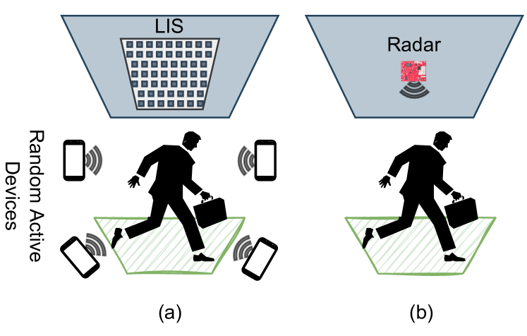
In this work, we compare, for the first time in the literature, these two technologies to solve a sensing-based localization task as it is shown in Fig. 1. We perform experimental measurements using an Frequency-Modulated Continuous-Wave (FMCW) radar, namely IWR1443, operating in the 77-81 GHz RF-band. Since no LIS prototypes exist yet in the market, we perform a comprehensive simulation based on ray-tracing, mimicking the experimental environment. In particular, we will reconstruct the radio map of the propagation environment using an indoor LIS deployment in the ceiling, as also described in [11].

II System Models and Problem Formulation

In this section, we discuss the configurations of the two systems. The LIS system is implemented in a simulation environment, while the radar system has a real-world test-bed.

II-A LIS System Model

We consider an indoor setting in which $D_{a}$ active devices are present. The devices transmit for communication. Sensing with the LIS is then subsequently performed by piggybacking these signals.

A LIS of $A$ antenna elements is placed at the room’s ceiling. We assume an ideal LIS made up of isotropic antennas. Therefore, physical effects such as mutual coupling are neglected. The sensing task is to create a radio map that captures a person in the environment by superimposing the received signals from each of the $d\in D_{a}$ elements at each of the $A$ LIS components. The superposed complex baseband signal received at the LIS is given by

$$\mathbf{y}=\sum_{d=1}^{D_{a}}\mathbf{h_{d}}x_{d}+\mathbf{n}.$$ (1)

Here, $x_{d}$ is the transmitted symbol from device $d$ (without loss of generality, we consider $x_{d}=1$), $\mathbf{h_{d}}\in\mathbb{C}^{N\times 1}$ is the channel vector from a specific position of device $d$ to each antenna-element, and $\mathbf{n}\sim\mathcal{CN}_{N}(\mathbf{0},\sigma^{2}\mathbf{I}_{N})$ is the noise vector. For simplicity, we consider narowband transmissions and this removes the effect of frequency selectivity.

The large physical dimensions of the LIS, compared with the distance from the transmitters to the ceiling, lead to a spherical-wave propagation condition. The spherical-wave channel coefficient $h_{sp,a}$ at the $a$-th element from an arbitrary active device transmission is proportional to [12]

$$h_{sp,a}\ \propto\ \frac{1}{d_{a}}e^{-j\frac{2\pi}{\lambda}d_{a}},$$ (2)

where $d_{a}$ denotes the distance between the active device and the $a$-th antenna. To compute the radio map, we can derive a Matched Filter (MF) such that [11]

$$\mathbf{y_{mf}}=\mathbf{h_{sp}}\ast\mathbf{y}.$$ (3)

In eq 3, $\ast$ denotes the convolution operator, $\mathbf{h_{sp}}\in\mathbb{C}^{N_{f}\times 1}$ is the expected spherical pattern (steering vector) for $N_{f}$ antennas LIS deployment on (2), $\mathbf{y}$ is the received signal from (1) and $\mathbf{y_{mf}}\in\mathbb{C}^{A\times 1}$ is the filtered output that represents the radio map. We zero-pad $\mathbf{y}$ such that we guarantee $\mathbf{y_{mf}}\in\mathbb{C}^{A\times 1}$ dimension to perform the convolution. To obtain the radio map, we compute the energy at the output of the MF. In this way, we are measuring the energy of the signals reflected from the target. In order to design the filter, we assume knowledge of the frequency $f$ and the distance $d$ (the $z$ coordinate, since the LIS is deployed at the ceiling) between the transmitter and the LIS . Figure 2 shows the detection of the target on the LIS processed radio map.

Figure 2: A radio map obtained for an $M=118\times 118$ antenna elements $\frac{\lambda}{2}$ spaced LIS in a noiseless scenario with $D_{a}=5$ active devices by using a MF design for $f=3.5$ GHz, $d=3.2$ m and $N_{f}=100\times 100$ antenna elements $\frac{\lambda}{2}$ spaced.

II-A1 Simulated scenario

We perform simulations via ray tracing [13] in a $4.7\times 4.7\times 3.2$ m simulated area. We deploy a LIS with $118\times 118$ elements separated by $\lambda/2$. The $D_{a}$ active devices transmit narrowband signals of 20 dBm at 3.5 GHz and they are randomly deployed in the space $(x,y,z)$. The distance from which the MF is calibrated is $d=3.2$, as we set a kernel for the procedure such that it scans the entire height of the room. The human is modeled as a rectangle of dimensions 0.3x0.5x1.83 m (reasonable human dimensions obtained from [14]) with conductivity $s=1.44$ S/m, relative permittivity $\varepsilon=38.1$ and relative permeability $\mu=1$ [15]. To be fair with the experimental setup, the positions of the passive human $(x,y,z=1.83)$ m are randomly selected in a circle of radius 2.5 m.

II-A2 Received signal and noise modeling

From the ray-tracing simulation, the received signal in (1) is obtained as the complex electric field arriving at the $n$-th antenna element, $\widetilde{E}_{a}$, which can be regarded as the superposition of each ray path $r\in N_{r}$ from every $d\in D_{a}$ device, i.e.,

$$\widetilde{E}_{a}=\sum_{d=1}^{D_{a}}\sum_{r=1}^{N_{r}}\widetilde{E}_{a,r,d}=\sum_{d=1}^{D_{a}}\sum_{r=1}^{N_{r}}E_{a,r,d}e^{j\phi_{a,r,d}}.$$ (4)

The complex signal at the output of the $n$-th element is therefore given by

$$y_{a}=\sqrt{\frac{\lambda^{2}Z_{a}}{4\pi Z_{0}}}\widetilde{E}_{a}+n_{a}.$$ (5)

Here, $\lambda$ is the wavelength, $Z_{0}=120\pi$ os the free space impedance and $Z_{n}$ is the antenna impedance. For simplicity, we consider $Z_{n}=1\,\forall\,n$. Finally, we define the average Signal-to-Noise Ratio (SNR), $\overline{\gamma}$, as

$$\overline{\gamma}\triangleq\frac{\lambda^{2}}{4\pi Z_{0}M\sigma^{2}}\displaystyle\sum_{a=1}^{A}|\widetilde{E}_{a}|^{2},$$ (6)

where $A$ denotes the number of antenna elements in the LIS.

II-B Radar System Model

Figure 3: (a) Overview structure of the radar-based localization system. The radar transforms the IQ samples into a point cloud through the radar processing pipeline. Then, the point cloud processing pipeline predicts a bounding box using as the localization output. (b) Overview structure of the LIS-based localization system. The LIS processes the reflected complex signal by applying the MF procedure to obtain the radio map. Then, the radio map processing part predicts a bounding box around the target user. The random $D_{a}$ active devices are piggybacked to perform the sensing.

We utilize the IWR1443 mmWave FMCW radar operating at 77GHz with 4GHz bandwidth. We further process the point cloud data generated by the radar to perform localization.

II-B1 Point Cloud Generation

The radar evaluation kit performs a four step processing pipeline to generate point cloud data from Analog to Digital Converter (ADC) data as shown in Fig. 3.a.

Range Fast Fourier Transform (FFT) (1D): A chirp signal, i.e. a sinusoidal signal with increasing frequency through time, is generated by the radar. Then the mixing operation produces an intermediate frequency signal using transmitted and reflected chirps. The range of the system is linearly proportional to the intermediate signal’s frequency, computed through FFT operations.

Doppler FFT (2D): The radial velocity of the target is proportional to the phase difference of multiple chirps at the range-FFT peak. To generate a peak at the velocity of target, a FFT is applied on the signal range (i.e., a 2D-FFT or a Doppler-FFT).

Constant False Alarm Rate (CFAR): For each virtual antenna, a pre-detection matrix is formed through summation of Doppler-FFT matrices. The CFAR algorithm [16] then filters the pre-deteciton matrix to produce peaks corresponding to targets.

Angle-FFT: For each target, an angle-FFT is applied on corresponding CFAR peaks across multiple Doppler-FFTs. Velocity-induced phase changes are Doppler-corrected before angle-FFT calculation.

II-B2 Point Cloud Processing

We follow a three-step point cloud processing tool-chain to localize the target.

Time Decay: We configured the radar to sample 33 point clouds per second. Since points in each frame are sparse ($\approx$ 5 per frame), we apply time decay to increase density. Empirically, a time-window of size 5 ($\approx$ 151 ms) is used to slide through time frames to increase the number of points in each frame.

Graph Generation: From the time-decayed point cloud, we then build a graph. Consider a point cloud $X=\{x_{1},...,x_{n}\}\subseteq\mathbb{R}^{F}$ where each point $x_{i}$ is represented by a feature set $\{f_{i}^{1},...,f_{i}^{F}\}$. A graph-K-Nearest Neighbor (KNN) algorithm is exploited to produce the KNN-graph $\mathcal{G}=\{X,\mathcal{E}\}$ where $\mathcal{E}\subseteq X\times X$ is the set of directed edges between each point and its nearest neighbours in the Euclidean space.

Graph Processing using Message Passing Neural Network (MPNN): Following a similar approach as [17], each node’s representation is updated using the proposed MPNN layer. In each layer, an aggregation function is applied to the representation of the node itself and to its neighbors’ features:

$$h_{i}^{0} =x_{i},$$ (7)

$$h_{i}^{l} =\underset{j:(i,j)\in\mathcal{E}}{\Gamma}(\Delta_{\theta}(h^{l-1}_{i},h^{l-1}_{j})),$$

in which, $h_{i}^{l}$ is point $i$’s representation in layer $l$, message function $\Delta_{\theta}:\mathbb{R}^{F}\times\mathbb{R}^{F}\rightarrow\mathbb{R}^{F^{\prime}}$ is a learnable function with parameters $\theta$ which is implemented using Multi Layer Perceptron (MLP), and $\Gamma$ is a channel-wise symmetric aggregation operator (e.g. $\Sigma$, max, or mean) applied on the messages of the edge emanating from each neighbor. To capture not only local but also global structures of the input point cloud, we use $\Delta_{\theta}(h_{i},h_{j})=\bar{\Delta}_{\theta}(h_{i},h_{j}-h_{i})$ meaning that for each edge, we concatenate the features of the incident node of the edge with the difference between the two nodes connected by the edge.

The details of the localization model is shown in Fig. 3. We empirically use the proposed layer in Eq.7, PointLoc, twice in the architecture of the model. Then we concatenate the output of the two layers followed by an MLP to achieve a vector representation of the input point cloud with length of 1024. Finally, after applying a few layers of MLP to extract fine-grained features, we use a linear layer with 4 neurons and without activation function to output the four dimensions of the bounding box. The loss function is Mean Squared Error (MSE).

II-C Main Assumptions

The main assumptions for both approaches are as follows. With respect to LIS, we assume that mutual coupling is ignored. It is commonly represented using a coupling matrix that takes into account the influence of nearby antennas [18] but the influence can be compensated after estimation, and hence does not affect any conclusion drawn. Radar and LIS have a Line-of-Sight (LOS) to the target. Also, to design the filter we need to assume a-priori the frequency $f$ and the distance from a transmitter to the LIS $d$. However, this last parameter is not a very strong assumption (cf. Section II-A1). We therefore set it to be the distance as if the transmitter were on the floor. This means that the transmitters can be at different distances and are not limited by the filter design.

The field of view of the radar is -55^∘ to +55^∘.

III Implementation and Evaluation

In this section, we explain the way we collected data in the real-world environment for the mmWave radar and simulation environment for LIS. Then, we elaborate on the model training process, evaluation metrics, and finally the localization performance comparison between the radar and the LIS.

III-A Dataset

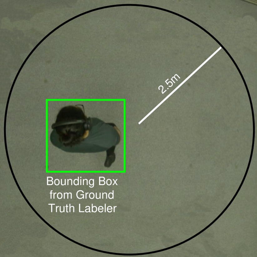
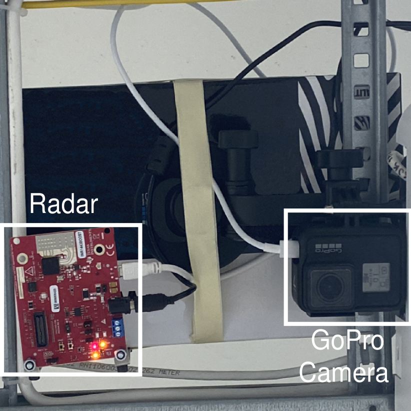
To collect the radar data (cf. Fig. 4(a)), we marked a circular area with 2.5m radius on the floor and asked participants to walk arbitrarily inside the circle. A IWR1443 radar and a GoPro camera were mounted in 3m height over the center of the circle record ground truth point cloud and video data (Fig. 4(b)). We labelled the video using the Ground Truth Labeler application. The radar data was labeled manually by matching the bounding boxes from the video with the point cloud data. Three subjects participated in the experiment and 15,000 samples have been collected. Training, validation and testing is performed following a 60/10/30 split.

For the LIS, we simulated the same circular area with 2.5m radius and simulated random positions of the target. The positions are processed by obtaining radio maps using $D_{a}=5$ active devices randomly deployed in the room. 15,000 samples were recorded.

(a)

(b)

Figure 4: (a) The experiment environment which is a circle with 2.5m radius marked on the ground. (b) An IWR1443 radar and a GoPro camera installed on the ceiling with 3m height.

III-B Radar Model Training Process

We used a computer with 32GB of RAM and an Nvidia GeForce 940MX GPU for training and inference. The model for the radar pipeline is implemented based on PyTorch and PyTorch Geometric [19] frameworks. An early stopping scheme with a patience of 100 epochs is exploited to prevent from over-fitting. In other words, if no improvement is observed on the validation set within the patience period, we stop the training process and save the best model.

MSE is used as the loss function to train the model, Adam Optimizer [20] with step-decay strategy to train the network:

$$L_{r}=L_{i}\cdot d_{r}^{\lfloor\frac{e}{e_{r}}\rfloor}.$$ (8)

Here, $L_{r}$ is the learning, $L_{i}$ is the initial value of the learning rate, $d_{r}$ is the drop rate after every $e_{r}$ epochs, $e$ is the current epoch and $\lfloor\cdot\rfloor$ is the floor operator. In our experiments $L_{i}$, $d_{r}$, and $e_{r}$ are $0.001$, $0.5$, and $20$, respectively.

III-C LIS Radio Map Based Localization

We process the radio map by obtaining the indices of the maximum peak value to infer the human position, i.e.

$$(x_{c},y_{c})=\arg\max_{xp,yp}|\mathbf{y_{mf}}|\times\Delta s,$$ (9)

In this equation, $x_{c}$ and $y_{c}$ denote the inferred position, $x_{p}$ and $y_{p}$ the position in the pixel domain and $\Delta s$ the antenna spacing.

III-D LIS Bounding Box Creation

As we are not using a learning algorithm, but want to compare LIS and radar systems, we compute manually a bounding box considering the center the inferred positions.

As we know the dimensions of our target (detailed in Section II-A1) we can compute a bounding box from the center position such that

$$(x_{min},y_{min})=(x_{c}-\frac{L}{2},y_{c}-\frac{W}{2}),$$ (10)

$$(x_{max},y_{max})=(x_{c}+\frac{L}{2},y_{c}+\frac{W}{2}),$$ (11)

with $L=0.5$ m and $W=0.3$ m (cf. Section II-A1).

III-E Evaluation Metric

To evaluate the performance of the models we use Intersection Over Union (IOU) and the Euclidean distance between the center of the ground truth bounding box and the predicted bounding box. The IOU is defined by:

$$\lx@glossaries@gls@link{acronym}{iou}{\leavevmode IOU}_{i}=\dfrac{|P_{i}\cap G_{i}|}{|P_{i}\cup G_{i}|},$$ (12)

where $P_{i}$ and $G_{i}$ are predicted and ground truth bounding boxes for sample $i$. We report the average IOU and Euclidean distance between the centers of the ground truth and the predicted bounding boxes on the test set for each of the approaches.

III-F Localization Comparison

Figure 5: Average IOU and distance error for radar and LIS

As shown in Fig. 5, the average IOU for the LIS in localization is 0.56 while the Radar it is 0.71. This result suggests that the radar is more accurate in estimating the bounding box for the target. We have a similar result for the average distance error of the bounding boxes. The radar outperforms the LIS with only 3cm in contrast to 10cm average error. These results suggest that mmWave radars are more accurate than LIS, but in scenarios where the accuracy of sensing can be compromised, LIS can provide simultaneous communication and sensing capabilities without a need for a third-party device. Also, there might be potential scenarios in which LIS would outperform the radar. For example, decreasing the inter-antenna spacing would lead to more accurate localization results for the LIS. However, we showed the common inter-antenna distance design ($\frac{\lambda}{2}$) to provide a close comparison to the radar.

IV Conclusion

So far, mmWave radars have been considered the standard de facto for indoor localization given their incredibly cheap components and localization accuracy. However, the breakthroughs in communications systems are leading to devices that can integrate both sensing and communications. LISs arise as a brand-new device which communications capabilities are expected to go beyond massive MIMO. However, their sensing functionality is still under investigation. In this paper, we have shown a comparison among LIS and mmWave radars in an indoor sensing-based localization task. Results show that LIS is not that different from mmWave radars in localization accuracy, with the advantage of leading to a new system that can integrate both sensing and communications. In most scenarios there is no need to have a very accurate localization, including but not limited to industrial localization systems or localizing users for beamforming. In those scenarios, LIS can also act as a sensing device providing communications and sensing capabilities at the same time.

References

- [1] K. Kononov, R. Lavrenov, L. Gavrilova, and T. Tsoy, “External rgb-d camera based mobile robot localization in gazebo environment with real-time filtering and smoothing techniques,” in Electromechanics and Robotics. Springer, 2022, pp. 223–234.
- [2] Y. Zhang, L. Wang, X. Jiang, Y. Zeng, and Y. Dai, “An efficient lidar-based localization method for self-driving cars in dynamic environments,” Robotica, vol. 40, no. 1, pp. 38–55, 2022.
- [3] S. Palipana, B. Pietropaoli, and D. Pesch, “Recent advances in rf-based passive device-free localisation for indoor applications,” Ad Hoc Networks, vol. 64, pp. 80–98, 2017.
- [4] Y. Li, Y. Liu, Y. Wang, Y. Lin, and W. Shen, “The millimeter-wave radar slam assisted by the rcs feature of the target and imu,” Sensors, vol. 20, no. 18, p. 5421, 2020.
- [5] S. Palipana, D. Salami, L. A. Leiva, and S. Sigg, “Pantomime: Mid-air gesture recognition with sparse millimeter-wave radar point clouds,” Proceedings of the ACM on IMWUT, vol. 5, no. 1, pp. 1–27, 2021.
- [6] M. Latva-aho and K. Leppänen, “Key drivers and research challenges for 6G ubiquitous wireless intelligence (white paper),” 6G Flagship research program, University of Oulu, Finland, 2019.
- [7] C. J. Vaca-Rubio, P. Ramirez-Espinosa, K. Kansanen, Z.-H. Tan, E. de Carvalho, and P. Popovski, “Assessing wireless sensing potential with large intelligent surfaces,” arXiv preprint arXiv:2011.08465, 2020.
- [8] D. Salami, R. Hasibi, S. Savazzi, T. Michoel, and S. Sigg, “Integrating sensing and communication in cellular networks via nr sidelink,” arXiv preprint arXiv:2109.07253, 2021.
- [9] D. Salami, R. Hasibi, S. Palipana, P. Popovski, T. Michoel, and S. Sigg, “Tesla-rapture: A lightweight gesture recognition system from mmwave radar sparse point clouds,” IEEE Transactions on Mobile Computing, 2022.
- [10] D. Salami and S. Sigg, “Zero-shot motion pattern recognition from 4d point-clouds,” in MLSP 2021. IEEE, 2021, pp. 1–6.
- [11] C. J. Vaca-Rubio, P. Ramirez-Espinosa, K. Kansanen, Z.-H. Tan, and E. de Carvalho, “Radio sensing with large intelligent surface for 6G,” arXiv preprint arXiv:2111.02783, 2021.
- [12] Z. Zhou, X. Gao, J. Fang, and Z. Chen, “Spherical wave channel and analysis for large linear array in los conditions,” in Globecom Workshops. IEEE, 2015, pp. 1–6.
- [13] Feko, altair engineering, inc. https://www.altairhyperworks.com/feko.
- [14] P. Potkány, M. Debnár, M. Hitka, and M. Gejdoš, “Requirements for the internal layout of wooden house from the point of view of ergonomics changes,” Zeszyty Naukowe. Quality. Production. Improvement, 2018.
- [15] P. S. Hall, Y. Hao, Y. I. Nechayev, A. Alomainy, C. C. Constantinou, C. Parini, M. R. Kamarudin, T. Z. Salim, D. T. Hee, R. Dubrovka et al., “Antennas and propagation for on-body communication systems,” IEEE Antennas and Propagation Magazine, vol. 49, no. 3, pp. 41–58, 2007.
- [16] M. A. Richards, J. Scheer, W. A. Holm, and W. L. Melvin, “Principles of modern radar,” 2010.
- [17] Y. Wang, Y. Sun, Z. Liu, S. E. Sarma, M. M. Bronstein, and J. M. Solomon, “Dynamic graph cnn for learning on point clouds,” Acm Transactions On Graphics (tog), vol. 38, no. 5, pp. 1–12, 2019.
- [18] T. Su and H. Ling, “On modeling mutual coupling in antenna arrays using the coupling matrix,” Microwave and Optical Technology Letters, vol. 28, no. 4, pp. 231–237, 2001.
- [19] M. Fey and J. E. Lenssen, “Fast graph representation learning with pytorch geometric,” arXiv preprint arXiv:1903.02428, 2019.
- [20] D. P. Kingma and J. Ba, “Adam: A method for stochastic optimization,” arXiv preprint arXiv:1412.6980, 2014.