Treatment Effects in Bunching Designs: The Impact of Mandatory Overtime Pay on Hours

Abstract

The 1938 Fair Labor Standards Act mandates overtime premium pay for most U.S. workers, but it has proven difficult to assess the policy’s impact on the labor market because the rule applies nationally and has varied little over time. I use the extent to which firms bunch workers at the overtime threshold of 40 hours in a week to estimate the rule’s effect on hours, drawing on data from individual workers’ weekly paychecks. To do so I generalize a popular identification strategy that exploits bunching at kink points in a decision-maker’s choice set. Making only nonparametric assumptions about preferences and heterogeneity, I show that the average causal response among bunchers to the policy switch at the kink is partially identified. The bounds indicate a relatively small elasticity of demand for weekly hours, suggesting that the overtime mandate has a discernible but limited impact on hours and employment.

1 Introduction

Many countries require premium pay for long work hours, in an effort to limit excessive work schedules and encourage hours to be spread over more workers. In the U.S., such regulation comes through the “time-and-a-half” rule of the Fair Labor Standards Act (FLSA): firms must pay a worker one and a half times their normal hourly wage for any hours worked in excess of 40 within a single week. Although many salaried workers are exempt, the time-and-a-half rule applies to a majority of the U.S. workforce, including nearly all of its over 80 million hourly workers. Workers in many industries average multiple overtime hours per week, making overtime the largest form of supplemental pay in the U.S. [29, 6].

Nevertheless, only a small literature has studied the effects of the FLSA overtime rule on the labor market. This stands in marked contrast to the large body of work on the minimum wage, which was also introduced at the federal level by the FLSA in 1938. A key reason for this gap is that the overtime rule has varied little since then: the policy has remained as time-and-a-half after 40 hours in a week, for now more than 80 years. Reforms to overtime policy have been rare and have focused on eligibility, leaving the central parameters of the rule unaffected. This lack of variation has afforded few opportunities to leverage research designs that exploit policy changes to identify causal effects, and remains as the Department of Labor mulls a major expansion to eligibility expected to be announced in late 2023 [52].

This paper assesses the effect of the FLSA overtime rule on hours of work, taking a new approach that makes use of variation within the rule itself. The policy introduces a sharp discontinuity in the marginal cost of a worker-hour—a convex “kink” in firms’ costs—which provides firms with an incentive to set workers’ hours exactly at 40. Optimizing behavior by firms predicts that the resulting mass of workers working 40 hours in a given week will be larger or smaller depending on how responsive firms are to the wage increase imposed by the time-and-a-half rule. Combining this observation with assumptions about the shape of the distribution of hours that would be chosen absent the FLSA, I use the bunching mass to identify the effect of the overtime rule on hours.

To do so, I develop a generalization of the “bunching design” identification strategy, which has previously used bunching at kinks in income tax liability to identify the elasticity of labor supply to the net-of-tax rate ([45, 18]). This paper provides new identification results under weakened bunching design assumptions likely suitable to a variety of empirical contexts, showing that the method can be useful for program-evaluation questions such as assessing the effect of the FLSA.

In income tax settings, the promise of the bunching design is to overcome endogeneity in the marginal tax rates that apply to different individuals, while requiring for identification only the cross-sectional distribution of income near a threshold between tax brackets. Analogously, my starting point in the overtime setting is to construct the distribution of weekly work hours. Administrative hours data at the weekly level has previously been unavailable, and studies of overtime in the U.S. have typically relied on self-reported integer hours from surveys such as the Current Population Survey. I instead obtain detailed data via individual paycheck records from a large payroll processing company. Among workers paid weekly, these paychecks report the exact number of hours that the worker was paid for in a given week, allowing me to construct the distribution of hours-of-pay without rounding or other sources of measurement error.

With these new data in hand, my goal is to translate features of the observed hours distribution into estimates of the overtime rule’s causal effect, under credible assumptions about how weekly working hours are determined. This requires moving beyond the standard bunching-design model popularized in public-finance applications, in which decision-makers have parametric “isoelastic” preferences and strong restrictions are placed on heterogeneity. In the overtime setting, I show that bunching is informative about firms (rather that workers) as the decision-maker, choosing the hours of each of their workers in a given week. Having established this, the identifying assumptions of the bunching design can be separated into two parts: i) assumptions about how individual agents (firms) would make choices given counterfactual choice sets—a choice model, and ii) assumptions about the distribution of heterogeneity in choices across observational units (paychecks).

As a first methodological contribution, I show that the class of choice models under which the bunching design can be used is considerably more general than the benchmark isoelastic model and its variants. In particular, I find that the method need not rest upon the researcher positing any explicit functional form for decision-makers’ (firms’) utility; rather, the main prediction about choice driving identification comes from convexity of preferences (e.g. weekly profits). Agents can furthermore have multiple underlying margins of choice which might be unobserved to the researcher, and preferences can vary flexibly by observational unit. While a non-parametric choice model has previously been considered by [8] to study identification in the bunching design, I extend to a general class of models and distill from this class a common implication about what is observable. My positive identification results then rest on a prediction about choices that remains broadly valid when the isoelastic utility model often employed is misspecified.

The generality of this approach is accomplished by defining the parameter of interest in terms of a pair of counterfactual choices rather than as a preference parameter from a parametric choice model, recasting the bunching design in the language of potential outcomes. In the overtime setting these potential outcomes correspond to: a) the number of hours the firm would choose for the worker this week if the worker’s normal wage rate applied to all of this week’s hours; and b) the number that the firm would choose if the worker’s overtime rate applied to all of this week’s hours. I show that choice from a kinked choice set can be fully characterized by this pair of counterfactuals: agents choose one or the other of them or they choose the location of the kink. Bunching at the kink directly identifies a feature of the joint distribution of the potential outcomes, allowing one to make statements about treatment effects purged of selection bias.

While generalizing the choice model underlying the bunching design, I also propose a new approach to weakening assumptions about heterogeneity required by the method. [9] emphasize that identification from bunching rests on assumptions regarding the distribution heterogeneity that cannot be directly verified in the data. In my formulation, such assumptions take the form of extrapolating the marginal distributions of each of the two potential outcomes, which are both observed in a censored manner. To perform this extrapolation I impose a natural nonparametric shape constraint— bi-log-concavity—on the distribution of each potential outcome. Bi-log-concavity nests many previously proposed distributional assumptions for bunching analyses, is in-part testable, and can be economically motivated in the case of hours. The restriction affords partial identification of a conditional average treatment effect among units located at the kink, a parameter I call the “buncher ATE”. In the overtime context, the buncher ATE yields an average wage elasticity of hours demand. While the buncher ATE represents a reduced form quantity, I leverage additional assumptions to use it for assessing the overall average effect of the FLSA.

My results supplement other partial identification approaches recently proposed for the bunching design. Notably, the bounds I derive for the buncher ATE are substantially narrowed by making extrapolation assumptions separately for each of two counterfactuals. By contrast, existing approaches operate by constraining the distribution of a single scalar heterogeneity parameter, a simplification afforded by the isoelastic choice model. In the context of that model, [3] and [9] obtain bounds on the elasticity when the researcher is willing to put an explicit limit on how sharply the density of heterogeneous choices can rise or fall. My approach based on bi-log-concavity avoids the need to choose any such tuning parameters, and is applicable in the general choice model.

I also show that the data in the bunching design are informative about counterfactual policies that change the location or “sharpness” of a kink. To do so, I extend a characterization of bunching from [8], and show that when combined with a general continuity equation [33] the result yields bounds on the derivative of bunching and mean hours with respect to policy parameters. I use this to evaluate proposed reforms to the FLSA: e.g. lowering the overtime threshold below 40 hours (e.g. the Thirty-Two Hour Workweek Act proposed in the U.S. House of Representatives in 2021), or increasing the premium pay factor from 1.5 to 2.

The empirical setting of overtime pay involves confronting two challenges that are not typical of existing bunching-design analyses. Firstly, 40 hours is not an “arbitrary” point and bunching there could arise in part from factors other than it being the location of the kink. I use two strategies to estimate the amount of bunching that would exist at 40 absent the FLSA, and deliver clean estimates of the rule’s effect. My preferred approach exploits the fact that when a worker makes use of paid-time-off hours these do not count towards that week’s overtime threshold, shifting the location of the kink week-to-week in a plausibly idiosyncratic way. A second feature of the overtime setting is that work hours may not be set unilaterally by one party: in principle either the firm or the worker could have control over a given worker’s schedule. I provide evidence that week-to-week variation in hours tends to be driven by firms, but show that even when bargaining weight between workers and firms is arbitrary and heterogeneous, bunching at 40 hours is informative about labor demand rather than supply.

Empirically, I find that the FLSA overtime rule does in fact reduce hours of work among hourly workers, despite the theoretical possibility that offsetting wage adjustments might eliminate any such effect [51]. My preferred estimate suggests that about one quarter of the bunching observed at 40 among hourly workers is due to the FLSA, and those working at least 40 hours work, on average, about 30 minutes less in a week than they would absent the time-and-a-half rule. Across specifications, I obtain estimates of the local wage elasticity of weekly hours demand near 40 hours in the range $-0.04$ to $-0.19$, indicating that firms are fairly resistant to changing hours to avoid overtime payments. A back-of-the-envelope calculation using these effects suggests that FLSA regulation creates about 700,000 jobs (relative to an estimated 100 million non-exempt workers), despite a reduction in total hours.

The structure of the paper is as follows. Section 2 lays out a motivating conceptual framework for work hours that relates my approach to existing literature on overtime. Section 3 introduces the payroll data I use in the empirical analysis. In Section 4 I develop the generalized bunching-design approach, with Appendix B expanding on some of the supporting formal results. Section 5 applies these results to estimate effect of the FLSA overtime rule on work hours, as well as the effects of proposed reforms to the FLSA. Section 6 discusses the empirical findings from the standpoint of policy objectives, and 7 concludes.

2 Conceptual framework

This section outlines a framework useful for reasoning about the determination of weekly work hours among hourly workers, which motivates the identification strategy of Section 4. Readers primarily interested in the bunching design may wish to skip directly to that section.

Given the time-and-a-half rule, total pay for a given worker in a particular week is a kinked function of the worker’s hours that week, as depicted in Figure 1. This is true provided that the worker’s hourly wage $w$ is fixed with respect to the choice of hours that week. Indeed, the data detailed in Section 3 reveal that hours tend to vary considerably between weeks for a given hourly worker, while workers’ wages change only infrequently. I propose to view this as a two stage-process. In a first step, workers are hired with an hourly wage set along with an “anticipated” number of weekly hours. Then, with that hourly wage fixed in the short-run, final scheduling of hours is controlled by the firm and varies by week given shocks to the firm’s demand for labor.

Figure 1: With a given worker’s straight-time wage fixed at $w$, labor costs as a function of hours have a convex kink at $40$ hours, given the overtime rule. Simple models of week-by-week hours choice (see Section 4.2) yield bunching when for some workers, the marginal product of an hour at 40 is between $w$ and $1.5w$.

Wages and anticipated hours set at hiring

We begin with the hiring stage, which pins down the worker’s wage. The hourly rate of pay $w$ that applies to the first 40 of a worker’s hours is referred to as their straight-time wage or simply straight wage. The following provides a benchmark model to endogenize such straight wages. This yields predictions about how wages may themselves be affected by the overtime rule, which will prove useful in our final evaluation of the FLSA. However, the basic bunching design strategy of Section 4 will only require that some straight-time wage is agreed upon and fixed in the short-run for each worker, as can be observed directly in the data.

Suppose that firms hire by posting an earnings-hours pair $(z,h)$, where $z$ is total weekly compensation offered to each worker, and $h$ is the number of hours of work per week advertised at the time of hiring. The firm faces a labor supply function $N(z,h)$ determined by workers’ preferences over the labor-leisure tradeoff, and makes a choice of $(z^{*},h^{*})$ given this labor supply function and their production technology. For simplicity, workers are here taken to be homogeneous in production, paid hourly, and all covered by the overtime rule.

While labor supply has above been viewed as a function over total compensation $z$ and hours, there is always a unique straight wage associated with a particular $(z,h)$ pair, such that $h$ hours of work yields earnings of $z$, given the FLSA overtime rule:

$$w_{s}(z,h):=\frac{z}{h+0.5\cdot\mathbbm{1}(h>40)(h-40)}$$ (1)

We can distinguish the two main views proposed in the literature regarding the effects of overtime policy by supposing that a worker’s straight-time wage is set according to Eq. (1), given values $z^{*}$ and $h^{*}$ that the firm and worker agree upon at the time of hiring. [51] calls these two views the fixed-job and the fixed-wage models of overtime.

The fixed-job view observes that for a generic smooth labor supply function $N(z,h)$ (and smooth revenue production function with respect to hours), the optimal job package $(z^{*},h^{*})$ for the firm to post will be the same as the optimal one absent the FLSA, as the hourly wage rate simply adjusts to fully neutralize the overtime premium. Suppose for the moment that workers in fact work exactly $h^{*}$ hours each week (abstracting away from any reasons for the firm to ever deviate from $h^{*}$ in a given week). Then the FLSA would have no effect on earnings, hours or employment, provided that $w_{s}(z^{*},h^{*})$ is above any applicable minimum wage [51].

On the fixed-wage view, the firm instead faces an exogenous straight-time wage when determining $(z^{*},h^{*})$. Versions of this idea are considered in [11], [44], [23], [27], [29] and [15]. This can be captured by a discontinuous labor supply function $N(z,h)$ that exhibits perfect competition on the quantity $w_{s}(z,h)$. I show in Appendix LABEL:app:hiringmodel that in this case $h^{*}$ and $z^{*}$ are pinned down by the concavity of production with respect to hours and the scale of fixed costs (e.g. training for each worker) that do not depend on hours. The fixed-wage job makes the clear prediction that the FLSA will cause a reduction in hours, and bunching at 40.

Existing work has investigated whether the fixed-job or fixed-wage model better accords with the observed joint distribution of hourly wages and hours [51, 1]. These papers find that wages do tend to be lower among jobs that have overtime pay provisions and more overtime hours, but by a magnitude smaller than would be predicted by the pure fixed job model. These estimates could be driven by selection however, e.g. of lower-skilled workers into covered jobs with longer hours. In Appendix E.3, I construct a new empirical test of Eq. (1) (at the level of individual paychecks), that is instead based on assuming that the conditional distribution of pay is smooth across 40 hours. I find that roughly one quarter of paychecks around 40 hours reflect the wage/hours relationship predicted by the fixed-job model.

This finding is consistent with a model in which hours remain flexible week-to-week, while straight-wages remain fairly static after being set initially according to Equation (1). In common with the fixed wage model, this two-stage framework allows for the possibility that the overtime rule affects hours, and predicts bunching at 40; however, this is driven by short-run rigidity in straight-wages, rather than by perfect competition as in previous fixed-wage approaches.

Dynamic adjustment to hours by week

After $(z^{*},h^{*})$ is set, there are many reasons to still expect week-to-week variation in the number of hours that a firm would desire from a given worker. If demand for the firm’s products is seasonal or volatile, it may not be worthwhile to hire additional workers only to reduce employment later. Similarly, productivity differences between workers may only become apparent to supervisors after those workers’ straight wages have been set, and vary by week.

Throughout Section 4, I maintain a strong version of the assumption that the firm—rather than the worker—chooses the final hours that I observe on a given paycheck. This simplification eases notation and emphasizes the intuition behind my identification strategy. Appendix C presents a generalization in which some fraction of workers choose their hours, along with intermediate cases in which the firm and worker bargain over hours each week. The results there show that if some workers have control of their final hours, the bunching-design strategy will only be informative about effects of the FLSA among workers whose final hours are chosen by the firm.

Available survey evidence suggests that this latter group is the dominant one: a relatively small share of workers report that they choose their own schedules. For example, the 2017-2018 Job Flexibilities and Work Schedules Supplement of the American Time Use Survey asks workers whether they have some input into their schedule, or whether their firm decides it. Only 17% report that they have some input. In a survey of firms, only 10% report that most of their employees have control over which shifts they work [40].

3 Data and descriptive patterns

The main dataset I use comes from a large payroll processing company. They provided anonymized paychecks for workers from a random sample of their employers, for all pay periods in 2016 and 2017. At the paycheck level, I observe the check date, straight wage, and amount of pay and hours corresponding to itemized pay types, including normal pay, overtime pay, sick pay, holiday pay, and paid time off. The data also include state and industry for each employer and for employees: age, tenure, gender, state of residence, pay frequency and salary if one is specified for them.

3.1 Sample description

I construct a final sample for analysis based on two desiderata: a) the ability to observe hours within a single week; and b) a focus on workers who are non-exempt from the FLSA overtime rule. For the purposes of a), I drop paychecks from workers who are not paid on a weekly basis (roughly half of the workers in the sample). To achieve b) I keep paychecks only from hourly workers, since nearly all workers who are paid hourly are subject to the overtime rule. I also drop any workers who have no variation in hours or never receive overtime pay during the study period. The final sample includes 630,217 paychecks for 12,488 workers across 566 firms. See Appendix E.1 for further details of the sample construction.

	(1)	(2)	(3)	(4)
	Estimation sample	Initial sample	CPS	NCS
Tenure (years)	3.21	2.81	6.34	.
Age (years)	37.15	35.89	39.58	.
Female	0.23	0.46	0.50	.
Weekly hours	38.92	27.28	36.31	35.70
Gets overtime	1.00	0.37	0.17	0.52
Straight-time wage	16.16	22.17	18.09	23.31
Weekly overtime hours	3.56	0.94	.	1.04
Number of workers in sample	12488	149459	63404	228773

Table 1: Comparison of the sample with representative surveys. Columns 1 and 2 average across periods within worker from the administrative payroll sample, and then present means across workers. Column 2 presents means of worker-level data from the Current Population Survey and Column 3 averages representative job-level data from the National Compensation Survey.

Table 1 shows how the sample compares to survey data that is constructed to be representative of the U.S. labor force. Column (1) reports means from the final sample used in estimation, while (2) reports means before sampling restrictions. Column (3) reports means from the Current Population Survey (CPS) for the same years 2016–2017, among individuals reporting hourly employment. The “gets overtime” variable for the CPS sample indicates that the worker usually receives overtime, tips, or commissions. Column (4) reports means for 2016–2017 from the National Compensation Survey (NCS), a representative establishment-level dataset accessed on a restricted basis from the Bureau of Labor Statistics. The NCS reports typical overtime worked at the quarterly level for each job in an establishment (drawn from firm administrative data when possible).

The sample I use is somewhat more male, earns lower straight-time wages, and works more overtime than a typical hourly worker in the U.S. Column (2) in Table 1 reveals that my sampling restrictions can explain why the estimation sample tilts male and has higher overtime hours than the workforce as a whole. The initial sample is fairly representative on both counts, while conditioning on workers paid weekly oversamples industries that have more men, longer hours, and lower pay. Appendix E compares the industry and regional distributions of the estimation sample to the CPS.

3.2 Hours and wages in the sample

I turn now to the main variables to be used in the analysis. Figure 2 reports the distribution of hours of work in the final sample of paychecks. The graphs indicate a large mass of individuals who were paid for exactly 40 hours that week, amounting to about 11.6% of the sample. Appendix Figure E.8 shows that overtime pay is present in nearly all weekly paychecks that report more than 40 hours, in line with the presumption that workers in the final sample are not FLSA-exempt.

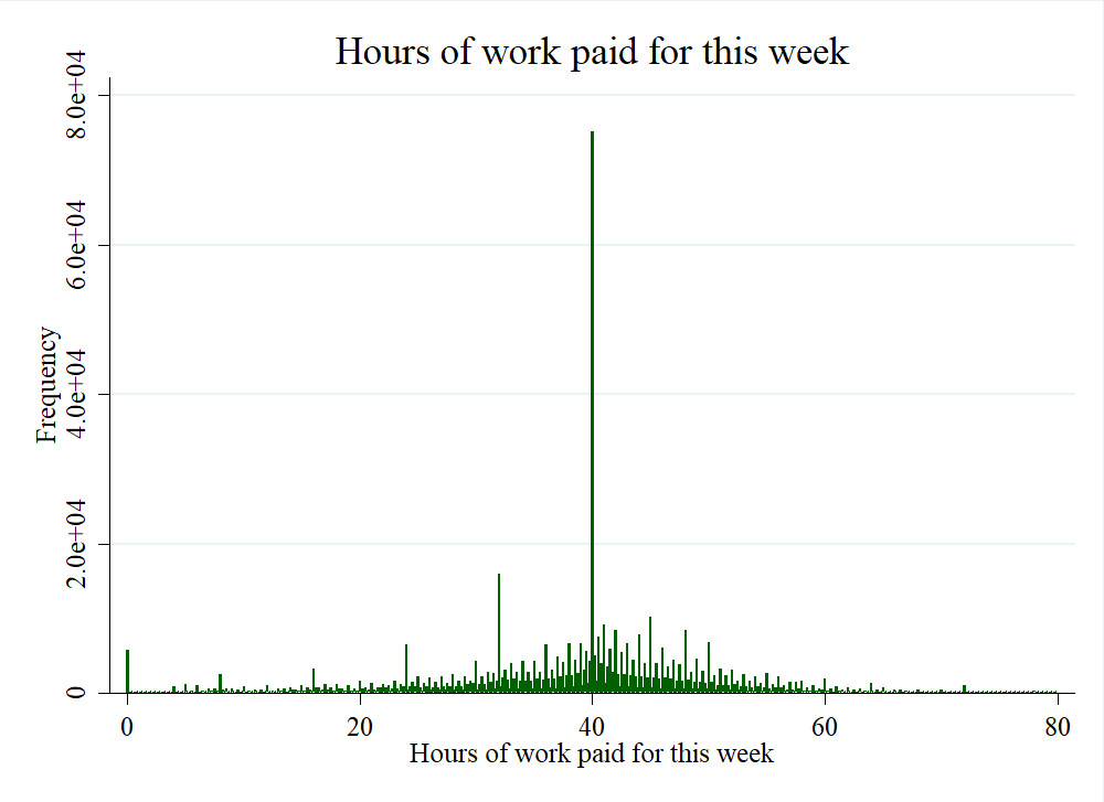
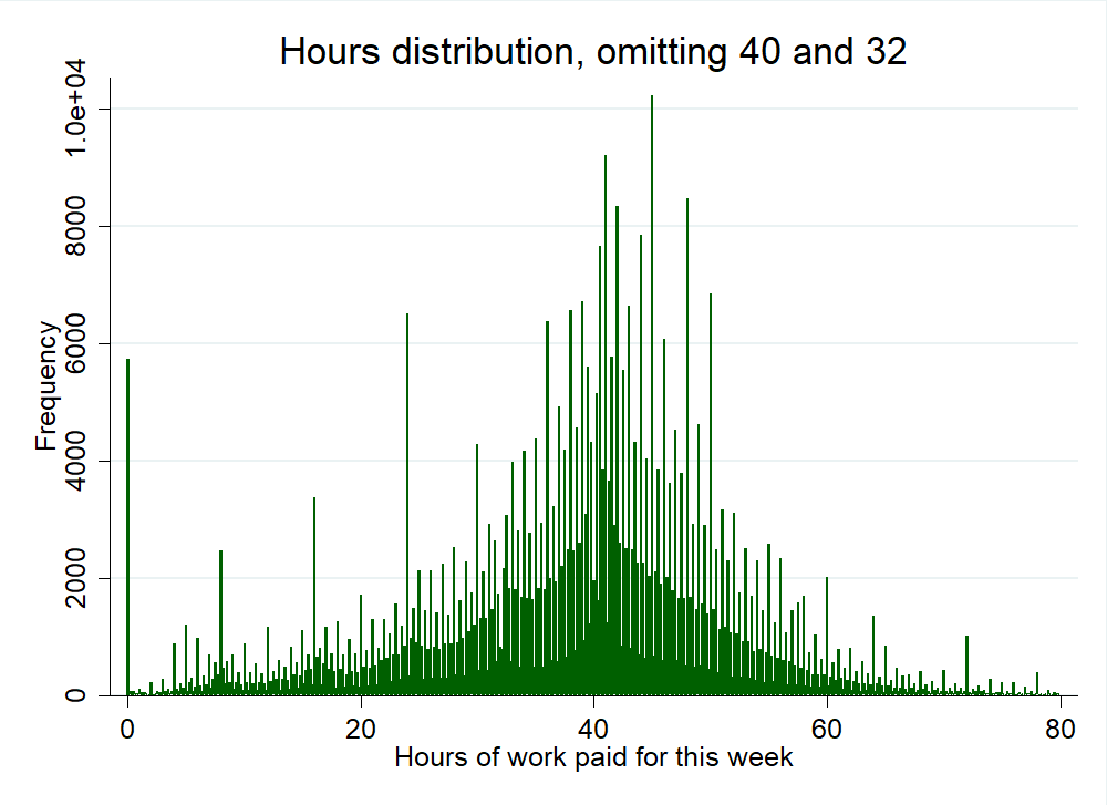
Figure 2: Empirical densities of hours worked pooling all paychecks in final estimation sample. Sample is restricted to hourly workers receiving overtime pay at some point (to ensure nearly all are non-exempt from FLSA, see text), and workers having hours variation. The right panel omits the points 40 and 32 to improve visibility elsewhere. Bins have a width of 1/8, below the granularity at which most firms record hours.

Table 2 documents that while the hours paid in 70% of all pay checks in the final estimation sample differ from those of the last paycheck by at least one hour, just 4% of all paychecks record a different straight-time wage than the previous paycheck for the same worker. Among the roughly 22,500 wage change events, the average change is about a 45 cent raise per hour, and when hours change the magnitude is about 7 hours on average and roughly symmetric around zero.

	Mean	Std. dev.	N
Indicator for hours changed from last period	0.84	0.37	630,217
Indicator for hours changed by at least 1 hour	0.70	0.46	630,217
Indicator for wage changed from last period	0.04	0.19	630,217
Indicator for wage changed, if hours changed	0.04	0.19	529,791
Absolute value of hours difference, if hours changed	6.83	8.23	529,791
Difference in wage, if wage changed	0.45	26.46	22,501

Table 2: Changes in hours or straight wages between a worker’s consecutive paychecks.

4 Empirical strategy: a generalized kink bunching design

Let us now turn to the firm choosing the hours of a given worker in a particular week, with costs a fixed kinked function of hours as depicted in Figure 1. This section shows that under weak assumptions, firms facing such a kink will make choices that can be completely characterized by choices they would make under two counterfactual linear cost schedules that differ with respect to wage. I relate the observable bunching at 40 hours to a treatment effect defined from these two counterfactuals, which I then use to estimate the impact of the FLSA on hours.

The identification results in this section hold in a much more general setting in which a decision-maker faces a choice set with a possibly multivariate kink and has “nearly” convex preferences. I present the general version of this model in Appendix B. Throughout this section I refer to a worker $i$ in week $t$ as a unit: an observation of $h_{it}$ for unit $it$ is thus the hours recorded on a single paycheck.

4.1 A general choice model

Let us start from the conceptual framework introduced in Section 2. In choosing the hours $h_{it}$ of worker $i$ in week $t$, worker $i$’s employer faces a kinked cost schedule, given the worker’s straight-time wage $w_{it}$ (which may depend on $t$). If the firm chooses less than 40 hours, it will pay $w=w_{it}$ for each hour, and if the firm chooses $h>40$ it will pay $40w$ for the first 40 hours and $1.5w(h-40)$ for the remaining hours, giving the convex shape to Figure 1. We can write the kinked pay schedule for unit $it$ as a function of hours this week $h$, as:

$$B_{it}(h)=w_{it}h+.5w_{it}\mathbbm{1}(h>40)(h-40)=\max\{B_{0it}(h),B_{1it}(h)\}$$

where $B_{0it}(h)=w_{it}h$ and $B_{1it}(h)=1.5w_{it}h-20w_{it}$. The kinked pay schedule $B_{it}(h)$ is equal to $B_{0it}(h)$ for values $h\leq 40$ and $B_{it}(h)$ is equal to $B_{1it}(h)$ for values $h\geq 40$. The functions $B_{0}$ and $B_{1}$ recover the two segments in Figure 1 when restricted to these domains respectively (see Appendix Figure B.2). The following definition is generalized in Appendix B:

Definition ((potential outcomes)).

Let $h_{0it}$ denote the hours of work that of unit $it$ would be paid for if instead of $B_{it}(h)$, the pay schedule for week $t$’s hours were $B_{0it}(h)$. Similarly, let $h_{1it}$ denote the hours of pay that would occur for unit $it$ if the pay schedule were $B_{1it}(h)$.

The potential outcomes $h_{0}$ and $h_{1}$ thus imagine what would happen if instead of the kinked piece-wise pay schedule $B_{k}(h)$, one of $B_{0}(h)$ or $B_{1}(h)$ applied globally for all values of $h$.

Let $h_{it}$ denote the actual hours for which unit $it$ is paid. Our first assumption is that actual hours and potential outcomes reflect choices made by the firm:

Assumption (CHOICE).

Each of $h_{0it}$, $h_{1it}$ and $h_{it}$ reflect choices the firm would make under the pay schedules $B_{0it}(h)$, $B_{1it}(h)$, and $B_{it}(h)$ respectively.

CHOICE reflects the assumption that hours are perfectly manipulable by firms. Note that if firm preferences over a unit’s hours are quasi-linear with respect to costs (e.g. if they maximize weekly profits), the term $-20w_{it}$ appearing in $B_{1it}$ plays no role in firm choices. As such, I will often refer to $h_{1it}$ as choice made under linear pay at the overtime rate $1.5w_{it}$, keeping in mind that the exact definition for $B_{1}$ given above is necessary for the interpretation if preferences are not quasi-linear.

My second assumption is that each unit’s firm optimizes some vector $\mathbf{x}$ of choice variables that pin down that unit’s hours. As a leading case, we may think of hours of work as a single component of firms’ choice vector $\mathbf{x}$ (Appendix B.3 gives some examples of this). Firm preferences are taken to be convex in $\mathbf{x}$ and the unit’s wage costs $z$:

Assumption (CONVEX).

Firm choices for unit $it$ maximize some $\pi_{it}(z,\mathbf{x})$, where $\pi_{it}$ is strictly quasiconcave in $(z,\mathbf{x})$ and decreasing in $z$. Hours are a continuous function of $\mathbf{x}$ for each unit.

Relative to existing literature, Assumption CONVEX is most closesly related to [8], who consider a nonparametric choice model in which workers facing an income tax kink determine their earnings by choosing two quantities (hours and effort). However, the way that I accommodate multiple margins of choice differs from that of [8]. Those authors define an effective utility function in terms of consumption and earnings alone (analagous to $z$ and $h$ in my setting) by concentrating out all but one choice variable, and then assuming quasi-concavity of this concentrated utility function. CONVEX instead assumes convexity of preferences defined directly over the primitive margins of choice. This assumption can be evaluated on choice-theoretic grounds alone, requiring no assumptions on how $h$ depends on $\mathbf{x}$ beyond continuity.

For the sake of brevity, I have above stated a version of CONVEX that is a bit stronger than necessary for the identification results below. Appendix B relaxes CONVEX to allow for “double-peaked” preferences with one peak located exactly at the kink (this is relevant if firms have a special preference for a 40 hour work week). The appendix also shows that bunching still has some identifying power without any convexity of preferences. Note that the assumption that firms rather than workers choose hours enters in the claim that $\pi$ is decreasing (rather than increasing) in $z$, but Appendix C relaxes this to allow some workers to set their hours.

Observables in the bunching design

The starting point for our analysis of identification in the bunching design is the following mapping between actual hours $h_{it}$ and the counterfactual hours choices $h_{0it}$ and $h_{1it}$. Appendix Lemma 1 shows that Assumptions CHOICE and CONVEX imply that:

$$h_{it}=\begin{cases}h_{0it}&\hskip 5.69046pt\textrm{if }\hskip 5.69046pth_{0it}<40\\ 40&\hskip 5.69046pt\textrm{if }\hskip 5.69046pth_{1it}\leq 40\leq h_{0it}\\ h_{1it}&\hskip 5.69046pt\textrm{if }\hskip 5.69046pth_{1it}>40\end{cases}$$ (2)

That is, a worker will work $h_{0it}$ hours when the counterfactual choice $h_{0it}$ is less than $40$, and $h_{1it}$ hours when $h_{1it}$ is greater than 40. They will be found at the corner solution of $40$ if and only if the two counterfactual outcomes fall on either side, “straddling” the kink. Figure 3 depicts the implications of Eq. (2) for what is therefore observable by the researcher in the bunching design: censored distributions of $h_{0}$ and of $h_{1}$, and a point-mass of $\mathcal{B}=P(h_{1it}\leq 40\leq h_{0it})$ at the kink.

Figure 3: Observables in the bunching design, given Equation (2). To the left of the kink at 40, the researcher observes the density $f_{0}(h)$ of the counterfactual $h_{0it}$, up to values $h=40$. To the right of the kink, the researcher observes the density $f_{1}(h)$ of $h_{1it}$ for values $h>40$. At the kink, one observes a point-mass of size $\mathcal{B}:=P(h_{it}=40)=P(h_{1it}\leq 40\leq h_{0it})$.

Equation (2) represents a central departure from most previous approaches to the bunching design, which characterize bunching in terms of the counterfactual $h_{0}$ only. I show below that such is a simplification afforded by the benchmark isoelastic utility model, but in a generic choice model, both $h_{0}$ and $h_{1}$ are necessary to pin down actual choices $h_{it}$. Appendix B shows that Eq. (2) also holds in settings with possibly non piecewise-linear kinked choice sets of the form: $z\geq\max\{B_{0}(\textbf{x}),B_{1}(\textbf{x})\}$ where $B_{0}$ and $B_{1}$ are weakly convex in the full vector x, and $z$ any “cost” decision-makers dislike.

Intuition for Equation (2) in the overtime setting

As an illustration of Equation (2), suppose that firms balance the cost $B_{it}(h)$ against the value of $h$ hours of the worker’s labor, in order to maximize that week’s profits. Then Eq. (2) can be written:

$$h_{it}=\begin{cases}MPH_{it}^{-1}(w_{it})&\hskip 5.69046pt\textrm{if }\hskip 5.69046ptMPH_{it}(40)<w_{it}\\ 40&\hskip 5.69046pt\textrm{if }\hskip 5.69046ptMPH_{it}(40)\in[w_{it},1.5w_{it}]\\ MPH_{it}^{-1}(1.5w_{it})&\hskip 5.69046pt\textrm{if }\hskip 5.69046ptMPH_{it}(40)>1.5w_{it}\end{cases}$$ (3)

where denotes $MPH_{it}(h)$ is the marginal product of an hour of labor for unit $it$, as a function of that unit’s hours $h$. Assuming that production is strictly concave, the function $MPH_{it}(h)$ will be strictly decreasing in $h$, and we have that $h_{0it}=MPH_{it}^{-1}(w_{it})$ and $h_{1it}=MPH_{it}^{-1}(1.5w_{it})$.

Figure 1 depicts Eq. (3) visually. Consider for example a worker with a straight-wage of $10 an hour. If there exists a value $h<40$ such that the worker’s $MPH$ is equal to $\$10$, then the firm will choose this point of tangency. This happens if and only if the marginal product of an hour at $40$ hours this week is less than $\$10$. If instead, the marginal product of an hour is still greater than $\$15$ at $h=40$, the firm will choose the value $h>40$ such that $MPH$ equals $\$15$. The third possibility is that the $MPH$ at $h=40$ is between the straight and overtime rates $\$10$ and $\$15$. In this case, the firm will choose the corner solution $h=40$, contributing to bunching at the kink.

While Eq. (3) provides a natural nonparametric characterization of when the firm will ask a worker to work overtime (when the ratio of producitivity to wages is high), it is still more restrictive than necessary for the purposes of the bunching design. Appendix B.3 provides some examples that use the full generality of Assumption CONVEX, in which firms simultaneously consider multiple margins of choice aside from a given unit’s hours. For example, the firm may attempt to mitigate the added cost of overtime by reducing bonuses when a worker works many overtime hours. Eq. (2) remains valid even when such additional margins of choice are unmodeled and unobserved by the econometrician, varying possibly by unit.

Note that if production depends jointly on the hours of all workers within a firm, we may expect the function $MPH_{it}(h)$ in Eq. (3) to depend on the hours of worker $i$’s colleagues in week $t$. In this case the quantities $h_{0it}$ and $h_{1it}$ hold the hours of $i$’s colleagues fixed at their realized values: they contemplate ceteris paribus counterfactuals in which the pay schedule for a single unit $it$ is varied, and nothing else. In the baseline isoelastic model that we consider in the next section, such interdependencies between workers’ hours are ruled out by assuming that production is linearly separable across units. Section 4.4 considers how in general, interdependencies affect the interpretation of our treatment effects, while Appendix LABEL:app:inter discusses the impact of nonseparable production functions in more detail.

4.2 The benchmark isoelastic model

This section specializes even further to review a particularly simple special case of the general choice model just presented, which has served as the canonical approach in the bunching-design literature [45, 18, 37, 9]. This model strengthens Assumption CONVEX to suppose that $\mathbf{x}=h$ and that decision-makers’ utility follows an isoelastic functional form, with preferences identical between units up to a scalar heterogeneity parameter. This corresponds to a model in which firm profits from unit $it$ are:

$$\pi_{it}(z,h)=a_{it}\cdot\frac{h^{1+\frac{1}{\epsilon}}}{1+\frac{1}{\epsilon}}-z$$ (4)

where $\epsilon<0$ is common across units, and $z$ represents wage costs for worker $i$ in week $t$. Eq. (4) is analogous to the isoelastic, quasilinear labor supply model used in the context of tax kinks.

Under a linear pay schedule $z=wh$, the profit maximizing number of hours is $\left(w/a_{it}\right)^{\epsilon}$, so $\epsilon$ yields the elasticity of hours demand with respect to a linear wage. Letting $\eta_{it}=a_{it}/w_{it}$ denote the ratio of a unit’s current productivity factor $a_{it}$ to their straight wage, we have:

$$h_{0it}=MPH_{it}^{-1}(w_{it})=\eta_{it}^{-\epsilon}\quad\quad\textrm{ and }\quad\quad h_{1it}=MPH_{it}^{-1}(1.5w_{it})=1.5^{\epsilon}\cdot\eta_{it}^{-\epsilon},$$

By Eq. (3), actual hours $h_{it}$ are thus ranked across units in order of $\eta_{it}$, and the value of $\eta_{it}$ determines whether a worker works overtime in a given week. If $\eta_{it}$ is continuously distributed with support overlapping the interval $[40^{-1/\epsilon},1.5\cdot 40^{-1/\epsilon}]$, then the observed distribution of $h_{it}$ will feature a point mass at 40—“bunching”—and a density elsewhere.

Identification in the isoelastic model

In the context of the isoelastic model, a natural starting place for evaluating the FLSA is to estimate the parameter $\epsilon$. Ignoring for the moment any effects of the policy on straight-wages, the effect of the time-and-a-half rule on unit $it$’s hours will simply be the difference $h_{it}-h_{0it}$, what we might call the effect of the kink. It follows from the above that the effect of the kink is $h_{it}\cdot(1-1.5^{-\epsilon})$ for any unit such that $h_{it}>40$. Provided the value of $\epsilon$, we could thus evaluate the effect of the time-and-a-half rule for any paycheck recording overtime using that unit’s observed hours.

The classic bunching-design method pioneered by [45] identifies $\epsilon$ by relating it to the observable bunching probability:

$$\mathcal{B}:=P(h_{it}=40)=\int_{40}^{1.5^{|\epsilon|}\cdot 40}f_{0}(h)\cdot dh$$ (5)

where $f_{0}$ is the density of $h_{0}$. If the function $f_{0}$ were known, the value of $\epsilon$ could be pinned down by simply solving Eq. (5) for $|\epsilon|$. However, $f_{0}$ is not globally identified from the data: from Figure 3 we can see that $f_{0}$ is only identified to the left of the kink, while the density of $h_{1}$ is identified to the right of the kink. Since $h_{1it}=1.5^{\epsilon}\cdot h_{0it}$, it is convenient in the isoelastic model to analyze observables after applying a log transformation to hours: the quantity $\delta=\ln h_{0it}-\ln h_{1it}=|\epsilon|\cdot\ln 1.5$ is homogeneous across all units $it$, and the density of $\ln h_{1it}$ is thus a simple leftward shift of the density of $\ln h_{0it}$, by $\delta$, as shown in Figure 4.

$\iff$

Figure 4: The left panel depicts the distribution of observed log hours $\ln h_{it}$ in the isoelastic model, while the right panel depicts the underlying full density of $\ln h_{0it}$. Specializing from the general setting of Figure 3, we have in the isoelastic model that $f_{1}(h)=f_{0}(h+|\epsilon|\cdot\ln 1.5)$. Thus, the full density of $f_{0}$ is related to the observed distribution by “sliding” the observed distribution for $h>40$ to the right by the unknown distance $\delta=|\epsilon|\ln 1.5$, leaving a missing region in which $f_{0}$ is unobserved. The total area in the missing region from $\ln 40$ to $\ln 40+\delta$ must equal the observed bunching mass $\mathcal{B}$.

Standard approaches in the bunching design make parametric assumptions that interpolate $f_{0}$ through the missing region of Figure 4 to point-identify $\epsilon$. The approach of [45] assumes for example that the density of $h_{0}$ is linear through the missing region $[40,40\cdot e^{\delta}]$ of Figure 4. The popular method of [18] instead fits a global polynomial, using the distribution of hours outside the missing region to impute the density of $h_{0}$ within it. Neither approach is particularly suitable in the overtime context. The linear method of [45] implies monotonicity of the density in the missing region, which is unlikely to hold given that $40$ appears to be near the mode of the $h_{0}$ latent hours distribution. Meanwhile, the method of [18] ignores the “shift” by $\delta$ in the right panel of Figure 4. Both of these approaches ultimately rely on parametric assumptions, and sufficient conditions for each are outlined in Appendix LABEL:sec:parahomo.

If in the other extreme, the researcher is unwilling to assume anything about the density of $h_{0}$ in the missing region of Figure 4, then the data are compatible with any finite $\epsilon<0$, a point emphasized by [9] and [3]. In particular, given (5), an arbitrarily small $|\epsilon|$ could be rationalized by a density that spikes sufficiently high just to the right of $40$, while an arbitrarily large $|\epsilon|$ can be reconciled with the data by supposing that the density of $h_{0}$ drops quickly to some very small level throughout the missing region. I find a middle ground by imposing a nonparametric shape constraint on $h_{0}$: bi-log-concavity (BLC), leading to partial identification. A detailed discussion of BLC is given in Section 4.3.

Limitations of the isoelastic model

Compared with the isoelastic model, the general choice model from Section 4.1 allows for a wide range of underlying choice models that might drive a firm’s hours response to the FLSA. This robustness over structural models is important in the overtime context. As reported in Appendix LABEL:app:isoestimates, assuming the isoelastic model and that $h_{0}$ and $h_{1}$ are BLC suggests that $\epsilon\in[-.179,-.168]$. Such values are implausible when interpreted through the lens of Equation (4): $\epsilon=-.2$ for example would imply an hours production function of $f(h)=-\frac{1}{4}h^{-4}$ (up to an affine transformation), which features an unrealistic degree of concavity.

In short, the observed bunching at 40 hours is too small to be reconciled with a model in which a single $\epsilon$ parameterizes the concavity of weekly production with respect to hours. This motivates a model like the one presented in Section 4.1, in which we can interpret the estimand of the bunching design as a reduced-form averaged elasticity of the demand for hours. As described through some examples in Appendix B.3, this elasticity may reflect adjustment by firms along additional margins that can attenuate the hours response, and thus reduce the magnitude of bunching.

4.3 Identifying treatment effects in the general choice model

In this section I turn to identification in the general choice model of Section 4.1. Without a single preference parameter like $\epsilon$ that characterizes responsiveness to incentives for all units, we face the following question: what quantity might be identifiable from the data without the restrictive isoelastic model, but still help us to evaluate the effect of the FLSA on hours?

Let us refer to the difference $\Delta_{it}:=h_{0it}-h_{1it}$ between $h_{0}$ and $h_{1}$ as unit $it$’s treatment effect. Recall that $h_{0}$ and $h_{1}$ are interpreted as potential outcomes, indicating what would have happened had the firm faced either of two counterfactual pay schedules instead of the kink. $\Delta_{it}$ thus represents the causal effect of a one-period 50% increase in worker $i$’s wage on their hours in week $t$. As this is the difference between the hours that unit’s firm would choose if the worker were paid at their straight-time rate versus at their higher overtime rate for all hours in that week, we would expect that $\Delta_{it}\geq 0$ (asuming quasi-linearity of firm preferences) . A unit’s treatment effect can be contrasted with the “effect of the kink” quantity $h_{it}-h_{0it}$ introduced before, but importantly the two are related: by Eq. (2) the effect of the kink is $-\Delta_{it}$ for all units working overtime.

In the isoelastic model $\Delta_{it}=h_{0it}\cdot(1-1.5^{\epsilon})$, representing a special case in which treatment effects are homogenous across units after a log transformation of the outcome: $\ln{h_{0it}}-\ln{h_{1it}}=|\epsilon|\cdot\ln 1.5$. In general, we can expect $\Delta_{it}$ to vary much more flexibly across units, and a reasonable parameter of interest becomes a summary statistic of $\Delta_{it}$ of some kind. In particular, Eq. (2) suggests that bunching is informative about the distribution of $\Delta_{it}$ among units “near” the kink. To see this, let $k=40$ denote the location of the kink, and write the bunching probability as:

$$\mathcal{B}=P(h_{1it}\leq k\leq h_{0it})=P(h_{0it}\in[k,k+\Delta_{it}])=P(h_{1it}\in[k-\Delta_{it},k]),$$ (6)

i.e. units bunch when their $h_{0}$ potential outcome lies to the right of the kink, but within that unit’s individual treatment effect of it. Note that by Eq. (2) we can also write bunching in terms of the marginal distributions of $h_{0}$ and $h_{1}$: $\mathcal{B}=F_{1}(k)-F_{0}(k)$, provided that each potential outcome is continuously distributed and with $F_{0}$ and $F_{1}$ their cumulative distribution functions.

Parameter of interest: the buncher ATE

I focus my identification analysis on the average treatment effect among units who locate at exactly 40 hours, a parameter I call the “buncher ATE”. In the overtime setting some additional care is needed in defining this parameter, allowing for the possibility that a mass of units would still work exactly 40 hours, even absent the FLSA. Let us indicate such “counterfactual bunchers” by an (unobserved) binary variable $K_{it}^{*}=1$, and define the buncher ATE to be:

$$\Delta^{*}_{k}=\mathbbm{E}[\Delta_{it}|h_{it}=k,K^{*}_{it}=0],$$

That is, $\Delta^{*}_{k}$ is the average value of $\Delta_{it}$ among bunchers who bunch in response to the FLSA kink, and would not locate at 40 hours otherwise. In evaluating the FLSA, I suppose that all counterfactual bunchers have a zero treatment effect, such that $h_{0it}=h_{1it}=k$. Since $\Delta_{it}=0$ for these units by assumption, we can move back and forth between $\Delta^{*}_{k}$ and $\mathbbm{E}[\Delta_{it}|h_{it}=k]$, provided the counterfactual bunching mass $p:=P(K_{it}^{*}=1)$ is known. In this section, I treat $p$ as given, and present a strategy estimate it empirically in Section 5.1.

While the buncher ATE captures a reduced form labor demand response in levels (i.e. measured as a difference in hours), it can be related directly to the elasticity of labor demand by first applying a log transformation to hours. In the isoelastic model, for example, $\delta^{*}_{k}:=\mathbbm{E}[\ln h_{0it}-\ln h_{1it}|h_{it}=k,K^{*}_{it}=0]=\epsilon\cdot\ln(1.5)$. This expression holds in general with $\epsilon$ replaced by a weighted average of local elasticities among the bunchers—see Appendix LABEL:policyexpressions eq. (LABEL:eq:elasticitydecomp) for an explicit expression.

To simplify the discussion, suppose for the moment that $p=0$, so that $\Delta^{*}_{k}=\mathbbm{E}[\Delta_{it}|h_{it}=k]$. Our goal is to invert (6) in some way to learn about the buncher ATE from the observable bunching probability $\mathcal{B}$. In Figure 4, we’ve seen the intuition for this exercise in the context of the isoelastic model, in which there is only a scalar degree of heterogeneity and $h_{1it}=h_{0it}\cdot 1.5^{\epsilon}$. The key implication of the isoelastic model that aids in identification is rank invariance between $h_{0}$ and $h_{1}$. Rank invariance ([17]) says that $F_{0}(h_{0it})=F_{1}(h_{1it})$ for all units, i.e. increasing each unit’s wage by 50% does not change any unit’s rank in the hours distribution (for example, a worker at the median of the $h_{0}$ distribution also has a median value of $h_{1}$). Rank invariance is satisfied by models in which there is perfect positive co-dependence between the potential outcomes (left panel of Figure 5).

Rank invariance is useful because it allows us to translate statements about $\Delta_{it}$ into statements about the marginal distributions of $h_{0it}$ and $h_{1it}$. In particular, under rank invariance the buncher ATE is equal to the quantile treatment effect $Q_{0}(u)-Q_{1}(u)$ averaged across all $u$ between $F_{0}(k)$ and $F_{1}(k)=F_{0}(k)+\mathcal{B}$, where $Q_{d}$ is the quantile function of $h_{dit}$, i.e.:

$$\Delta^{*}_{k}=\frac{1}{\mathcal{B}}\int_{F_{0}(k)}^{F_{1}(k)}[Q_{0}(u)-Q_{1}(u)]du,$$ (7)

so long as $F_{0}(y)$ and $F_{1}(y)$ are continuous and strictly increasing. I focus on partial identification of the buncher ATE, for which it is sufficient to place point-wise bounds on the quantile functions $Q_{0}(u)$ and $Q_{1}(u)$ throughout the range $u\in[F_{0}(k),F_{1}(k)]$ as depicted in Figure 24.

While rank invariance already relaxes the isoelastic model used thus far in the literature, a still weaker assumption proves sufficient for Eq. (7) to hold:

Assumption (RANK).

There exist fixed values $\Delta^{*}_{0}$ and $\Delta^{*}_{1}$ such that $h_{0it}\in[k,k+\Delta_{it}]\textrm{ iff }h_{0it}\in[k,k+\Delta^{*}_{0}]$, and $h_{1it}\in[k-\Delta_{it},k]\textrm{ iff }h_{1it}\in[k-\Delta^{*}_{1},k]$.

Figure 5: The joint distribution of $(h_{0it},h_{1it})$ (in red), comparing an example satisfying rank invariance (left) to a case satisfying Assumption RANK (right). RANK allows the support of the joint distribution to “fan-out” from perfect co-dependence of $h_{0}$ and $h_{1}$, except when either outcome is equal to $k$. The large dot in the right panel indicates a possible mass $p$ of counterfactual bunchers. The observable data identifies the shaded portions of each outcome’s marginal distribution (depicted along the bottom and right edges), as well as the total mass $\mathcal{B}$ in the (shaded) south-east quadrant.

Unlike (strict) rank invariance, Assumption RANK allows ranks to be reshuffled by treatment among bunchers and among the group of units that locate on each side of the kink. For example, suppose that a 50% increase in the wage of worker $i$ would result in their hours being reduced from $h_{0it}=50$ to $h_{1it}=45$. If another worker $j$’s hours are instead reduced from $h_{0jt}=48$ to $h_{1jt}=46$ under a $50\%$ wage increase, workers $i$ and $j$ will switch ranks, without violating RANK. Note that RANK is also compatible with the existence of counterfactual bunchers $p>0$.

The right panel of Figure 5 shows an example of a distribution satisfying RANK, which requires the support of $(h_{0},h_{1})$ to narrow to a point as it crosses $h_{0}=k$ or $h_{1}=k$. If this is not perfectly satisfied, Appendix B.5 demonstrates how the RHS of Equation (7) will then yield a lower bound on the true buncher ATE (and can still be interpreted as an averaged quantile treatment effect). Appendix Figure C.5 generalizes RANK to case in which some workers choose their hours, resulting in mass also appearing in the north-west quadrant of Figure 5.

4.3.1 Bounds on the buncher ATE via bi-log-concavity

Given Eq. (7), I obtain bounds on the buncher ATE by assuming that both $h_{0}$ and $h_{1}$ have bi-log-concave distributions. Bi-log-concavity is a nonparametric shape constraint that generalizes log-concavity, a property of many familiar parametric distributions:

Definition ((BLC)).

A distribution function $F$ is is bi-log-concave (BLC) if both $\ln F$ and $\ln(1-F)$ are concave functions.

If $F$ is BLC then it admits a strictly positive density $f$ that is itself differentiable with locally bounded derivative: $\frac{-f(h)^{2}}{1-F(h)}\leq f^{\prime}(h)\leq\frac{f(h)^{2}}{F(h)}$ [21]. Intuitively, this rules out cases in which the density of $h_{0}$ or $h_{1}$ ever spikes or falls too quickly on the interior of its support, leading to non-identification of the type discussed in Section 4.2.

The assumption that $h_{0}$ and $h_{1}$ admit BLC distributions can be justified in three primary ways. First, it weakens parametric distributions distributional assumed by previous bunching design studies. BLC nests as a special case distributions with log-concave densities, such as the linear counterfactual density assumption used by [45], and more generally polynomial densities as in [18]. Secondly, the BLC property is partially testable in the bunching design, since $F_{0}(y)$ is observable for all $h<k$ and $F_{1}(h)$ is observable for all $h>k$. Appendix Figure E.9 shows that the observable portions of $F_{0}$ and $F_{1}$ indeed satisfy BLC. Identification then simply requires us to believe that BLC also holds in the unobserved portions of $F_{0}$ and $F_{1}$.

Finally, BLC has intuitive meaning in the context of working hours. Working hours are BLC if and only if the hazard rate of working time and the hazard rates of non-work time are both increasing. These properties can in turn be motivated economically. In Appendix D I show how BLC arises naturally as a property of work hours when variation in hours stems from stochastic shocks to worker productivity over time, that accumulate within the week and satisfy a Markov property.

We are now ready to state the main identification result, whose logic is summarized by Figure 24. Given the general choice model, RANK converts identification of the buncher ATE into a pair of extrapolation problems, each of which are approached by assuming the corresponding marginal potential outcome distribution is BLC. Let $F(h):=P(h_{it}\leq h)$ be the CDF of observed hours.

Theorem 1 ((bi-log-concavity bounds on the buncher ATE)).

Assume CHOICE, CONVEX, RANK and that $h_{0it}$ and $h_{1it}$ have bi-log-concave distributions conditional on $K_{it}^{*}=0$. Then:

1. $F(h)$, $F_{0}(h)$ and $F_{1}(h)$ are continuously differentiable for $h\neq k$. $F_{0}(k)=\lim_{h\uparrow k}F(h)+p$, $F_{1}(k)=F(k)$, $f_{0}(k)=\lim_{h\uparrow k}f(h)$ and $f_{1}(k)=\lim_{h\downarrow k}f(h)$, where if $p>0$ we define the density of $h_{dit}$ at $y=k$ to be $f_{d}(k)=\lim_{h\rightarrow k}f_{d}(h)$, for each $d\in\{0,1\}$.

2. The buncher ATE $\Delta_{k}^{*}$ lies in the interval $\left[\Delta^{L}_{k},\Delta^{U}_{k}\right]$, where:

   $$\Delta^{L}_{k}:=g(F_{0}(k)-p,f_{0}(k),\mathcal{B}-p)+g\left(1-F_{1}(k),f_{1}(k),\mathcal{B}-p\right)$$

   $$\Delta^{U}_{k}:=-g(1-F_{0}(k),f_{0}(k),p-\mathcal{B})-g\left(F_{1}(k)-p,f_{1}(k),p-\mathcal{B}\right)$$

   with $g(a,b,x)=\frac{a}{b}\left[\left(1+\frac{a}{x}\right)\ln\left(1+\frac{x}{a}\right)-1\right]$. The bounds $\Delta^{L}_{k}$ and $\Delta^{U}_{k}$ are sharp.

Proof.

See Appendix A. ∎

Figure 6: Extrapolating the quantile functions for $h_{0}$ and $h_{1}$ (blue and orange, respectively) to place bounds on the buncher ATE (case depicted has no counterfactual bunchers). The observed portions of each quantile function are depicted by thick curves, while the unobserved portions are indicated by thinner curves. The dashed curves represent upper and lower bounds for this unobserved portion coming from an assumption of bi-log-concavity. The buncher ATE is equal to the area shaded in green, divided by the bunching probability $\mathcal{B}$.The quantities $\Delta_{0}^{*}$ and $\Delta_{1}^{*}$ are defined in Assumption RANK below.

Combining Items 1 and 2 of Theorem 1, it follows that the sharp bounds $\Delta^{L}_{k}$ and $\Delta^{U}_{k}$ on the buncher ATE are identified, given the CDF $F(h)$ of hours and $p$. Inspection of the expressions appearing in Theorem 1 reveals that $\Delta^{U}_{k}$ is always weakly larger than $\Delta^{L}_{k}$, and the difference between the two grows the larger the net bunching probability $\mathcal{B}-p$. Some algebra also shows that when net bunching $\mathcal{B}-p$ is strictly positive $\Delta^{L}_{k}>0$, so that the buncher ATE can be bounded away from zero.

Remark: The proof of Theorem 1 describes how the BLC assumption can be relaxed relative to its statement above, requiring only that $h_{0it}$ be BLC on the interval $[k,k+\Delta_{0}^{*}]$ while $h_{1it}$ is BLC on the interval $[k-\Delta^{*}_{1},k]$ (both conditional on $K^{*}_{it}=0$). The constants $\Delta_{0}^{*}$ and $\Delta_{1}^{*}$ are defined in Assumption RANK, and then notion of BLC on an interval is defined in the proof.

Comparison of Theorem 1 to existing results. The existing bunching design literature does contain a few results circling the intuition that when responsiveness to incentives varies by unit, bunching is informative about a local average responsiveness. For instance, [45] and [37] consider a “small-kink” approximation that $\mathbbm{E}[\Delta_{it}|h_{0it}=k]\approx\mathcal{B}/f_{0}(k)$. The result requires $f_{0}$ to be constant throughout the region $[k,k+\Delta_{it}]$ conditional on each value of $\Delta_{it}$, an assumption that is hard to justify except in the limit that the distribution of $\Delta_{it}$ concentrates around zero (Appendix Proposition LABEL:thmunif and Lemma SMALL make the above claims precise). A kink that produces only tiny responses is unlikely to provide a good approximation in a context like overtime, in which treatment corresponds to a 50% increase in the hourly cost of labor. Nevertheless, even in a “small-kink” setting, Theorem 1 offers a refinement to this approximation: a second-order expansion of $\ln(1+\frac{x}{a})$ shows that when $\mathcal{B}$ is small, the bounds $\Delta^{L}_{k}$ and $\Delta^{U}_{k}$ converge around $\frac{\mathcal{B}-p}{2f_{0}(k)}+\frac{\mathcal{B}-p}{2f_{1}(k)}$.

A second existing result comes from [8], who show that bunching identifies a certain weighted average of compensated elasticities in a nonparametric labor supply model, if the density of choices at an income tax kink is assumed to be linear across counterfactual tax rates. But as these authors point out, such a parametric assumption would be difficult to motivate. Theorem 1 avoids the need for such an assumption.

4.4 Estimating policy relevant parameters

The buncher ATE yields the answer to a particular causal question, among a well-defined subgroup of the population. Namely: how would hours among workers bunched at 40 hours by the overtime rule be affected by a counterfactual change from linear pay at their straight-time wage to linear pay at their overtime rate? This section discusses how we may then use this quantity to both evaluate the overall ex-post effect of the FLSA on hours, as well as forecast the impacts of proposed changes to the FLSA. This requires additional assumptions which I continue to approach from a partial identification perspective. These assumptions remain weaker than those required by the iso-elastic model, in which the buncher ATE recovers the structural elasticity parameter $\epsilon$.

4.4.1 From the buncher ATE to the ex-post hours effect of the FLSA

To consider the overall ex-post hours effect of the FLSA among covered workers, I proceed in two steps. I first relate the buncher ATE to the overall average effect of introducing the overtime kink, holding fixed the distributions of counterfactual hours $h_{0it}$ and $h_{1it}$. Then, I allow straight-time wages to themselves be affected by the FLSA, using the buncher ATE again to bound the additional effect of these wage changes on hours.

To motivate this strategy, let us first define the parameter of interest to be the difference in average weekly hours among hourly workers, with and without the FLSA. Letting $h^{*}_{it}$ indicate the hours unit $it$ would work absent the FLSA, consider the parameter $\theta:=\mathbbm{E}[h_{it}]-\mathbbm{E}^{*}[h^{*}_{it}]$, where the second expectation $\mathbbm{E}^{*}$ is over units of workers that would exist in the no-FLSA counterfactual and be covered were it introduced. Defining $\theta$ in this way allows us to remain agnostic as to whether the FLSA changes employment, and hence the population of workers it applies to. However, I assume that the hours among any workers who enter or exit employment due to the FLSA are not systematically different from those who would exist without it, so that we may rewrite $\theta$ as $\theta=\mathbbm{E}[h_{it}-h^{*}_{it}]$, averaging over individual-level causal effects in the population that does exist given the FLSA.

Next, decompose $\theta$ as:

$$\theta =\mathbbm{E}[h_{it}(w_{it},\mathbf{h}_{-i,t})-h_{0it}(w^{*}_{it},\mathbf{h}^{*}_{-i,t})]=\mathbbm{E}[\underbrace{h_{it}(w_{it},\mathbf{h}_{-i,t})-h_{0it}(w_{it},\mathbf{h}_{-i,t})}_{\textrm{``effect of the kink''}}]$$

$$\hskip 28.45274pt+\mathbbm{E}[\underbrace{h_{0it}(w_{it},\mathbf{h}_{-i,t})-h_{0it}(w^{*}_{it},\mathbf{h}_{-i,t})}_{\textrm{``wage effects''}}]+\mathbbm{E}[\underbrace{h_{0it}(w^{*}_{it},\mathbf{h}_{-i,t})-h_{0it}(w^{*}_{it},\mathbf{h}^{*}_{-i,t})}_{\textrm{``interdependencies''}}],$$ (8)

where the notation makes explicit the dependence of $h$ and $h_{0}$ on the worker’s straight-time wage $w_{it}$, and possibly the hours $\mathbf{h}_{-i}$ of other workers in their firm this week. In the notation of the last section: $h_{it}=h_{it}(w_{it},\mathbf{h}_{-i,t})$, $h_{0it}=h_{0it}(w_{it},\mathbf{h}_{-i,t})$ and $h_{1it}=h_{1it}(w_{it},\mathbf{h}_{-i,t})$. I have used that $h_{it}^{*}=h_{0it}(w^{*}_{it},\mathbf{h}^{*}_{-i,t})$, since pay is linear in hours in the no-FLSA counterfactual.

The first term in Equation (4.4.1) reflects the “effect of the kink” quantity $h_{it}-h_{0it}$ examined in Section 4.2, and I view it as the first-order object of interest. The second term reflects that straight-time wages $w_{it}$ may differ from those that workers would face without the FLSA, denoted by $w_{it}^{*}$. The third term is zero when firms’ choice of hours for their workers decomposes into separate optimization problems for each unit, as in the benchmark model from Section 4.2. More generally, it will capture any interdependencies in hours across units, for instance due to different workers’ hours being not linearly separable in production. In Appendix LABEL:app:inter I provide evidence that such effects do not play a large role in $\theta$, and I thus treat this term as zero when estimating $\theta$.

Turning first to the “effect of the kink” term, note that with straight-wages and the hours of other units fixed, the kink only has such direct effects on those units working at least $k=40$ hours:

$$h_{it}-h_{0it}=\begin{cases}0&\hskip 5.69046pt\textrm{if }\hskip 5.69046pth_{it}<k\\ k-h_{0it}&\hskip 5.69046pt\textrm{if }\hskip 5.69046pth_{it}=k\\ -\Delta_{it}&\hskip 5.69046pt\textrm{if }\hskip 5.69046pth_{it}>k\end{cases}$$ (9)

and thus $\mathbbm{E}[h_{it}-h_{0it}]=\mathcal{B}\cdot\mathbbm{E}[k-h_{0it}|h_{it}=k]-P(h_{it}>k)\mathbbm{E}[\Delta_{it}|h_{it}>k]$. To identify this quantity we must extrapolate from the buncher ATE to obtain an estimate of $\mathbbm{E}[\Delta_{it}|h_{it}>k]$, the average effect for units who work overtime. To do this, I assume that the $\Delta_{it}$ of units working more than 40 hours are at least as large on average as those who work exactly 40, but that the reduced-form elasticity of their response is no greater than that of the bunchers. The logic is as follows: assuming a constant percentage change between $h_{0}$ and $h_{1}$ over units would imply responses that grow in proportion to $h_{1}$, eventually becoming implausibly large. On the other hand, it would be an underestimate to assume high-hours workers, say at $60$ hours, have the same effect in levels $h_{0}-h_{1}$ as those closer to $40$. Finally, I use bi-log-concavity of $h_{0}$ to put bounds on the average effect of the kink among bunchers $\mathcal{B}\cdot\mathbbm{E}[k-h_{0it}|h_{it}=k]$. Details are provided in Appendix LABEL:policyexpressions.

The “wage effects” term in Equation (4.4.1) arises because the straight-time wages observed in the data may reflect some adjustment to the FLSA, as we would expect on the basis of the conceptual framework in Section 2.While the “effect of the kink” term is expected to be negative, this second term will be positive if the FLSA causes a reduction in the straight-time wages set at hiring. However, both terms ultimately depend on the same thing: responsiveness of hours to the cost of an hour of work. We can thus use the buncher ATE to compute an approximate upper bound on wage effects by assuming that all straight-time wages are adjusted according to Equation (1) and that the hours response is iso-elastic in wages, with anticipated hours approximated by $h_{it}$. Appendix LABEL:policyexpressions provides a visual depiction of the logic. A lower bound on the “wage effects” term, on the other hand, is zero. In practice, the estimated size of the wage effect $\mathbbm{E}[h_{0it}-h^{*}_{0it}]$ is appreciable but still small relative to $\mathbbm{E}[h_{it}-h_{0it}]$ (cf. Appendix Table LABEL:otresults_nowage).

4.4.2 Forecasting the effects of policy changes

Apart from ex-post evaluation of the overtime rule, policymakers may also be interested in predicting what would happen if the parameters of overtime regulation were modified. Reforms that have been discussed in the U.S. include decreasing “standard hours” $k$ at which overtime pay begins from 40 hours to 35 hours, or increasing the overtime premium from time-and-a-half to “double-time” [12]. This section builds upon Sections 4.1 and 4.3 to show that the bunching-design model is also informative about the impact of such reforms on hours.

Let us begin by considering changes to standard hours $k$, for now holding the distributions of $h_{0}$ and $h_{1}$ fixed across the policy change. Inspection of Equation (2) reveals that as the kink is moved upwards, say from $k=40$ hours to $k^{\prime}=44$ hours, some workers who were previously bunching at $k$ now work $h_{0it}$ hours: namely those for whom $h_{0it}\in[k,k^{\prime}]$. By the same token, some individuals with values of $h_{1it}\in[k,k^{\prime}]$ now bunch at $k^{\prime}$. Some individuals who were bunching at $k$ now bunch at $k^{\prime}$—namely those for whom $h_{1it}\leq k$ and $h_{0it}\geq k^{\prime}$. In the case of a reduction in overtime hours, say to $k^{\prime}=35$, this logic is reversed. Figure 8 depicts both cases, assuming that the mass of counterfactual bunchers $p$ remains at $k=40$ after the shift.

Figure 7: The left panel depicts a shift of the kink point downwards from $k$ to $k^{\prime}$, while right panel depicts a shift of the kink point upwards. See text for details.

Quantitatively assessing a change to double-time pay requires us to move beyond the two counterfactual choices $h_{0it}$ and $h_{1it}$: hours that would be worked under straight-wages or under time-and-a-half pay. Let $h_{it}(\rho)$ be the hours that $it$ would work if their employer faced a linear pay schedule at rate $\rho\cdot w_{it}$ (with $w_{it}$ and hours of other units fixed at their realized levels). In this notation, $h_{0it}=h_{it}(1)$ and $h_{0it}=h_{it}(1.5)$. Now consider a new overtime policy in which a premium pay factor of $\rho_{1}$ is due from employers for hours in excess of $k$, e.g. $\rho_{1}=2$ for a “double-time” policy. Let $h_{it}^{[k,\rho_{1}]}$ denote realized hours for unit $it$ under this overtime policy as a function of $k$ and $\rho_{1}$, and let $\mathcal{B}^{[k,\rho_{1}]}:=P(h_{it}^{[k,\rho_{1}]}=k)$ be the observable bunching that would occur. I will use $\partial_{k}$ and $\partial_{\rho_{1}}$ to denote partial derivatives with respect to $k$ and $\rho_{1}$, respectively.

Theorem 2 obtains expressions for the effects of small changes to $k$ or $\rho_{1}$ on hours. I continue to assume that counterfactual bunchers $K_{it}^{*}=1$ stay at $k^{*}:=40$, regardless of $\rho$ and $k$. Let $p(k)=p\cdot\mathbbm{1}(k=k^{*})$ denote the possible mass of counterfactual bunchers as a function of $k$.

Theorem 2 ((marginal comparative statics in the bunching design)).

Under Assumptions CHOICE, CONVEX, SEPARABLE and SMOOTH:

1. $\partial_{k}\left\{\mathcal{B}^{[k,\rho_{1}]}-p(k)\right\}=f_{1}(k)-f_{0}(k)$

2. $\partial_{k}\mathbbm{E}[h_{it}^{[k,\rho_{1}]}]=\mathcal{B}^{[k,\rho_{1}]}-p(k)$

3. $\partial_{\rho_{1}}\mathcal{B}^{[k,\rho_{1}]}=-kf_{\rho_{1}}(k)\mathbbm{E}\left[\left.\frac{dh_{it}(\rho_{1})}{d\rho}\right|h_{it}(\rho_{1})=k\right]$

4. $\partial_{\rho_{1}}\mathbbm{E}[h_{it}^{[k,\rho_{1}]}]=-\int_{k}^{\infty}f_{\rho_{1}}(h)\mathbbm{E}\left[\left.\frac{dh_{it}(\rho_{1})}{d\rho}\right|h_{it}(\rho_{1})=h\right]dh$

Proof.

See Appendix B. ∎

The final two assumptions above are given in Appendix B: SEPARABLE requires firm preferences to be quasi-linear in costs, while SMOOTH is a set of regularity conditions which imply that $h_{it}(\rho)$ admits a density $f_{\rho}(h)$ for all $\rho$. Theorem 2 also uses a slightly stronger version of Assumption CHOICE that applies to all $\rho$ rather than just $\rho_{0}$ and $\rho_{1}$. The proof of Theorem 2 builds on results from [8] and [33]–see Appendix B for details.

Beginning from the actual FLSA policy of $k=40=k^{*},\rho_{1}=1.5$, the RHS of Items 1 and 2 are in fact point identified from the data, provided that $p$ is known. Item 1 says that if the location $k$ of the kink is changed marginally, the kink-induced bunching probability will change according to the difference between the densities of $h_{1i}$ and $h_{0i}$ at $k^{*}$, which are in turn equal to the left and right limits of the observed density $f(h)$ at the kink. This result is intuitive: given continuity of each potential outcome’s density, a small increase in $k$ will result in a mass proportional to $f_{1}(k)$ being “swept in” to the mass point at the kink, while a mass proportional to $f_{0}(k)$ is left behind. Item 2 aggregates this change in bunching with the changes to non-bunchers’ hours as $k$ is increased: the combined effect turns out to be to simply transport the mass of inframarginal bunchers to the new value of $k$. Making use of Theorem 2 for a discrete policy change like reducing standard hours to 35 requires integrating across the actual range of hypothesized policy variation. We lose point identification, but I use bi-log-concavity of the marginal distributions of $h_{0}$ and $h_{1}$ to retain bounds.

Now consider the effect of moving from time-and-a-half to double time on average hours worked, in light of Item 4. This scenario, similar to the effect of the kink term in Eq. (4.4.1), requires making assumptions about the response of individuals who may locate far above the kink, and for whom the buncher ATE is less directly informative. Integrating Item 4 over $\rho$ we obtain an expression for the average effect of this reform in terms of local average elasticities of response:

$$\mathbbm{E}[h_{it}^{[k,\rho_{1}]}-h_{it}^{[k,\bar{\rho}_{1}]}] =\int_{\rho_{1}}^{\bar{\rho}_{1}}\left\{\int_{k}^{\infty}f_{\rho}(h)\cdot h\cdot\mathbbm{E}\left[\left.\frac{d\ln h_{it}(\rho)}{d\ln\rho}\right|h_{it}(\rho)=h\right]dh\right\}d\ln\rho$$

Recall that in the isoelastic model the elasticity quantity $\frac{d\ln h_{it}(\rho)}{d\ln\rho}=\frac{dh_{it}(\rho)}{d\rho}\frac{\rho}{h_{it}(\rho)}$ is constant across $\rho$ and across units, and it is partially identified under BLC. Just as a constant proportional response is likely to overstate responsiveness at large values of hours, it is likely to understate responsiveness to larger values of $\rho$. This yields a lower bound on the effect of moving to double-time. For an upper bound on the magnitude of the effect, I assume rather that in levels $\mathbbm{E}[h_{it}(\rho_{1})-h_{it}(\bar{\rho}_{1})|h_{1it}>k]$ is at least as large as $\mathbbm{E}[h_{0it}-h_{1it}|h_{1it}>k]$, and that the increase in bunching from a change of $\rho_{1}$ to $\bar{\rho}_{1}$ is as large as the increase from $\rho_{0}$ to $\rho_{1}$. Additional details are provided in Appendix LABEL:policyexpressions.

5 Implementation and Results

This section implements the empirical strategy described in Section 4 with the sample of administrative payroll data described in Section 3.

5.1 Identifying counterfactual bunching at 40 hours

To deliver final estimates of the effect of the FLSA overtime rule on hours, it is necessary to first return to an issue raised in the introduction and allowed for in Section 4: that there are other reasons to expect bunching at 40 hours, in addition to being the location of the FLSA kink. For one, 40 may reflect a kind of status-quo choice, being chosen even when it is not exactly profit maximizing for the firm. This effect could be amplified by firms synchronizing the schedules of different workers, requiring some common number of hours per week to coordinate around. Finally, if any salaried workers were not correctly so classified and removed from the sample, hours for such workers might be recorded as 40 even as actual hours worked vary.

In terms of the empirical strategy from Section B.2, all of these alternative explanations manifest in the same way: a point mass $p$ at 40 in the distribution of hours that would occur even if pay did not feature a kink at 40. In the notation introduced in Section 4.3, these “counterfactual bunchers” are demarcated by $K_{it}^{*}=1$. Let us refer to the $K_{it}^{*}=0$ individuals who also locate at the kink as “active bunchers”. The mass of active bunchers is $\mathcal{B}-p$. Theorem 1 shows that we can still partially identify the buncher ATE in the presence of counterfactual bunchers, so long as we know what portion of the total bunchers are active versus counterfactual.

I leverage two strategies to provide plausible estimates for the mass of counterfactual bunchers $p$. My preferred estimate makes use of the fact that when an employee is paid for hours that are not actually worked—including sick time, paid time off (PTO) and holidays—these hours do not contribute to the 40 hour overtime threshold of the FLSA that week. For example, if a worker applies PTO to miss a six hour shift, then they are not required to be paid overtime until they reach 46 total paid hours in that week. Thus while the kink remains at 40 hours worked, non-work hours like PTO shift the location of the kink in hours of pay.

The identifying assumption that I rely on is that individuals who still work 40 hours a week, even when they have non-work hours (and are hence paid for more than 40), are all active bunchers: they would not be located at forty hours in the counterfactuals $h_{0it}$ and $h_{1it}$. This reflects the idea that additional explanations for bunching at 40 hours operate at the level of hours paid, rather than hours worked. Letting $n_{it}$ indicate non-work hours of pay for paycheck $it$, I make two assumptions:

1. $P(h_{it}=40|n_{it}>0)=P(h_{it}=40\textrm{ and }K_{it}^{*}=0|n_{it}>0)$

2. $P(h_{it}=40\textrm{ and }K_{it}^{*}=0|n_{it}>0)=P(h_{it}=40\textrm{ and }K_{it}^{*}=0|n_{it}=0)$

The first item reflects the above logic, and allows me to identify the mass of active bunchers in the $n_{it}>0$ conditional distribution of hours. The second item says that this conditional mass is representative of the unconditional mass of active bunchers. To increase the plausibility of this assumption, I focus on $\eta$ as paid time off because it is generally planned in advance, yet has somewhat idiosyncratic timing.

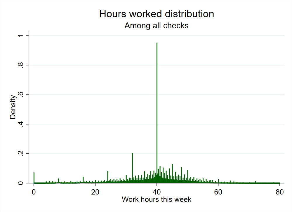
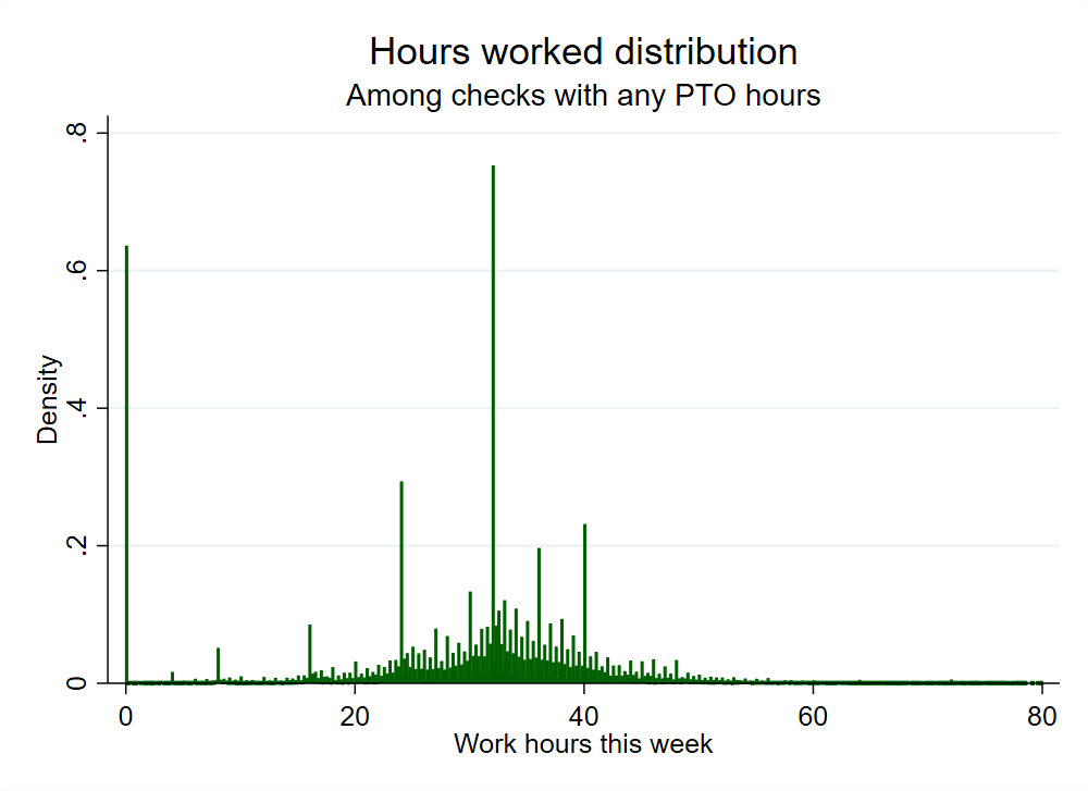
Figure 8: The right panel shows a histogram of hours worked when paid time off hours are positive ($\eta_{it}>0$). The left panel shows the unconditional distribution. While $\mathcal{B}\approx 11.6\%$, $P(h_{it}=40|n_{it}>0)\approx 2.7\%$.

Together, the two assumptions above imply that $p=P(K_{it}^{*}=1\textrm{ and }h_{it}=40)$ is identified as $\mathcal{B}-P(h_{it}=40|\eta_{it}>0)$. Figure 8 shows the conditional distribution of hours paid for work when the paycheck contains a positive number of PTO hours ($n_{it}>0$). The figure reveals that when moving from the unconditional (left panel) to positive-PTO conditional (right panel) distribution, most of the point mass at 40 hours moves away, largely concentrating now at 32 hours (corresponding to the PTO covering eight hours). Of the total bunching of $\mathcal{B}\approx 11.6\%$ in the unconditional distribution, I estimate that only $P(h_{it}=40|n_{it}>0)\approx 2.7\%$ are active bunchers, leaving $p\approx 8.9\%$. Thus roughly three quarters of the individuals at 40 hours are counterfactual rather than active bunchers.

As a secondary strategy, I estimate an upper bound for $p$ by using the assumption that the potential outcomes of counterfactual bunchers are relatively “sticky” over time. If the hours of counterfactual bunchers are at 40 for behavioral or administrative reasons, it is reasonable to assume that these external considerations are fairly static, preventing latent hours $h_{0it}$ from changing much between adjacent weeks. In particular, assume that in a given week $t$ nearly all of the counterfactual bunchers are also “non-changers” of hours from week $t-1$. Then:

$$p=P(h_{0it}=40)\approx P(h_{0it}=h_{0it-1}=40)\leq P(h_{it}=h_{i,t-1}=40),$$

where the inequality follows from $(h_{0it}=40)\implies(h_{it}=40)$ by Lemma 1. The probability $P(h_{it}=h_{i,t-1}=40)$ can be directly estimated from the data, yielding $p\leq 6\%$.

5.2 Estimation and inference

Given Theorem 1 and a value of $p$, computing bounds on the buncher ATE requires estimates of the right and left limits of the CDF and density of hours at the kink. I use the local polynomial density estimator of [16] (CJM), which is well-suited to estimating a CDF and its derivatives at boundary points. A local-linear CJM estimator of the left limit of the CDF and density at $k$, for instance, is:

$$(\hat{F}_{-}(k),\hat{f}_{-}(k))=\underset{(b_{1},b_{2})}{\operatorname{argmin}}\sum_{it:h_{it}<k}\left(F_{n}(h_{it})-b_{1}-b_{2}h_{it}\right)^{2}\cdot K\left(\frac{h_{it}-k}{\alpha}\right)$$ (10)

where $F_{n}(y)=\frac{1}{n}\sum_{it}\mathbbm{1}(h_{it}\leq y)$ is the empirical CDF of a sample of size $n$, $K(\cdot)$ is a kernel function, and $\alpha$ is a bandwidth. The right limits $F_{+}(k)$ and $f_{+}(k)$ are estimated analogously using observations for which $h_{it}>k$. I use a triangular kernel, and choose $h$ as follows: first, I use CJM’s mean-squared error minimizing bandwidth selector to produce bandwidth choices for the left and right limits at $k=40$. I then average the two bandwidths, and use this common bandwidth in the final calculation of both limits. In the full sample, the bandwidth chosen by this procedure is about 1.7 hours, and is somewhat larger for estimates that condition on a single industry.

To construct confidence intervals for parameters that are partially identified (e.g. the buncher ATE), I use adaptive critical values proposed by [31] and [49] that are valid for the underlying parameter. To easily incorporate sampling uncertainty in all of $\hat{F}_{-}(k),\hat{f}_{-}(k),\hat{F}_{+}(k),\hat{f}_{+}(k)$ and $\hat{p}$, I estimate variances by a cluster nonparametric bootstrap that resamples at the firm level. This allows arbitrary autocorrelation in hours across pay periods for a single worker, and between workers within a firm. All standard errors use 500 bootstrap samples.

5.3 Results of the bunching estimator: the buncher ATE

Table 3 reports treatment effect estimates based on Theorem 1, when $p$ is either assumed to be zero or is estimated by one of the two methods described in Section 5.1. The first row reports the corresponding estimate of the net bunching probability $\mathcal{B}-p$, while the second row reports the bounds on the buncher ATE $\mathbbm{E}[h_{0it}-h_{1it}|h_{it}=k,K_{it}^{*}=0]$. Within a fixed estimate of $p$, the bounds on the buncher ATE based on bi-log-concavity are quite informative: the upper and lower bounds are close to each other and precisely estimated. One can show from the expressions for the bounds in Theorem 1 that if $f_{0}(k)\approx f_{1}(k)$ and $p\approx 0$, the bounds will tend to be narrower when $F_{0}(k)$ is closer to $(1-\mathcal{B})/2$, i.e. the kink is close to the median of the latent hours distribution. This provides some intuition for why the bounds are reasonably narrow, since hours are roughly evenly divided to either side of 40 hours (cf. Figure 2).

	p=0	p from non-changers	p from PTO
Net bunching:	0.116	0.057	0.027
	[0.112, 0.120]	[0.055, 0.058]	[0.024, 0.030]
Buncher ATE	[2.614, 3.054]	[1.324, 1.435]	[0.640, 0.666]
	[2.493, 3.205]	[1.264, 1.501]	[0.574, 0.736]
———————–
Num observations	630217	630217	630217
Num clusters	566	566	566

Table 3: Estimates of net bunching $\mathcal{B}-p$ and the buncher ATE: $\Delta_{k}^{*}=\mathbbm{E}[h_{0it}-h_{1it}|h_{it}=k,K_{it}^{*}=0]$, across various strategies to estimate counterfactual bunching $p=P(K_{it}^{*}=1)$. Unit of analysis is a paycheck, and 95% bootstrap confidence intervals (in gray) are clustered by firm.

The PTO-based estimate of $p$ provides the most conservative treatment effect estimate, attributing roughly one quarter of the observed bunching to active rather than counterfactual bunchers. Nevertheless, this estimate still yields a highly statistically significant buncher ATE of about 2/3 of an hour, or 40 minutes. This estimate has the following interpretation: consider the group of workers that are in fact working 40 hours in a given pay period and are not counterfactual bunchers. Firms would ask this group to work on average about 40 minutes more that week if they were paid their straight-time wage for all hours, compared with a counterfactual in which they are paid their overtime rate for all hours. If we instead attribute all of the observed bunching mass to active bunchers ($p=0$), then the buncher ATE is estimated to be at least 2.6 hours. In Appendix E I also report estimates based on alternative shape constraints and assumptions about effect heterogeneity (with similar results).

5.4 Estimates of policy effects

I now use estimates of the buncher ATE and the results of Section 4.4 to estimate the overall causal effect of the FLSA overtime rule, and simulate changes based on modifying standard hours or the premium pay factor. Table 4 first reports an estimate of the buncher ATE expressed as a reduced-form hours demand elasticity, which I use as an input in these calculations. The next two rows report bounds on $\mathbbm{E}[h_{it}-h^{*}_{it}]$ and $\mathbbm{E}[h_{it}-h^{*}_{it}|h_{1it}\geq 40,K_{it}^{*}=0]$, respectively. The second row is the overall ex-post effect of the FLSA on hours, averaged over workers and pay periods, and the third row conditions on paychecks reporting at least 40 hours (omitting counterfactual bunchers). The final row reports an estimate of the effect of moving to double-time pay.

	p=0	p from non-changers	p from PTO
Buncher ATE as elasticity	[-0.188,-0.161]	[-0.088,-0.082]	[-0.041,-0.039]
	[-0.198,-0.154]	[-0.093,-0.078]	[-0.045,-0.035]
———————–
Average effect of FLSA on hours	[-1.466, -1.026]	[-0.727, -0.486]	[-0.347, -0.227]
	[-1.535, -0.977]	[-0.762, -0.463]	[-0.384, -0.203]
———————–
Avg. effect among directly affected	[-2.620, -1.833]	[-1.453, -0.972]	[-0.738, -0.483]
	[-2.733, -1.750]	[-1.518, -0.929]	[-0.812, -0.434]
———————–
Double-time, average effect on hours	[-2.604, -0.569]	[-1.239, -0.314]	[-0.580, -0.159]
	[-2.707, -0.547]	[-1.285, -0.300]	[-0.638, -0.143]

Table 4: Estimates of the buncher ATE expressed as an elasticity, the average ex-post effect of the FLSA $\mathbbm{E}[h_{it}-h_{it}^{*}]$,33 the effect among directly affected units $\mathbbm{E}[h_{it}-h_{it}^{*}|h_{it}\geq k,K^{*}_{it}=0]$ and predicted effects of a change to double-time. 95% bootstrap confidence intervals in gray, clustered by firm.

Taking the PTO-based estimate of $p$ as yielding a lower bound on treatment effects, the estimates suggest that workers work at least about 1/4 of an hour less on average in a given week than they would absent overtime regulation: about one third the magnitude of the buncher ATE. When I focus on those workers that are directly affected in a given week, the figure is about twice as high: roughly 30 minutes. Since my data has been restricted to hourly workers paid on a weekly basis, these estimates should be interpreted as holding for that population only. While one might assume that similar effects hold for hourly workers paid at other intervals (e.g. bi-weekly), speaking to the hours effects of the FLSA on salary workers is beyond the scope of this study.

Table 4 also suggests that a move to double-time pay would introduce a further reduction in hours comparable to the existing ex-post effect of the FLSA, but the bounds are wider. These estimates include the effects of possible adjustments to straight-time wages, which tend to attenuate the impact of the policy change. Appendix Table LABEL:otresults_nowage replicates Table 4 neglecting wage adjustments, which might be viewed as a short-run response to the FLSA before wages adjust.

Figure 9 breaks down estimates of the ex-post effect of the overtime rule by major industries, revealing considerable heterogeneity between them. The estimates suggest that Real Estate & Rental and Leasing as well as Wholesale Trade see the highest average reduction in hours. The least-affected industries are Health Care and Social Assistance and Professional Scientific and Technical, with the average worker working just about 6 minutes less per week due to the overtime rule. Appendix E reports estimates broken down by gender, finding that the FLSA has considerably higher effects on the hours of men compared with women.

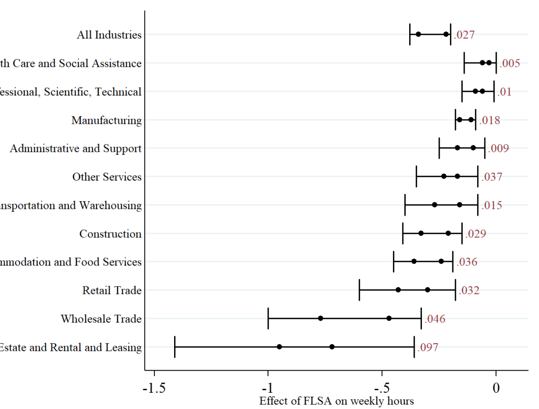
Figure 9: 95% confidence intervals for the effect of the FLSA on hours by industry, using PTO-based estimates of $p$ for each. Dots are point estimates of the upper and lower bounds. The number to the right of each range is the point estimate of the net bunching $\mathcal{B}-p$ for that industry.

Appendix Figure E.11 looks at the effect of changing the threshold for overtime hours $k$ from $40$ to alternative values $k^{\prime}$. The left panel reports estimates of the identified bounds on $\mathcal{B}^{[k^{\prime},\rho_{1}]}$ as well as point-wise 95% confidence intervals (gray) across values of $k^{\prime}$ between 35 and 45, for each of the three approaches to estimating $p$. In all cases, the upper bound on bunching approaches zero as $k^{\prime}$ is moved farther from $40$. This is sensible if the $h_{0}$ and $h_{1}$ distributions are roughly unimodal with modes around $40$: straddling of potential outcomes becomes less and less likely as one moves away from where most of the mass is. Appendix Figure E.10 shows these bounds as $k^{\prime}$ ranges all the way from $0$ to $80$, for the $p=0$ case.

When $p$ is estimated using PTO or non-changers between periods, we see that the upper bound of the identified set for $\mathcal{B}^{[k^{\prime},\rho_{1}]}$ in fact reaches zero quite quickly in $k^{\prime}$. Moving standard hours to $35$ is thus predicted to completely eliminate bunching due to the overtime kink in the short run, before any adjustment to latent hours (e.g. through changes to straight-time wages). The right panel of Appendix Figure E.11 shows estimates for the average effect on hours of changing standard hours, inclusive of wage effects (see Appendix LABEL:policyexpressions for details). Increases to standard hours cause an increase in hours per worker, as overtime policy becomes less stringent, and reductions to standard hours reduce hours. The size of these effects is not precisely estimated for changes larger than a couple of hours, however the range of statistically significant effects depends on $p$. Even for the preferred estimate of $p$ from PTO, increasing the overtime threshold as high as 43 hours is estimated to increase average working hours by an amount distinguishable from zero.

6 Implications of the estimates for overtime policy

The estimates from the preceding section suggest that FLSA regulation indeed has real effects on hours worked, in line with labor demand theory when wages do not fully adjust to absorb the added cost of overtime hours. When averaged over affected workers and across pay periods, I find that hourly workers in my sample work at least 30 minutes less per week than they would without the overtime rule. This lower bound is broadly comparable to the few causal estimates that exist in the literature, including [28] who assess the effects of expanding California’s daily overtime rule to cover men in 1980, and [12] who use the erosion of the salary threshold for exemption of white-collar jobs in real terms over the last several decades. By contrast, my estimates use an identification strategy that does not require focusing on the sub-population affected by a natural experiment, and are based on recent and administrative data.

My estimates speak to the substitutability of hours of labor between workers. The primary justifications for overtime regulation have been to reduce excessive workweeks, while encouraging hours to be distributed over more workers [22]. How well this plays out in practice hinges on how easily an hour of work can be moved from one worker to another or across time, from the perspective of the firm. The results of this paper find hours demand to be relatively inelastic: hours cannot be easily so reallocated between workers or weeks. This suggests that ongoing efforts to expand coverage of the FLSA overtime rule may have limited scope to dramatically affect the hours of U.S. workers.

Nevertheless, the overall impact of the FLSA overtime rule on workers is still notable. The data suggest that at least about $3\%$ and as many as about $12\%$ of workers’ hours are adjusted to the threshold introduced by the policy, indicating that it may have distortionary impacts for a significant portion of the labor force. The policy may also have important effects on unemployment. While a full assessment of the employment effects of the FLSA overtime rule is beyond the scope of this paper, my estimates of the hours effect can be used to build a back-of-the-envelope calculation. Following [27], I assume a value for the rate at which firms substitute labor for capital to obtain a “best-guess” estimate that the FLSA overtime rule creates about 700,000 jobs (see Appendix E.4 for details). To get an overall upper bound on the size of employment effects, one can instead attribute all of the bunching at 40 to the FLSA and assume that the total number of worker-hours is not reduced by the FLSA. By this estimate the FLSA increases employment by at most 3 million jobs, or roughly 3% among covered workers. A reasonable range of parameter values in this simple calculation rules out that the FLSA overtime rule has negative overall employment effects on hourly workers.

7 Conclusion

This paper has provided a new interpretation of the popular bunching-design method in the language of treatment effects, showing that the basic identifying power of the method is robust to a wide variety of underlying choice models. Across such models, the parameter of interest remains a reduced-form average treatment effect (local to the kink) between two appropriately-defined counterfactual choices, which is partially identified under a natural nonparametric assumption about those counterfactuals’ distributions. This provides conditions under which the bunching design can be useful to answer program evaluation questions in a variety of contexts, particularly beyond those in which the researcher is prepared to posit a parametric model of agents’ preferences.

By leveraging these insights with a new payroll dataset recording exact weekly hours paid at the individual level, I estimate that U.S. hourly workers subject to the Fair Labor Standard Act work shorter hours due to its overtime provision, which may lead to positive employment effects. Given the large amount of within-worker variation in hours observed, the modest size of the FLSA effects estimated in this paper suggest that firms do face significant incentives to maintain longer working hours, countervailing against the ones introduced by policies intended to reduce them.

Appendix A Main proofs

A.1 Proof of Theorem 1

In proving Theorem 1, we may relax somewhat the assumption that $h_{1}$ and $h_{0}$ are everywhere BLC (conditional on $K^{*}=0$). What we in fact need is for these distributions to each be “locally” BLC over a region containing the kink. This relaxation may be of interest when motivating the BLC assumption, as discussed in Appendix D.

Call a distribution function $F(h)$ locally BLC on an interval $N$, if $\ln F(h)$ and $\ln(1-F(h))$ are concave for $h\in N$. Given Assumption RANK, we know that there exist fixed values $\Delta^{*}_{0}$ and $\Delta^{*}_{1}$ such that $h_{0it}\in[k,k+\Delta_{it}]\textrm{ iff }h_{0it}\in[k,k+\Delta^{*}_{0}]$, and $h_{1it}\in[k-\Delta_{it},k]\textrm{ iff }h_{1it}\in[k-\Delta^{*}_{1},k]$. In the proof that follows we assume that conditional on $K^{*}_{it}=0$, $h_{0}$ is BLC on $[k,k+\Delta_{0}^{*}]$ and $h_{1}$ is BLC on $[k-\Delta^{*}_{1},k]$. This is of course implied if these distributions are globally BLC as assumed in the main text.

Let $\mathcal{B}^{*}:=P(h_{it}=k|K^{*}=0)$. Given Assumption RANK:

$$E[h_{0it}-h_{1it} |h_{it}=k,K_{it}^{*}=0]=\frac{1}{\mathcal{B}^{*}}\int_{F_{0|K^{*}=0}(k)}^{F_{0|K^{*}=0}(k)+\mathcal{B}^{*}}\{Q_{0|K^{*}=0}(u)-Q_{1|K^{*}=0}(u)\}du$$

$$=\frac{1}{\mathcal{B}^{*}}\int_{F_{0|K^{*}=0}(k)}^{F_{0|K^{*}=0}(k)+\mathcal{B}^{*}}\{Q_{0|K^{*}=0}(u)-k\}du+\frac{1}{\mathcal{B}^{*}}\int_{F_{1|K^{*}=0}(k)-\mathcal{B}^{*}}^{F_{1|K^{*}=0}(k)}\{k-Q_{1|K^{*}=0}(v)\}dv$$

$$=\frac{1}{\mathcal{B}^{*}}\int_{F_{0|K^{*}=0}(k)}^{F_{0|K^{*}=0}(k+\Delta_{0}^{*})}\{Q_{0|K^{*}=0}(u)-k\}du+\frac{1}{\mathcal{B}^{*}}\int_{F_{1|K^{*}=0}(k-\Delta^{*}_{1})}^{F_{1|K^{*}=0}(k)}\{k-Q_{1|K^{*}=0}(v)\}dv$$

To replace $F_{0|K^{*}=0}(k)+\mathcal{B}^{*}$ with $F_{0|K^{*}=0}(k+\Delta_{0}^{*})$ and $F_{1|K^{*}=0}(k)-\mathcal{B}^{*}$ with $F_{1|K^{*}=0}(k-\Delta^{*}_{1})$, we use Equation (2), which is established as Lemma 1 in Appendix B. A proof of Lemma 1 is provided below.

Consider first the implication of local BLC that $F_{d|K^{*}=0}(h)$ is log-concave on an interval between $k$ and $k+t$ for some $t$. In what follows, we will consider positive $t\in[0,\Delta_{0}^{*}]$ for $d=0$ and negative such $t\in[-\Delta_{1}^{*},0]$ for $d=1$). Concavity implies that a first-order Taylor expansion for $\log F_{d|K^{*}=0}(k+t)$ around $k$ overshoots: i.e. $\log F_{d|K^{*}=0}(k+t)\leq\log F_{d|K^{*}=0}(k)+t\cdot\frac{d}{dh}\log F_{d|K^{*}=0}(k)$. Similarly, that $\log(1-F_{d|K^{*}=0}(h))$ is concave on an interval $[k,k+t]$ implies that $\log(1-F_{d|K^{*}=0}(k+t))\leq\log(1-F_{d|K^{*}=0}(k))+t\cdot\frac{d}{dh}\log(1-F_{d|K^{*}=0}(k))$. These two inequalities can be rearranged to put upper and lower bounds on $F_{d|K^{*}=0}(k+t)$:

$$1-(1-F_{d|K^{*}=0}(k))e^{-\frac{f_{d|K^{*}=0}(k)}{1-F_{d|K^{*}=0}(k)}t}\leq F_{d|K^{*}=0}(k+t)\leq F_{d|K^{*}=0}(k)e^{\frac{f_{d|K^{*}=0}(k)}{F_{d|K^{*}=0}(k)}t}$$

An analagous expression is obtained in Theorem 1 of [21].

Defining $u=F_{0|K^{*}=0}(k+t)$, we can use the substitution $t=Q_{0|K^{*}=0}(u)-k$ to translate the above into bounds on the conditional quantile function of $h_{0it}$, evaluated at $u$:

$$\frac{F_{0|K^{*}=0}(k)}{f_{0|K^{*}=0}(k)}\cdot\ln\left(\frac{u}{F_{0|K^{*}=0}(k)}\right)\leq Q_{0|K^{*}=0}(u)-k\leq-\frac{1-F_{0|K^{*}=0}(k)}{f_{0|K^{*}=0}(k)}\cdot\ln\left(\frac{1-u}{1-F_{0|K^{*}=0}(k)}\right)$$

And similarly for $h_{1}$, letting $v=F_{1|K^{*}=0}(k-t)$:

$$\frac{1-F_{1|K^{*}=0}(k)}{f_{1|K^{*}=0}(k)}\cdot\ln\left(\frac{1-v}{1-F_{1|K^{*}=0}(k)}\right)\leq k-Q_{1|K^{*}=0}(v)\leq-\frac{F_{1|K^{*}=0}(k)}{f_{1|K^{*}=0}(k)}\cdot\ln\left(\frac{v}{F_{1|K^{*}=0}(k)}\right)$$

A lower bound for $E[h_{0it}-h_{1it}|h_{it}=k,K_{it}^{*}=0]$ is thus:

$$\frac{F_{0|K^{*}=0}(k)}{f_{0|K^{*}=0}(k)\cdot\mathcal{B}^{*}}\int_{F_{0|K^{*}=0}(k)}^{F_{0|K^{*}=0}(k)+\mathcal{B}^{*}}\ln\left(\frac{u}{F_{0|K^{*}=0}(k)}\right)du+\frac{1-F_{1|K^{*}=0}(k)}{f_{1|K^{*}=0}(k)\cdot\mathcal{B}^{*}}\int_{F_{1|K^{*}=0}(k)-\mathcal{B}^{*}}^{F_{1|K^{*}=0}(k)}\ln\left(\frac{1-v}{1-F_{1|K^{*}=0}(k)}\right)dv$$

$$=g(F_{0|K^{*}=0}(k),f_{0|K^{*}=0}(k),\mathcal{B}^{*})+h(F_{1|K^{*}=0}(k),f_{1|K^{*}=0}(k),\mathcal{B}^{*})$$

where

$$g(a,b,x) :=\frac{a}{bx}\int_{a}^{a+x}\ln\left(\frac{u}{a}\right)du=\frac{a^{2}}{bx}\int_{1}^{1+\frac{x}{a}}\ln\left(u\right)du$$

$$=\frac{a^{2}}{bx}\left.\left\{u\ln(u)-u\right\}\right|_{1}^{1+\frac{x}{a}}=\frac{a^{2}}{bx}\left\{\left(1+\frac{x}{a}\right)\ln\left(1+\frac{x}{a}\right)-\frac{x}{a}\right\}$$

$$=\frac{a}{bx}\left(a+x\right)\ln\left(1+\frac{x}{a}\right)-\frac{a}{b}$$

and

$$h(a,b,x):=\frac{1-a}{bx}\int_{a-x}^{a}\ln\left(\frac{1-v}{1-a}\right)dv=\frac{(1-a)^{2}}{bx}\int_{1}^{1+\frac{x}{1-a}}\ln\left(u\right)du=g(1-a,b,x)$$

Similarly, an upper bound is:

$$-\frac{1-F_{0|K^{*}=0}(k)}{f_{0|K^{*}=0}(k)(\mathcal{B}^{*})}\int_{F_{0|K^{*}=0}(k)}^{F_{0|K^{*}=0}(k)+\mathcal{B}^{*}}\ln\left(\frac{1-u}{1-F_{0|K^{*}=0}(k)}\right)du$$

$$\hskip 144.54pt-\frac{F_{1|K^{*}=0}(k)}{f_{1|K^{*}=0}(k)(\mathcal{B}^{*})}\int_{F_{1|K^{*}=0}(k)-\mathcal{B}^{*}}^{F_{1|K^{*}=0}(k)}\ln\left(\frac{v}{F_{1|K^{*}=0}(k)}\right)dv$$

$$=\tilde{g}(F_{0|K^{*}=0}(k),f_{0|K^{*}=0}(k),\mathcal{B}^{*})+\tilde{h}(F_{1|K^{*}=0}(k),f_{1|K^{*}=0}(k),\mathcal{B}^{*})$$

where

$$\tilde{g}(a,b,x) :=-\frac{1-a}{bx}\int_{a}^{a+x}\ln\left(\frac{1-u}{1-a}\right)du=-\frac{(1-a)^{2}}{bx}\int_{1-\frac{x}{1-a}}^{1}\ln\left(u\right)du$$

$$=\frac{(1-a)^{2}}{bx}\left.\left\{u-u\ln(u)\right\}\right|_{1-\frac{x}{1-a}}^{1}=\frac{1-a}{b}+\frac{1-a}{bx}\left(1-a-x\right)\ln\left(1-\frac{x}{1-a}\right)$$

$$=-g(1-a,b,-x)$$

and

$$\tilde{h}(a,b,x):=-\frac{a}{bx}\int_{a-x}^{a}\ln\left(\frac{v}{a}\right)dv=-\frac{a^{2}}{bx}\int_{1-\frac{x}{a}}^{1}\ln\left(u\right)du=\tilde{g}(1-a,b,x)=-g(a,b,-x)$$

Given $p$, we relate the $K^{*}=0$ conditional quantities to their unconditional analogues:

$$F_{0|K^{*}=0}(k)=\frac{F_{0}(k)-p}{1-p}\quad\textrm{ and }\quad F_{1|K^{*}=0}(k)=\frac{F_{1}(k)-p}{1-p}\quad\textrm{ and }\quad\mathcal{B}^{*}=\frac{\mathcal{B}-p}{1-p}$$

$$f_{0|K^{*}=0}(k)=\frac{f_{0}(k)}{1-p}\quad\textrm{ and }\quad f_{1|K^{*}=0}(k)=\frac{f_{1}(k)}{1-p}$$

Let $F(h)=P(h_{it}\leq h)$ be the CDF of the data, and define $f(h)=\frac{d}{dh}P(h_{it}\leq h)$ for $h\neq k$. By Proposition 2 and the BLC assumption, the above quantities are related to observables as:

$$F_{0}(k)=\lim_{h\uparrow k}F(h)+p,\quad\quad F_{1}(k)=F(k),\quad\quad f_{0}(k)=\lim_{h\uparrow k}f(h),\quad\textrm{ and }\quad f_{1}(k)=\lim_{h\downarrow k}f(h)$$

As shown by [21], BLC implies the existence of a continuous density function, which assures that the required density limits exist, and delivers Item 1. of the theorem.

To obtain the final result, note that the function $g(a,b,x)$ is homogeneous of degree zero. Thus $\Delta_{k}^{*}\in[\Delta^{L}_{k},\Delta^{U}_{k}],$ with

$$\Delta^{L}_{k}:=g\left(F_{-}(k),f_{-}(k),\mathcal{B}-p\right)+g\left(1-F(k),f_{+}(k),\mathcal{B}-p\right)$$

$$\Delta^{U}_{k}:=-g\left(1-p-F_{-}(k),f_{-}(k),p-\mathcal{B}\right)-g\left(F(k)-p,f_{+}(k),p-\mathcal{B}\right)$$

where $-$ and $+$ subscripts denote left and right limits. The bounds are sharp as CHOICE, CONVEX and RANK imply no further restrictions on the potential outcome distributions.

A.2 Proof of Lemma 1

Theorem 1 makes use of Equation (2), which relates observable choices $h_{it}$ to the counterfactual choices $h_{0it}$ and $h_{1it}$. The result is stated formally in Appendix B as Lemma 1, but I include the proof here as it is central to the identification logic. This proof follows the notation of Appendix B, dropping the $t$ index from observational units for simplicity. I also use the generalized bunching design setting described in Appendix B, where the continuous function $h_{i}(\mathbf{x})$ relating hours to choice variables can vary by $i$.

The proof proceeds in the following two steps:

1. First, I show that $h_{0i}\leq k$ implies that $h_{i}=h_{0i}$, and similarly $h_{1i}\geq k$ implies that $h_{i}=h_{1i}$. This holds under CONVEX but also under the weaker assumption of WARP.

2. Second, I show that under CONVEX $h_{i}<k\implies h_{i}=h_{0i}$ and $h_{i}>k\implies h_{i}=h_{1i}$.

Item i) above establishes the first and third cases of Lemma 1. The only remaining possible case is that $h_{1i}\leq k\leq h_{0i}$. However, to finish establishing Lemma 1, we also need the reverse implication: that $h_{1i}\leq k\leq h_{0i}$ implies $h_{i}=k$. This comes from taking the contrapositive of each of the two claims in item ii).

Proof of i): Let $\mathcal{X}_{0i}=\{\mathbf{x}:h_{i}(\mathbf{x})\leq k\}$ and $\mathcal{X}_{1i}=\{\mathbf{x}:h_{i}(\mathbf{x})\geq k\}$. If $h_{0i}\leq k$, then by CHOICE $\mathbf{x}_{B_{0i}}$ is in $\mathcal{X}_{0}$, where for any budget constraint $B$, $(z_{Bi},\mathbf{x}_{Bi})$ are the choices the decision-maker would make under $B$. Since $B_{i}(\mathbf{x})=B_{0i}(\mathbf{x})$ for all $\mathbf{x}\in\mathcal{X}_{0}$, it follows that $z_{B_{0i}i}\geq B_{i}(\mathbf{x}_{B_{0i}i})$, i.e. the decision-maker’s choice under $B_{0}$ is feasible under the kinked budget constraint $B$. Note that $B_{i}(\mathbf{x})\geq B_{0i}(\mathbf{x})$ for all $\mathbf{x}$. By WARP then $(z_{B_{i}i},\mathbf{x}_{B_{i}i})=(z_{B_{0i}i},\mathbf{x}_{B_{0i}i})$. Thus $h_{i}=h_{i}(\mathbf{x}_{B_{i}i})=h_{i}(\mathbf{x}_{B_{0i}i})=h_{0i}$. So $h_{0i}\leq k\implies h_{i}=h_{0i}$. By the same logic we can show that $h_{1i}\geq k\implies h_{i}=h_{1i}$.

Proof of ii): For any convex budget function $B(\mathbf{x})$, $(z_{Bi},\mathbf{x}_{Bi})=\textrm{argmax}_{z,\mathbf{x}}\left\{u_{i}(z,\mathbf{x})\textrm{ s.t. }z\geq B(\mathbf{x})\right\}$. If $u_{i}(z,\mathbf{x})$ is strictly quasi-concave, then the RHS exists and is unique since it maximizes $u_{i}$ over the convex domain $\{(z,\mathbf{x}):z\geq B(\mathbf{x})\}$. Furthermore, by monotonicity of $u(z,\mathbf{x})$ in $z$ we may substitute in the constraint $z=B(\mathbf{x})$ and write

$$\mathbf{x}_{Bi}=\textrm{argmax}_{\mathbf{x}}u_{i}(B(\mathbf{x}),\mathbf{x})$$

Suppose that $h_{i}(\mathbf{x}_{Bi})\neq k$, and consider any $\mathbf{x}\neq\mathbf{x}_{Bi}$ such that $h_{i}(\mathbf{x})\neq k$. Let $\tilde{\mathbf{x}}=\theta\mathbf{x}+(1-\theta)\mathbf{x}^{*}$ where $\mathbf{x}^{*}=\mathbf{x}_{Bi}$ and $\theta\in(0,1)$. Since $B(\mathbf{x})$ is convex in $\mathbf{x}$ and $u_{i}(z,\mathbf{x})$ is weakly decreasing in $z$:

$$u_{i}(B(\tilde{\mathbf{x}}),\tilde{\mathbf{x}})\geq u_{i}(\theta B(\mathbf{x})+(1-\theta)B(\mathbf{x}^{*}),\tilde{\mathbf{x}})>\min\{u_{i}(B(\mathbf{x}),\mathbf{x}),u_{i}(B(\mathbf{x}^{*}),\mathbf{x}^{*})\}=u_{i}(B(\mathbf{x}),\mathbf{x})$$ (A.1)

where I have used CONVEX in the second step, and that $\mathbf{x}^{*}$ is a maximizer in the third. This result implies that for any such $\mathbf{x}\neq\mathbf{x}^{*}$, if one draws a line between $\mathbf{x}$ and $\mathbf{x}^{*}$, the function $u_{i}(B(\mathbf{x}),\mathbf{x})$ is strictly increasing as one moves towards $\mathbf{x}^{*}$. When $\mathbf{x}$ is a scalar, this argument is used by [8] (see Lemma A1 therein) to show that $u_{i}(B(\mathbf{x}),\mathbf{x})$ is strictly increasing to the left of $\mathbf{x}^{*}$, and strictly decreasing to the right of $\mathbf{x}^{*}$. Note that for any (binding) linear budget constraint $B(\mathbf{x})$, the result still holds without monotonicity of $u_{i}(z,\mathbf{x})$ in $z$. This is useful for Theorem 1* of Appendix C in which some workers choose their hours.

For any function $B$, let $u_{Bi}(\mathbf{x})=u_{i}(B(\mathbf{x}),\mathbf{x})$, and note that

$$u_{B_{i}i}(\mathbf{x})=\begin{cases}u_{B_{0i}i}(\mathbf{x})&\hskip 5.69046pt\textrm{if }\hskip 5.69046pt\mathbf{x}\in\mathcal{X}_{0i}\\ u_{B_{1i}i}(\mathbf{x})&\hskip 5.69046pt\textrm{if }\hskip 5.69046pt\mathbf{x}\in\mathcal{X}_{1i}\end{cases}$$

where $B_{i}$ is the actual, kinked budget constraint faced by $i$. Let $\mathbf{x}_{ki}$ be the unique maximizer of $u_{B_{i}i}(\mathbf{x})$, where $h_{i}=h_{i}(\mathbf{x}_{ki})$. Suppose that $h_{i}<k$. Suppose furthermore that $h_{0i}\neq h_{i}$, with $h_{0i}=h_{i}(\mathbf{x}_{0i})$ and $\mathbf{x}_{0i}$ the maximizer of $u_{B_{0i}i}(\mathbf{x})$. Note that we must have that $\mathbf{x}_{0i}\notin\mathcal{X}_{0i}$, because $B_{0i}=B_{i}$ in $\mathcal{X}_{0i}$ so we can’t have $u_{B_{0i}i}(\mathbf{x}_{0i})>u_{B_{0i}i}(\mathbf{x}_{ki})$ (since $\mathbf{x}_{ki}$ maximizes $u_{B_{i}}(\mathbf{x})$). Thus $h_{0i}>k$.

By continuity of $h_{i}(\mathbf{x})$, $\mathcal{X}_{0i}$ is a closed set and $\mathbf{x}_{ki}$ belongs to the interior of $\mathcal{X}_{0i}$. Thus, while $\mathbf{x}_{0i}$ is not in $\mathcal{X}_{0i}$, there exists a point $\tilde{\mathbf{x}}\in\mathcal{X}_{0i}$ along the line between $\mathbf{x}_{0i}$ to $\mathbf{x}_{ki}$. Since $h_{i}\neq k$ and $h_{0i}\neq k$, Eq. (A.1) then implies that $u_{B_{i}i}(\tilde{\mathbf{x}})>u_{B_{i}i}(\mathbf{x}_{0i})$. Since $u_{B_{0i}i}(\mathbf{x})=u_{B_{i}i}(\mathbf{x})$ for all $\mathbf{x}$ in $\mathcal{X}_{0i}$, it follows that $u_{B_{0i}i}(\tilde{\mathbf{x}})>u_{B_{0i}i}(\mathbf{x}_{0i})$. However, this contradicts the premise that $\mathbf{x}_{0i}$ maximizes $u_{B_{0i}i}(\mathbf{x})$. Thus, $h_{i}<k$ implies $h_{i}=h_{0i}$. Figure A.1 depicts the logic visually. The proof that $h_{i}>k$ implies $h_{i}=h_{1i}$ is analogous.

Figure A.1: Depiction of the step establishing $(h<k)\implies(h=h_{0})$ in the proof of Lemma 1. Since the result considers a single decision-maker $i$, I supress this index in the Figure. In this example $z=(x_{1},x_{2})$ and $y(\mathbf{x})=x_{1}+x_{2}$. Proof is by contradiction. If $h_{0}\neq Y$, then $\mathbf{x}^{*}_{k}\neq\mathbf{x}^{*}_{0}$, where $\mathbf{x}^{*}_{k}$ and $\mathbf{x}^{*}_{0}$ are the unique maximizers of $u_{B}(\mathbf{x})$ and $u_{B_{0}}(\mathbf{x})$, respectively. By Equation A.1, we have that the function $u_{B_{0}}(\mathbf{x})$, depicted heuristically as a solid black curve, is strictly increasing as one moves along the dotted line from $\mathbf{x}_{k}^{*}$ towards $\mathbf{x}^{*}_{0}$. Similarly, the function $u_{B_{0}}(\mathbf{x})$, depicted as a solid blue curve, is strictly increasing as one moves in the opposite direction along the same line, from $\mathbf{x}_{0}^{*}$ towards $\mathbf{x}^{*}_{k}$. By the assumption that $h<k$, then using continuity of $h(\mathbf{x})$ it must be the case that $\mathbf{x}^{*}_{k}$ lies in the interior of $\mathcal{X}_{0}$, the set of $\mathbf{x}$’s that make $h(\mathbf{x})\leq k$. This means that there is some interval of the dotted line that is within $\mathcal{X}_{0}$. On this interval, the functions $B_{0}$ and $B$ are equal, and thus so must be the functions $u_{B}$ and $u_{B_{0}}$. Since the same function cannot be both strictly increasing and strictly decreasing, we have obtained a contradiction.

A.3 Proof of Theorem 2

This proof continues with the notation of Appendix B, using $i$ rather than $it$ indices. Throughout this proof we let $h_{i}(\rho,k)=h_{i}(\rho)$, given Assumption SEPARABLE. By Lemmas 2 and 3 established in Appendix B, the effect of changing $k$ on bunching is:

$$\partial_{k}\left\{\mathcal{B}-p(k)\right\} =-\frac{\partial}{\partial k}\int_{\rho_{0}}^{\rho_{1}}f_{\rho}(k)\mathbbm{E}\left[\left.\frac{h_{i}(\rho)}{d\rho}\right|h_{i}(\rho)=k\right]d\rho$$

$$=-\int_{\rho_{0}}^{\rho_{1}}\frac{\partial}{\partial k}\left\{f_{\rho}(k)\mathbbm{E}\left[\left.\frac{h_{i}(\rho)}{d\rho}\right|h_{i}(\rho)=k\right]\right\}d\rho=\int_{\rho_{0}}^{\rho_{1}}\partial_{\rho}f_{\rho}(k)d\rho=f_{1}(k)-f_{0}(k)$$

Turning now to the total effect on average hours.

$$\partial_{k}E[h_{i}^{[k,\rho_{1}]}] =\partial_{k}\left\{P(h_{i}(\rho_{0})<k)\mathbbm{E}[h_{i}(\rho_{0})|h_{i}(\rho_{0})<k]\right\}+k\partial_{k}\left(\mathcal{B}^{[k,\rho_{1}]}-p(k)\right)+\mathcal{B}^{[k,\rho_{1}]}-p(k)$$

$$\hskip 144.54pt+\partial_{k}\left\{P(h_{i}(\rho_{1})>k)\mathbbm{E}[h_{i}(\rho_{1})|h_{i}(\rho_{1})>k]\right\}$$

$$=\partial_{k}\int_{-\infty}^{k}y\cdot f_{\rho_{0}}(y)\cdot dy+k\left(f_{0}(k)-f_{1}(k)\right)+\mathcal{B}^{[k,\rho_{1}]}-p(k)+\partial_{k}\int_{k}^{\infty}y\cdot f_{\rho_{1}}(y)\cdot dy$$

$$=\cancel{kf_{0}(k)}+\cancel{k\left(f_{1}(k)-f_{0}(k)\right)}+\mathcal{B}^{[k,\rho_{1}]}-p(k)-\cancel{kf_{1}(k)}$$

Meanwhile: $\partial_{\rho_{1}}\mathbbm{E}[h_{i}^{[k,\rho_{1}]}]=-\int_{k}^{\infty}f_{\rho_{1}}(y)\mathbbm{E}\left[\left.\frac{dh_{i}(\rho_{1})}{d\rho}\right|h_{i}(\rho_{1})=y\right]dy$ follows directly from Lemma 2 and differentiating both sides with respect to $\rho_{1}$, and thus

$$\partial_{\rho_{1}}E[h_{i}^{[k,\rho_{1}]}]=k\partial_{\rho_{1}}\mathcal{B}^{[k,\rho_{1}]}+\partial_{\rho_{1}}\left\{P(h_{i}(\rho_{1})>k)\mathbbm{E}[h_{i}(\rho_{1})|h_{i}(\rho_{1})>k]\right\}=k\partial_{\rho_{1}}\mathcal{B}^{[k,\rho_{1}]}+\int_{k}^{\infty}y\cdot\partial_{\rho_{1}}f_{\rho_{1}}(y)\cdot dy$$

$$=-kf_{\rho_{1}}(k)\mathbbm{E}\left[\left.\frac{h_{i}(\rho_{1})}{d\rho}\right|h_{i}(\rho_{1})=k\right]-\int_{k}^{\infty}y\cdot\partial_{y}\left\{f_{\rho_{1}}(y)\mathbbm{E}\left[\left.\frac{dh_{i}(\rho_{1})}{d\rho}\right|h_{i}(\rho_{1})=y\right]\right\}dy$$

$$=\cancel{-kf_{\rho_{1}}(k)\mathbbm{E}\left[\left.\frac{h_{i}(\rho_{1})}{d\rho}\right|h_{i}(\rho_{1})=k\right]}+\cancel{\left.yf_{\rho_{1}}(y)\mathbbm{E}\left[\left.\frac{dh_{i}(\rho_{1})}{d\rho}\right|h_{i}(\rho_{1})=y\right]\right|_{\infty}^{k}}$$

$$\hskip 216.81pt-\int_{k}^{\infty}f_{\rho_{1}}(y)\mathbbm{E}\left[\left.\frac{dh_{i}(\rho_{1})}{d\rho}\right|h_{i}(\rho_{1})=y\right]dy$$

where I have used Lemma 2 with the Leibniz rule (establishing Item 3 in Theorem 2) as well as Lemma 3 in the third step, and then integration by parts along with the boundary condition that $\lim_{y\rightarrow\infty}y\cdot f_{\rho_{1}}(y)=0$, implied by Assumption SMOOTH.

Appendix B Identification in a generalized bunching design

This section presents some generalizations of the bunching-design model used in the main text. While the FLSA will provide a running example throughout, I largely abstract from the overtime context to emphasize the general applicability of the results.

To facilitate comparison with the existing literature on bunching at kinks – which has mostly considered cross-sectional data – I throughout this section suppress time indices and use the single index $i$ to refer to each unit of observation (a paycheck in the overtime setting). Further, the “running variable” of the bunching design is typically denoted by $Y$ rather than $h$, and so the random variable $Y_{i}$ will play the role of $h_{it}$ from the main text. This is done to emphasize the link to the treatment effects literature, while also allowing a distinction that is in some cases useful (e.g. in the overtime setting, models in which hours of pay for work differ from actual hours of work).

B.1 The policy environment

Here we abstract from the conventional piece-wise linear kink setting that appears in tax examples as well as the main body of this paper. Consider a population of observational units indexed by $i$. For each $i$, a decision-maker $d(i)$ chooses a point $(z,\mathbf{x})$ in some space $\mathcal{X}\subseteq\mathbbm{R}^{m+1}$ where $z$ is a scalar and $\mathbf{x}$ a vector of $m$ components, subject to a constraint of the form:

$$z\geq\textrm{max}\{B_{0i}(\mathbf{x}),B_{1i}(\mathbf{x})\}$$ (B.2)

The functions $B_{0i}(\mathbf{x})$ and $B_{1i}(\mathbf{x})$ are taken to be continuous and weakly convex functions of the vector $\mathbf{x}$, and assume that there exist continuous scalar functions $y_{i}(\mathbf{x})$ and a scalar $k$ such that:

$$B_{0i}(\mathbf{x})>B_{1i}(\mathbf{x})\textrm{ whenever }y_{i}(\mathbf{x})<k\quad\textrm{ and }\quad B_{0i}(\mathbf{x})<B_{1i}(\mathbf{x})\textrm{ whenever }y_{i}(\mathbf{x})>k$$

The value $k$ is taken to be common to all units $i$, and is assumed to be known by the researcher. In the overtime setting, $y_{i}(\mathbf{x})$ represents the hours of work for which a worker is paid in a given week, $k=40$, and $B_{0i}(\mathbf{x})=w_{i}y_{i}(\mathbf{x})$ and $B_{1i}(\mathbf{x})=1.5w_{i}y_{i}(\mathbf{x})-20w_{i}$. In most applications of the bunching design, the decision-maker $d(i)$ is simply $i$ themself, for example a worker choosing their labor supply subject to a tax kink. In the overtime application however $i$ is a worker-week pair, and $d(i)$ is the worker’s firm.

Let $X_{i}$ be $i$’s realized outcome of $\mathbf{x}$, and $Y_{i}=y_{i}(X_{i})$. I assume that $Y_{i}$ is observed by the econometrician, but not that $X_{i}$ is. In the overtime setting this means that the econometrician observes hours for which workers are paid, but not necessarily all choices made by firms that pin down those hours (for example, how many hours to allow the worker to stay “on the clock" during paid breaks–see Section B.3).

In general, the functions $B_{0i}$, $B_{1i}$ will represent a schedule of some kind of “cost” as a function of the choice vector $\mathbf{x}$, with two regimes of costs that are separated by the condition $y_{i}(\mathbf{x})=k$, characterizing the locus of points at which the two cost functions cross. Let $B_{i}(\mathbf{x}):=\textrm{max}\{B_{0i}(\mathbf{x}),B_{1i}(\mathbf{x})\}$ denote the actual constraint function that applies to $z$. A budget constraint like Eq. $z\geq B_{i}(\mathbf{x})$ is typically “kinked” because while the function $B_{i}(\mathbf{x})$ is continuous, it will generally be non-differentiable at the $\mathbf{x}$ for which $y_{i}(\mathbf{x})=k$. While the functions $B_{0}$, $B_{1}$ and $y$ can all depend on $i$, I will often suppress this dependency for clarity of notation.

Discussion of the general model:

In the most common cases from the literature, no distinction is made between the “running variable” $y$ of the kink and any underlying choice variables $\mathbf{x}$. This corresponds to a setting in which $\mathbf{x}$ is a scalar and $y_{i}(x)=x$. For example, the seminal bunching design papers [45] and [18] considered progressive taxation with $z$ being tax liability (or credits), $y=x$ corresponding to taxable income, and $B_{0}$ and $B_{1}$ linear tax functions on either side of a threshold $y$ between two adjacent tax/benefit brackets. Similarly, in the overtime context, the functions $B_{0}$ and $B_{1}$ are linear and only depend on hours $y_{i}(\mathbf{x})$, as depicted in Figure B.2. Appendix LABEL:sec:moreid discusses a tax setting in the literature in which the functions $B_{0}$ and $B_{1}$ are linear but depend directly on a vector $\mathbf{x}$ of two components. This represents a non-standard bunching-design setting, but fits naturally within the framework of this section.

Figure B.2: Definition of counterfactual cost functions $B_{0}$ and $B_{1}$ that firms could have faced, absent the overtime kink. Regardless of what choice variables are in $\mathbf{x}$, these functions only depend on $y_{i}(\mathbf{x})$ and are thus depicted as a function of $y$. Dashed lines show the rest of actual kinked-cost function in comparison to the counterfactual as a solid line. Note that we use the notation $y$ here to indicate hours, rather than the $h$ used in the main text.

Even when the functions $B_{0}$ and $B_{1}$ only depend on $\mathbf{x}$ through $y_{i}(\mathbf{x})$, as in standard settings, the bunching design is compatible with models in which multiple margins of choice respond to the incentives provided by the kink. As discussed in the overtime context, the econometrician may be agnostic as to even what the full set of components of $\mathbf{x}$ are, with $B_{0i}(\cdot)$, $B_{1i}(\cdot)$, and $y_{i}(\cdot)$ depending only on various subsets of the $\mathbf{x}$ that are possibly heterogeneous by $i$ (this is allowable because $y$ need only be continuous in $\mathbf{x}$, and the cost functions only need to be continuous and weakly convex in $\mathbf{x}$, both of which are compatible with zero dependence on some of its components). Appendix LABEL:sec:otherexamples gives an example in which the overtime kink gives firms an incentive to reduce bonuses, which appear in firm costs but not in the kink the variable $y$.

In general, the bunching design allows us to conduct causal inference on $Y_{i}=y_{i}(X_{i})$, but not directly on the underlying choice variables $X_{i}$. For example in the overtime setting with possible evasion (see Sec. B.3), bunching at 40 hours will be informative about the effect of a move from $B_{0}$ to $B_{1}$ on reported hours worked $y$. However, it will not disentangle whether the effect on hours actually worked is attenuated by, for example, an increase in hours worked off-the-clock. The empirical setting of [4] provides another environment in which this point is relevant (see Appendix LABEL:sec:otherexamples).

B.2 Potential outcomes as counterfactual choices

Here I restate slightly more general versions of assumptions CONVEX and CHOICE from Section 4, in the present notation. As in Section 4, let us define a pair of potential outcomes as what would occur if the decision-maker faced either of the functions $B_{0}$ or $B_{1}$ globally, without the kink.

Definition ((potential outcomes)).

Let $Y_{0i}$ be the value of $y_{i}(\mathbf{x})$ that would occur for unit $i$ if $d(i)$ faced the constraint $z\geq B_{0}(\mathbf{x})$, and let $Y_{1i}$ be the value that would occur under the constraint $z\geq B_{1}(\mathbf{x})$.

I again make explicit the assumption that these potential outcomes reflect choices made by the decision-maker. For any function $B$ let $Y_{Bi}$ be the outcome that would occur under the choice constraint $z\geq B(\mathbf{x})$, with $Y_{0i}$ and $Y_{1i}$ shorthands for $Y_{B_{0i}i}$ and $Y_{B_{0i}i}$, respectively. In this notation, the actual outcome $Y_{i}$ observed by the econometrician is equal to $Y_{B_{i}i}$.

Assumption (CHOICE (perfect manipulation of $y$)).

For any function $B(\mathbf{x})$, $Y_{Bi}=y_{i}(\mathbf{x}_{B_{i}})$, where $(z_{Bi},\mathbf{x}_{Bi})$ is the choice that $d(i)$ would make under the constraint $z\geq B(\mathbf{x})$.

Assumption CHOICE rules out for example optimization error, which could limit the decision-maker’s ability to exactly manipulate values of $\mathbf{x}$ and hence $y$. It also takes for granted that counterfactual choices are unique, and rules out some kinds of extensive margin effects in which a decision-maker would not choose any value of $Y$ at all under $B_{1}$ or $B_{0}$. Note that CHOICE here is slightly stronger than the version given in the main text in that it applies to all functions $B$, not just $B_{0}$, $B_{1}$ and $B_{k}$ (this is useful for Theorem 2).

The central behavioral assumption that allows us to reason about the counterfactuals $Y_{0}$ and $Y_{1}$ is that decision-makers have convex preferences over $(c,\mathbf{x})$ and dislike costs $z$:

Assumption (CONVEX (strictly convex preferences except at kink, decreasing in $z$)).

For each $i$ and any function $B(\mathbf{x})$, choice is $(z_{Bi},\mathbf{x}_{Bi})=\textrm{argmax}_{z,\mathbf{x}}\{u_{i}(z,\mathbf{x}):z\geq B(\mathbf{x})\}$ where $u_{i}(z,\mathbf{x})$ is weakly decreasing in $z$ and satisfies

$$u_{i}(\theta z+(1-\theta)z^{*},\theta\mathbf{x}+(1-\theta)\mathbf{x}^{*})>\min\{u_{i}(z,\mathbf{x}),u_{i}(z^{*},\mathbf{x}^{*})\}$$

for any $\theta\in(0,1)$ and points $(z,\mathbf{x})$,$(z^{*},\mathbf{x}^{*})$ such that $y_{i}(\mathbf{x})\neq k$ and $y_{i}(\mathbf{x}^{*})\neq k$.

Note: The function $u_{i}(\cdot)$ represents preferences over choice variables for unit $i$, but the preferences are those of the decision maker $d(i)$. I avoid more explicit notation like $u_{d(i),i}(\cdot)$ for brevity. In the overtime setting with firms choosing hours, $u_{i}(z,\mathbf{x})$ corresponds to the firm’s profit function $\pi$ as a function of the hours of a particular worker this week, and costs this week $z$ for that worker.

Note: The second part of Assumption CONVEX is implied by strict quasi-concavity of the function $(z,\mathbf{x})$, corresponding to strictly convex preferences. However it also allows for decision-makers preferences to have “two peaks”, provided that one of the peaks is located exactly at the kink. This is useful in cases in which the kink is located at a point that has particular value to decision-makers, such as firms setting weekly hours. For example, suppose that firms choose hours only $\mathbf{x}=h$, and have preferences of the form:

$$u_{i}(z,h)=af(h)+\phi\cdot\mathbbm{1}(h=40)-z$$ (B.3)

where $f(h)$ is strictly concave. This allows firms to have a behavioral “bias” towards 40 hours, or to extract extra profits when $h=40$ exactly. Figure B.3 depicts an example of such preferences, given an arbitrary linear budget function $B(h)$. Note that if a mass of firms were to have preferences of this form, then it would be natural to expect bunching in the distributions of $h_{0it}$ and $h_{1it}$, which I allow in Section 5.

Figure B.3: An example of preferences that satisfy CONVEX but are not strictly convex, cf. Eq. (B.3).

Note: Some departures from CONVEX are allowable without compromising it’s main implication for the bunching-design, which is given in Lemma 1 below. If $B_{0}$ and $B_{1}$ are linear in $\mathbf{x}$ and the constraint $z\geq B(\mathbf{x})$ can be assumed to bind (hold as an equality), then the assumption that $u_{i}$ is decreasing in $z$ from CONVEX can be dropped (see Assumption CONVEX* in Appendix C). If by contrast $B_{0}$ and $B_{1}$ were strictly (rather than weakly) convex, strict convexity of preferences could be replaced with weakly convex preferences along with an assumption that $u_{i}$ are strictly decreasing in $z$ (see Eq. (A.1) in the Proof of Lemma 1).

Note: The notation of Assumption CONVEX does not make explicit any dependence of the functions $u_{i}(\cdot)$ on the choices made for other observational units $i^{\prime}\neq i$. When the functions $u_{i}(\cdot)$ are indeed invariant over such counterfactual choices, we have a version of the no-interference condition of the stable unit treatment values assumption (SUTVA). Maintaining SUTVA is not necessary to define treatment effects in the bunching design, provided that the variables $y$ and $z$ can be coherently defined at the individual unit $i$ level (see Appendix LABEL:app:inter for details). Nevertheless, the interpretation of the treatment effects identified by the bunching design is most straightforward when SUTVA does hold. This assumption is standard in the bunching design.

A weaker assumption than CONVEX that still has identifying power is simply that decision-makers’ choices do not violate the weak axiom of revealed preference:

Assumption (WARP (rationalizable choices)).

Consider two budget functions $B$ and $B^{\prime}$ and any unit $i$. If $d(i)$’s choice under $B^{\prime}$ is feasible under $B$, i.e. $z_{B^{\prime}i}\geq B(\mathbf{x}_{B^{\prime}i})$, then $(z_{Bi},\mathbf{x}_{Bi})=(z_{B^{\prime}i},\mathbf{x}_{B^{\prime}i})$.

I make the stronger assumption CONVEX for most of the identification results, but Assumption WARP still allows a version of many of them in which equalities become weak inequalities, indicating a degree of robustness with respect to departures from convexity (see Propositions 1 and 2 below). Note that the monotonicity assumption in CONVEX implies that choices will always satisfy $z=B(\mathbf{x})$, i.e. agents’ choices will lay on their cost functions (despite Eq. B.2 being an inequality, indicating “free-disposal”).

B.3 Examples from the general choice model in the overtime setting

To demonstrate the flexibility of the general choice model CONVEX, I below present some examples for the overtime setting. These examples are meant only to be illustrative, and each could apply to a different subset of units in the population. In these examples we continue to take the decision-maker for a given unit to be the firm employing that worker.

Example 1: Substitution from bonus pay
Let the firm’s choice vector be $\mathbf{x}=(h,b)^{\prime}$, where $b\geq 0$ indicates a bonus (or other fringe benefit) paid to the worker. Firms may find it optimal to offer bonuses to improve worker satisfaction and reduce turnover. Suppose firm preferences are: $\pi(z,h,b)=f(h)+g(z+b-\nu(h))-z-b$, where $z$ continues to denote wage compensation this week, $z+b-\nu(h)$ is the worker’s utility with $\nu(h)$ a convex disutility from labor $h$, and $g(\cdot)$ increasing and concave. In this model firms will choose the surplus maximizing choice of hours $h_{m}:=\textrm{argmax}_{h}f(h)-\nu(h)$, provided that the corresponding optimal bonus is non-negative. Bonuses fully adjust to counteract overtime costs, and $h_{0}=h_{1}=h_{m}$.

Example 2: Off-the-clock hours and paid breaks
Suppose firms choose a pair $\mathbf{x}=(h,o)^{\prime}$ with $h$ hours worked and $o$ hours worked “off-the-clock”, such that $y(\mathbf{x})=h-o$ are the hours for which the worker is ultimately paid. Evasion is harder the larger $o$ is, which could be represented by firms facing a convex evasion cost $\phi(o)$, so that firm utility is $\pi(z,h,o)=f(h)-\phi(o)-z$. This model can also include some firms voluntarily offering paid breaks by allowing $o$ to be negative.

Example 3: Complementaries between workers or weeks
Suppose the firm simultaneously chooses the hours $\mathbf{x}=(h,g)$ of two workers according to production that is isoelastic in a CES aggregate ($g$ could also denote planned hours next week): $\pi(z,h,g)=a\cdot\left((\gamma h^{\rho}+g^{\rho})^{1/\rho}\right)^{1+\frac{1}{\epsilon}}-z$ with $\gamma$ a relative productivity shock. Let $g^{*}$ denote the firm’s optimal choice of hours for the second worker. Optimal $h$ then maximizes $\pi(z,h,g^{*})$ subject to $z=B(h)$, as if the firm faced a single-worker production function of $f(h)=a\cdot\left((\gamma h^{\rho}+{g^{*}}^{\rho})^{1/\rho}\right)^{1+\frac{1}{\epsilon}}$. This function is more elastic than $a\cdot h^{1+\frac{1}{\epsilon}}$ provided that $\rho<1+1/\epsilon$, attenuating the response to an increase in $w$ implied by a given $\epsilon$. Section 4.4 discusses how complementaries affect the final evaluation of the FLSA.

B.4 Observables in the kink bunching design

Lemma 1 outlines the core consequence of Assumption CONVEX for the relationship between observed $Y_{i}$ and the potential outcomes introduced in the last section:

Lemma 1 ((realized choices as truncated potential outcomes)).

Under Assumptions CONVEX and CHOICE, the outcome observed given the constraint $z\geq\textrm{max}\{B_{0i}(\mathbf{x}),B_{1i}(\mathbf{x})\}$ is:

$$Y_{i}=\begin{cases}Y_{0i}&\hskip 5.69046pt\textrm{if }\hskip 5.69046ptY_{0i}<k\\ k&\hskip 5.69046pt\textrm{if }\hskip 5.69046ptY_{1i}\leq k\leq Y_{0i}\\ Y_{1i}&\hskip 5.69046pt\textrm{if }\hskip 5.69046ptY_{1i}>k\end{cases}$$

Proof.

See Appendix A. ∎

Lemma 1 says that the pair of counterfactual outcomes $(Y_{0i},Y_{1i})$ is sufficient to pin down actual choice $Y_{i}$, which can be seen as an observation of one or the other potential outcome, or $k$, depending on how the potential outcomes relate to the kink point $k$.

Note that the “straddling” event $Y_{0i}\leq k\leq Y_{1i}$ from Lemma 1 can be written as $Y_{0i}\in\left[k,k+\Delta_{i}\right]$, where $\Delta_{i}:=Y_{0i}-Y_{1i}$. Similarly, we can also write $Y_{1i}\leq k\leq Y_{0i}$ as $Y_{i}\in[k-\Delta_{i},k]$. This forms the basic link between bunching and treatment effects.

Let $\mathcal{B}:=P(Y_{i}=k)$ be the observable probability that the decision-maker chooses to locate exactly at $Y=k$. Proposition 1 gives the relationship between this bunching probability and treatment effects, which holds in a weakened form when CONVEX is replaced by WARP:

Proposition 1 ((relation between bunching and $\Delta_{i}$)).

a) Under CONVEX and CHOICE: $\mathcal{B}=P(Y_{0i}\in\left[k,k+\Delta_{i}\right])$; b) under WARP and CHOICE: $\mathcal{B}\leq P(Y_{0i}\in\left[k,k+\Delta_{i}\right])$.

Proof.

See Appendix F. ∎

Consider a random sample of observations of $Y_{i}$. Under i.i.d. sampling of $Y_{i}$, the distribution $F(y)$ of $Y_{i}$ is identified. Let $F_{1}(y)=P(Y_{0i}\leq y)$ be the distribution function of the random variable $Y_{0}$, and $F_{1}(y)$ the distribution function of $Y_{1}$. From Lemma 1 it follows immediately that $F_{0}(y)=F(y)$ for all $y<k$, and $F_{1}(y)=F(y)$ for $Y>k$. Thus observations of $Y_{i}$ are also informative about the marginal distributions of $Y_{0i}$ and $Y_{1i}$. Again, a weaker version of this also holds under WARP rather than CONVEX:

Proposition 2 ((identification of truncated densities)).

Suppose that $F_{0}$ and $F_{1}$ are continuously differentiable with derivatives $f_{0}$ and $f_{1}$, and that $F$ admits a derivative function $f(y)$ for $y\neq k$. Under WARP and CHOICE: $f_{0}(y)\leq f(y)$ for $y<k$ and $f_{0}(k)\leq\lim_{y\uparrow k}f(y)$, while $f_{1}(y)\leq f(y)$ for $y>k$ and $f_{1}(k)\leq\lim_{y\downarrow k}f(y)$, with equalities under CONVEX.

Proof.

See Appendix F. ∎

As an example of how WARP alone (without CONVEX) can still be useful for identification, suppose that $\Delta_{i}=\Delta$ were known to be homogenous across units, and $f_{0}(y)$ were constant across the interval $[k,k+\Delta]$, then by Propositions 1 and 2 we have that $\Delta\geq\mathcal{B}/f_{0}(k)$ under WARP and CHOICE.

B.5 Treatment effects in the bunching design

Proposition 1 establishes that bunching can be informative about features of the distribution of treatment effects $\Delta_{i}$. This section discusses the interpretation of these treatment effects as well as some additional identification results omitted in the main text.

Unit $i$’s treatment effect $\Delta_{i}:=Y_{0i}-Y_{1i}$ can be thought of as the causal effect of a counterfactual change from the choice set under $B_{1}$ to the choice set under $B_{0}$. These treatment effects are “reduced form” in the sense that when the decision-maker has multiple margins of response $\mathbf{x}$ to the incentives introduced by the kink, these may be bundled together in the treatment effect $\Delta_{i}$ (Appendix LABEL:sec:otherexamples discusses this in the setting of [4]). This clarifies a limitation sometimes levied against the bunching design, while also revealing a perhaps under-appreciated strength. On the one hand, it is not always clear “which elasticity” is revealed by bunching at a kink, complicating efforts to identify a elasticity parameter having a firm structural interpretation [24].

On the other hand, the bunching design can be useful for ex-post policy evaluation and even forecasting effects of small policy changes (as described in Section 4.4), without committing to a tightly parameterized underlying model of choice. This provides a response to the note of caution by [24], which points out that alternative structural models calibrated from the bunching-design can yield very different predictions about counterfactuals. By focusing on the counterfactuals $Y_{0i}$ and $Y_{1i}$, we can specify a particular type of counterfactual question that can be answered robustly across a broad class of models.

The “trick” of Lemma 1 is to express the observable data in terms of counterfactual choices, rather than of primitives of the utility function. The underlying utility function $u_{i}(z,\mathbf{x})$ is used only as an intermediate step in the logic, which only requires the nonparametric restrictions of convexity and monotonicity rather than knowing its functional form (or even what vector of choice variables $\mathbf{x}$ underly a given agent’s observed value of $y$). This greatly increases the robustness of the method to potential misspecification of the underlying choice model.

Additional identification results for the bunching design:
While Theorem 1 of Section 4 develops the treatment effect identification result used to evaluate the FLSA, Appendix LABEL:sec:moreid presents some further identification results for the bunching design that are not used in this paper, which can be considered alternatives to Theorem 1. This includes re-expressing canonical results from the literature in the general framework of this section, including the linear interpolation approach of [45], the polynomial approach of [18] and a “small-kink” approximation appearing in [45] and [37]. Appendix LABEL:sec:moreid also discusses alternative shape constraints to bi-log-concavity, including monotonicity of densities. I also give there a result in which a lower bound to a certain local average treatment effect is identified under WARP, without requiring convexity of preferences.

The buncher ATE when Assumption RANK fails:
This section picks up from the discussion in Section 4.3, but continues with the notation of this Appendix. When RANK fails (and $p=0$ for simplicity), the bounds from Theorem 1 are still valid under BLC of $Y_{0}$ and $Y_{1}$ for the following averaged quantile treatment effect:

$$\frac{1}{\mathcal{B}}\int_{F_{0}(k)}^{F_{1}(k)}\{Q_{0}(u)-Q_{1}(u)\}du=\mathbbm{E}[Y_{0i}|Y_{0i}\in[k,k+\Delta_{0}^{*}]]-\mathbbm{E}[Y_{1i}|Y_{1i}\in[k-\Delta_{1}^{*},k]],$$ (B.4)

where $\Delta_{0}^{*}:=Q_{0}(F_{1}(k))-Q_{1}(F_{1}(k))=Q_{0}(F_{1}(k))-k$ and $\Delta_{1}^{*}:=Q_{0}(F_{0}(k))-Q_{1}(F_{0}(k))=k-Q_{1}(F_{0}(k))$. Thus, $\Delta_{0}^{*}$ is the value such that $F_{0}(k+\Delta_{0}^{*})=F_{0}(k)+\mathcal{B}$, and $\Delta_{1}^{*}$ is the value such that $F_{1}(k-\Delta_{1}^{*})=F_{1}(k)-\mathcal{B}$. The averaged quantile treatment effect of Eq. (B.4) yields a lower bound on the buncher ATE, as described in Fig. B.4.

Figure B.4: When Assumption RANK fails, the average $\mathbbm{E}[Y_{0i}|Y_{0i}\in[k,k+\Delta_{0}^{*}]]$ will include the mass in the region $S_{0}$, who are not bunchers (NE lines) but will be missing the mass in the region $A_{0}$ (NW lines) who are. This causes an under-estimate of the desired quantity $\mathbbm{E}[Y_{0i}|Y_{1i}\leq k\leq Y_{0i}]$. Similarly, $\mathbbm{E}[Y_{1i}|Y_{1i}\in[k-\Delta_{1}^{*},k]]$ will include the mass in the region $S_{1}$, who are not bunchers but will be missing the mass in $A_{1}$, who are. This causes an over-estimate of the desired quantity $\mathbbm{E}[Y_{1i}|Y_{1i}\leq k\leq Y_{0i}]$.

B.6 Policy changes in the bunching-design

This section presents the logic establishing Theorem 2 in the main text regarding the effects of changes to the policy generating a kink. Consider a bunching design setting in which the cost functions $B_{0}$ and $B_{1}$ can be viewed as members of family $B_{i}(\mathbf{x};\rho,k)$ parameterized by a continuum of scalars $\rho$ and $k$, where $B_{0i}(\mathbf{x})=B_{i}(\mathbf{x};\rho_{0},k^{*})$ and $B_{1i}(\mathbf{x})=B_{i}(\mathbf{x};\rho_{1},k^{*})$ for some $\rho_{1}>\rho_{0}$ and value $k^{*}$ of $k$. In the overtime setting $\rho$ represents a wage-scaling factor, with $\rho=1$ for straight-time and $\rho=1.5$ for overtime:

$$B_{i}(y;\rho,k)=\rho w_{i}y-kw_{i}(\rho-1)$$ (B.5)

where work hours $y$ may continue to be a function $y(\mathbf{x})$ of a vector of choice variables to the firm. In this example, $k$ controls the size of the lump-sum subsidy $kw_{i}(\rho-1)$ that keeps $B_{i}(k;\rho,k)$ invariant as $\rho$ is changed.

In the general setting, assume that $\rho$ takes values in a convex subset of $\mathbbm{R}$ containing $\rho_{0}$ and $\rho_{1}$, and that for any $k$ and $\rho^{\prime}>\rho$ the cost functions $B_{i}(\mathbf{x};\rho,k)$ and $B_{i}(\mathbf{x};\rho^{\prime},k)$ satisfy the conditions of the bunching design framework from Section 4 (with the function $y_{i}(\mathbf{x})$ fixed across all $\rho$ and $k$). That is, $B_{i}(\mathbf{x};\rho^{\prime},k)>B_{i}(\mathbf{x};\rho,k)$ iff $y_{i}(\mathbf{x})>k$ with equality when $y_{i}(\mathbf{x})=k$, the functions $B_{i}(\cdot;\rho,k)$ are weakly convex and continuous, and $y_{i}(\cdot)$ is continuous. It is readily verified that Equation (B.5) satisfies these requirements with $y_{i}(h)=h$.

For any value of $\rho$, let $Y_{i}(\rho,k)$ be agent $i$’s realized value of $y_{i}(\mathbf{x})$ when a choice of $(z,\mathbf{x})$ is made under the constraint $z\geq B_{i}(\mathbf{x};\rho,k)$. A natural restriction in the overtime setting that is that the function $Y_{i}(\rho,k)$ does not depend on $k$, and some of the results below will require this. A sufficient condition for $Y_{i}(\rho,k)=Y_{i}(\rho)$ is a family of cost functions that are linearly separable in $k$, as we have in the overtime setting with Equation (B.5), along with quasi-linearity of preferences. Quasilinearity of preferences is a property of profit-maximizing firms when $z$ represents a cost, and is thus a natural assumption in the overtime setting.

Assumption (SEPARABLE (invariance of potential outcomes with respect to $k$)).

For all $i,\rho$ and $k$, $B_{i}(\mathbf{x};\rho,k)$ is additively separable between $k$ and $\mathbf{x}$ (e.g. $b_{i}(\mathbf{x},\rho)+\phi_{i}(\rho,k)$ for some functions $b_{i}$ and $\phi_{i}$), and for all $i$ $u_{i}(z,\mathbf{x})$ can be chosen to be additively separable and linear in $z$.

Additive separability of $B_{i}(\mathbf{x};\rho,k)$ in $k$ may be context specific: in the example from [4] described in Appendix LABEL:sec:otherexamples, quasi-linearity of preferences is not sufficient since the cost functions are not additively separable in $k$. To maintain clarity of exposition, I will keep $k$ implicit in $Y_{i}(\rho)$ throughout the foregoing discussion, but the proofs make it clear when SEPARABLE is being used.

Below I state two intermediate results that allow us to derive expressions for the effects of marginal changes to $\rho_{1}$ or $k$ on hours. Lemma 2 generalizes an existing result from [8], and makes use of a regularity condition I introduce in the proof as Assumption SMOOTH.

Counterfactual bunchers $K_{i}^{*}=1$ are assumed to stay at some fixed value $k^{*}$ (40 in the overtime setting), regardless of $\rho$ and $k$. Let $p(k)=p\cdot\mathbbm{1}(k=k^{*})$ denote the possible counterfactual mass at the kink as a function of $k$. Let $f_{\rho}(y)$ be the density of $Y_{i}(\rho)$, which exists by SMOOTH and is defined for $y=k^{*}$ as a limit (see proof).

Lemma 2 ((bunching expressed in terms of marginal responsiveness)).

Assume CHOICE, SMOOTH and WARP. Then:

$$\mathcal{B}-p(k)\leq\int_{\rho_{0}}^{\rho_{1}}f_{\rho}(k)\mathbbm{E}\left[\left.-\frac{dY_{i}(\rho)}{d\rho}\right|Y_{i}(\rho)=k\right]d\rho$$

with equality under CONVEX.

Proof.

See Appendix F. ∎

The main tool in establishing Lemma 2 is to relate the integrand in the above to the rate at which kink-induced bunching goes away as the “size” of the kink goes to zero.

Lemma (SMALL (small kink limit)).

Assume CHOICE*, WARP, and SMOOTH. Then:

$$\lim_{\rho^{\prime}\downarrow\rho}\frac{P(Y_{i}(\rho^{\prime})\leq k\leq Y_{i}(\rho))-p(k)}{\rho^{\prime}-\rho}=-f_{\rho}(k)\mathbbm{E}\left[\left.\frac{dY_{i}(\rho)}{d\rho}\right|Y_{i}(\rho)=k\right]$$

Proof.

See Appendix F. ∎

Note that the quantity $P(Y_{i}(\rho^{\prime})\leq k\leq Y_{i}(\rho))-p(k)$ is an upper bound on the bunching that would occur due to a kink between budget functions $B_{i}(\mathbf{x};\rho,k)$ and $B_{i}(\mathbf{x};\rho^{\prime},k)$ (under WARP, with equality under CONVEX). As a result, Lemma SMALL shows that the uniform density approximation that has appeared in [45] and [37] (stated in Appendix Proposition LABEL:thmunif) for “small” kinks becomes exact in the limit that the two cost functions approach one another. The small kink approximation says that $\mathcal{B}\approx f_{\rho}(k)\cdot\mathbbm{E}[Y_{i}(\rho)-Y_{i}(\rho^{\prime})]$, where note that treatement effects can be writtens:

$$Y_{i}(\rho)-Y_{i}(\rho^{\prime})=\frac{dY_{i}(\rho)}{d\rho}(\rho^{\prime}-\rho)+O((\rho^{\prime}-\rho)^{2})$$

By Lemma 2, we can also see that the RHS in Lemma SMALL evaluated at $\rho=\rho_{1}$ is equal to the derivative of bunching as $\rho_{1}$ is increased, under CONVEX.

Lemma 2 is useful for identification results regarding changes to $k$ when it is combined with a result from [33], which considers how the distribution of a generic outcome variable changes as heterogeneous units flow to different values of that variable in response to marginal policy changes.

Lemma 3 ((continuous flows under a small change to $\rho$)).

Under SMOOTH:

$$\partial_{\rho}f_{\rho}(y)=\partial_{y}\left\{f_{\rho}(y)\mathbbm{E}\left[\left.-\frac{dY_{i}(\rho)}{d\rho}\right|Y_{i}(\rho)=y,K^{*}_{i}=0\right]\right\}$$

Proof.

See [33]. ∎

The intuition behind Lemma 3 comes from the physical dynamics of fluids. When $\rho$ changes, a mass of units will “flow” out of a small neighborhood around any $y$, and this mass is proportional to the density at $y$ and to the average rate at which units move in response to the change. When the magnitude of this net flow varies with $y$, the change to $\rho$ will lead to a change in the density there.

With $\rho_{0}$ fixed at some value, let us index observed $Y_{i}$ and bunching $\mathcal{B}$ with the superscript $[k,\rho_{1}]$ when they occur in a kinked policy environment with cost functions $B_{i}(\cdot;\rho_{0},k)$ and $B_{i}(\cdot;\rho_{1},k)$. Lemmas 2 and 3 together imply Theorem 2 (see Appendix A for proof).Note: Assumption SEPARABLE is only necessary for Items 1-2 in Theorem 2, Item 3 holds without it and with $\frac{\partial Y_{i}(\rho,k)}{\partial\rho}$ replacing $\frac{dY_{i}(\rho)}{d\rho}$.

Appendix C Incorporating workers that set their own hours

This section considers the robustness of the empirical strategy from Section 4 to a case where some workers are able to choose their own hours. In this case, a simple extension of the model leads to the bounds on the buncher ATE remaining valid, but it is only directly informative about the effects of the FLSA among workers who have their hours chosen by the firm. In this section I follow the notation from the main text where $h_{it}$ indicate the hours of worker $i$ in week $t$.

Suppose that some workers are able to choose their hours each week without restriction (“worker-choosers"), and that for the remaining workers (“firm-choosers”) their employers set their hours. In general we can allow who chooses hours for a given worker to depend on the period, so let $W_{it}=1$ indicate that $i$ is a worker-chooser in period $t$. Additionally, we continue to allow conterfactual bunchers for whom counterfactual hours satisfy $h_{0it}=h_{1it}=40$, regardless of who chooses them. I replace Assumption CONVEX from Section 4 to allow agents to either dislike pay (firm-choosers), or like pay (worker-choosers):

Assumption (CONVEX* (convex preferences, monotonic in either direction)).

For each $i,t$ and function $B(\mathbf{x})$, choice is $(z_{Bi},\mathbf{x}_{Bi})=\textrm{argmax}_{z,\mathbf{x}}\{u_{i}(z,\mathbf{x}):z\geq B(\mathbf{x})\}$ where $u_{i}(z,\mathbf{x})$ is strictly increasing in $z$, if $W_{it}=1$, strictly decreasing in $z$, if $W_{it}=0$, and satisfies $u_{i}(\theta z+(1-\theta)z^{*},\theta\mathbf{x}+(1-\theta)\mathbf{x}^{*})>\min\{u_{i}(z,\mathbf{x}),u_{i}(z^{*},\mathbf{x}^{*})\}$ for any $\theta\in(0,1)$ and points $(z,\mathbf{x})$,$(z^{*},\mathbf{x}^{*})$ such that $y_{i}(\mathbf{x})\neq k$ and $y_{i}(\mathbf{x}^{*})\neq k$.

For generality, I here use weaker notion of convexity of preferences from Assumption CONVEX in Appendix B. It is implied by strict quasi-concavity of $u_{i}(z,\mathbf{x})$.

Note: This setup is general enough to also allow a stylized bargaining-inspired model in which choices maximize a weighted sum of quasilinear worker and firm utilities. For example, suppose that for any pay schedule $B(h)$:

$$h=\underset{\begin{subarray}{c}h\end{subarray}}{\textrm{argmax}}\hskip 2.84544pt\beta\left(f(h)-z\right)+(1-\beta)(z-\nu(h))\quad with\quad z=B(h)$$ (C.6)

where $f(h)-z$ is firm profits with concave production $f$, $z-\nu(h)$ is worker utility with a convex disutility of labor $\nu(h)$, and $\beta\in[0,1]$ governs the weight of each party in the negotiation (this corresponds to Nash bargaining in which outside options are strictly inferior to all $h$ for both parties, and utility is log-linear in $z$). Rearranging the maximand of Equation (C.6) as $(1-2\beta)z+\left\{\beta f(h)-(1-\beta)\nu(h)\right\}$, we can observe that this setting delivers outcomes as-if chosen by a single agent with quasi-concave preferences, as $\beta f(h)-(1-\beta)\nu(h)$ is concave. For Assumption CONVEX from Section 4 to hold with the assumed direction of monotonicity in pay $z$, we would require that $\beta>1/2$ for all worker-firm pairs: informally, that firms have more say than workers do in determining hours. However the more general CONVEX* holds regardless of the distribution of $\beta$ over worker-firm pairs. If $\beta_{it}<1/2$, paycheck $it$ will look like a worker-chooser, and if $\beta_{it}>1/2$ paycheck $it$ will look like a firm-chooser.

In the generalized model of CONVEX*, bunching is prima-facie evidence that firm-choosers exist, because there is no prediction of bunching among worker-choosers provided that potential outcomes are continuously distributed. By contrast, $k$ is a “hole” in the worker-chooser hours distribution: intuitively, if a worker is willing to work $40$ hours then they will also find it worthwhile to work more, given the sudden increase in their wage. Indeed under regularity conditions all of the data local to $40$ are from firm-choosers (or counterfactual bunchers). To make this claim precise, assume that for worker-choosers, hours are the only margin of response (i.e. their utility depends on $\mathbf{x}$ only thought $y(\mathbf{x})$), and let $IC_{0it}(y)$ and $IC_{1it}(y)$ be the worker’s indifference curves passing through $h_{0it}$ and $h_{1it}$, respectively. I assume these indifference curves are twice Lipschitz differentiable, and let $M_{it}:=\sup_{y}\max\{|IC^{\prime\prime}_{0it}(y)|,|IC^{\prime\prime}_{1it}(y)|\}$, where $IC^{\prime\prime}$ indicates second derivatives.

Proposition 3.

Suppose that the joint distribution of $h_{0it}$ and $h_{1it}$ admits a continuous density conditional on $K_{it}^{*}=0$, and that for any worker-chooser $IC_{0it}$ and $IC_{1it}$ are differentiable with $M_{it}/w_{it}$ having bounded support. Then, under CHOICE and CONVEX*:

• $P(h_{it}=k\textrm{ and }K_{it}^{*}=0)=P(h_{1it}\leq k\leq h_{0it}\textrm{ and }K_{it}^{*}=0\textrm{ and }W_{it}=0)$

• $\lim_{h\uparrow k}f(h)=P(W_{it}=0)\lim_{h\uparrow k}f_{0|W=0}(h)$

• $\lim_{h\downarrow k}f(h)=P(W_{it}=0)\lim_{h\downarrow k}f_{1|W=0}(h)$

Proof.

See Appendix LABEL:stillmoreproofs. ∎

The first bullet of Proposition 3 says that all active bunchers are also firm-choosers, and have potential outcomes that straddle the kink. The second and third bullets state that the density of the data as hours approach 40 from either direction is composed only of worker-choosers. This result on density limits requires the stated regularity condition on $M_{it}/w_{it}$, which prevents worker indifference curves from becoming too close to themselves featuring a kink (plus a requirement that straight-time wages $w_{it}$ be bounded away from zero).

Given the first item in Proposition 3, the buncher ATE introduced in Section 4 only includes firm-choosers:

$$\mathbbm{E}[h_{0it}-h_{1it}|h_{it}-40,K^{*}_{it}=0]=\mathbbm{E}[h_{0it}-h_{1it}|h_{it}-40,K^{*}_{it}=0,W_{it}=0]$$

Accordingly, I assume rank invariance among the firm-chooser population only:

Assumption (RANK* (near rank invariance and counterfactual bunchers)).

The following are true:

1. $P(h_{0it}=k)=P(h_{1it}=k)=p$

2. $Y_{it}=k$ iff ($h_{0it}\in[k,k+\Delta_{0}^{*}]\textrm{ and }W_{it}=0$) iff ($h_{1it}\in[k-\Delta_{1}^{*},k]\textrm{ and }W_{it}=0),\textrm{ for some }\Delta^{*}_{0},\Delta^{*}_{1}$

where $p$ continues to denote $P(K_{it}^{*}=1)$.

We may now state a version of Theorem 2 that conditions all quantities on $W=0$, provided that we assume bi-log concavity of $h_{0}$ and $h_{1}$ conditional on $W=0$ and $K=0$.

Theorem (1* (bi-log-concavity bounds on the buncher ATE, with worker-choosers)).

Assume CHOICE, CONVEX* and RANK* hold. If both $h_{0it}$ and $h_{1it}$ are bi-log concave conditional on the event ($W_{it}=0$ and $K^{*}_{it}=0$), then:

$$\mathbbm{E}[h_{0it}-h_{1it}|h_{it}=k,K^{*}_{it}=0]\in\left[\Delta^{L}_{k},\Delta^{U}_{k}\right]$$

where

$$\Delta^{L}_{k} =g(F_{0|W=0,K^{*}=0}(k),f_{0|W=0,K^{*}=0}(k),\mathcal{B}^{*})+g(1-F_{1|W=0,K^{*}=0}(k),f_{1|W=0,K^{*}=0}(k),\mathcal{B}^{*})$$

and

$$\Delta^{U}_{k} =-g(1-F_{0|W=0,K^{*}=0}(k),f_{0|W=0,K^{*}=0}(k),-\mathcal{B}^{*})-g(F_{1|W=0,K^{*}=0}(k),f_{1|W=0,K^{*}=0}(k),-\mathcal{B}^{*})$$

where $\mathcal{B}^{*}=P(h_{it}=k|W_{it}=0,K^{*}_{it}=0)$.The bounds are sharp.

Proof.

See Appendix LABEL:stillmoreproofs. ∎

Identification with worker-choosers

Theorem 1* does not immediately yield identification of the buncher-ATE bounds $\Delta^{L}_{k}$ and $\Delta^{U}_{k}$, as we need to estimate each of the arguments to the function $g$. As shown in the proof of Theorem 1*, the bounds can be rewritten in terms of $p$, the identified quantities $\mathcal{B}$, $P(W_{it}=0)\lim_{y\uparrow k}f_{0|W=0}(y)$ and $P(W_{it}=0)\lim_{y\uparrow k}f_{1|W=0}(y)$, and two unidentified probabilities: $P(h_{0it}<k\textrm{ and }h_{it}=h_{0it}\textrm{ and }W_{it}=1)$ and $P(Y_{1it}>k\textrm{ and }h_{it}=h_{1it}\textrm{ and }W_{it}=1)$.

To illustrate the unidentified quantities, Figure C.5 depicts an example of a joint distribution of $(h_{0},h_{1})$ that includes worker-choosers and satisfies Assumption RANK*. The x-axis is $h_{0}$, and the y-axis is $h_{1}$, with the solid lines indicating 40 hours and the dotted diagonal line depicting $h_{1}=h_{0}$. The dots show a hypothetical joint-distribution of the potential outcomes, with the (red) dots south of the 45-degree line representing firm-choosers, and the (blue and orange) points above representing worker-choosers. Blue x’s indicate worker-choosers who choose their value of $h_{0}$, while orange circles indicate worker-choosers who choose their value of $h_{1}$. The red dot at $(40,40)$ represents a mass of counterfactual bunchers.

Figure C.5: The joint distribution of $(h_{0it},h_{1it})$, for a distribution including worker-choosers and satisfying assumption RANK*, cf. Figure 5. See text for description.

Observed to the the econometrician is the point mass at $40$ as well as the truncated marginal distributions depicted at the bottom and the right of the figure, respectively. The observable $P(h_{it}\leq h)$ for $h<40$ doesn’t exactly identify $P(h_{0it}\leq h)$ because some blue x’s are missing: these are worker-choosers for whom $h_{1}>40>h_{0}$ and choose to work overtime at their $h_{1}$ value. Thus they show up in the data at $h>40$ even thoug they have $h_{0}<40$. Similarly, some orange circles do not appear in the observations above $40$: these are worker-choosers for whom $h_{1}>40>h_{0}$ and choose to work their $h_{0}$ value, not working overtime. The probabilities $P(h_{it}<40\textrm{ and }W_{it}=0)$ and $P(h_{it}>40\textrm{ and }W_{it}=0)$ can thus only be estimated with some error, with the size of the error depending on the mass of worker-choosers in the northwest quadrant of Figure C.5. However, in practice this has little impact on the results, as the bounds $\Delta^{L}_{k}$ and $\Delta^{U}_{k}$ are not very sensitive to the values of the CDF inputs $F_{0|W=0,K^{*}=0}(k)$ and $F_{1|W=0,K^{*}=0}(k)$. The bounds mostly depend on the density estimates and the size of the bunching mass, given their empirical values. Thus Theorem 1* still partially identifies the buncher LATE among firm-choosers, to a good approximation.

However, a further caveat of Theorem 1* is worth mentioning. An evaluation of the FLSA would ideally account for worker-choosers (who are working longer hours as a result of the policy) when averaging treatment effects. However, the proportion of worker-choosers and the size of their hours increases are not identified. Using the buncher ATE to estimate the overall ex-post effect of the FLSA—as described in Section 4.4—may overstate its overall average net hours reduction. However, the survey evidence mentioned in Section 2 suggests that the set of worker-choosers is relatively small, mitigating this concern.

Appendix D Motivating the bi-log-concavity assumption

D.1 Bi-log-concavity in terms of hazard functions

The partial identification result of Theorem 1 hinges on the assumption that the distribution of counterfactual hours $h_{0it}$ and $h_{1it}$ (among units $it$ that are not counterfactual bunchers) are both bi-log-concave (BLC). In this section, I decompose this assumption into two parts and describe how each part arises naturally as a property of the distribution of working hours.

Consider a random variable with CDF $F(h)$ admitting of a density $f(h)$. BLC is equivalent to the following:

1. the hazard rate function $f(h)/(1-F(h))$ is (weakly) increasing in $h$

2. the reverse hazard rate function $f(h)/F(h)$ is (weakly) decreasing in $h$

These can be derived by observing that the derivative of $\log F(h)$ is $f(h)/F(h)$ and that $-f(h)/(1-F(h))$ is the derivative of $\log(1-F(h))$—see [21] for details. Note that while BLC is introduced in Section 4 as a property applying to the whole support of a random variable, the Theorem 1 bounds on the buncher ATE only in face require these properties to hold for $h_{0}$ on the interval $[k,k+\Delta_{0}^{*}]$ and on the interval $[k-\Delta_{1}^{*},k]$ for $h_{1}$ (as described in the proof).

The property of an increasing hazard rate arises in reliability theory, which often models the aging properties of a system over time. Consider a very simple model in which workers continue working until they “fail” at some stochastic number $H$ of work hours. The hazard rate $f(h)/(1-F(h))$ then captures the probability that the worker fails after $h$ hours given that they have not failed yet ($H>h$). That the instantaneous probability of failure for a system of age $h$ would be increasing in $h$ is a natural notion of wear (e.g. of a machine), and is often referred to as the increasing failure rate or IFR property [2]. While we might view the above as a model of worker fatigue that manifests as a dichotomous notion of “failure”, the next section shows how IFR also emerges in a more realistic model in which worker productivity declines gradually and stochastically over time.

The second aspect of bi-log-concavity is that the reversed hazard rate $f(h)/F(h)$ is weakly decreasing in $h$, referred to as a decreasing reverse hazard rate or DRHR. [7] show that any non-negative random variable must be DRHR at least somewhere in its support. The BLC assumption made by Theorem 1 requires something stronger: that counterfactual hours be DRHR (in addition to being IFR) across a particular region near the kink. Like IFR, one can characterize DRHR in terms of failure times: DRHR holds iff the time $h-H$ that has elapsed by some moment $h$ since failure at $H$ (given that $H\leq h$) is increasing in $h$ in the sense of stochastic dominance [26]. This is an intuitive property, but could fail to hold if the density of $H$ increases too rapidly at some $h$. The model in the next section provides primitive conditions that rule this out.

While the above considerations may lend plausibility to the IFR and DRHR properties of counterfactual working hours $h_{0}$ and $h_{1}$ by giving them intuitive interpretations, they fall short of providing explicit sufficient “economic” conditions for them both. The next section does so, by modeling the working hours as chosen optimally according to a worker productivity that is generated by an underlying process with an assumed Markovian structure.

D.2 A model of hours with stochastic shocks to productivity

Recall Equation (3) of Section 4, which provides intuition for firms’ optimal choices of hours in terms of the marginal product of an hour of labor from unit $it$. In a model in which firms maximize the net revenue $\pi_{it}(h)=f_{it}(h)-B_{kit}(h)$ from worker $i$ in week $t$, where $f_{it}(\cdot)$ is a revenue production function with respect to hours, then counterfactual choices can be written as $h_{0it}=MPH_{it}^{-1}(w_{it})$ and $h_{1it}=MPH_{it}^{-1}(1.5w_{it})$. Here $MPH_{it}(h)=\frac{d}{dh}f_{it}(h)$ can be thought of as worker $i$’s instantaneous hourly productivity at hour $h$ within the week, and $w_{it}$ is their straight wage.

Within a model of this form, we can motivate BLC of $h_{1it}$ and $h_{0it}$ among a set of ex-ante identical workers that experience different realizations of a common stochastic process generating the function $f$. Assume these workers share a straight wage $w_{it}=w$, and are not counterfactual bunchers in the language of Section 4.3 (thus conditioning on $K^{*}_{it}=0$ will be kept implicit). Consider a single fixed week $t$ which I suppress for now in the notation.

All workers have a common productivity $MPC_{i}(0)=p_{0}$ when they are “fresh” and have not yet worked any hours this week. At each moment in continuous time, a worker’s hourly productivity either stays the same or drops by a discrete amount. Let $\{p_{j}\}_{j=0,1,\dots}$ be a decreasing sequence that denotes hourly productivity after $j$ productivity drops. This function of $j$ is assumed common to all workers $i$.

We’ll see that bi-log-concavity of $MPH_{i}^{-1}(w)$ for any $w$ then follows when the timing of these drops has a simple Markovian structure. In particular, assume that the probability of $j$ increasing by one in a small timespan around $h$ hours depends only on $j$ and is independent of $h$ and the past trajectory of productivity. This is a reasonable assumption if what matters for the future evolution of worker fatigue is that worker’s current level of fatigue, rather than how many hours they have been working so far per-se.

Since $MPH_{i}$ is weakly decreasing in $h$ for all $i$, we can define an inverse MPH function as $MPH_{i}^{-1}(w)=\inf\{h:MPH_{i}(h)\leq w\}$. The RHS of this expression is referred to as a first-passage time, a random variable whose distribution is often of interest in the reliability theory literature. We can understand the first passage time $MPH_{i}^{-1}(w)$ as the first time $h$ that a worker’s fatigue $j$ has accumulated to $j^{*}$, the smallest $j$ such that $p_{j}\leq w$. (i.e. it is no longer profitible for the worker to continue working at wage $w$).

[35] shows that if a continuous-time Markov chain on the positive integers can only increase or decrease by one unit at a time, the distribution of first passage times from zero to any given level $j^{*}$ satisfies both IFR and DRHR, and is hence BLC. Recall that roughly speaking, these properties mean that the density of first passage times can neither rise nor fall too abruptly at any one point $h$. To get some intuition for this result, let $j_{i}(h)$ be the number of productivity drops worker $i$ has received in the first $h$ hours of work. Then the (time homogeneous) Markov property implies that transitions into state $j^{*}$ satisfy:

$$P(j_{i}(h+s)=j^{*}|j_{i}(h)=j^{*}-1)=s\cdot\lambda_{j^{*}-1}+o(s)$$

for some set of rate parameters $\lambda_{j^{*}}$, and any $h$. Since $j_{i}(h)$ must first pass through $j^{*}-1$ to arrive at $j^{*}$, this implies that the density of first passage times evaluated at $h$ is equal to $P(j_{i}(h)=j^{*}-1)\cdot\lambda_{j^{*}-1}$. Since the factor $\lambda_{j^{*}-1}$ is common to all $h$, the density of first-passage times can only have a “spike” or a “hole” at $h$ if the function $P(j_{i}(h)=j^{*}-1)$ has a corresponding spike or hole at $h$. But the Markov structure constrains the form of $P(j_{i}(h)=j^{*}-1)$ in a way that rules this out (see e.g. [50]).

While results of [35] show that the first passage times in this model satisfy both components of BLC, [34] calculates the distribution of first-passage times explicitly. When a continuous-time Markov chain on the integers cannot increase or decrease by more than one unit at a time, it is referred to as a “birth-death” processes. [34] shows that first passage times to $j^{*}$ for birth-death processes are distributed as a convolution of $j^{*}$ exponential densities. The resulting density is log-concave, a special case of BLC.

Now let us bring back the index $t$ for the week of paycheck unit $it$. In the spirit of Section 4 one might view the above as a model of scheduled hours that the firm chooses given worker at the beginning of week $t$, if the firm is aware of that worker’s realization of the productivity process. This might be reasonable if the workers’ production function $f_{it}$ is the same each week $t$, and the firm is able to quickly learn it upon hiring the worker. Alternatively, we can view the above model as describing shocks to productivity that are not yet revealed to firms at the beginning of the week. At each moment of each week, workers receive a possible shock to productivity and the firm decides whether to keep the worker engaged in labor or withdraw them for the wee (after withdrawal productivity resets to $p_{0}$ for the beginning of week $t+1$). This simple optimal stopping problem admits of the same general solution Eq. (2) considered before, since productivity within the week is declining with probability one.

In practice, few workers work for a single spell during a given week. However, the above model can also be construed as applying to hours $h_{d}$ within a single “shift” of work occuring on day $d$. Suppose that after a worker is withdrawn from labor for the day, they rest and productivity resets to $p_{0}$ on day $d+1$. Owing to the Markovian property of productivity, the length of each spell $h_{d}$ within a week will be independent of the others, and the total hours for the week $h=h_{1}+h_{2}+\dots h_{7}$ is distributed as a convolution of log concave densities. Such a convolution is itself log-concave [47], and hence BLC.

Appendix E Additional empirical information and results

E.1 Sample restrictions

Beginning with the initial sample described in Column (2) of Table 1, I keep paychecks from workers who are paid on a weekly basis, and condition on paychecks that contain a record of positive hours for work, vacation, holidays, or sick leave, totaling fewer than 80 hours in a week. I also drop observations from California, which has a daily overtime rule that is binding for a significant number of workers, and could confound the effects of the weekly FLSA rule.

Furthermore, I focus on hourly workers. While the data include a field for the employer to input a salary, there is no guarantee that employers actually use this feature in the payroll software. Therefore, I use a combination of sampling restrictions to ensure I remove all non-hourly workers from the sample. First, I drop workers that ever have a salary on file with the payroll system. Second, I only keep workers at firms for whom some workers have a salary on file, the assumption being that employers either don’t use the feature at all or use it for all of their salaried employees. I also drop paychecks from workers for whom hours are recorded as 40 in every week that they appear in the data, as it is possible that these workers are simply coded as working 40 hours despite being paid on a salary basis. I also drop workers who never receive overtime pay.

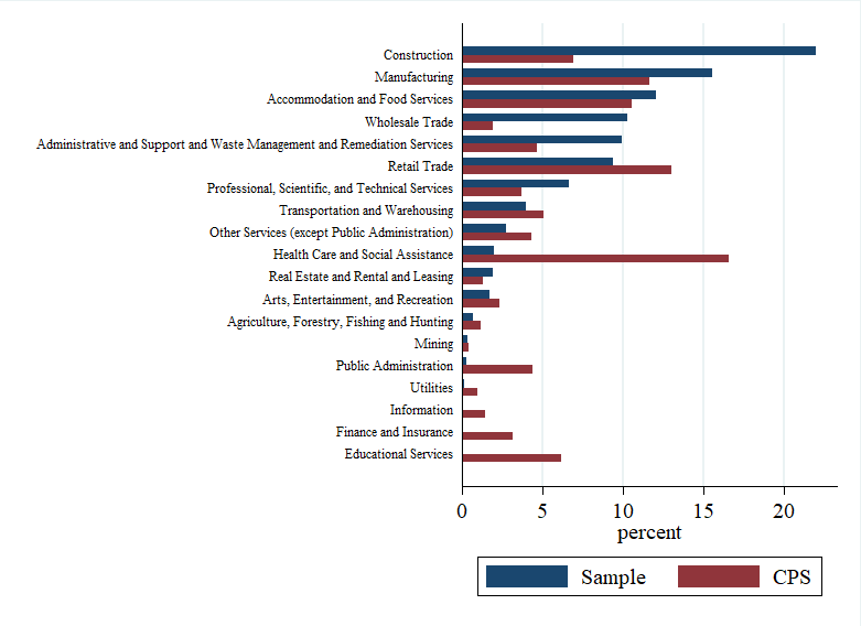
Figure E.6: Industry distribution of estimation sample versus the CPS sample described in Section 3.

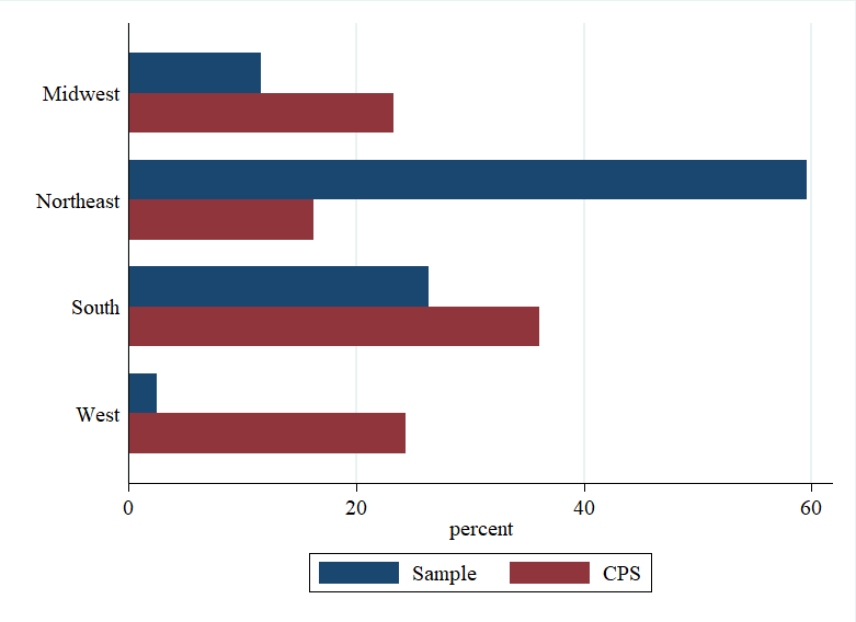
Figure E.7: Geographical distribution of estimation sample versus the CPS sample described in Section 3.

E.2 Additional figures and tables

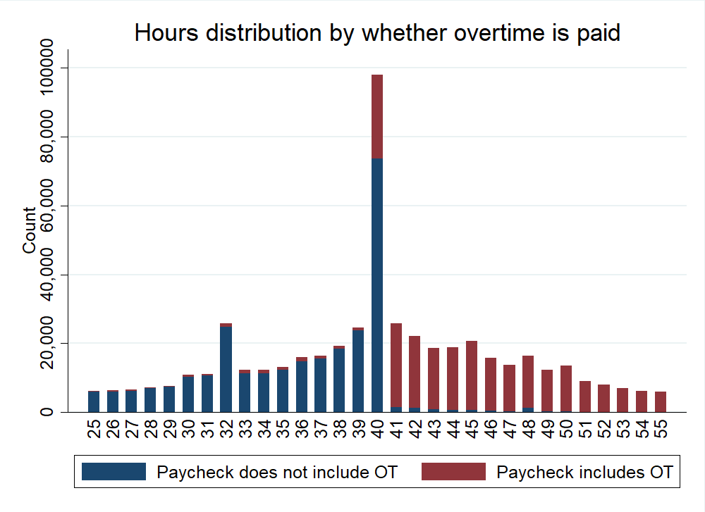
Figure E.8: Histogram of hours worked pooling all paychecks in sample, with one hour bins. Blue mass in the stacks indicate that the paycheck included no overtime pay, while red indicates that the paycheck does include overtime pay. The figure suggests two things: i) compliance with the FLSA overtime mandate is high; and ii) there is little overtime pay voluntarily offered to workers in weeks when they have less than 40 hours of work.

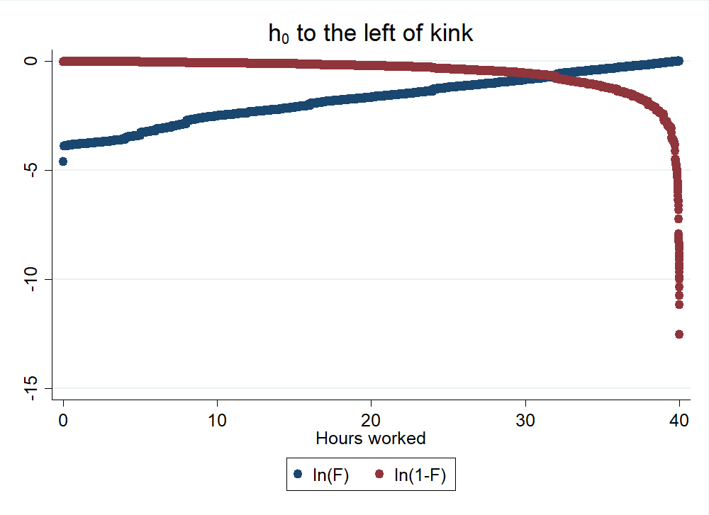
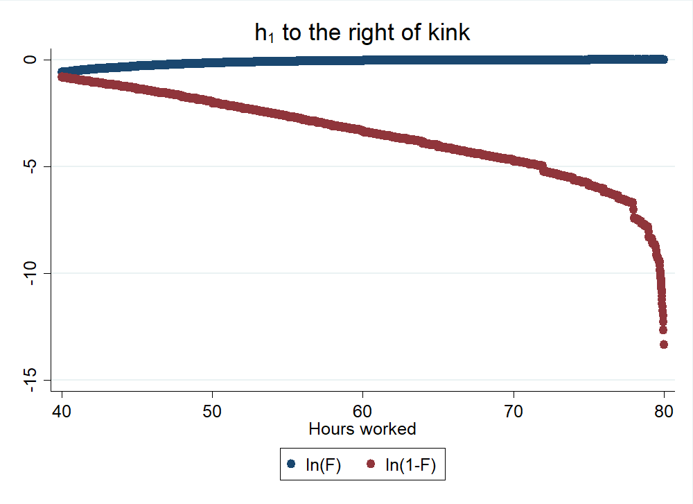
Figure E.9: Validating the assumption of bi-log-concavity away from the kink. The left panel plots estimates of $\ln F_{0}(h)$ and $\ln(1-F_{0}(h))$ for $h<40$, based on the empirical CDF of observed hours worked. Similarly the right panel plots estimates of $\ln F_{1}(h)$ and $\ln(1-F_{1}(h))$ for $h>k$, where I’ve conditioned the sample on $Y_{i}<80$. Bi-log-concavity requires that the four functions plotted be concave globally.

Industry	Avg. OT hours	OT % hours	OT % pay	Industry share
Accommodation and Food Services	2.37	0.06	0.11	0.08
Administrative and Support	5.69	0.13	0.18	0.08
Agriculture, Forestry, Fishing and Hunting	3.76	0.11	0.15	0.00
Arts, Entertainment, and Recreation	3.87	0.10	0.13	0.00
Construction	3.09	0.07	0.10	0.20
Educational Services	1.83	0.05	0.07	0.00
Finance and Insurance	0.31	0.00	0.01	0.00
Health Care and Social Assistance	4.59	0.12	0.12	0.02
Information	1.67	0.04	0.06	0.00
Manufacturing	3.37	0.08	0.11	0.18
Mining	2.26	0.07	0.12	0.00
Other Services	2.61	0.06	0.09	0.02
Professional, Scientific, and Technical Services	2.91	0.07	0.10	0.06
Public Administration	2.36	0.05	0.08	0.00
Real Estate and Rental and Leasing	2.85	0.07	0.09	0.02
Retail Trade	2.83	0.07	0.10	0.08
Transportation and Warehousing	5.24	0.12	0.17	0.04
Utilities	3.80	0.08	0.11	0.00
Wholesale Trade	5.15	0.11	0.14	0.10
Total Sample	3.55	0.08	0.12	0.98

Table E.1: Overtime prevalence by industry in the sample, including average number of OT hours per weekly paycheck, % OT hours among hours worked, % pay for hours work going to OT, and industry share of total hours in sample.

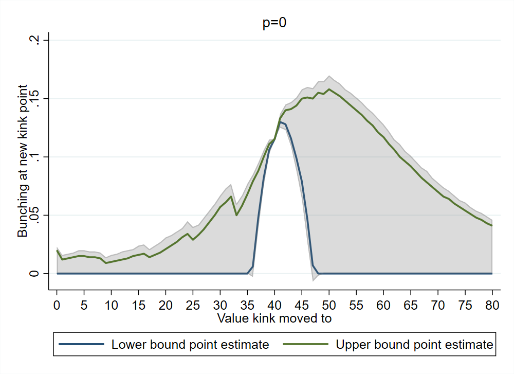
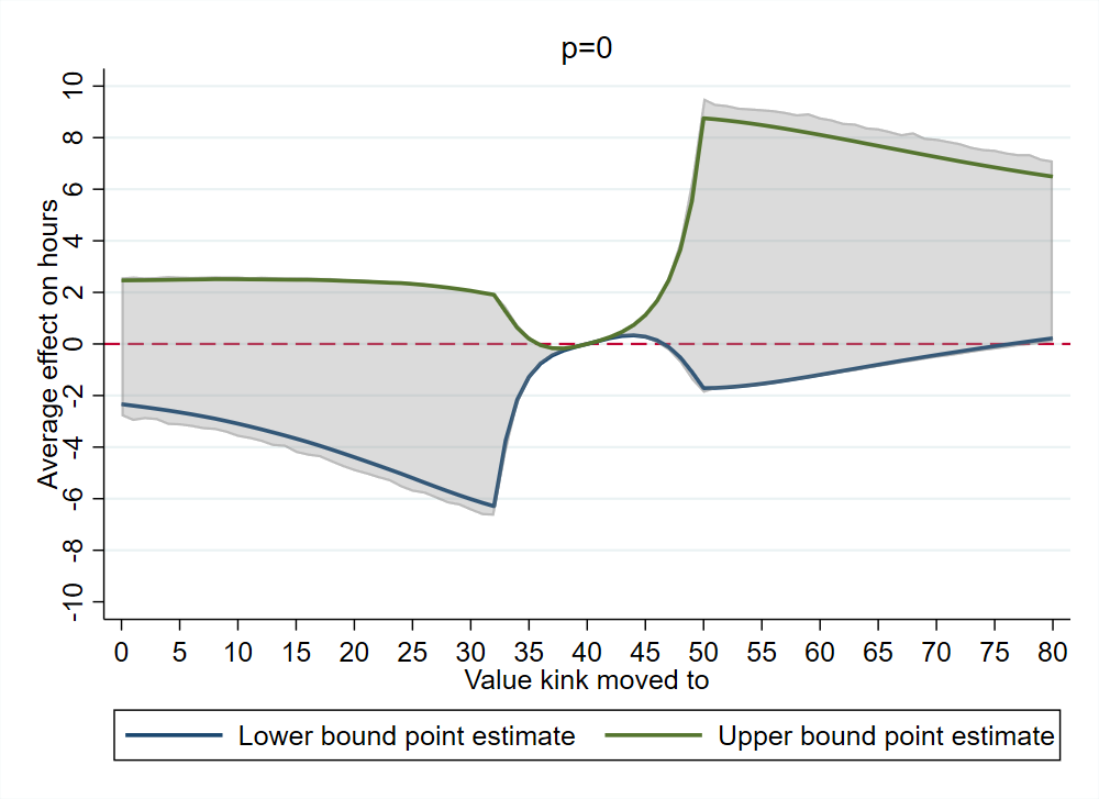
Figure E.10: Estimates of the bunching (left panel) and average effect on hours (right panel) were $k$ changed to any value from 0 to 80, assuming $p=0$. Pointwise bootstrapped 95% confidence intervals, cluster bootstrapped by firm, are shaded gray. Bounds are not informative far from 40. These estimates do not account for adjustment to straight-time wages, so should be viewed as quantifying short-run responses.

Bunching at new kink	Average effect on hours

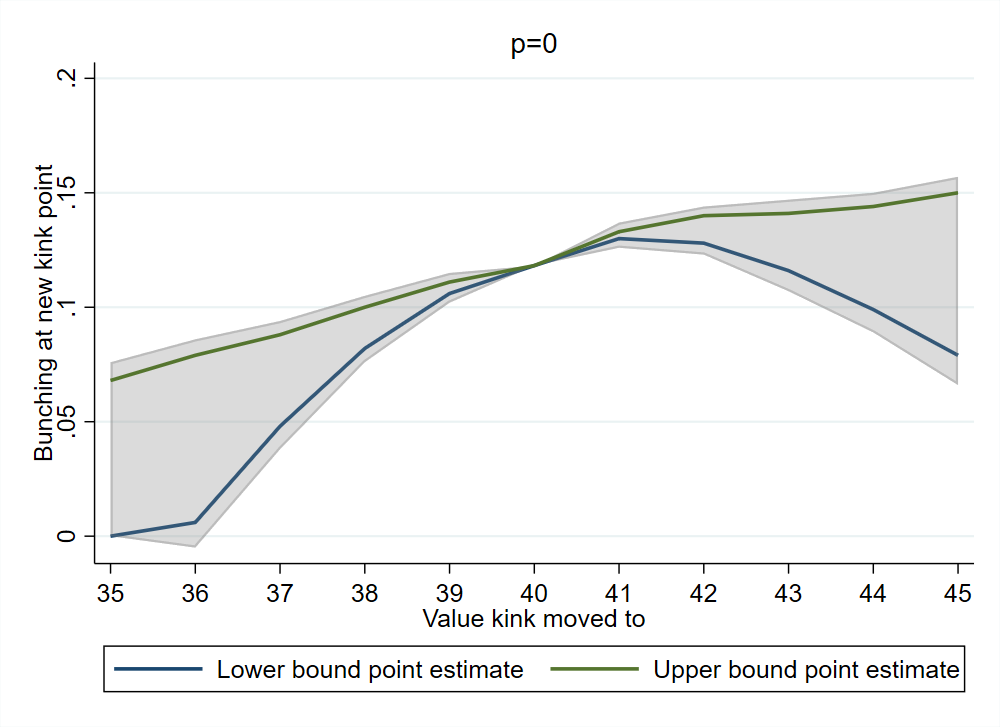
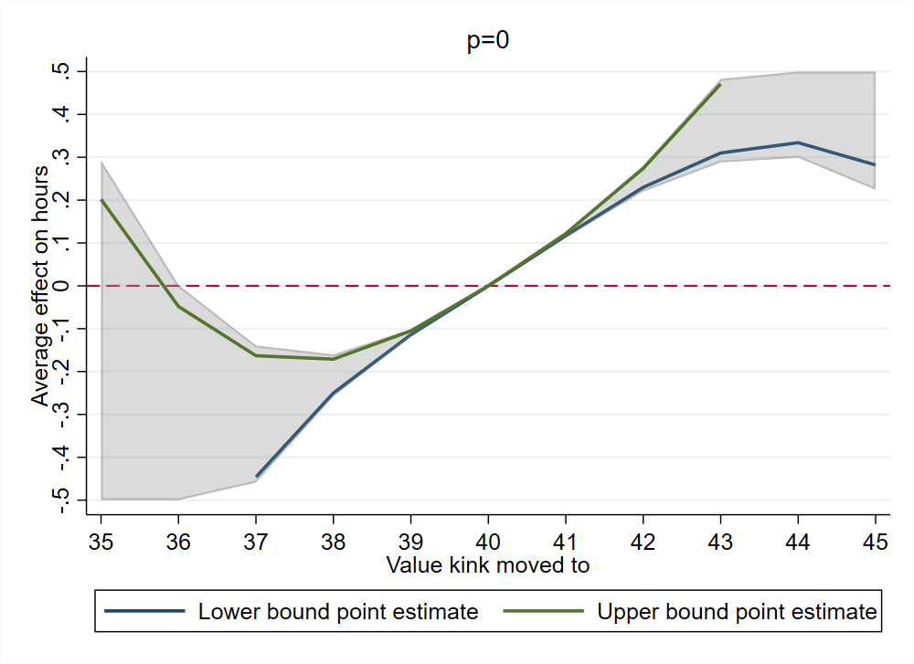
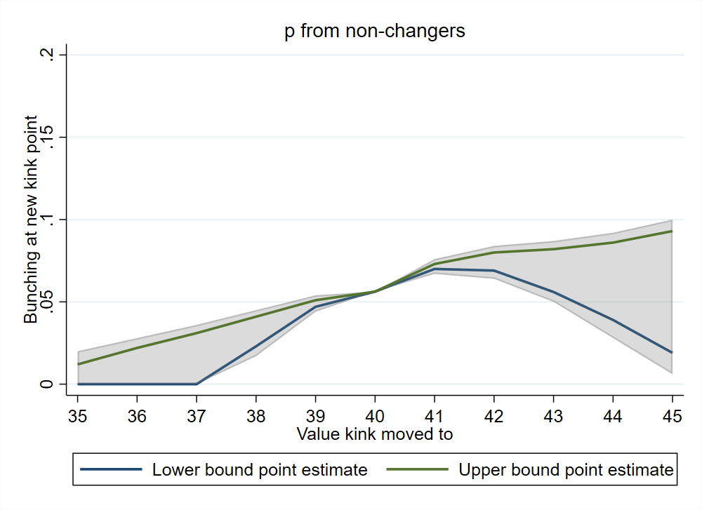
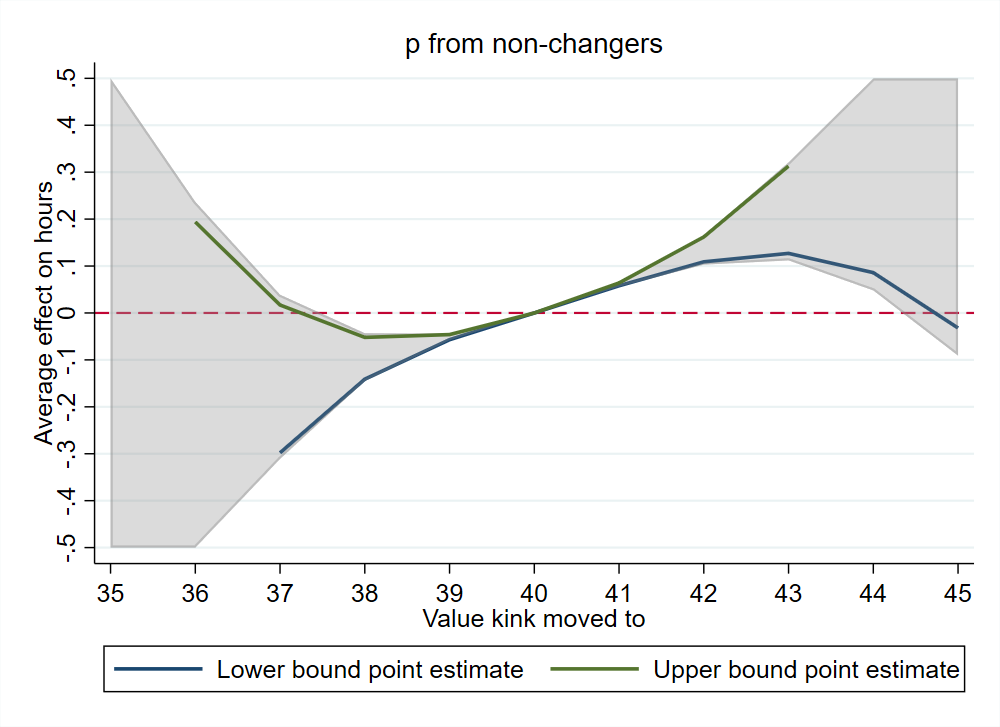
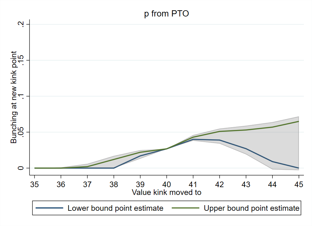
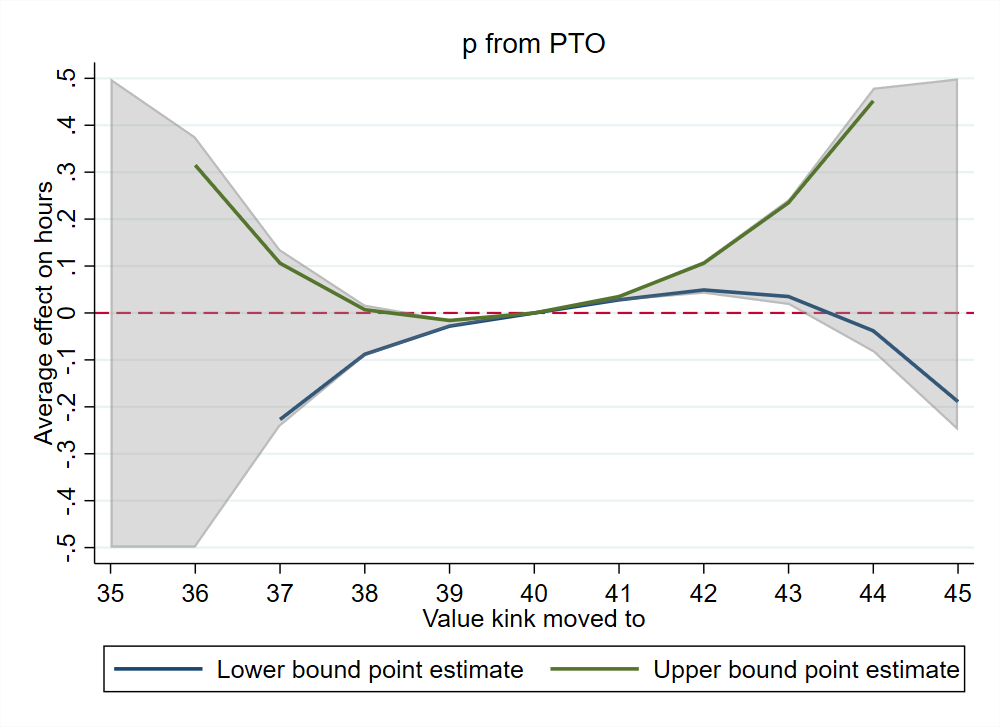
Figure E.11: Bounds for the bunching that would exist at standard hours $k$ if it were changed from 40 (left panel), as well as for the impact on average hours (right panel). Bounds of the effect on hours are clipped to the interval $[-0.5,0.5]$ for visibility. Pointwise bootstrapped 95% confidence intervals, cluster bootstrapped by firm, are shaded gray.

E.3 A test of the [51] model of straight-time wage adjustment

One way to assess the role of the wage rigidity reported in Table 2 is to test directly whether straight-time wages and hours are plausibly related at the weekly level according to Equation (1). Given the kink in Eq. (1), we can perform such a test using the wage and hours reported on each paycheck, while making only weak differentiability assumptions on unobservables for identification.

Suppose that for some subset of units $it$, wages are actively adjusted to the hours they work according to Equation (1), in order to target some total earnings $z_{it}$. Denote the corresponding units by a latent variable $A_{it}=1$. These units may come from workers with limited variation in their schedules in those weeks in which $h_{it}=h^{*}_{i}$ for some typical hours $h^{*}_{i}$ according to which their wages were set by Eq. (1) at hiring. $A_{it}=1$ units might instead have dynamic wages that adjust to week-by-week variation in their hours $h_{it}$. Let $A_{it}=0$ denote units for whom the worker’s wage is determined in some other way. Let $q(h)=P(A_{it}=1|h_{it}=h)$ denote the proportion of these two groups at various points in the hours distribution. An extreme version of the fixed-job model of [51] for example, would have $q(h)=1$ for all $h$.

By the law of iterated expectations and some algebra we have that:

$$\mathbbm{E}\left[\ln w_{it}|h_{it}=h\right] =q(h)\left\{\mathbbm{E}\left[\ln z_{it}|h_{it}=h,A_{it}=1\right]-\ln\left(h+0.5(h-40)\mathbbm{1}(h\geq 40)\right)\right\}$$

$$\hskip 180.67499pt-(1-q(h))\mathbbm{E}\left[\ln w_{it}|h_{it}=h,A_{it}=0\right]$$

The middle term above introduces a kink in the conditional expectation of the log of straight-time wages with respect to hours. If we assume that $\mathbbm{E}\left[\ln z_{it}|h_{it}=h,A_{it}=1\right]$, $\mathbbm{E}\left[\ln w_{it}|h_{it}=h,A_{it}=0\right]$ and $q(h)$ are all continuously differentiable in $h$, then the magnitude of this kink identifies $q(40)$, the proportion of active wage responders local to $h=40$:

$$\lim_{h\downarrow 40}\frac{d}{dh}\mathbbm{E}\left[\ln w_{it}|h_{it}=h\right]-\lim_{h\uparrow 40}\frac{d}{dh}\mathbbm{E}\left[\ln w_{it}|h_{it}=h\right]=-\frac{1}{2}\cdot\frac{q(40)}{40}$$

These continuous differentiability assumptions are reasonable, if wage setting according to Equation (1) is the only force introducing non-smoothness in the relationship between wages and hours at 40. For instance, we assume that production technologies do not have any special features at 40 hours that would cause the distribution of target earnings levels $z_{it}$ among the $A_{it}=1$ units to itself have a kink around $h_{it}=40$.

Figure E.12 reports the results of fitting separate local linear functions to the CEF of log wages on either side of $h=40$. We can reject the hypothesis that the fixed-job model applies to all employees at all times, near $40$. However, the data appear to be consistent with a proportion $q(40)\approx 0.25$ of all paychecks close to 40 hours reflecting an hours/wage relationship governed by Equation (1). This can be rationalized by straight-wages being updated intermittently to reflect expected or anticipated hours, which vary in practice quite a bit between pay periods.

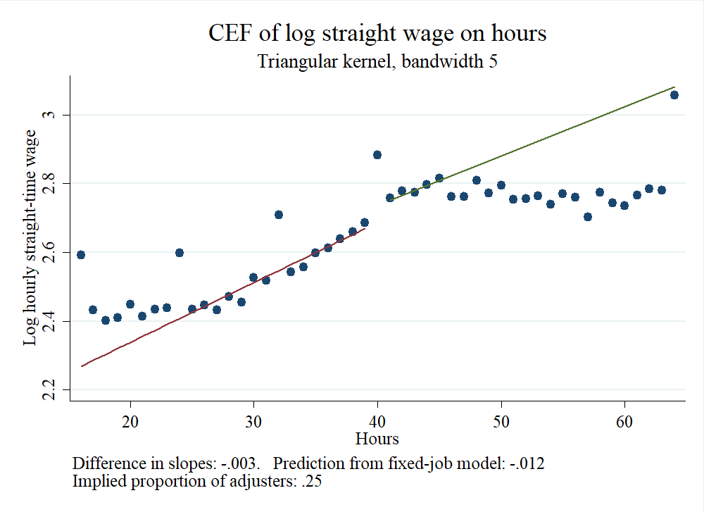
Figure E.12: A test of the fixed-jobs model presented in [51], based on the magnitude of the kink in the conditional expectation of log wages with respect to hours at 40 (see above). Regression lines fit on each side with a uniform kernel within 25 hours of the 40. This figure closely resembles Figure 5 of [5] which uses CPS data for hourly workers.

E.4 Details of the employment effect calculation

Taking my prefered estimate that hourly workers work approximately 1/3 of an hour less per week on average because of the rule, hours per worker are reduced by just under 1%. If we assume the same sized effect occurs for covered salaried workers, and ignore scale effects of the overtime rule on the total number of labor hours in FLSA-eligible jobs, this suggests employment among such jobs is 1% higher than it would be without the overtime premium. This serves as an upper bound, since overall total hours worked may decrease due to overtime regulation.

Following [27], assume that the percentage change in employment decomposes as:

$$\left.\Delta\ln E\right|_{EH}-\eta\cdot\Delta\ln LC\cdot\frac{\eta}{\alpha-\eta}$$ (E.7)

where $\eta$ is constant-output demand elasticity for labor, $\alpha$ is a labor supply elasticity. Following [27] I use $\Delta\ln LC=0.7\%$ based on [22], calibrated assuming that 80% of labor costs come from wages with overtime representing $2\%$ of total hours. $\left.\Delta\ln E\right|_{EH}$ is the quantity implied by my estimates: the percentage change in employment that would occur were the total number of worker-hours $EH$ unchanged. Taking a preferred estimate of the average effect of the FLSA as reported in Table 4 to be about 1/3 of an hour, I use a value of $\left.\Delta\ln E\right|_{EH}=\frac{1/3}{40}\approx 0.9\%$.

			$\eta$
		-0.15	-0.3	-0.5
	0	0.76	0.64	0.50
$\alpha$	0.1	0.80	0.70	0.56
	0.5	0.85	0.79	0.68

Table E.2: Back-of-the-envelope employment effects based on the average reduction in hours estimated via the bunching design and Equation (E.7), as a function of the demand elasticity for labor (rather than capital) $\eta$, and labor supply elasticity $\alpha$. The bold entry reflects “best-guess” values of $\eta$ and $\alpha$.

“Best-guess” values for the other parameters used by [27] are $\eta=-0.3$ and $\alpha=0.1$, based on a review of empirical estimates. This yields $0.17$ percentage points for the substitution term $\eta\cdot\Delta\ln LC\cdot\frac{\eta}{\alpha-\eta}$, suggesting that the effect of the FLSA is attenuated from roughly $0.87$ percentage points to about a $0.70$ percentage point net increase in employment. I assume that the FLSA overtime rule applies to a total of 100 million workers, based on 80 million hourly workers combined with an estimated 20 million covered salary workers [36]. Assuming the same percentage increase in employment applies to hourly workers and covered salary workers, the above estimate corresponds to 700,000 jobs created. Generating a negative overall employment response by assuming higher substitution to capital requires $\eta=-1.25$, well outside of empirical estimates.

Appendix F Additional proofs

F.1 Proof of Propositions 1 and 2

Consider Proposition 1. Item i) in the proof of Lemma 1 establishes that under CHOICE and WARP $Y_{i}=k$ implies $Y_{1i}\leq k\leq Y_{0i}$, since taking contrapositives we have that $(Y_{i}\geq k$ and $Y_{i}\leq k)$ implies $Y_{1i}\leq k\leq Y_{0i}$. We have also seen from item ii) that under CHOICE and CONVEX $Y_{1i}\leq k\leq Y_{0i}$ also implies $Y_{i}=k$, thus $Y_{1i}\leq k\leq Y_{0i}$ and $Y_{i}=k$ are equivalent. Note that by adding $\Delta_{i}=Y_{0i}-Y_{1i}$ to both sides of the inequality $Y_{1i}\leq k$, we have that $Y_{0i}\leq k+\Delta_{i}$. Combining with the other inequality that $Y_{0i}\geq k$, we can thus rewrite the event $Y_{1i}\leq k\leq Y_{0i}$ as $Y_{0i}\in[k,k+\Delta_{i}]$ (or equivalently to $Y_{1i}\in[k-\Delta_{i},k]$). We thus have that $\mathcal{B}\leq P(Y_{0i}\in[k,k+\Delta])$ under CHOICE and WARP, and that $\mathcal{B}=P(Y_{i}=k)=P(Y_{1i}\leq k\leq Y_{0i})$ under CHOICE and CONVEX.

Now consider Proposition 2. By item i) in the proof of Proposition 1, we have that under WARP and CHOICE $Y_{0i}\leq k\implies Y_{i}=Y_{0i}$. Thus, for any $\delta>0$ and $y<k$: $Y_{0i}\in[y-\delta,y]$ implies that $Y_{i}\in[y-\delta,y]$ and hence $P(Y_{0i}\in[y-\delta,y])\leq P(Y_{i}\in[y-\delta,y])$. This implies that $f_{0}(y)-f(y)=\lim_{\delta\downarrow 0}\frac{P(Y_{0i}\in[y-\delta,y])-P(Y_{i}\in[y-\delta,y])}{\delta}\leq 0$, i.e. that $f(y)\geq f_{0}(y)$. An analogous argument holds for $Y_{1}$, where we consider the event $Y_{1i}\in[y,y+\delta]$ any $y>k$. Under CONVEX instead of WARP, the inequalities are all equalities, by Lemma 1.

F.2 Proof of Lemma 2

Let $\Delta^{k}_{i}(\rho,\rho^{\prime}):=Y_{i}(\rho,k)-Y_{i}(\rho^{\prime},k)$ for any $\rho,\rho^{\prime}\in[\rho_{0},\rho_{1}]$ and value of $k$.

Assumption (SMOOTH (regularity conditions)).

The following hold:

1. $P(\Delta^{k}_{i}(\rho,\rho^{\prime})\leq\Delta,Y_{i}(\rho,k)\leq y)$ is twice continuously differentiable at all $(\Delta,y)\neq(0,k^{*})$, for any $\rho,\rho^{\prime}\in[\rho_{0},\rho_{1}]$ and $k$.

2. $Y_{i}(\rho,k)=Y(\rho,k,\epsilon_{i})$, where $\epsilon_{i}$ has compact support $E\subset\mathbbm{R}^{m}$ for some $m$. $Y(\cdot,k,\cdot)$ is continuously differentiable on all of $[\rho_{0},\rho_{1}]\times E$, for every $k$.

3. there possibly exists a set $\mathcal{K}^{*}\subset E$ such that $Y(\rho,k,\epsilon)=k^{*}$ for all $\rho\in[\rho_{0},\rho_{1}]$ and $\epsilon\in\mathcal{K}^{*}$. The quantity $\mathbbm{E}\left[\left.\frac{\partial Y_{i}(\rho,k)}{\partial\rho}\right|Y_{i}(\rho,k)=y,\epsilon_{i}\notin\mathcal{K}^{*}\right]$ is continuously differentiable in $y$ for all $y$ including $k^{*}$.

In the remainder of this proof I keep $k$ be implicit in the functions $Y_{i}(\rho,k)$ and $\Delta^{k}_{i}(\rho,\rho^{\prime})$, as it will remained fixed. Item 1 of SMOOTH excludes the point $(0,k^{*})$ on the basis that we may expect point masses at $Y_{i}(\rho)=k^{*}$, as in the overtime setting. Following Section 4, item 3 imposes that all such “counterfactual bunchers” have zero treatment effects, while also introducing a further condition that will be used later in Lemma 3. Let $K_{i}^{*}$ be an indicator for $\epsilon_{i}\in\mathcal{K}^{*}$ and denote $p=P(K_{i}^{*}=1)$. Item 1 implies that the density $f_{\Delta(\rho,\rho^{\prime}),Y(\rho)}(\Delta,y)$ is continuous in $y$ whenever $y\neq k^{*}$ or $\Delta\neq 0$, so I define $f_{\Delta(\rho,\rho^{\prime}),Y(\rho)}(\Delta,k^{*})=\lim_{y\rightarrow k^{*}}f_{\Delta(\rho,\rho^{\prime}),Y(\rho)}(\Delta,y)$ for any $\rho,\rho^{\prime}$ and $\Delta$. Similarly, we can define the marginal density $f_{\rho}(y)$ of $Y_{i}(\rho$) at $k^{*}$ to be $\lim_{y\rightarrow k^{*}}f_{\rho}(y)$ for any $\rho$.

By item 1 of Assumption SMOOTH, the marginal $F_{\rho}(y):=P(Y_{i}(\rho)\leq y)$ is differentiable away from $y=k$ with derivative $f_{\rho}(y)$. From the proof of Theorem 1 it follows that $\mathcal{B}\leq F_{\rho_{1}}(k)-F_{\rho_{0}}(k)+p(k)$ with equality under CONVEX, and thus:

$$\mathcal{B}-p(k) \leq F_{\rho_{1}}(k)-F_{\rho_{0}}(k)=\int_{\rho_{0}}^{\rho_{1}}\frac{d}{d\rho}F_{\rho}(k)d\rho=\int_{\rho_{0}}^{\rho_{1}}\lim_{\delta\downarrow 0}\frac{F_{\rho+\delta}(k)-F_{\rho}(k)}{\delta}d\rho$$

$$=\int_{\rho_{1}}^{\rho_{0}}\lim_{\delta\downarrow 0}\frac{P(Y_{i}(\rho+\delta)\leq k\leq Y_{i}(\rho))-p(k)}{\delta}d\rho=\int_{\rho_{1}}^{\rho_{0}}f_{\rho}(k)\mathbbm{E}\left[\left.-\frac{Y_{i}(\rho)}{d\rho}\right|Y_{i}(\rho)=k\right]d\rho$$

where the third equality applies the identity $1=P(Y_{0i}\leq k)+P(Y_{i}(\rho)\leq k\leq Y_{i}(\rho+\delta))+P(Y_{1i}>k)$ under CHOICE and WARP (this follows from item i) of the proof of Lemma 1) to the pair of choice constraints $B(\rho)$ and $B(\rho+\delta)$, noting that $P(Y_{i}(\rho)<k)=F_{\rho}(k)-p(k)$. The final equality uses Lemma SMALL.

F.3 Proof of Lemma SMALL

Throughout this proof we let $f_{W}$ denote the density of a generic random variable or random vector $W_{i}$, if it exists. Write $\Delta_{i}(\rho,\rho^{\prime})=\Delta_{i}(\rho_{,}\rho^{\prime},\epsilon_{i})$ where $\Delta_{i}(\rho,\rho^{\prime},\epsilon):=Y(\rho,\epsilon)-Y(\rho^{\prime},\epsilon)$.

$$\lim_{\rho^{\prime}\downarrow\rho}\frac{P(Y_{i}(\rho)\leq k\leq Y_{i}(\rho^{\prime}))-p(k)}{\rho^{\prime}-\rho} = \lim_{\rho^{\prime}\downarrow\rho}\frac{P(Y_{i}(\rho)\in[k,k+\Delta(\rho,\rho^{\prime})_{i}])-p(k)}{\rho^{\prime}-\rho}$$

$$= \lim_{\rho^{\prime}\downarrow\rho}\frac{P(Y_{i}(\rho)\in(k,k+\Delta(\rho,\rho^{\prime})_{i}])}{\rho^{\prime}-\rho}$$

$$= \lim_{\rho^{\prime}\downarrow\rho}\frac{1}{\rho^{\prime}-\rho}\int_{0}^{\infty}d\Delta\int_{k}^{k+\Delta}dy\cdot f_{\Delta(\rho,\rho^{\prime}),Y(\rho)}(\Delta,y)$$

$$= \lim_{\rho^{\prime}\downarrow\rho}\int_{0}^{\infty}d\Delta\int_{k}^{k+\Delta}dy\cdot\frac{f_{\Delta(\rho,\rho^{\prime}),Y(\rho)}(\Delta,k)+(y-k)r_{\Delta(\rho,\rho^{\prime}),Y(\rho)}(\Delta,k,y)}{\rho^{\prime}-\rho}$$

where we have used that by item 1 the joint density of $\Delta_{i}(\rho,\rho^{\prime})$ and $Y_{i}(\rho)$ exists for any $\rho,\rho^{\prime}$ and is differentiable and $r_{\Delta(\rho,\rho^{\prime}),Y(\rho)}$ is a first-order Taylor remainder term satisfying

$$\lim_{y\downarrow k}|r_{\Delta(\rho,\rho^{\prime}),Y(\rho)}(\Delta,y)|=|r_{\Delta(\rho,\rho^{\prime}),Y(\rho)}(\Delta,k)|=0$$

for any $\Delta$.

I now show that the whole term corresponding to this remainder is zero. First, note that:

$$\left|\lim_{\rho^{\prime}\downarrow\rho}\int_{0}^{\infty}d\Delta\int_{k}^{k+\Delta}dy\cdot\frac{(y-k)r_{\Delta_{i}(\rho,\rho^{\prime}),Y_{i}(\rho)}(\Delta,y)}{\rho^{\prime}-\rho}\right| =\lim_{\rho^{\prime}\downarrow\rho}\left|\int_{0}^{\infty}d\Delta\int_{k}^{k+\Delta}dy\cdot\frac{(y-k)r_{\Delta_{i}(\rho,\rho^{\prime}),Y_{i}(\rho)}(\Delta,y)}{\rho^{\prime}-\rho}\right|$$

$$\leq\lim_{\rho^{\prime}\downarrow\rho}\int_{0}^{\infty}d\Delta\int_{k}^{k+\Delta}dy\cdot\left|\frac{(y-k)r_{\Delta_{i}(\rho,\rho^{\prime}),Y_{i}(\rho)}(\Delta,y)}{\rho^{\prime}-\rho}\right|$$

$$\leq\lim_{\rho^{\prime}\downarrow\rho}\int_{0}^{\infty}d\Delta\frac{\Delta}{\rho^{\prime}-\rho}\int_{k}^{k+\Delta}dy\cdot\left|r_{\Delta_{i}(\rho,\rho^{\prime}),Y_{i}(\rho)}(\Delta,y)\right|$$

where I’ve used continuity of the absolute value function and the Minkowski inequality. Define $\xi(\rho,\rho^{\prime})=\sup_{\epsilon\in E}\Delta(\rho,\rho^{\prime},\epsilon)$. The strategy will be show that $\lim_{\rho^{\prime}\downarrow\rho}\xi(\rho,\rho^{\prime})=0$, and then since $r_{\Delta_{i}(\rho,\rho^{\prime}),Y_{i}(\rho)}(\Delta,y)=0$ for any $\Delta>\xi(\rho,\rho^{\prime})$ and all $y$ (since the marginal density $f_{\Delta(\rho,\rho^{\prime})}(\Delta)$ would be zero for such $\Delta$). With $\xi(\rho,\rho^{\prime})$ so-defined:

RHS of above $$\leq \lim_{\rho^{\prime}\downarrow\rho}\int_{0}^{\xi(\rho,\rho^{\prime})}d\Delta\frac{\xi(\rho,\rho^{\prime})}{\rho^{\prime}-\rho}\int_{k}^{k+\xi(\rho,\rho^{\prime})}dy\cdot\left|r_{\Delta_{i}(\rho,\rho^{\prime}),Y_{i}(\rho)}(\Delta,y)\right|$$ (F.9)

$$= \lim_{\rho^{\prime}\downarrow\rho}\frac{\xi(\rho,\rho^{\prime})}{\rho^{\prime}-\rho}\cdot\lim_{\rho^{\prime}\downarrow\rho}\int_{0}^{\xi(\rho,\rho^{\prime})}d\Delta\int_{0}^{\xi(\rho,\rho^{\prime})}dy\cdot\left|r_{\Delta_{i}(\rho,\rho^{\prime}),Y_{i}(\rho)}(\Delta,k+y)\right|$$

where in the second step I have assumed that each limit exists (this will be demonstrated below). Let us first consider the inner integral of the above: $\int_{k}^{k+\xi(\rho,\rho^{\prime})}dy\cdot\left|r_{\Delta_{i}(\rho,\rho^{\prime}),Y_{i}(\rho)}(\Delta,y)\right|$, for any $\Delta$. Supposing that $\lim_{\rho^{\prime}\downarrow\rho}\xi(\rho,\rho^{\prime})=0$, it follows that this inner integral evaluates to zero, by the Leibniz rule and using that $r_{\Delta_{i}(\rho,\rho^{\prime}),Y_{i}(\rho)}(\Delta,k)=0$. Thus the entire second limit is equal to zero.

Now I prove that $\lim_{\rho^{\prime}\downarrow\rho}\xi(\rho,\rho^{\prime})=0$ and that $\lim_{\rho^{\prime}\downarrow\rho}\frac{\xi(\rho,\rho^{\prime})}{\rho^{\prime}-\rho}$ exists. First, note that continuous differentiability of $Y(\rho,\epsilon_{i})$ implies $Y_{i}(\rho)$ is continuous for each $i$ so $\lim_{\rho^{\prime}\downarrow\rho}\Delta_{i}(\rho,\rho^{\prime})=0$ point-wise in $\epsilon$. We seek to turn this point-wise convergence into uniform convergence over $\epsilon$, i.e. that $\lim_{\rho^{\prime}\downarrow\rho}\sup_{\epsilon\in E}\Delta(\rho,\rho^{\prime},\epsilon)=\sup_{\epsilon\in E}\lim_{\rho^{\prime}\downarrow\rho}\Delta(\rho,\rho^{\prime},\epsilon)=\sup_{\epsilon\in E}0=0$. The strategy will be to use equicontinuity of the sequence and compactness of $E$. Consider any such sequence $\rho_{n}\stackrel{{\scriptstyle n}}{{\rightarrow}}\rho$ from above, and let $f_{n}(\epsilon):=Y(\rho,\epsilon)-Y(\rho_{n},\epsilon)$ and $f(\epsilon)=\lim_{n\rightarrow\infty}f_{n}(\epsilon)=0$. Equicontinuity of the sequence $f_{n}(\epsilon)$ says that for any $\epsilon,\epsilon^{\prime}\in E$ and $e>0$, there exists a $\delta>0$ such that $||\epsilon-\epsilon^{\prime}||<\delta\implies|f_{n}(\epsilon)-f_{n}(\epsilon^{\prime})|<e$.

This follows from continuous differentiability of $Y(\rho,\epsilon)$. Let $M=\sup_{\rho\in[\rho_{0},\rho_{1}],\epsilon\in E}|\nabla_{\rho,\epsilon}Y(\rho,\epsilon)|$. $M$ exists and is finite given continuity of the gradient and compactness of $[\rho_{0},\rho_{1}]\times E$. Then, for any two points $\epsilon,\epsilon^{\prime}\in E$ and any $\rho\in[\rho_{0},\rho_{1}]$:

$$|Y(\rho,\epsilon)-Y(\rho,\epsilon^{\prime})|=\left|\int_{\epsilon^{\prime}}^{\epsilon}\nabla_{\epsilon}Y(\rho,\epsilon)\cdot\mathbf{d}\epsilon\right|\leq\int_{\epsilon^{\prime}}^{\epsilon}\left|\nabla_{\epsilon}Y(\rho,\epsilon)\cdot\mathbf{d}\epsilon\right|\leq M\int_{\epsilon^{\prime}}^{\epsilon}\left|\left|\mathbf{d}\epsilon\right|\right|\leq M||\epsilon-\epsilon^{\prime}||$$

where $\mathbf{d}\epsilon$ is any path from $\epsilon$ to $\epsilon^{\prime}$ and I have used the definition of $M$ and Cauchy-Schwarz in the second inequality. The existence of a uniform Lipschitz constant $M$ for $Y(\rho,\epsilon)$ implies a uniform equicontinuity of $Y(\rho,\epsilon)$ of the form that for any $e>0$ and $\epsilon,\epsilon^{\prime}\in E$, there exists a $\delta>0$ such that $||\epsilon-\epsilon^{\prime}||<\delta\implies\sup_{\rho\in[\rho_{0},\rho_{1}]}|Y(\rho,\epsilon)-Y(\rho,\epsilon^{\prime})|<e/2$, since we can simply take $\delta=e/(2M)$. This in turn implies that whenever $||\epsilon-\epsilon^{\prime}||<\delta$:

$$|Y(\rho,\epsilon)-Y(\rho_{n},\epsilon)-\left\{Y(\rho,\epsilon^{\prime})-Y(\rho_{n},\epsilon^{\prime})\right\}| =|Y(\rho,\epsilon)-Y(\rho,\epsilon^{\prime})-\left\{Y(\rho_{n},\epsilon)-Y(\rho_{n},\epsilon^{\prime})\right\}|$$

$$\leq|Y(\rho,\epsilon)-Y(\rho,\epsilon^{\prime})|+|Y(\rho_{n},\epsilon)-Y(\rho_{n},\epsilon^{\prime})|\leq e,$$

our desired result. Together with compactness of $E$, equicontinuity implies that $\lim_{n\rightarrow\infty}\sup_{\epsilon\in E}f_{n}(\epsilon)=\sup_{\epsilon\in E}\lim_{n\rightarrow\infty}f_{n}(\epsilon)=0$.

We apply an analogous argument for $\lim_{\rho^{\prime}\downarrow\rho}\frac{\xi(\rho,\rho^{\prime})}{\rho^{\prime}-\rho}$, where now $f_{n}(\epsilon)=\frac{Y(\rho,\epsilon)-Y(\rho_{n},\epsilon)}{\rho_{n}-\rho}$. For this case it’s easier to work directly with the function $\frac{Y(\rho,\epsilon)-Y(\rho_{n},\epsilon)}{\rho_{n}-\rho}$, showing that it is Lipschitz in deviations of $\epsilon$ uniformly over $n\in\mathbbm{N},\epsilon\in E$.

$$\left|\frac{Y(\rho,\epsilon)-Y(\rho_{n},\epsilon)}{\rho_{n}-\rho}-\frac{Y(\rho,\epsilon^{\prime})-Y(\rho_{n},\epsilon^{\prime})}{\rho_{n}-\rho}\right| =\frac{1}{\rho_{n}-\rho}\left|\int_{\epsilon^{\prime}}^{\epsilon}\nabla_{\epsilon}Y(\rho,\epsilon)\cdot\mathbf{d}\epsilon-\int_{\epsilon^{\prime}}^{\epsilon}\nabla_{\epsilon}Y(\rho_{n},\epsilon)\cdot\mathbf{d}\epsilon\right|$$

$$\leq\frac{1}{\rho_{n}-\rho}\left(\left|\int_{\epsilon^{\prime}}^{\epsilon}\nabla_{\epsilon}Y(\rho,\epsilon)\cdot\mathbf{d}\epsilon\right|+\left|\int_{\epsilon^{\prime}}^{\epsilon}\nabla_{\epsilon}Y(\rho_{n},\epsilon)\cdot\mathbf{d}\epsilon\right|\right)$$

$$\leq\frac{2M}{\rho_{n}-\rho}\int_{\epsilon^{\prime}}^{\epsilon}\left|\left|\mathbf{d}\epsilon\right|\right|\leq\frac{2M}{\rho_{n}-\rho}||\epsilon-\epsilon^{\prime}||$$

This implies equicontinuity of $\frac{Y(\rho,\epsilon)-Y(\rho_{n},\epsilon)}{\rho_{n}-\rho}$with the choice $\delta=e(\rho_{n}-\rho)/(2M)$. As before, equicontinuity and compactness of $E$ allow us to interchange the limit and the supremum, and thus:

$$\lim_{n\rightarrow\infty}\frac{\xi(\rho,\rho_{n})}{\rho_{n}-\rho} =\lim_{n\rightarrow\infty}\frac{\sup_{\epsilon\in E}\left\{Y(\rho,\epsilon)-Y(\rho_{n},\epsilon)\right\}}{\rho_{n}-\rho}=\lim_{n\rightarrow\infty}\sup_{\epsilon\in E}\frac{Y(\rho,\epsilon)-Y(\rho_{n},\epsilon)}{\rho_{n}-\rho}$$

$$=\sup_{\epsilon\in E}\lim_{n\rightarrow\infty}\frac{Y(\rho,\epsilon)-Y(\rho_{n},\epsilon)}{\rho_{n}-\rho}=\sup_{\epsilon\in E}\frac{\partial Y(\rho,\epsilon)}{\partial\rho}:=M^{\prime}<\infty$$

where finiteness of $M^{\prime}$ follows from it being defined as the supremum of a continuous function over a compact set. This establishes that the first limit in Eq. (F.9) exists and is finite, completing the proof that it evaluates to zero.

Given that the second term in Eq. (LABEL:tayloreq) is zero, we can simplify the remaining term as:

$$\lim_{\rho^{\prime}\downarrow\rho} \frac{P(Y_{i}(\rho)\leq k\leq Y_{i}(\rho^{\prime}))-p(k)}{\rho^{\prime}-\rho}=\lim_{\rho^{\prime}\downarrow\rho}\frac{1}{\rho^{\prime}-\rho}\int_{0}^{\infty}f_{\Delta(\rho,\rho^{\prime}),Y(\rho)}(\Delta,k)\Delta d\Delta$$

$$=f_{\rho}(k)\lim_{\rho^{\prime}\downarrow\rho}\frac{1}{\rho^{\prime}-\rho}P(\Delta_{i}(\rho,\rho^{\prime})\geq 0|Y_{i}(\rho)=k)\cdot\mathbbm{E}\left[\Delta_{i}(\rho,\rho^{\prime})|Y_{i}(\rho)=k,\Delta_{i}(\rho,\rho^{\prime})\geq 0\right]$$

$$=f_{\rho}(k)(k)\lim_{\rho^{\prime}\downarrow\rho}\frac{1}{\rho^{\prime}-\rho}\mathbbm{E}\left[\Delta_{i}(\rho,\rho^{\prime})|Y_{i}(\rho)=k,\Delta_{i}(\rho,\rho^{\prime})\right]=f_{\rho}(k)(k)\mathbbm{E}\left[\left.\lim_{\rho^{\prime}\downarrow\rho}\frac{\Delta_{i}(\rho,\rho^{\prime})}{\rho^{\prime}-\rho}\right|Y_{i}(\rho)=k\right]$$

$$=f_{\rho}(k)\mathbbm{E}\left[\left.-\frac{Y_{i}(\rho)}{d\rho}\right|Y_{i}(\rho)=k\right]$$

where I have used that treatment effects must be positive at the kink (see Lemma POS in Appendix LABEL:hetero) and then the dominated convergence theorem. To see that we may use it, note that $\frac{dY_{i}(\rho)}{d\rho}=\frac{\partial Y(\rho,\epsilon_{i})}{\partial\rho}<M$ uniformly over all $\epsilon_{i}\in E$, and $\mathbbm{E}\left[\left.M\right|Y_{i}(\rho)=k\right]=M<\infty$.

References

- [1] Anthony Barkume “The Structure of Labor Costs with Overtime Work in U.S. Jobs” In Industrial and Labor Relations Review 64.1, 2010
- [2] R.E. Barlow, F. Proschan and L.C. Hunter “Mathematical Theory of Reliability”, Classics in Applied Mathematics Society for IndustrialApplied Mathematics, 1996 URL: https://books.google.ca/books?id=tO\_ISpJo2VQC
- [3] Marinho Bertanha, Andrew H Mccallum and Nathan Seegert “Better Bunching , Nicer Notching” In SSRN Working Paper, 2020
- [4] Michael Carlos Best, Anne Brockmeyer, Henrik Jacobsen Kleven, Johannes Spinnewijn and Mazhar Waseem “Production vs Revenue Efficiency With Limited Tax Capacity: Theory and Evidence From Pakistan” In Journal of Political Economy 123.6, 2015, pp. 48
- [5] Alexander Bick, Adam Blandin and Richard Rogerson “Hours and Wages” In The Quarterly Journal of Economics (forthcoming), 2022
- [6] John L. Bishow “A Look at Supplemental Pay: Overtime Pay, Bonuses, and Shift Differentials” Publisher: Bureau of Labor Statistics, U.S. Department of Labor In Monthly Labor Review, 2009 URL: https://www.jstor.org/stable/monthlylaborrev.2009.03.038
- [7] Henry W. Block, Thomas H. Savits and Harshinder Singh “The Reversed Hazard Rate Function” In Probability in the Engineering and Informational Sciences 12.1 Cambridge University Press, 1998, pp. 69–90 DOI: 10.1017/S0269964800005064
- [8] Soren Blomquist, Anil Kumar, Che-Yuan Liang and Whitney Newey “Individual heterogeneity, nonlinear budget sets and taxable income” In The Institute for Fiscal Studies Working Paper CWP21/15, 2015
- [9] Soren Blomquist, Anil Kumar, Che-Yuan Liang and Whitney Newey “On Bunching and Identification of the Taxable Income Elasticity” In Journal of Political Economy 129.8, 2021
- [10] Sören Blomquist, Whitney Newey, Anil Kumar and Che-Yuan Liang “On Bunching and Identification of the Taxable Income Elasticity”, Working Paper Series 24136, 2017 DOI: 10.3386/w24136
- [11] F. P. R. Brechling “The Relationship Between Output and Employment in British Manufacturing Industries” In The Review of Economic Studies 32.3, 1965, pp. 187 DOI: 10.2307/2295824
- [12] Charles Brown and Daniel S Hamermesh “Wages and Hours Laws: what do we know? what can be done?” In The Russell Sage Foundation Journal of the Social Sciences 5.5, 2019, pp. 68–87
- [13] Kenneth Burdett and Dale T. Mortensen “Wage Differentials, Employer Size, and Unemployment” In International Economic Review 39.2, 1998, pp. 257 DOI: 10.2307/2527292
- [14] Bureau of Labor Statistics “National Compensation Survey (Restricted-Use Microdata)”, 2020
- [15] Pierre Cahuc and André Zylberberg “Labor economics” Cambridge, Mass.: MIT Press, 2014
- [16] Matias D Cattaneo, Michael Jansson and Xinwei Ma “Simple Local Polynomial Density Estimators” In Journal of the American Statistical Association 115.531, 2020, pp. 1449–1455
- [17] Victor Chernozhukov and Christian Hansen “An IV Model of Quantile Treatment Effects” In Econometrica 73.1, 2005, pp. 245–261
- [18] Raj Chetty, John N Friedman, Tore Olsen and Luigi Pistaferri “Adjustment Costs, Firm Responses, and Micro vs. Macro Labor Supply Elasticities: Evidence from Danish Tax Records.” In Quarterly Journal of Economics 126.2, 2011, pp. 749–804 DOI: 10.1093/qje/qjr013
- [19] Dora L Costa “Hours of Work and the Fair Labor Standards Act: A Study of Retail and Wholesale Trade, 1938–1950” In Industrial and Labor Relations Review, 2000, pp. 17
- [20] Arindrajit Dube, Alan Manning and Suresh Naidu “Monopsony, Misoptimization, and Round Number Bunching in the Wage Distribution” In NBER Working Paper w24991, 2020
- [21] Lutz Dümbgen, Petro Kolesnyk and Ralf A. Wilke “Bi-log-concave distribution functions” In Journal of Statistical Planning and Inference 184, 2017, pp. 1–17 DOI: 10.1016/j.jspi.2016.10.005
- [22] Ronald Ehrenberg and Paul Schumann “Longer hours or more jobs? : an investigation of amending hours legislation to create employment” New York State School of IndustrialLabor Relations, Cornell University, 1982
- [23] Ronald G Ehrenberg “The Impact of the Overtime Premium on Employment and Hours in U . S . Industry” In Economic Inquiry 9.2, 1971
- [24] Liran Einav, Amy Finkelstein and Paul Schrimpf “Bunching at the kink: Implications for spending responses to health insurance contracts” In Journal of Public Economics 146, 2017, pp. 27–40
- [25] John Grigsby, Erik Hurst and Ahu Yildirmaz “Aggregate Nominal Wage Adjustments: New Evidence from Administrative Payroll Data”, 2021, pp. 428–71
- [26] Rameshwar D. Gupta and Asok K. Nanda “Some results on reversed hazard rate” In Communications in Statistics - Theory and Methods 30.11 Taylor & Francis, 2001, pp. 2447–2457 DOI: 10.1081/STA-100107697
- [27] Daniel S Hamermesh “Labor demand” Princeton, NJ: Princeton Univ. Press, 1993
- [28] Daniel S Hamermesh and Stephen J Trejo “The Demand for Hours of Labor : Direct Evidence from California” In The Review of Economics and Statistics 82.1, 2000, pp. 38–47
- [29] Robert A Hart “The economics of overtime working” Cambridge, UK: Cambridge University Press, 2004
- [30] Jonas Hjort, Xuan Li and Heather Sarsons “Across-Country Wage Compression in Multinationals” In NBER Working Paper w26788, 2020
- [31] Guido W Imbens and Charles F Manski “Confidence Intervals for Partially Identified Parameters” In Econometrica 72, 2004, pp. 14
- [32] John H. Johnson “The Impact of Federal Overtime Legislation on Public Sector Labor Markets” In Journal of Labor Economics 21.1, 2003, pp. 43–69 DOI: 10.1086/344123
- [33] Maximilian Kasy “Who wins, who loses? Identification of the welfare impact of changing wages” In Journal of Econometrics 226.1, 2022, pp. 1–26
- [34] Julian Keilson “Log-Concavity and Log-Convexity in Passage Time Densities of Diffusion and Birth-Death Processes” In Journal of Applied Probability 8.2 Applied Probability Trust, 1971, pp. 391–398 URL: http://www.jstor.org/stable/3211909
- [35] Masaaki Kijima “Hazard Rate and Reversed Hazard Rate Monotonicities in Continuous-Time Markov Chains” In Journal of Applied Probability 35.3 Applied Probability Trust, 1998, pp. 545–556 URL: http://www.jstor.org/stable/3215630
- [36] Will Kimball and Lawrence Mishel “Estimating the Number of Workers Directly Benefiting from the Proposed Increase in the Overtime Salary Threshold” In Economic Policy Institute Technical Paper, 2015, pp. 12 URL: https://files.epi.org/2015/90846.pdf
- [37] Henrik Jacobsen Kleven “Bunching” In Annual Review of Economics 8, 2016, pp. 435–464
- [38] Henrik Jacobsen Kleven and M Waseem “Using notches to uncover optimization frictions and structural elasticities: Theory and evidence from Pakistan” In The Quarterly Journal of Economics 128.2, 2013, pp. 669–723
- [39] Patrick Kline and Melissa Tartari “Bounding the Labor Supply Responses to a Randomized Welfare Experiment: A Revealed Preference Approach” In American Economic Review 106.4, 2016, pp. 972–1014 DOI: 10.1257/aer.20130824
- [40] Kenneth Matos, Ellen Galinsky and James Bond “National Study of Employers” In Society for Human Resource Management, 2017, pp. 79
- [41] Paul Milgrom and John Roberts “The LeChatelier Principle” In American Economic Review 1.86, 1996, pp. 173–179
- [42] Dylan T Moore “Evaluating Tax Reforms without Elasticities: What Bunching Can Identify” In Mimeo, 2021, pp. 61
- [43] Simon Quach “The Labor Market Effects of Expanding Overtime Coverage” In MPRA Paper 100613, 2022 DOI: 10.2139/ssrn.3608506
- [44] Sherwin Rosen “Short-Run Employment Variation on Class-I Railroads in the U.S., 1947-1963” In Econometrica 36.3, 1968, pp. 511 DOI: 10.2307/1909520
- [45] Emmanuel Saez “Do Taxpayers Bunch at Kink Points?” In American Economic Journal: Economic Policy 2.3, 2010, pp. 180–212
- [46] Adrien Saumard “Bi-log-concavity: some properties and some remarks towards a multi-dimensional extension” In arXiv:1903.07347, 2019
- [47] Adrien Saumard and Jon A. Wellner “Log-concavity and strong log-concavity: A review” In Statistics Surveys 8.none Amer. Statist. Assoc., the Bernoulli Soc., the Inst. Math. Statist.,the Statist. Soc. Canada, 2014, pp. 45 –114 DOI: 10.1214/14-SS107
- [48] Lars A. Stole and Jeffrey Zwiebel “Intra-Firm Bargaining under Non-Binding Contracts” In The Review of Economic Studies 63.3, 1996, pp. 375–410 DOI: 10.2307/2297888
- [49] Jörg Stoye “More on Confidence Intervals for Partially Identified Parameters” In Econometrica 77.4, 2009, pp. 1299–1315 DOI: 10.3982/ECTA7347
- [50] H.M. Taylor and S. Karlin “An Introduction to Stochastic Modeling” Academic Press, 1994 URL: https://books.google.ca/books?id=jBvvAAAAMAAJ
- [51] By Stephen J Trejo “The Effects of Overtime Pay Regulation on Worker Compensation” In American Economic Review 81.4, 1991, pp. 719–740
- [52] U.S. Department of Labor “Unified Agenda: DOL Wage and Hour Division Rule 1235-AA39” https://www.reginfo.gov/public/do/eAgendaViewRule?pubId=202304&RIN=1235-AA39 In Office of Information and Regulatory Affairs, 2023