Pair breaking and Néel ordering in attractive three-component Dirac fermions

Abstract

We employ the determinant quantum Monte Carlo method to investigate finite-temperature properties of the half-filled attractive three-component Hubbard model on a honeycomb lattice. By adjusting the anistropy of interactions, the symmetry of the Hamiltonian changes from SU(3) to SU(2)$\otimes$ U(1) and finally to SO(4)$\otimes$ U(1). The system undergoes the phase transition between the disorder state and the charge density wave (CDW) state around the SU(3) symmetric points. Away from the SU(3) symmetric points and the SO(4)$\otimes$ U(1) symmetric points, the system can enter into the color density wave (color DW) phase or the color selective density wave (CSDW) phase. Around the SO(4)$\otimes$ U(1) symmetric points, the pairing order and the CSDW order can be both detected. The pairing order is quickly suppressed away from the SO(4)$\otimes$ U(1) symmetric points because Cooper pairs are scattered. When the anisotropy of interaction exists, Néel order appears because the number of off-site trions $|12,3\rangle$ is greater than the number of other two types of off-site trions and off-site trions $|12,3\rangle$ do not distribute randomly. The calculated entropy-temperature relations show the anisotropy of interactions induced adiabatic cooling, which may provide a new method to cool a system in experiments.

I Introduction

With the high development of ultracold atom experiments, highly symmetric systems can be realized in alkaline-erath fermionic systems Taie et al. (2010); DeSalvo et al. (2010); Taie et al. (2012); Scazza et al. (2014); Zhang et al. (2014); Pagano and et al. (2014); Cazalilla and Rey (2014); Hofrichter et al. (2016) or alkali fermionic systems with strong magnetic field Huckans et al. (2009). In addition, both interaction strength and interaction sign can be controlled through Feshbach resonance; different optical lattices can be produced by controlling laser beams Courteille et al. (1998); Inouye et al. (1998); Bloch et al. (2008). Using these techniques, scientists can study many-body effects in highly symmetric well-controlled systems. In recent years, the study of SU(2$N$) symmetry effects in the Hubbard model has attracted considerable attetion from the theory community. Quantum Monte Carlo (QMC) studies show that compaired with SU(2) systems, SU(2$N$) systems have novel phases and more significant Pomeranchuk effect Wang et al. (2014); Zhou et al. (2014a, 2016, 2017, 2018). The study of SU(3) symmetry effects in the Hubbard model is another hot topic. On the one hand, numerical results show that in the repulsive SU(3) Hubbard model, different magnetic states can be created by controlling filling numbers Rapp and Rosch (2011); Nie et al. (2017). On the other hand, QMC calculations show that in the attractive SU(3) Hubbard model, the interplay between on-site trions and off-site trions affects the disorder - CDW phase transitions Xu et al. (2019); Li et al. (2021). In alkali fermionic systems, realizing anisotropic interactions by magnetic field is a practical method to break the SU(3) symmetry Huckans et al. (2009). The three-component Hubbard model is an excellent tool for studying the effects of anisotropic interactions theoretically.

The remarkable property of the half-filled repulsive three-component Hubbard model is magnetism. The dynamic mean-field theory (DMFT) studies in Ref. Inaba et al. (2010) show that on the Bethe lattice, the color-selective Mott state or the paired Mott insulator state appear when the anisotropy of interactions exists. The DMFT studies in Ref. Yanatori and Koga (2016) show that the anisotropy of interactions can drive the first-order phase transition between the color DW state and the color-selective antiferromagnetic (CSAF) state at low temperatures. The variational cluster approach studies in Ref. Hasunuma et al. (2016) show that when Weiss fields are introduced, the color DW order and the CSAF order can exist. However, up till now, the magnetism is not systematically discussed in the half-filled atrractive three-component Hubbard model.

The remarkable property of the half-filled attractive three-component Hubbard model is superfluidity. Calculations show that there exists the color superfluid (CSF) - trion phase transitions Inaba and Suga (2009); Miyatake et al. (2011); Okanami et al. (2014) both in the isotropic interaction case and in the anisotropic interaction case. However, Quantum Monte Carlo (QMC) calculations on this model are still lacking.

In this paper, we study the thermodynamic properties of the half-filled attractive three-component Hubbard model on the honeycomb lattice by performing the unbiased nonperturbative determinant quantum Monte Carlo (DQMC) simulations. We calculate the phase transitions between different states at different anisotropy of interactions and give the low-temperature phase diagram. Specifically, we consider the CDW state, the color DW state, the CSDW state and the pairing state. Then, we discuss how the anisotropy of interactions affects the strength of the pairing order. Subsequently, we calculate the strength of the Néel order at different anisotropy of interactions and analyse the origin of the Néel order in a perturbative view. We also calculate the entropy-temperature relations and the density compressibility.

The rest of this paper is organized as follows. In Sec. II, we introduce the model Hamiltonian and the parameters in our simulations. In Sec. III, we calculate the low-temperature phase diagram and analyse how the anisotropy of interactions affects phase transitions and the symmetry of the Hamiltonian. In Sec. IV, we introduce a scattering process to analyse why the pairing order is suppressed away from the SO(4) $\otimes$ U(1) symmetric points. In Sec. V, we calculate and analyse the Néel order. In Sec. VI.1, the entropy-temperature relations are calculated. Subsequently in Sec. VI.2, the density compressibility is investigated. Conclusions are drawn in Sec. VII.

II Model and method

The half-filled attractive three-component Hubbard model takes the following form on the honeycomb lattice:

$$H=-t\sum_{\langle ij\rangle,\alpha}(c^{\dagger}_{i\alpha}c_{j\alpha}+h.c.)+\sum_{i,\alpha<\beta}U_{\alpha\beta}(n_{i\alpha}-\frac{1}{2})(n_{i\beta}-\frac{1}{2}),$$ (1)

where $\langle ij\rangle$ denotes the summation over the nearest-neighbor sites; $\alpha$ and $\beta$ are the spin component indices taking values from $1$ to $3$; $t$ is the nearest-neighbor hopping integral; $n_{i\alpha}=c^{\dagger}_{i\alpha}c_{i\alpha}$ is the particle number operator on site $i$ with spin-component $\alpha$; $U_{\alpha\beta}(<0)$ is the attractive interaction between particles with different spin components. The chemical potential vanishes at half-filling. We set $U_{12}=U$ and $U_{13}=U_{23}=U^{\prime}$ in the rest of this paper.

We use the unbiased non-perturbative DQMC method Blankenbecler et al. (1981); Hirsch (1985) to study the thermodynamic properties of our model. We adopt the exact Hubbard-Stratonovich decomposition which avoids the sign problem Xu et al. (2019); Wang et al. (2015). Our data are collected on the $L=3,6,9,12$ honeycomb lattices. Unless specifically stated, the temperature $T$ and the Hubbard $U_{\alpha\beta}$ are given in the unit of $t$.

III The low-temperature phase diagram and symmetries

To obtain the low-temperature phase diagram, we calculate the staggered order parameter $M_{\alpha}$ and the pairing order parameter $P$:

$$M_{\alpha}=\frac{1}{N^{2}}\sum_{ij}(-1)^{i+j}\langle n_{i\alpha}n_{j\alpha}\rangle,$$ (2)

$$P=\frac{1}{N^{2}}\sum_{ij}\langle c_{i1}^{\dagger}c_{i2}^{\dagger}c_{j2}c_{j1}+h.c.\rangle,$$ (3)

in which $N$ represents the number of lattice sites. Before we present the low-temperature phase diagram, we specify the features for possible phases in our system. In the charge density wave (CDW) phase, $M_{1}=M_{2}=M_{3}>0$;$P=0$. In the color density wave (color DW) phase, $M_{\alpha}>0$ but $M_{1}=M_{2}\neq M_{3}$; $P=0$. In the color selective density wave (CSDW) phase, $M_{1}=M_{2}>0$, $M_{3}=0$ and $P=0$. In the phase where the CSDW order and the pairing order can be both detected, $M_{1}=M_{2}>0$, $M_{3}=0$ and $P>0$. By doing finite-size extrapolations of $M_{\alpha}$ and $P$ at different values of $|U|$ and $\frac{|U^{\prime}|}{|U|}$, we obtain the low-temperature phase diagram, as shown in Fig. 1.

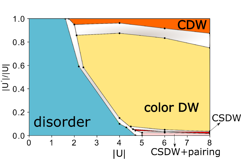
Figure 1: The low-temperature ($T=0.1$) phase diagram. The blue area is the disorder phase; the pink area is the phase where the CSDW order and the pairing order can be both detected; the red area is the CSDW phase; the yellow area is the color DW phase; the orange area is the CDW phase. The shaded areas represent the phase boundaries.

We then analyse how the anisotropy of interactions affects the symmetry of the Hamiltonian and affects the phase transitions. When $|U^{\prime}|/|U|=1$, the Hamiltonian has SU(3) symmetry. When $|U^{\prime}|/|U|\approx 1$, although the introduction of the anisotropy of interactions reduces the symmetry of the Hamiltonian from SU(3) to SU(2)$\otimes$ U(1), the system is still around the SU(3) symmetric points and it undergoes the disorder - CDW phase transition. When $\frac{5}{92}<|U^{\prime}|/|U|\leq\frac{7}{8}$, the anisotropy of interactions is obvious and the system is away from the SU(3) symmetric points. The system undergoes the disorder - color DW phase transition. When $\frac{1}{30}<|U^{\prime}|/|U|\leq\frac{5}{92}$, the mutual attraction $U_{13}$ and $U_{23}$ are so weak that fermions with spin component 3 decouple with fermions with other spin components. The system can enter into the CSDW phase in the large $|U|$ regime. When $|U^{\prime}|/|U|\leq\frac{1}{30}$, the system is around the SO(4)$\otimes$ U(1) symmetric point and it starts to show some features of the half-filled attractive SU(2) Hubbard model Lee et al. (2009): both the pairing order and the CSDW order can be detected in the large $|U|$ regime. When $|U^{\prime}|/|U|=0$, the system is divided into two subsystems: the two-component interacting fermions (with spin components 1 and 2) and free fermions (with spin component 3). The symmetry of the Hamiltonian is SO(4)$\otimes$ U(1) Yang and Zhang (1990); Xu (2011).

IV Cooper pair breaking

It is shown in the phase diagram Fig. 1 that the pairing order is quickly suppressed away from the SO(4)$\otimes$U(1) symmetric points. To explain this phenomenon, we need to rewrite the interaction term in Eq. (1) in the momentum spcae:

$$H_{\text{I}} =U\sum_{\vec{k}_{1}+\vec{k}_{2}=\vec{k}_{1}^{{}^{\prime}}+\vec{k}_{2}^{{}^{\prime}}}c_{1,\vec{k}_{1}^{{}^{\prime}}}^{\dagger}c_{2,\vec{k}_{2}^{{}^{\prime}}}^{\dagger}c_{2,\vec{k}_{2}}c_{1,\vec{k}_{1}}$$ (4)

$$+U^{\prime}\sum_{\vec{k}_{1},\vec{k}_{3},\Delta\vec{k}}c_{1,\vec{k}_{1}+\Delta\vec{k}}^{\dagger}c_{3,\vec{k}_{3}-\Delta\vec{k}}^{\dagger}c_{3,\vec{k}_{3}}c_{1,\vec{k}_{1}}$$

$$+U^{\prime}\sum_{\vec{k}_{2},\vec{k}_{3},\Delta\vec{k}}c_{2,\vec{k}_{2}+\Delta\vec{k}}^{\dagger}c_{3,\vec{k}_{3}-\Delta\vec{k}}^{\dagger}c_{3,\vec{k}_{3}}c_{2,\vec{k}_{2}},$$

in which $c_{\alpha,\vec{k}_{\alpha}}$ is the annihilation operator of the fermion with spin component $\alpha$ and momentum $\vec{k}_{\alpha}$. $H_{\text{I}}$ describes the on-site scatterings between fermions with different spin components. We then rewrite the pairing order parameter in the momentum space:

$$P=\frac{1}{N^{2}}\sum_{\vec{k}\vec{k^{\prime}}}\langle c_{1,\vec{k}^{\prime}}^{\dagger}c_{2,-\vec{k}^{\prime}}^{\dagger}c_{2,-\vec{k}}c_{1,\vec{k}}+h.c.\rangle.$$ (5)

Only Cooper pairs of spin components 1 and 2 contribute to $P$. The $U$ term in Eq.(4) scatters one Cooper pair ($2$,$-\vec{k}$;$1$,$\vec{k}$) into another Cooper pair ($2$,$-\vec{k^{\prime}}$;$1$,$\vec{k^{\prime}}$) so it does not reduce the number of Cooper pairs. However, the $U^{\prime}$ terms in Eq.(4) can destroy Cooper pairs, which is plotted in Fig. 2.

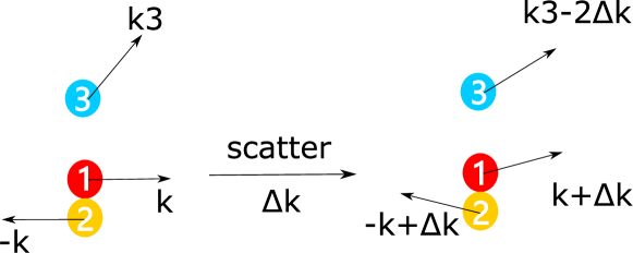
Figure 2: The on-site scattering process which destroys Cooper pairs.

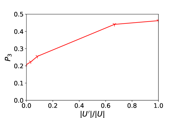
Figure 3: The on-site triple occupancy $P_{3}$ as a function of $|U^{\prime}|/|U|$ when $|U|=6$ and $T=0.1$. The lattice size is $L=9$.

When $|U|^{\prime}$ increases, the probability of on-site scattering process in Fig. 2 increases, since the on-site triple occupancy $P_{3}=\frac{1}{N}\sum_{i}\langle n_{i1}n_{i2}n_{i3}\rangle$ increases, as is shown in Fig.3. As a result, with increasing $|U^{\prime}|$, fewer Cooper pairs contribute to $P$ and the pairing order is suppressed.

V Néel ordering

In this section, we study the magnetic properties of our model. We choose to define the Néel order parameter along the same line as Ref. Zhou et al. (2014b). In our model, the Néel configuration can be chosen as follows: each site in sublattice A is filled with two fermions with spin components 1 and 2 while each site in sublattice B is filled with one fermion with spin component 3. The magnetic moment operator on site $i$ is defined as:

$$m_{i}=\frac{1}{4}(n_{i1}+n_{i2}-2n_{i3}).$$ (6)

For the configuration defined above, the value of the Néel moment is $m_{i}=(-1)^{i}\frac{1}{2}$. The Néel order parameter is defined as

$$m_{Q}=\frac{1}{N}\sqrt{\sum_{ij}(-1)^{i+j}m_{i}m_{j}},$$ (7)

in which $N$ represents the number of lattice sites.

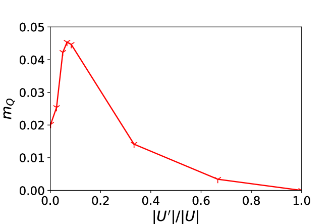
Figure 4: The Néel order parameter $m_{Q}$ versus $|U^{\prime}|/|U|$ at $T=0.1$ and $|U|=6$. The figure shows the results in the thermodynamic limit.

By doing finite-size extrapolations, we obtain the $m_{Q}$ versus $|U^{\prime}|/|U|$ relations in the thermodynamic limit at $T=0.1$ and $|U|=6$. The results are presented in Fig. 4. When the anisotropy of interaction is introduced (when $|U^{\prime}|/|U|<1$), the Néel order appears. The origin of the Néel order can be explained in a perturbative view. We first take the interaction term in Eq. (1) as $H_{0}$ and the hopping term in Eq. (1) as $H^{\prime}$. Then, we do the perturbation on a two-site toy model and get the first-order correction of the wave function:

$$|\psi_{\text{two-site}}\rangle=|123,0\rangle$$ (8)

$$+\frac{t}{2|U^{\prime}|}|12,3\rangle+\frac{t}{|U|+|U^{\prime}|}|13,2\rangle+\frac{t}{|U|+|U^{\prime}|}|23,1\rangle,$$

in which $|123,0\rangle$ represents an on-site trion while $|12,3\rangle$ ($|13,2\rangle$ and $|23,1\rangle$) represents an off-site trion with two fermions locating on site 1 and one fermion locating on site 2. When $|U^{\prime}|/|U|<1$, the density of off-site trions $|12,3\rangle$ is greater than the density of other two types of off-site trions. Hence, the SU(3) symmetry is broken. Subsequently, we put off-site trions into the lattice. When an off-site trion distributes as shown in Fig. 5(a), two hopping channels are blocked by Pauli exclusion; when an off-site trion distributes as shown in Fig. 5(b), four hopping channels are blocked by Pauli exclusion. To lower the total energy, off-site trions tend to distributes as shown in Fig. 5(a), which breaks the lattice inversion symmetry. Hence, when the anisotropy of interaction is introduced, off-site trions break both the SU(3) symmetry and the lattice inversion symmetry so Néel order appears.

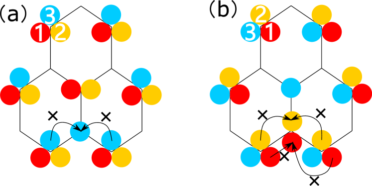
Figure 5: (a)Two hopping channels are blocked because of the distribution of the off-site trion. (b)Four hopping channels are blocked because of the distribution of the off-site trion.

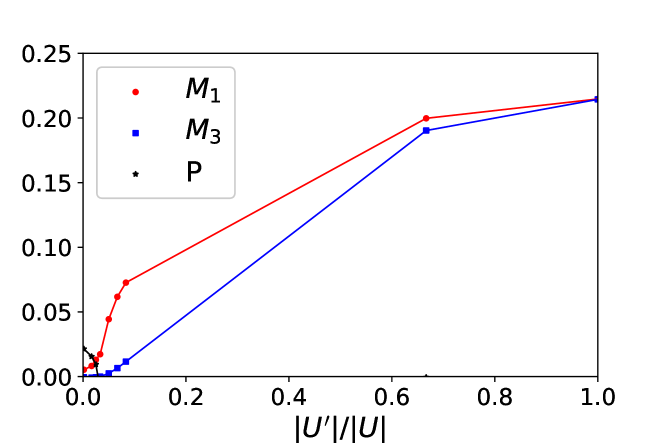
Figure 6: $M_{1}$, $M_{3}$ and $P$ as functions of $|U^{\prime}|/|U|$ when $T=0.1$ and $|U|=6$. The figure shows the results in the thermodynamic limit.

$m_{Q}$ is nonmonotonic with $|U^{\prime}|/|U|$. To exlpain this phenomenon, we calculate $M_{1}$, $M_{3}$ and $P$ as functions of $|U^{\prime}|/|U|$, which are presented in Fig. 6. Actually, the strength of $m_{Q}$ is determined by the density difference $\Delta n=|n_{i1}+n_{i2}-2n_{i3}|$ on each site. Around the SU(3) symmetric points, $M_{1}\approx M_{3}$. Fermions with different spin components tend to bind together so $\Delta n$ is very small. Around the SO(4)$\otimes$U(1) symmetric points (characterized by $M_{3}=0$ and $P>0$), fermions with spin component 3 are itinerant ($M_{3}=0$) and the CDW order of spin component 1 and 2 is weak ($M_{1}\rightarrow 0$). Hence, $\Delta n$ is small in this case. Away from the SU(3) symmetric points and the SO(4)$\otimes$U(1) symmetric points, a considerable number of off-site trions $|12,3\rangle$ exist, which contributes to $\Delta n$. Hence, the peak of $m_{Q}$ develops away from the SU(3) symmetric points and the SO(4)$\otimes$U(1) symmetric points.

VI thermodynamic properties

In this section, we present the thermodynamic properties of our model, including the entropy-temperature relations and the density compressibility-temperature relations.

VI.1 the entropy-temperature relations

In our simulations, the entropy per particle is calculated through:

$$\frac{S(T)}{k_{\text{B}}}=\frac{S(\infty)}{k_{\text{B}}}+\beta E(\beta)-\int_{0}^{\frac{1}{T}}d\beta E(\beta),$$ (9)

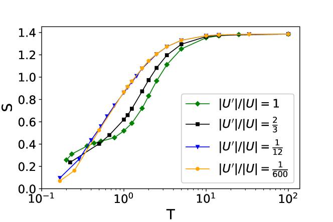
Figure 7: The entropy per particle $S$ versus $T$ at different values of $|U^{\prime}|/|U|$ when $|U|=6$. The lattice size is $L=9$.

in which $E(\beta)$ is the internal energy per particle at inverse temperature $\beta=\frac{1}{T}$ Li et al. (2021). In Fig. 7, we present the entropy per particle $S$ as a function of $T$ at different values of $|U|^{\prime}/|U|$ when $|U|=6$. At low temperatures, the system is in the CDW state when $\frac{|U^{\prime}|}{|U|}=1$. Its entropy is mainly contributed by the charge fluctuations of on-site trions, as is shown in Fig. 8 (a). When $\frac{|U^{\prime}|}{|U|}$ is obviously smaller than 1, the system is in the color DW state. The charge fluctuations of on-site trions are suppressed because off-site trions $|12,3\rangle$ form Néel order, as is shown in Fig. 8 (b). When $\frac{|U^{\prime}|}{|U|}\approx 0$, pairing order appears. The entropy of the system is mainly contributed by fermions (with spin component 3) near the Dirac points and Cooper pairs (of spin components 1 and 2) near the fermi surface. Hence, when $|U^{\prime}|/|U|$ decreases from 1 to 0, the system becomes more ordered at the same temperature in the low temperature regime. Because of this, our system can be driven to lower temperatures adiabatically by increasing $|U^{\prime}|/|U|$ from $\frac{1}{600}$ to $1$. This anisotropy of interactions induced adiabatic cooling may provide a new method to cool a system in experiments.

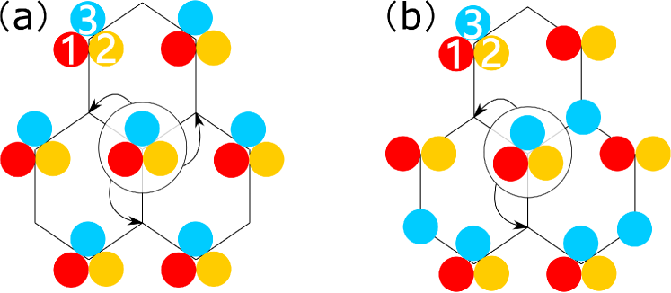
Figure 8: (a) The charge fluctuations of on-site trions in the CDW state. There exist three hopping channels for the central on-site trion. (b) The charge fluctuations of on-site trions in the color DW state. Because off-site trions $|12,3\rangle$ form Néel order on the lattice, one hopping channel for the central on-site trion is blocked. The charge fluctuations of on-site trions are suppressed in the color DW state.

VI.2 the density compressibility-temperature relations

The density compressibility is defined as

$$\kappa=\frac{\beta}{2L^{2}}\left(\left<\left(\sum_{i}n_{i}\right)^{2}\right>-\left<\sum_{i}n_{i}\right>^{2}\right),$$ (10)

which reflects the global density fluctuaions.

we present our DQMC simulation results for the density compressibility in Fig. 9. When $T\rightarrow 0.1$, $\kappa$ is nearly suppressed to zero if $|U^{\prime}|/|U|\geq\frac{1}{12}$, which is a signature of the Mott insulating states Schneider et al. (2008); Duarte et al. (2015). In this situation, the system is either in the color DW state or the CDW state. However, when $|U^{\prime}|/|U|=\frac{1}{600}$, $\kappa\gg 0$. In this situation, fermions with spin component 3 are itinerant while fermions with spin components 1 and 2 form Cooper pairs. The system is not a Mott insulator.

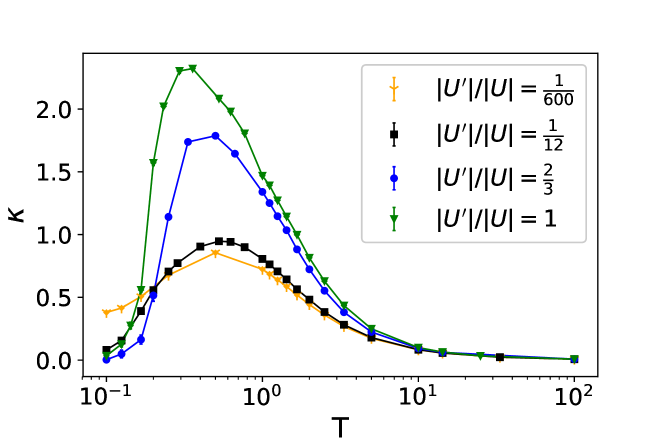
Figure 9: The density compressibility $\kappa$ versus $T$ at different values of $|U^{\prime}|/|U|$ when $|U|=6$. The lattice size is $L=9$.

VII Conclusions and discussions

We have employed the DQMC simulations to study the thermodynamic properties of the half-filled attractive three-component Hubbard model on a honeycomb lattice. We calculate the low-temperature phase diagram, the magnetic properties, the entropy-temperature relations and the density compressibility.

The anisotropy of interactions affects the symmetry of the Hamiltonian and affects the phase transitions. When $|U^{\prime}|/|U|$ decreases from $1$ to $0$, the symmetry of the Hamiltonian changes from SU(3) to SU(2)$\otimes$ U(1) and finally to SO(4)$\otimes$ U(1). Around the SU(3) symmetric points, the system undergoes the disorder - CDW phase transition. Away from the SU(3) and the SO(4)$\otimes$ U(1) symmetric points, the system can enter into the color DW phase or the CSDW phase. Around the SO(4)$\otimes$ U(1) symmetric points, both the pairing order and the CSDW order can be detected. Away from the SO(4)$\otimes$ U(1) symmetric points, the pairing order is quickly suppressed because the $|U^{\prime}|$ terms introduce the scattering process which destroys Cooper pairs. When anisotropy of interactions is introduced, the Néel order appears because the number of off-site trions $|12,3\rangle$ is greater than the number of other two types of off-site trions and off-site trions $|12,3\rangle$ do not distribute randomly. Finally, we calculate the entropy-temperature relations and find the anisotropy of interactions induced adiabatic cooling. This may provide a new method to cool a system in experiments.

Appendix A The Hubbard-Stratonovich Decomposition for three-component Hubbard interaction

The partition function of our model is

$$Z=\mbox{tr}\left\{H\right\}=\mbox{tr}\left\{\prod_{k=1}^{M}e^{-\Delta_{\tau}H_{k}}e^{-\Delta_{\tau}H_{U}}\right\}+{\cal O}(\Delta_{\tau}^{2}),$$ (11)

in which we apply the Trotter-Suzuki decomposition to seperate the kinetic term and the interaction term. $\Delta_{\tau}=\frac{\beta}{M}$ is the discrete imaginary-time interval. The explicit form of the interaction term is

$$e^{-\Delta_{\tau}\sum_{i,\alpha<\beta}U_{\alpha\beta}(n_{i\alpha}-\frac{1}{2})(n_{i\beta}-\frac{1}{2})}$$ (12)

$$=\prod_{i,\alpha<\beta}e^{-\frac{\Delta_{\tau}U_{\alpha\beta}}{2}(c_{i\alpha}^{\dagger}c_{i\beta}-h.c.)^{2}-\frac{\Delta_{\tau}U_{\alpha\beta}}{4}}.$$

The interaction term can be diagonalized in the new basis of complex fermion operators,

$$\tilde{c}_{\alpha\beta}=\frac{1}{\sqrt{2}}(c_{\alpha}-ic_{\beta}),\tilde{c}_{\beta\alpha}=\frac{1}{\sqrt{2}}(c_{\alpha}+ic_{\beta}).$$ (13)

The complex fermion operators $\tilde{c}_{\alpha\beta}$, $\tilde{c}_{\beta\alpha}$ obey fermionic anticommutation relations : $\{\tilde{c}_{\alpha\beta}^{\dagger},\tilde{c}_{\alpha\beta}\}=1$, $\{\tilde{c}_{\alpha\beta}^{\dagger},\tilde{c}_{\beta\alpha}\}=0$ and $\{\tilde{c}_{\beta\alpha}^{\dagger},\tilde{c}_{\beta\alpha}\}=1$. In the new basis, $(c_{i\alpha}^{\dagger}c_{i\beta}-h.c.)^{2}=-(\tilde{c}_{\alpha\beta}^{\dagger}\tilde{c}_{\alpha\beta}-\tilde{c}_{\beta\alpha}^{\dagger}\tilde{c}_{\beta\alpha})^{2}$. For simplicity, we construct the Hubbard-Stratonovich (H-S) decomposition in the new basis on one site,

$$\prod_{\alpha<\beta}e^{\frac{\Delta_{\tau}U_{\alpha\beta}}{2}(\tilde{c}_{\alpha\beta}^{\dagger}\tilde{c}_{\alpha\beta}-\tilde{c}_{\beta\alpha}^{\dagger}\tilde{c}_{\beta\alpha})^{2}}$$ (14)

$$=\prod_{\alpha<\beta}\frac{1}{2}\sum_{s_{\alpha\beta}=\pm 1}e^{is_{\alpha\beta}\lambda_{\alpha\beta}(\tilde{c}_{\alpha\beta}^{\dagger}\tilde{c}_{\alpha\beta}-\tilde{c}_{\beta\alpha}^{\dagger}\tilde{c}_{\beta\alpha})},$$

in which $\lambda_{\alpha\beta}=\arccos e^{\frac{\Delta_{\tau}U_{\alpha\beta}}{2}}$. Returning to the original basis, the H-S decomposition of the interaction term on one site is:

$$e^{-\Delta_{\tau}\sum_{\alpha<\beta}U_{\alpha\beta}(n_{\alpha}-\frac{1}{2})(n_{\beta}-\frac{1}{2})}$$ (15)

$$=\frac{1}{8}e^{-\frac{\Delta_{\tau}}{4}(U_{12}+U_{13}+U_{23})}\prod_{\alpha<\beta}\sum_{s_{\alpha\beta}=\pm 1}e^{s_{\alpha\beta}\lambda_{\alpha\beta}(c^{\dagger}_{\alpha}c_{\beta}-c_{\beta}^{\dagger}c_{\alpha})}.$$

References

- Taie et al. (2010) S. Taie, Y. Takasu, S. Sugawa, R. Yamazaki, T. Tsujimoto, R. Murakami, and Y. Takahashi, Phys. Rev. Lett. 105, 190401 (2010).
- DeSalvo et al. (2010) B. J. DeSalvo, M. Yan, P. G. Mickelson, Y. N. Martinez de Escobar, and T. C. Killian, Phys. Rev. Lett. 105, 030402 (2010).
- Taie et al. (2012) S. Taie, R. Yamazaki, S. Sugawa, and Y. Takahashi, Nat. Phys. 8, 825 (2012).
- Scazza et al. (2014) F. Scazza, C. Hofrichter, M. Höfer, P. D. Groot, I. Bloch, and S. Fölling, Nat. Phys. 10, 779 (2014).
- Zhang et al. (2014) X. Zhang, M. Bishof, S. L. Bromley, C. V. Kraus, M. S. Safronova, P. Zoller, A. M. Rey, and J. Ye, Science 345, 1467 (2014).
- Pagano and et al. (2014) G. Pagano and et al., Nat. Phys. 10, 198 (2014).
- Cazalilla and Rey (2014) M. A. Cazalilla and A. Rey, Rep. Prog. Phys. 77, 124401 (2014).
- Hofrichter et al. (2016) C. Hofrichter, L. Riegger, F. Scazza, M. Höfer, D. R. Fernandes, I. Bloch, and S. Fölling, Phys. Rev. X 6, 021030 (2016).
- Huckans et al. (2009) J. H. Huckans, J. R. Williams, E. L. Hazlett, R. W. Stites, and K. M. O’Hara, Phys. Rev. Lett. 102, 165302 (2009).
- Courteille et al. (1998) P. Courteille, R. S. Freeland, D. J. Heinzen, F. A. van Abeelen, and B. J. Verhaar, Phys. Rev. Lett. 81, 69 (1998).
- Inouye et al. (1998) S. Inouye, M. Andrews, J. Stenger, H.-J. Miesner, D. Stamper-Kurn, and W. Ketterle, Nature 392, 151 (1998).
- Bloch et al. (2008) I. Bloch, J. Dalibard, and W. Zwerger, Rev. Mod. Phys. 80, 885 (2008).
- Wang et al. (2014) D. Wang, Y. Li, Z. Cai, Z. Zhou, Y. Wang, and C. Wu, Phys. Rev. Lett. 112, 156403 (2014).
- Zhou et al. (2014a) Z. Zhou, Z. Cai, C. Wu, and Y. Wang, Phys. Rev. B 90, 235139 (2014a).
- Zhou et al. (2016) Z. Zhou, D. Wang, Z. Y. Meng, Y. Wang, and C. Wu, Phys. Rev. B 93, 245157 (2016).
- Zhou et al. (2017) Z. Zhou, D. Wang, C. Wu, and Y. Wang, Phys. Rev. B 95, 085128 (2017).
- Zhou et al. (2018) Z. Zhou, C. Wu, and Y. Wang, Phys. Rev. B 97, 195122 (2018).
- Rapp and Rosch (2011) A. Rapp and A. Rosch, Phys. Rev. A 83, 053605 (2011).
- Nie et al. (2017) W. Nie, D. Zhang, and W. Zhang, Phys. Rev. A 96, 053616 (2017).
- Xu et al. (2019) H. Xu, Z. Zhou, X. Wang, L. Wang, and Y. Wang, “Quantum monte carlo simulations of the attractive su(3) hubbard model on a honeycomb lattice,” (2019), arXiv:1912.11233 [cond-mat.quant-gas] .
- Li et al. (2021) X. Li, H. Xu, and Y. Wang, “Thermal charge-density-wave transition and trion formation in the attractive su(3) hubbard model on a honeycomb lattice,” (2021), arXiv:2101.00804 [cond-mat.quant-gas] .
- Inaba et al. (2010) K. Inaba, S.-y. Miyatake, and S.-i. Suga, Phys. Rev. A 82, 051602 (2010).
- Yanatori and Koga (2016) H. Yanatori and A. Koga, Journal of the Physical Society of Japan 85, 014002 (2016).
- Hasunuma et al. (2016) T. Hasunuma, T. Kaneko, S. Miyakoshi, and Y. Ohta, Journal of the Physical Society of Japan 85, 074704 (2016).
- Inaba and Suga (2009) K. Inaba and S.-i. Suga, Phys. Rev. A 80, 041602 (2009).
- Miyatake et al. (2011) S.-y. Miyatake, K. Inaba, and S.-i. Suga, Journal of Physics: Conference Series 273, 012008 (2011).
- Okanami et al. (2014) Y. Okanami, N. Takemori, and A. Koga, Phys. Rev. A 89, 053622 (2014).
- Blankenbecler et al. (1981) R. Blankenbecler, D. J. Scalapino, and R. L. Sugar, Phys. Rev. D 24, 2278 (1981).
- Hirsch (1985) J. E. Hirsch, Phys. Rev. B 31, 4403 (1985).
- Wang et al. (2015) L. Wang, Y.-H. Liu, M. Iazzi, M. Troyer, and G. Harcos, Phys. Rev. Lett. 115, 250601 (2015).
- Lee et al. (2009) K. L. Lee, K. Bouadim, G. G. Batrouni, F. Hébert, R. T. Scalettar, C. Miniatura, and B. Grémaud, Phys. Rev. B 80, 245118 (2009).
- Yang and Zhang (1990) C. N. Yang and S. Zhang, Mod. Phys. Lett. B 04, 759 (1990).
- Xu (2011) C. Xu, Phys. Rev. B 83, 024408 (2011).
- Zhou et al. (2014b) Z. Zhou, Z. Cai, C. Wu, and Y. Wang, Phys. Rev. B 90, 235139 (2014b).
- Schneider et al. (2008) U. Schneider, L. Hackermüller, S. Will, T. Best, I. Bloch, T. A. Costi, R. W. Helmes, D. Rasch, and A. Rosch, Science 322, 1520 (2008).
- Duarte et al. (2015) P. M. Duarte, R. A. Hart, T.-L. Yang, X. Liu, T. Paiva, E. Khatami, R. T. Scalettar, N. Trivedi, and R. G. Hulet, Phys. Rev. Lett. 114, 070403 (2015).