Swapping Semantic Contents for Mixing Images
Abstract
Deep architecture have proven capable of solving many tasks provided a sufficient amount of labeled data. In fact, the amount of available labeled data has become the principal bottleneck in low label settings such as Semi-Supervised Learning. Mixing Data Augmentations do not typically yield new labeled samples, as indiscriminately mixing contents creates between-class samples. In this work, we introduce the SciMix framework that can learn to replace the global semantic content from one sample. By teaching a StyleGan generator to embed a semantic style code into image backgrounds, we obtain new mixing scheme for data augmentation. We then demonstrate that SciMix yields novel mixed samples that inherit many characteristics from their non-semantic parents. Afterwards, we verify those samples can be used to improve the performance semi-supervised frameworks like Mean Teacher or Fixmatch, and even fully supervised learning on a small labeled dataset.
I Introduction
Deep architectures have proven capable of reliably solving a variety of tasks such as classification [1, 2], object detection [3] or machine translation [4]. This is however contingent on there being a large amount of labeled data to train models on. This is seldom the case in practical applications where labelisation tends to be costly.
Data Augmentation [5, 6] - the creation of artificial samples from existing ones - has long been used to help models train on small datasets. Of particular interest in low label settings like Semi-Supervised Learning [7, 8] (SSL), Mixing Samples Data Augmentations [9, 10] (MSDA) can be used to combine the few samples that are either labeled or reliably pseudo-labeled with the large pool of unlabeled data. Unfortunately, Mixing Data Augmentations mix contents indiscriminately and as such create between-class hybrids for classification. While such hybrids have proven very useful for model regularization [11, 12], this process strongly perturbs the semantic information from reliably labeled samples.
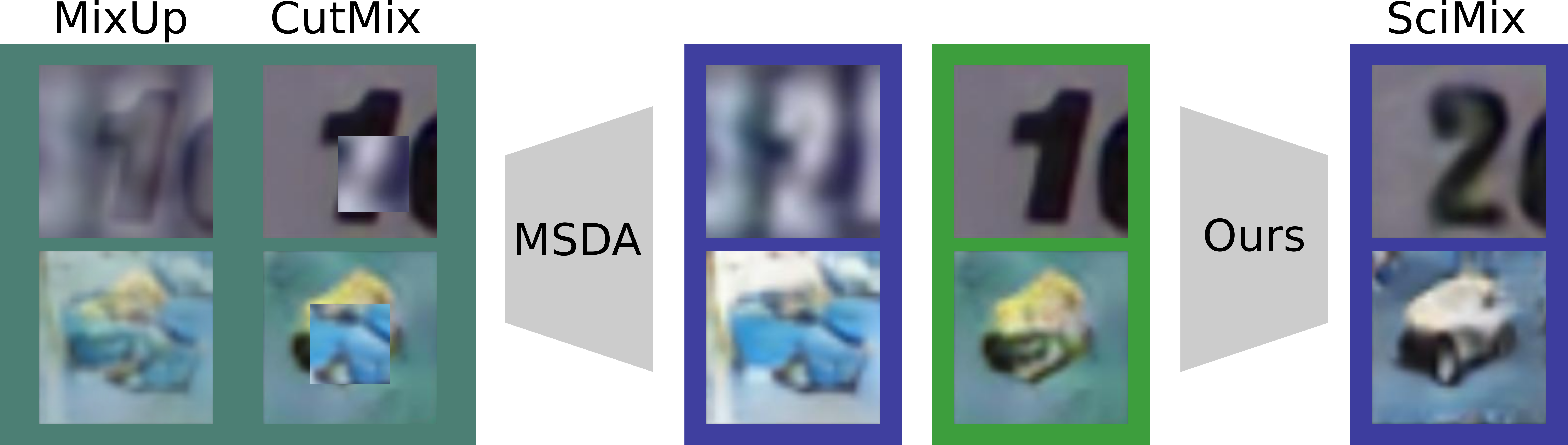
We argue that, with the right adjustments, mixing data augmentations can still be used to teach semantic invariance to neural networks. Indeed, if we can mix the semantic content of one sample with the non-semantic content of another, then the generated samples will still be actual in-class samples. For instance, Fig. 1 shows that mixing two street numbers with MixUp or CutMix typically leads to no real number appearing on the image whereas carefully selecting the contents to be mixed leads to a mixed sample that remains realistic.
In this paper, we introduce SciMix a new framework that learns to separate semantic from non semantic content and generate hybrids that preserve most of the specified non semantic content while still properly representing the required semantic content. Moreover, we demonstrate hybrids generated from this framework improve model performance through extensive low label experiments, primarily on the Semi-Supervised Learning problem (CIFAR10 and SVHN). We therefore propose three main contributions: 1) A new mixing paradigm designed to create artificial in-distribution samples that embed the non-semantic content of one sample into the non-semantic context of another. This new approach generates a new type of data augmentation for deep learning. 2) A new auto-encoding architecture and associated learning scheme that trains a generator to mix semantic and non-semantic contents. In particular, we purposefully train a model to separate semantic and non-semantic contents into two representations, and train a style-inspired generator to embed the semantic content (“style” code) into the non-semantic background (traditional input). 3) A new learning process to leverage our new mixing data augmentation. We show mixed samples can be used to optimize an additional supervised objective that significantly improves classifier performance.
II SciMix Framework
We propose in this paper a new mixing data augmentation that mixes the semantic content of a sample with the non-semantic content of another. As such, we first detail our scheme to train a model capable of mixing samples as per our exact specifications (Sec. II-A). We then explain our data augmentation strategy for visual classification leveraging our generated semantic hybrid samples (Sec. II-B). Finally, we discuss SciMix in the broader context of content mixing techniques (Sec. II-C).
II-A Learning to generate hybrids
Auto-encoding architecture
Our framework is based on a novel auto-encoder architecture presented in Fig. 2a that treats semantic information as a global characteristic of an encoded image. An input is projected into a semantic latent space by an encoder as well as a complementary non-semantic latent space by an encoder . While our framework should primarily be understood as an auto-encoder framework, the distinct nature of the latent spaces and requires more careful consideration. We choose in this paper to focus on the definition and exploitation of the semantic features , and simply treat as information irrelevant to . In other words, we design the framework so that the semantic information controls what the generator reconstructs. As the notion of semantic information is fundamentally tied to that of the tasks under consideration, we define with respects to a classifier. More precisely, we treat the semantic latent space as the feature space of a classifier. To this end, we add a linear neural layer on top of (see Fig. 2a) that outputs a class prediction . Note that therefore constitutes a standard CNN classifier [1, 13]. We ensure the classifier correctly learns semantic information through classification loss term on its output 111 can correspond to any classifier training framework (e.g. supervised training, FixMatch [14]). In semi-supervised experiments, we use Mean Teacher [15] as a simple classifier guide in order to leverage SSL datasets..
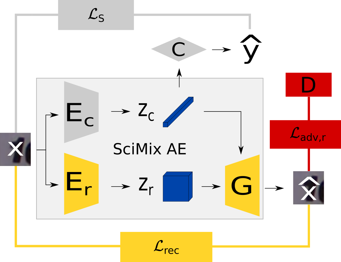
Contrarily to [16], we complete the encoding with a generator G that computes a reconstruction using the non-semantic features as direct inputs and the semantic features as style codes. This makes the non-semantic content easier to transfer, which is fortunate considering we can ensure semantic transfer more easily through a classifier (see Sec. III-E for the converse approach). As we treat the model as an autoencoder, we use a reconstruction loss to tie the reconstruction to the input . We further refine this reconstruction by using an adversarial critic to smooth out details [16]. We add a discriminator network (see Fig. 2a) to predict whether the considered image is a real sample or a reconstruction . Conversely, , and are trained to fool into seeing reconstructions as real images. The resulting loss serves to improve reconstructions learned through the reconstruction loss.
| (1) |
Finally, our learning scheme is based on the minimization of the loss composed of and , plus an additional loss term:
| (2) |
which is described in the following hybridizing scheme.
Hybridization losses
Simply training the auto-encoder architecture, even with as the feature space of a classifier, is not enough to ensure that hybrids correctly inherit characteristics from their parents. To force the model to properly inject semantic content into the general background of known samples, we design explicit hybridization losses (studied more closely in Sec. III-E)
| (3) |
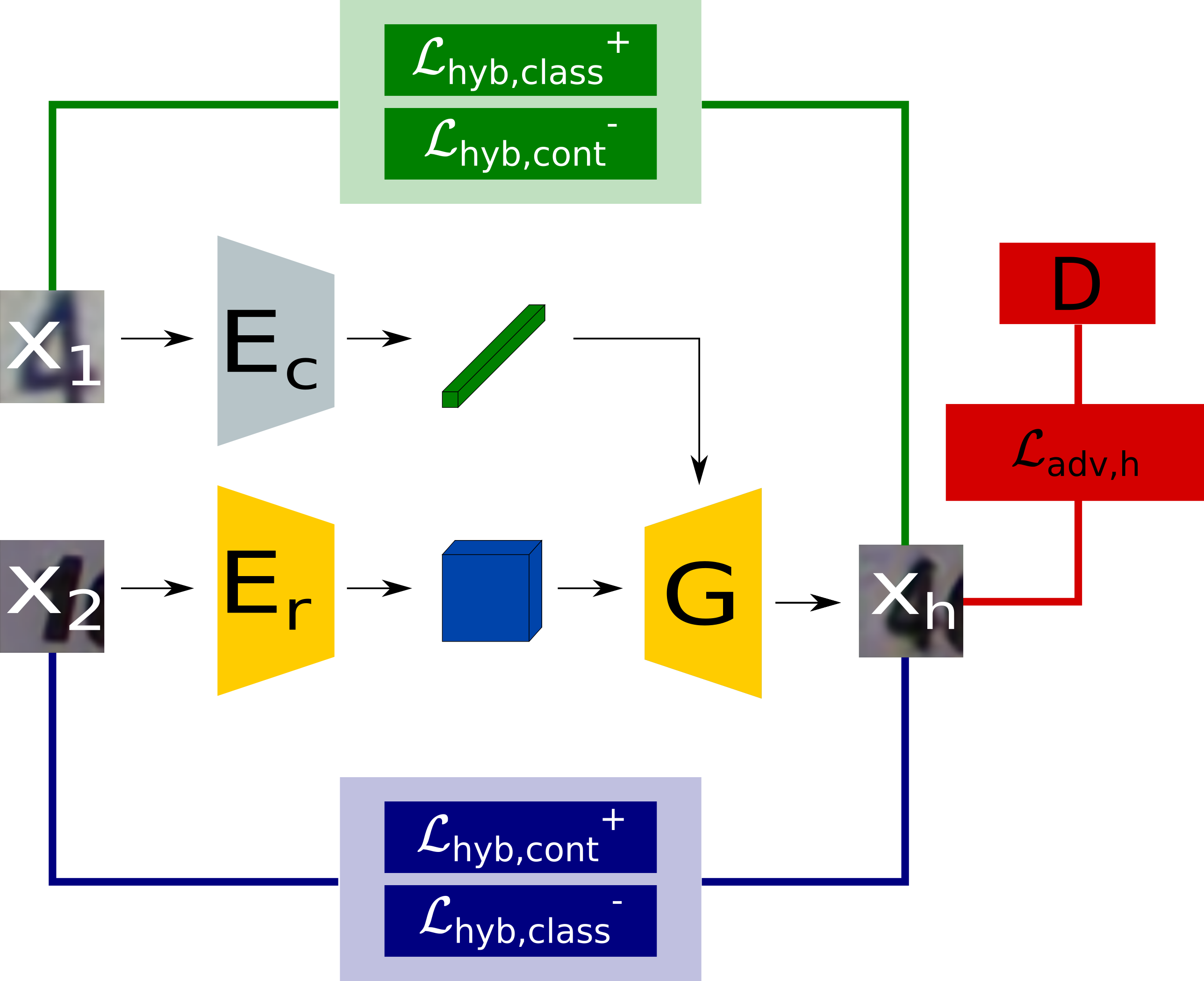
explicitly trains our model to rely on to generate the main semantic object in the generated reconstruction/hybrid. Indeed, we rely on the classifier ’s ability to identify and classify the main object in inputs (see Fig. 2b).
Put plainly, we generate hybrids from pairs of samples in a batch and obtain logits predictions for those hybrids. optimizes the model so that this prediction on the logits match the prediction on the semantic parent of . Importantly, we only optimize the hybridization process that generates : we do not optimize the classifier’s prediction on or . The idea is that the autoencoder learns to place in the right class manifold, while said class manifold does not move to accommodate :
| (4) |
Similarly, optimizes the model so that a generated hybrids ’s non-semantic representation matches its non semantic parent ’s non semantic component . As in the semantic case, we only optimize the generative process that leads to the generation of but do not optimize to project close to its non-semantic parent:
| (5) |
We also train hybrids to differ from their parents through the negative semantic hybridization loss and the negative non-semantic hybridization loss . In practice, this means maximizing the distance between hybrids and semantic (resp. non-semantic) parent in non-semantic (resp. semantic) space.
To ensure the quality of generated hybrids, we train the discriminator to also recognize hybrids as synthetic images. With this discriminator we can simply add an adversarial loss term to ensure hybrids look realistic (as far as is concerned).
II-B Training a classifier by leveraging our Data Augmentation
We now have a novel mixing data augmentation that can embed the semantic content of one sample to the non-semantic context of other samples, given a trained generator. This provides a useful and new way to improve any standard training method “X” by adding a single additional loss term : .
Generating hybrids given a trained autoencoder
Generating hybrids given a trained model is straightforward (Fig. 2b shows how a hybrid is mixed). Specifically, given samples (with known label ) and , we extract the relevant features , , and . is now a sample with class . As a conservative measure, we only keep the generated hybrid if to avoid disturbing decision boundaries too much. Note that with this, we generate a strong augmentation of and teach the classifier to group with its strongly augmented version in a similar line to work in contrastive representation learning [17].
Training a new classifier
We now propose a way to leverage our novel hybrids to improve the training of standard models such as Mean Teacher [15] or FixMatch [14]. To this end, we compute hybrids that mix the semantic content of each sample in the batch with the non-semantic content of other samples in the batch. We leverage those hybrids by optimizing an additional loss:
| (6) |
This new loss takes advantage of our mixing paradigm by mostly imputing the semantic parent’s label to our hybrids, with only a slight dependence on the non-semantic parent to acknowledge the imperfection of the mixing process. Contrarily to standard mixing augmentations, the ratio is a fixed hyperparameter (in the spirit of label smoothing [18]).
II-C Mixing contents in the literature
Mixing of one type of content with another is more readily found in unsupervised image-to-image translation: models are trained to translate the content of one image to the “domain” of another, though these terms are rarely well defined. Interestingly, bi-modal auto-encoding architectures appear fairly early on in this literature [19, 20]. Incidentally, more recent works in few-shot translation [21] and unsupervised translation [22] have even started associating the domain (or class) information to a style code fed as input to a StyleGan inspired decoder. In a more supervised fashion, such methods have been used to combine textures (domain information) with structural information (image information) [16]. This line of work however is specifically tailored to image generation and fails to leverage information to from fully fledged classifier to learn complex semantic variations.
Style transfer actually tackles the issue of mixing different types of contents in a similar fashion to our framework. The main difference between such frameworks and our problem lies in the definition of the contents to mix. In style transfer, the distinction is made between a style code and a structure code while we seek to mix semantic and non-semantic content. As such, our work reprises feature map modulation mechanisms that have been proven to work in style transfer [23, 24, 25] but makes use of additional losses to ensure we mix semantic and non-semantic contents.
It is worth noting that our goal of generating images in a way such that semantic content can be modified independently of non semantic content echoes that of disentangled generation [26, 27, 28, 29]. Importantly however, we aim to modify only a single coarse attribute rather than separate a multitude of fine grained characteristics.
III Experiments
We demonstrate here how our SciMix data augmentation can be leveraged to improve training in low-label settings. To this end, we conduct extensive experiments on the semi-supervised problem on the CIFAR10 [30] and SVHN [31] datasets. Additionally, we propose in Sec. III-G a study of SciMix’s performance in a fully supervised setting with few labels on a variation of the CUB-200 [32] dataset.
In the semi-supervised case, we show SciMix improves two backbone methods: Mean Teacher [15] and FixMatch [8] (refer to Sec. II-B for how we apply our framework to these methods). We chose Mean Teacher as a reference consistency-based baseline. Beyond its widespread use in SSL, consistency induces a stabilization we feel would help extract invariant semantic features. FixMatch is a state-of the art SSL method based on strong augmentation, and often serves as a reference or backbone in the literature [33, 34].
We operate on a standard WideResNet-28-2 [13] for our classifiers (both and ). follows the same architecture as . The skeleton of follows a StyleGanv2 [35] architecture. Hyperparameters and optimizers were generally taken to follow settings reported in the base methods’ original papers [15, 8].
We report the classification accuracy over 3 seeded runs for varying numbers of labeled samples in a dataset (the rest are treated as unlabeled). The SciMix generators used to train a model with labeled samples are also trained with only labeled samples. One generator is trained per setting, and classifiers trained with the generator’s mixed samples are trained on the same split of labeled/unlabeled data to avoid information leakage. More details for all experiments are given in Appendix.
III-A Performance gains
Tab. I shows that adding our optimization on hybrids with - as described in Sec. II-B - does indeed lead to improved performance on CIFAR10 and SVHN. Indeed, training with SciMix hybrids leads to significant accuracy gains with a Mean Teacher classifier with a wide range of labeled samples. We also observe improvements over FixMatch on very low labeled settings (FixMatch performance quickly saturates on higher labeled settings). Interestingly, two concurrent behaviors can be observed on Mean Teacher: SciMix hybrids become more useful when less labeled samples are available but the quality of generated hybrids becomes unreliable with few labeled samples. Indeed, at 100 labeled samples on CIFAR10, the Mean Teacher classifier used to train the generator is too weak to provide very useful hybrids. With a strong SciMix hybridizer (trained with all samples), SciMix data augmentation would bring a Mean Teacher classifier to an accuracy of with 100 labels on CIFAR10.
III-B Quality of hybridization
We now verify the auto-encoder described in Sec. II-A indeed yields interesting hybrids for data augmentation. This can be observed qualitatively by considering the generated hybrids (see Fig. 3a) and quantitatively in Tab. 3b through an observation of the generated hybrids in relation to their parents.


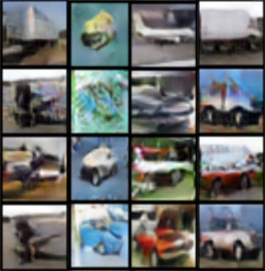
Fig. 3a shows hybrids generated by the method. As can be observed, SciMix creates hybrids that match the semantic content of the semantic parent while closely matching the non-semantic parents in every other regard. Qualitative samples suggest the framework properly identifies semantic content in the parent samples and successfully embeds the semantic content of the semantic parent into the non-semantic background of the non-semantic parent.
Preservation of semantic and non-semantic characteristics
We quantify how well the generated hybrids inherit properties from the semantic and non-semantic parents and through the metrics and . The semantic transfer rate is the accuracy of an “oracle” classifier (trained on the entire dataset, as a proxy for human evaluation of hybrid labels) over a dataset built from hybrids that are assumed to have inherited the label of their semantic parent. Conversely, the non-semantic preservation rate is the proportion of hybrids that are closer to the non-semantic parent in pixel space (ie, ).
Tab. 3b shows SciMix compares favorably to texture altering hybrids (FDA, AdaIN) and standard mixing augmentations (MixUp with the label of the dominant samples as suggested in [37]) on a strong generator (SVHN 250 labels). While most existing hybridizations do tend to preserve the semantic content, SciMix shines in that it transfers semantic content while keeping hybrids very close to their non-semantic parent. Indeed, other hybrids remain much closer to their semantic parent (always the case - by design - for MixUp).
III-C Comparison to Mixing Data Augmentation
We now show that in very low label settings, the “artificial” labelized samples SciMix can outperform the regularization offered by more traditional mixing Data Augmentation. Tab. II shows that SciMix mostly outperforms MixUp and CutMix for CIFAR10 with 250 labeled samples (the generator is too weak with 100 labels) and SVHN with 60 labeled samples (hardest setting). While MixUp does perform similarly to SciMix on CIFAR10, this is likely due to the low performance of the classifier trained with only 250 labels.
III-D Ablation: Regularization vs. Data Augmentation
While we evaluate our framework as a general data augmentation framework by using mixed samples from a pre-trained generator to train a model from scratch, it is interesting to note that our mixing auto-encoder also trains and uses a classifier model. We study in Tab. III the relative performance of the generator classifier (tied to the auto-encoder and regularized by but without mixed data augmentation) and of a classifier trained from scratch with our mixed data augmentation (but without explicit loss regularization). While the generator classifier does outperform the backbone classifier in all cases (showcasing the usefulness of the regularization scheme), training from scratch with data augmentation leads to better results on every setting. Interestingly, keeping the weights of the auto-encoder classifier as initialization to train a model with SciMix mixing does not necessarily outperform a random initialization. This can be explained by the fact that the separation characterized by the data augmentation is already learned by the auto-encoder classifier and therefore training with our hybrids fails to teach the model anything interesting.
III-E Model analysis: Importance of the learning scheme
Hybrids parent pairs
![[Uncaptioned image]](/html/2205.10158/assets/sample_hybrids_parents.png) Method
Accuracy
sample hybrids
Structural
Method
Accuracy
sample hybrids
Structural
![[Uncaptioned image]](/html/2205.10158/assets/sample_hybrids_structzc.png) No
No
![[Uncaptioned image]](/html/2205.10158/assets/sample_hybrids_no.png) Basic
Basic
![[Uncaptioned image]](/html/2205.10158/assets/sample_hybrids_pos.png) Non Frozen criterion
Non Frozen criterion
![[Uncaptioned image]](/html/2205.10158/assets/sample_hybrids_hybfull.png) Full Setup
Full Setup
![[Uncaptioned image]](/html/2205.10158/assets/sample_hybrids.png)
To better explore how our framework facilitates the incrustation of semantic content in the general context of existing samples, we first propose a rapid ablation study on the quality of the samples generated by variants of our auto-encoder on our hardest SVHN setting (60 labels). We evaluate this through the classification accuracy of models trained with the generator’s mixed samples, the semantic transfer , the non-semantic transfer , and a visual evaluation of two hybrids (e.g. the leftmost hybrid mixes a blue 8 with a yellow 3 ).
We consider 4 variations on SciMix’s generator to demonstrate the merits of our chosen method: as a style code. We flip the roles of and , to demonstrate is better used as a style code in SciMix. No . We train without an explicit optimization loss, to show and are not sufficient to create good hybrids in SciMix. Basic . We demonstrate the orthogonalization losses and contribute to the generator by considering a variant that does not optimize them. No frozen criterion . We do not force the generator to only optimize the generation of the hybrids when optimizing (the projection of the hybrids in the latent spaces is also modified).
Tab. IV shows that without explicit hybridization optimization, the model fails to properly transfer semantic characteristics (low score). Since the model does properly transfer semantic content with only , the addition of the orthogonalization constraints is not necessary to obtain useful hybrids. However, this orthogonalization increases the diversity in the generated hybrids and therefore leads to a better augmentation procedure. Not freezing the projection heads when training for hybridization on the other hand leads to a general deterioration of the training process and can therefore be felt in both transfer rates. Predictably, using as a global style code leads a very poor correspondence of hybrids to their non-semantic parents as things like backgrounds can become very complicated to reproduce with a modulation based generator.
III-F Model analysis: Leveraging the hybrids as Data Augmentation
| Method | Accuracy |
|---|---|
| Baseline | |
We considered 4 alternative methods to exploit the hybrids generated by our method: Labeled Only hybrids with a labeled semantic parent are considered (supervised training with a hard label) Pseudo-label Hybrids are treated as labeled samples (hard labels), with the labels inherited from the semantic parent’s pseudo-labels. Consistency Hybrids are made to follow their semantic parent’s prediction. Contradict Hybrids are made to match both their semantic parent’s consistency target and their non-semantic parent targets.
Tab. V shows that the best results are obtained with , but and also outperform the baseline method on SVHN 60 labels (hardest setting). The fact outperforms other methods is interesting in that the loss does not actually treat the hybrids as pure labeled samples, but assumes some semantic content/noise is retained from the non-semantic samples. ’s failure suggests that even with proper mixing, it not possible to improve models by only generalizing a few labeled samples.
III-G Pushing SciMix on CUB-200
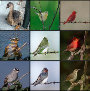
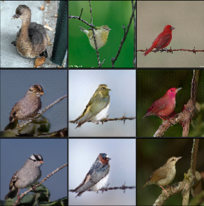
We now push SciMix further by studying versions of the more complex Caltech-UCSD Birds 200 (CUB-200) dataset [32] (6033 pictures of 200 bird species). Given CUB-200 inherently presents few labels, we directly study how fully supervised training benefits from SciMix on low labels settings ( is a standard cross-entropy loss). Furthermore, we take advantage of CUB-200’s higher native resolution to go beyond the limitations of images in CIFAR 10 and SVHN: we use SciMix on commonly studied input sizes (e.g. Tiny ImageNet [38]) and (e.g. STL-10 [39]).

| CUB | ||
|---|---|---|
| Random | ||
Quality of generated hybrids
As can be observed on Fig. 4a, the SciMix autoencoder learns to generate interesting hybrids for different resolutions of the CUB-200 dataset. While the lower resolution hybrids inherit more semantic characteristics of the relevant parent, hybrids still retain semantic patterns tied to the semantic parent’s class.
| Method | CUB-200 | |
|---|---|---|
| Supervised | ||
| SciMix w/ Supervised | ||
Interestingly, SciMix has no difficulty producing hybrids close to their non-semantic parent as can be shown in Tab. 4b by reprising the analysis of the non-semantic transfer rate from Sec. III-B. Analyzing the semantic transfer rate proves more difficult as our best “oracle” classifiers remain unreliable (around accuracy). Nevertheless, the semantic transfer rates in Tab. 4b indicate hybrids generated by SciMix are properly classified by the oracle classifier as having inherited their semantic parent’s class about of the time (orders of magnitude more than attributable to random chance).
Performance gains
Tab. VI shows a fully supervised version of SciMix data augmentation improves supervised models on both and versions of CUB-200. This demonstrates that while SciMix augmentation strongly benefits from a large amount of unlabeled data, it can still generate hybrids diverse enough to benefit training with only a small set of data to generate hybrids from.
IV Conclusion
In conclusion, we propose in this paper a new approach to mixing data augmentation that mixes the semantic content of one sample and the non-semantic content of the other. Making use of advances in style transfer and modular image generation, we train an auto-encoder that learns to extract and combine semantic and non-semantic content from multiple images. Through extensive experiments, we show the intricate hybridization loss we propose leads to the generation of interesting mixed samples. We furthermore demonstrate it is better to use semantic information as an indirect “style code” input to our StyleGan decoder instead of non-semantic information. Afterwards, we prove such data augmentation significantly improves the training of supervised and semi-supervised models when few labels are available.
References
- [1] K. He, X. Zhang, S. Ren, and J. Sun, “Identity mappings in deep residual networks,” in European Conference on Computer Vision, 2016.
- [2] A. Krizhevsky, I. Sutskever, and G. E. Hinton, “Imagenet classification with deep convolutional neural networks,” in Advances in Neural Information Processing Systems, 2012.
- [3] S. Ren, K. He, R. Girshick, and J. Sun, “Faster r-cnn: Towards real-time object detection with region proposal networks,” in Advances in Neural Information Processing Systems, 2015.
- [4] A. Vaswani, N. Shazeer, N. Parmar, J. Uszkoreit, L. Jones, A. N. Gomez, L. u. Kaiser, and I. Polosukhin, “Attention is all you need,” in Advances in Neural Information Processing Systems, 2017.
- [5] Z. He, L. Xie, X. Chen, Y. Zhang, Y. Wang, and Q. Tian, “Data augmentation revisited: Rethinking the distribution gap between clean and augmented data,” Arxiv preprint, 2019.
- [6] T. He, Z. Zhang, H. Zhang, Z. Zhang, J. Xie, and M. Li, “Bag of tricks for image classification with convolutional neural networks,” Computer Vision and Pattern Recognition, 2019.
- [7] O. Chapelle, B. Scholkopf, and A. Zien, Semi-Supervised Learning. The MIT Press, 2006.
- [8] D. Berthelot, N. Carlini, I. Goodfellow, N. Papernot, A. Oliver, and C. A. Raffel, “Mixmatch: A holistic approach to semi-supervised learning,” in Advances in Neural Information Processing Systems, 2019.
- [9] H. Zhang, M. Cisse, Y. N. Dauphin, and D. Lopez-Paz, “mixup: Beyond empirical risk minimization,” in International Conference on Learning Representations, 2018.
- [10] Y. Yang and S. Soatto, “Cutmix: Regularization strategy to train strong classifiers with localizable features,” in International Conference on Computer Vision, 2019.
- [11] L. Carratino, M. Cissé, R. Jenatton, and J.-P. Vert, “On mixup regularization,” in ArXiv preprint, 2020.
- [12] S. Thulasidasan, G. Chennupati, J. A. Bilmes, T. Bhattacharya, and S. Michalak, “On mixup training: Improved calibration and predictive uncertainty for deep neural networks,” in Advances in Neural Information Processing Systems, 2019.
- [13] S. Zagoruyko and N. Komodakis, “Wide residual networks,” in British Machine Vision Conference, 2016.
- [14] K. Sohn, D. Berthelot, C.-L. Li, Z. Zhang, N. Carlini, E. D. Cubuk, A. Kurakin, H. Zhang, and C. Raffel, “Fixmatch: Simplifying semi-supervised learning with consistency and confidence,” Advances in Neural Information Processing Systems, 2020.
- [15] A. Tarvainen and H. Valpola, “Mean teachers are better role models: Weight-averaged consistency targets improve semi-supervised deep learning results,” in Advances in Neural Information Processing Systems, 2017.
- [16] T. Park, J.-Y. Zhu, O. Wang, J. Lu, E. Shechtman, A. Efros, and R. Zhang, “Swapping autoencoder for deep image manipulation,” in Advances in Neural Information Processing Systems, 2020.
- [17] K. He, H. Fan, Y. Wu, S. Xie, and R. Girshick, “Momentum contrast for unsupervised visual representation learning,” in Computer Vision and Pattern Recognition, 2020.
- [18] C. Szegedy, V. Vanhoucke, S. Ioffe, J. Shlens, and Z. Wojna, “Rethinking the inception architecture for computer vision,” in Computer Vision and Pattern Recognition, 2016.
- [19] M.-Y. Liu, T. Breuel, and J. Kautz, “Unsupervised image-to-image translation networks,” in Advances in Neural Information Processing Systems, 2017.
- [20] X. Huang, M.-Y. Liu, S. Belongie, and J. Kautz, “Multimodal unsupervised image-to-image translation,” in European Conference on Computer Vision, September 2018.
- [21] M.-Y. Liu, X. Huang, A. Mallya, T. Karras, T. Aila, J. Lehtinen, and J. Kautz, “Few-shot unsupervised image-to-image translation,” in International Conference on Computer Vision, 2019.
- [22] K. Baek, Y. Choi, Y. Uh, J. Yoo, and H. Shim, “Rethinking the truly unsupervised image-to-image translation,” in International Conference on Computer Vision, 2021.
- [23] X. Huang and S. Belongie, “Arbitrary style transfer in real-time with adaptive instance normalization,” in International Conference on Computer Vision, 2017.
- [24] T. Karras, S. Laine, and T. Aila, “A style-based generator architecture for generative adversarial networks,” in Computer Vision and Pattern Recognition, 2019.
- [25] T. Karras, M. Aittala, S. Laine, E. Härkönen, J. Hellsten, J. Lehtinen, and T. Aila, “Alias-free generative adversarial networks,” in Advances in Neural Information Processing Systems, 2021.
- [26] I. Higgins, L. Matthey, A. Pal, C. Burgess, X. Glorot, M. Botvinick, S. Mohamed, and A. Lerchner, “Beta-vae: Learning basic visual concepts with a constrained variational framework,” in International Conference on Learning Representations, 2017.
- [27] T. Robert, N. Thome, and M. Cord, “Dualdis: Dual-branch disentangling with adversarial learning,” Arxiv preprint, 2019.
- [28] K. Bousmalis, G. Trigeorgis, N. Silberman, D. Krishnan, and D. Erhan, “Domain separation networks,” in Advances in Neural Information Processing Systems, 2016.
- [29] K. Bousmalis, N. Silberman, D. Dohan, D. Erhan, and D. Krishnan, “Unsupervised pixel-level domain adaptation with generative adversarial networks,” in Computer Vision and Pattern Recognition, 2017.
- [30] A. Krizhevsky and G. Hinton, “Learning multiple layers of features from tiny images,” Tech. Rep., 2009.
- [31] Y. Netzer, T. Wang, A. Coates, A. Bissacco, B. Wu, and A. Y. Ng, “Reading digits in natural images with unsupervised feature learning,” in Advances in Neural Information Processing Systems, 2011.
- [32] P. Welinder, S. Branson, T. Mita, C. Wah, F. Schroff, S. Belongie, and P. Perona, “Caltech-UCSD Birds 200,” Tech. Rep., 2010.
- [33] J. Li, C. Xiong, and S. C. Hoi, “Comatch: Semi-supervised learning with contrastive graph regularization,” in International Conference on Computer Vision, 2021.
- [34] B. Zhang, Y. Wang, W. Hou, H. Wu, J. Wang, M. Okumura, and T. Shinozaki, “Flexmatch: Boosting semi-supervised learning with curriculum pseudo labeling,” in Advances in Neural Information Processing Systems, 2021.
- [35] T. Karras, S. Laine, M. Aittala, J. Hellsten, J. Lehtinen, and T. Aila, “Analyzing and improving the image quality of stylegan,” in Computer Vision and Pattern Recognition, June 2020.
- [36] Y. Yang and S. Soatto, “Fda: Fourier domain adaptation for semantic segmentation,” in Computer Vision and Pattern Recognition, 2020.
- [37] H. Inoue, “Data augmentation by pairing samples for images classification,” Arxiv preprint, 2018.
- [38] P. Chrabaszcz, I. Loshchilov, and F. Hutter, “A downsampled variant of imagenet as an alternative to the cifar datasets,” Arxiv preprint, 2017.
- [39] A. Coates, A. Ng, and H. Lee, “An analysis of single-layer networks in unsupervised feature learning,” in International Conference on Artificial Intelligence and Statistics, 2011.