Large-Signal Stability Guarantees for
Cycle-by-Cycle Controlled DC-DC Converters

Abstract

Stability guarantees are critical for cycle-by-cycle controlled dc-dc converters in consumer electronics and energy storage systems. Traditional stability analysis on cycle-by-cycle dc-dc converters is incomplete because the inductor current ramps are considered fixed; but instead, inductor ramps are not fixed because they are dependent on the output voltage in large-signal transients. We demonstrate a new large-signal stability theory which treats cycle-by-cycle controlled dc-dc converters as a particular type of feedback interconnection system. An analytical and practical stability criterion is provided based on this system. The criterion indicates that the $L/R$ and $RC$ time constants are the design parameters which determine the amount of coupling between the current ramp and the output voltage.

I Introduction

Cycle-by-cycle controlled dc-dc converters are widely used in PoL (point-of-load) regulators [1], VRMs (voltage regulation modules) [2], battery chargers [3], and LiDAR power supplies [4] because of its faster transient response compared to the traditional averaging-based control [5]. However, the well-known averaging theory cannot model the fast switching-frequency-scale dynamics of cycle-by-cycle controlled dc-dc converters due to the slow-varying perturbation assumption. The switching-synchronized sampled-state space (5S) model is an accurate and tractable alternative [6].

In comparison to the bilinear nonlinearity in the averaging model, the converter model in 5S illustrates more complicated nonlinear behaviors. While the small-signal stability in 5S has been widely discussed in [6], the large-signal stability of cycle-by-cycle controlled dc-dc converters has not been adequately addressed.

This paper focuses on one of the most widely-used cycle-by-cycle controlled dc-dc converters — current-mode dc-dc converters, which have a number of varieties including constant on-time control [7], constant off-time control [8], and fixed-frequency peak current control [9]. In the existing large-signal stability analysis for current-mode converters, the current block and voltage block shown in Fig. 1 in current-mode dc-dc converters are considered decoupled and are designed separately. The stability of the current block, which is referred to “fast-scale stability”, was studied by assuming the rising ramp and falling ramp of the inductor current are fixed as $m_{1}$ and $m_{2}$ [10]. The stability of the voltage block, which is referred to “slow-scale stability”, was studied by utilizing averaging theory because of negligible voltage ripple and treating the current block as a controlled current source.

However, during large-signal transients, the output voltage significantly changes, hence the inductor current ramp changes every switching cycle. The cycle-varying inductor current ramp affects the amount of charge pumped into the output, and ultimately affects the output voltage dynamics. The traditional large-signal stability analysis of the current block, which fully neglects the voltage block and assumes a fixed inductor current ramp, cannot guarantee the stability of the current block for large-signal transients.

To address this deficiency in the large-signal stability theory of current-mode dc-dc converters, we develop a new large-signal stability theory which models the current-mode buck converter as a feedback connection system in 5S shown in Fig. 1. Several discrete-time robust control tools, including small-gain theorem, dissipativity theory, and Lure system theory are utilized to rigorously study the stability of the resulting discrete-time nonlinear system.

This paper is organized as the following: (i) Section I introduces the paper; (ii) Section II develops the large-signal models for the current block and voltage block of a current-mode buck converter using constant on-time control; (iii) the ultimate goal, which is illustrated in Section III, is to derive the large-signal stability guarantees for current mode dc-dc converters; (iv) Section IV concludes the paper.

Figure 1: The current block and voltage block are coupled if the inductor current ramp is cycle-varying.

II 5S Modeling of Constant On-Time
Buck Converter

II-A Converters, Systems, and Definitions

Consider a class $\Sigma$ buck converter [6] using constant on-time current-mode control is illustrated in Fig. 2.

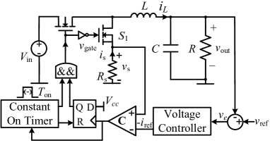
Figure 2: Schematic diagram of a digitally-controlled current-mode constant on-time buck converter.

The inductor current and capacitor voltage trajectories are shown in Fig. 3. $V_{\text{in}}$ and $T_{\text{on}}$ are the input voltage and constant on time, respectively. According to the cycle-by-cycle control law in [6], the output voltage is sampled during the on-time, once per switching cycle. The sampling time point for $v[n]$ can be expressed as the convex combination of the time of the inductor current valley $t_{v}[n]$ and the time for the inductor current peak $t_{p}[n]$.

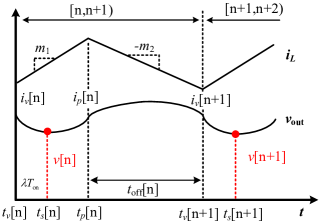
Figure 3: Constant on-time buck converter using cycle-by-cycle current-mode control.

$$t_{s}[n]=\lambda t_{v}[n-1]+(1-\lambda)t_{p}[n],$$ (1)

the parameter $\lambda$ can be chosen to be from 0 to 1.

The slopes of the rising and falling ramps of the inductor current are denoted by $m_{1}[n]$ and $m_{2}[n]$

$$m_{1}[n] =\frac{V_{\text{in}}-v[n]}{L},\quad m_{2}[n]=\frac{v[n]}{L}.$$ (2)

We introduce the one-cycle-delayed valley current sequence $\{i_{v}^{p}[n]\}$ as

$$i_{v}^{p}[n+1]\triangleq i_{v}[n].$$ (3)

We denote the equilibrium of the system by $v_{out}[n]=V_{\text{out}}$, $i_{v}[n]=I_{v}$, $i_{v}^{p}[n]=I_{v}$, and $t_{\text{off}}[n]=T_{\text{off}}$. The interference signal in the inductor current measurement is denoted by $w(t)$ [11]. The equilibrium is defined by the following equations:

$$I_{v} \triangleq\frac{V_{\text{out}}}{R}-\frac{1}{2}\frac{V_{\text{in}}-V_{\text{out}}}{L}\,T_{\text{on}},\quad I_{v}=I_{c}-w(T_{\text{off}}),$$ (4a)

$$T_{\text{off}} \triangleq\frac{V_{\text{in}}-V_{\text{out}}}{V_{\text{out}}}\,T_{\text{on}},\quad T_{s}^{\text{ss}}\triangleq T_{\text{on}}+T_{\text{off}},$$ (4b)

II-B Current Block Modeling

According to [11], the large-signal dynamical model (translated to the origin) of the current block follows

$$\tilde{i}_{v}^{p}[n+1] =\tilde{i}_{v}^{p}[n]-\frac{\tilde{v}[n]}{L}\,\,T_{\text{on}}-\frac{\tilde{v}[n]}{L}\,\,T_{\text{off}}-\frac{v[n]}{L}\,\,\tilde{t}_{\text{off}}[n],$$ (5a)

$$\tilde{i}_{v}^{p}[n+1] =\tilde{i}_{c}[n]-\psi(\tilde{t}_{\text{off}}[n]),$$ (5b)

where the translated variables $\tilde{v}[n]$, $\tilde{i}_{v}^{p}[n]$, $\tilde{t}_{\text{off}}[n]$, and $\psi$ satisfy

$$\tilde{v}[n] =v[n]-V_{\text{out}},\quad\tilde{i}_{v}^{p}[n]=i_{v}^{p}[n]-I_{v},$$ (6a)

$$\tilde{t}_{\text{off}}[n] =t_{\text{off}}[n]-T_{\text{off}},\quad\psi(x)=w(x+T_{\text{off}})-w(x).$$ (6b)

From (5), the current control block diagram can be represented by Fig. 4.

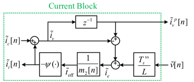
Figure 4: Current block diagram of current-mode buck converter using constant on-time.

II-C Voltage Block Modeling

From [6], constant on-time current-mode buck converters have the following two properties: (1) the output $RC$-filter time constant is much greater than the switching period; (2) the output voltage has a small ripple so the inductor current can be considered as a cycle-varying piecewise linear (ramp) waveform. Property (1) implies

$$\frac{T_{s}[n]}{RC}\ll 1,$$ (7)

where $T_{s}$ is the switching period at the $n^{\text{th}}$ switching cycle. Property (2) implies that the quasi-steady state discharging of the capacitor, i.e. the discharging current to the load, can be treated as constant throughout a given switching cycle, and the small output-voltage ripple

$$\frac{T_{s}[n]\,T_{\text{on}}}{2LC} \ll 1.$$ (8)

The large-signal dynamical model (translated to the origin) of the voltage block follows [6]:

$$\tilde{v}[n+1]=\,\, \tilde{v}[n]+\frac{1}{C}\left(\sum_{j=1}^{3}\tilde{Q}^{(j)}_{\text{in}}[n]-\tilde{Q}_{\text{out}}[n]\right),$$ (9a)

$$\tilde{Q}^{(1)}_{\text{in}}[n]=\,\, (1-\lambda)T_{\text{on}}\tilde{i}_{v}^{p}[n]-\frac{1-\lambda^{2}}{2}\frac{\tilde{v}[n]}{L}\;T^{2}_{\text{on}},$$ (9b)

$$\tilde{Q}^{(2)}_{\text{in}}[n]=\,\, \frac{1}{2}\left(\tilde{i}_{v}^{p}[n]-\frac{\tilde{v}[n]}{L}\;T_{\text{on}}+\tilde{i}_{v}^{p}[n+1]\right)t_{\text{off}}[n]$$

$$+\left(I_{v}+\frac{M_{1}T_{\text{on}}}{2}\right)\tilde{t}_{\text{off}}[n],$$ (9c)

$$\tilde{Q}^{(3)}_{\text{in}}[n]=\,\, \lambda T_{\text{on}}i_{v}^{p}[n+1]-\frac{\lambda^{2}}{2}\frac{\tilde{v}[n]}{L}\;T^{2}_{\text{on}},$$ (9d)

$$\tilde{Q}_{\text{out}}[n]=\,\, \frac{\tilde{v}[n]}{R}\left(T_{\text{on}}+t_{\text{off}}[n]\right)+\frac{V_{\text{out}}}{R}\;\tilde{t}_{\text{off}}[n].$$ (9e)

To prevent the switching transient from disturbing the valley current detection denoted by the sense voltage $v_{s}$ in Fig. 2, the time-varying off-time is bounded from below [6]. To avoid the misdetection of the valley current event, the time-varying off-time is bounded from above by

$$T^{\text{min}}_{\text{off}}\leq t_{\text{off}}[n]\leq T^{\text{max}}_{\text{off}}.$$ (10)

III Stability and Control Performance Analysis of Constant On-Time Buck Converters

III-A Current Block

To calculate the $\mathcal{L}_{2}$ gain from $\tilde{v}[n]$ to $\tilde{i}_{v}^{p}[n]$, denoted by $\Gamma_{v\to i}$, we introduce the following dissipativity theory.

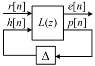
Figure 5: Linear fractional transformed system.

If the system can be expressed in $F_{u}(L,\Delta)$ form [12], as shown in Fig. 5, then the state-space representation of $F_{u}(L,\Delta)$ is

$$x[n+1] =Ax[n]+B_{1}h[n]+B_{2}r[n],$$ (11a)

$$p[n] =C_{1}x[n]+D_{11}h[n]+D_{12}r[n],$$ (11b)

$$e[n] =C_{2}x[n]+D_{21}h[n]+D_{22}r[n],$$ (11c)

$$h[n] =\Delta\,\left(p[n]\right),$$ (11d)

the upper bound of the $\mathcal{L}_{2}$ gain can be calculated as

Theorem 1.

Assume $\Delta\mathrel{\mathop{\ordinarycolon}}\mathbb{R}\rightarrow\mathbb{R}$ is an $[\hat{\alpha},\hat{\beta}]$ sector-bounded nonlinearity. Also, assume $F_{u}(L,\Delta)$ is well-posed. If $\exists\,P>0$, $\lambda\geq 0$, and $\hat{\gamma}>0$ such that

$$\begin{bmatrix}A^{T}PA-P&A^{T}PB_{1}&A^{T}PB_{2}\\ B_{1}^{T}PA&B_{1}^{T}PB_{1}&B_{1}^{T}PB_{2}\\ B_{2}^{T}PA&B_{2}^{T}PB_{1}&B_{2}^{T}PB_{2}-\hat{\gamma}^{2}I\end{bmatrix}$$

$$+\lambda\begin{bmatrix}C_{1}&D_{11}&D_{12}\\ 0&I&0\end{bmatrix}^{T}\begin{bmatrix}-\hat{\alpha}\hat{\beta}&\frac{\hat{\alpha}+\hat{\beta}}{2}\\ \frac{\hat{\alpha}+\hat{\beta}}{2}&-1\end{bmatrix}\begin{bmatrix}C_{1}&D_{11}&D_{12}\\ 0&I&0\end{bmatrix}$$

$$+\begin{bmatrix}C_{2}^{T}\\ D_{21}^{T}\\ D_{22}^{T}\end{bmatrix}\begin{bmatrix}C_{2}&D_{12}&D_{22}\end{bmatrix}<0,$$ (12)

then $\|F_{u}(L,\Delta)\|\leq\hat{\gamma}$.

Proof.

Let $r\in L_{2}$ be any input and assume $x[0]=0$. Let $(x,p,h,e)$ be the resulting solutions for this input $r$.

Multiply the left and right of (1) by $\left[x[n]^{T}\,\,p[n]^{T}\,\,r[n]^{T}\right]$ and its transpose to obtain

$$V(x[n+1])-V(x[n])-\hat{\gamma}^{2}r[n]^{T}r[n]$$

$$+\Lambda\begin{bmatrix}p[n]\\ h[n]\end{bmatrix}^{T}\begin{bmatrix}-\hat{\alpha}\hat{\beta}&\frac{\hat{\alpha}+\hat{\beta}}{2}\\ \frac{\hat{\alpha}+\hat{\beta}}{2}&-1\end{bmatrix}\begin{bmatrix}p[n]\\ h[n]\end{bmatrix}+e[n]^{T}e[n]<0,$$ (13)

where the storage function $V(x)$ is defined as $V(x)\triangleq x^{T}Px$.

By summing up both sides of (III-A) from $n=0$ to $n=N$, we have

$$V(x[N+1])-V(x[0])-\hat{\gamma}^{2}\sum_{n=0}^{N}r[n]^{T}r[n]$$

$$+\Lambda\sum_{n=0}^{N}\begin{bmatrix}p[n]\\ h[n]\end{bmatrix}^{T}\begin{bmatrix}-\hat{\alpha}\hat{\beta}&\frac{\hat{\alpha}+\hat{\beta}}{2}\\ \frac{\hat{\alpha}+\hat{\beta}}{2}&-1\end{bmatrix}\begin{bmatrix}p[n]\\ h[n]\end{bmatrix}+\sum_{n=0}^{N}e[n]^{T}e[n]<0.$$ (14)

(III-A) can be equivalently expressed as

$$V(x[N+1])-V(x[0])+\sum_{n=0}^{N}e[n]^{T}e[n]-\sum_{n=0}^{N}\hat{\gamma}^{2}r[n]^{T}r[n]$$

$$+\Lambda\sum_{n=0}^{N}\left(h[n]-\hat{\alpha}p[n]\right)\left(\hat{\beta}p[n]-h[n]\right)<0.$$ (15)

$V(x[N+1])\geq 0$ because $P>0$. $V(x[0])=0$ because $x[0]=0$. $h[n]\geq\hat{\alpha}p[n]$ and $\hat{\beta}p[n]\leq h[n]$ because of the sector-bounded nonlinearity. The last term in (III-A) is non-negative because of both the sector-bounded nonlinearity and positive scalar term $\Lambda$. Therefore, (III-A) implies

$$\sum_{n=0}^{N}e[n]^{T}e[n]<\sum_{n=0}^{N}\hat{\gamma}^{2}r[n]^{T}r[n].$$ (16)

Take $N\rightarrow\infty$ to show $\|e\|_{2}^{2}<\hat{\gamma}^{2}\|r\|_{2}^{2}$. In all, the $\mathcal{L}_{2}$ norm of $F_{u}(L,\Delta)$ is bounded by $\hat{\gamma}$. ∎

We reformulate the current block in a unitless $F_{u}(L,\Delta)$ form as

$$\tilde{i}_{v}^{p}[n+1] =\tilde{i}_{i}[n],\quad\tilde{i}_{e}[n]=\tilde{i}_{v}^{p}[n]-\tilde{i}_{i}[n]+\tilde{u}[n],$$ (17a)

$$\tilde{i}_{v}^{p}[n] =\tilde{i}_{v}^{p}[n],\quad\tilde{i}_{i}[n]=\Delta(\tilde{i}_{e}[n]),$$ (17b)

where

$$\tilde{u}[n]=\frac{T^{\text{ss}}_{s}}{L}\tilde{v}[n],\quad\Delta(z)=-\psi\left(\frac{z}{m_{2}[n]}\right),$$ (18)

and $\Delta(z)\in[\hat{\alpha},\hat{\beta}]$ is a sector-bounded time-varying nonlinearity.

From Theorem 1, the gain $\hat{\gamma}$ of unitless $F_{u}(L,\Delta)$ form can be obtained from following optimization problem:

$$\underset{\hat{\gamma},\lambda,P}{\mathrm{min}} \,\,\,\hat{\gamma}^{2}$$ (19a)

subject to $$\,\,P>0,\,\lambda\geq 0,\,\hat{\gamma}>0,$$ (19b)

$$\lambda\begin{bmatrix}-\hat{\alpha}\hat{\beta}&\hat{\alpha}\hat{\beta}+\frac{\hat{\alpha}+\hat{\beta}}{2}&-\hat{\alpha}\hat{\beta}\\ \hat{\alpha}\hat{\beta}+\frac{\hat{\alpha}+\hat{\beta}}{2}&-2\hat{\alpha}\hat{\beta}-\hat{\alpha}-\hat{\beta}&\hat{\alpha}\hat{\beta}+\frac{\hat{\alpha}+\hat{\beta}}{2}\\ -\hat{\alpha}\hat{\beta}&\hat{\alpha}\hat{\beta}+\frac{\hat{\alpha}+\hat{\beta}}{2}&-\hat{\alpha}\hat{\beta}\end{bmatrix}$$

$$+\begin{bmatrix}1-P&0&0\\ 0&P&0\\ 0&0&-\hat{\gamma}^{2}\end{bmatrix}<0.$$ (19c)

Problem (19) is in linear matrix inequality (LMI) form, hence is convex and the global minimum exists. By applying an LMI solver (e.g. CVX), we obtain the gain of system (17) as a function of the sector bounds,

$$\hat{\gamma}=g(\hat{\alpha},\hat{\beta}).$$ (20)

If there is no interference, $\hat{\alpha}=\hat{\beta}=0$, system (17) has zero gain, and voltage doesn’t affect the current. As $\hat{\alpha}$ decreases and $\hat{\beta}$ increases, system (17) has larger gain, as shown in Fig. 6.

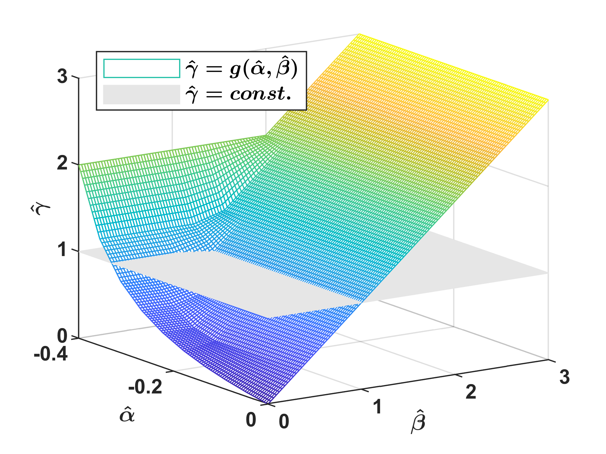
Figure 6: Gain of system (17) as a function of sector bounds. For no interference, $\hat{\alpha}=\hat{\beta}=0$, system (17) has zero gain, and voltage does not affect the current. As $\hat{\alpha}$ decreases and $\hat{\beta}$ decreases, system (17) has larger gain.

The following corollary follows Theorem  1:

Corollary 1.

Given the class $\Sigma$ buck converter modeled by [6], the $\mathcal{L}_{2}$ gain from the sampled output voltage sequence $\{\tilde{v}[n]\}$ to one-cycle-delayed inductor current sequence $\{\tilde{i}^{p}_{v}[n]\}$ is bounded from above by

$$\Gamma_{v\to i}\leq\frac{T_{s}^{\text{ss}}}{L}g(\hat{\alpha},\hat{\beta}),$$ (21)

where $T_{s}^{\text{ss}}$ is the steady-state switching period,

$$T_{s}^{\text{ss}} \triangleq T_{\text{on}}+T_{\text{off}}.$$ (22)

III-B Voltage Block

The voltage dynamics, which is described by the nonlinear time-invariant system (9), is a nonlinear system with quadratic and fractional nonlinearities. A straightforward mathematical tool does not exist to analytically study the stability and calculate the $\mathcal{L}_{2}$ gain in closed form. The algorithmic method only applies to a buck converter with specific $L$, $C$, and $R$. Therefore, it is difficult to generalize the algorithmic methods and give engineering intuitions to the designers.

We solve this challenge by taking advantage of the inherent physical constraint of constant on-time buck converters that the cycle-varying off-time is bounded by (10).

Theorem 2.

Given the class $\Sigma$ buck converter modeled by [6], the $\mathcal{L}_{2}$ gain from the one-cycle-delayed inductor current sequence $\{\tilde{i}^{p}_{v}[n]\}$ to sampled output voltage sequence $\{\tilde{v}[n]\}$ is bounded from above by

$$\Gamma_{i\to v} \leq\frac{R}{\left(1+\frac{T_{\text{on}}}{2\tau_{2}}\right)}\frac{T_{s}^{\text{max}}}{T_{s}^{\text{min}}},$$ (23)

where $T_{s}^{\text{min}}$ and $T_{s}^{\text{max}}$ are the shortest switching period and longest switching period, respectively, and $\tau_{2}$ is the $L/R$ time constant,

$$T_{s}^{\text{max}} \triangleq T_{\text{on}}+T_{\text{off}}^{\text{max}},\quad T_{s}^{\text{min}}\triangleq T_{\text{on}}+T_{\text{off}}^{\text{min}},\quad\tau_{2}\triangleq\frac{L}{R}.$$ (24)

Proof.

(i) Voltage Block Model Reformulation
The nonlinear time-invariant system (9) can be transformed to the following linear time-varying system

$$\tilde{v}[n+1] =\alpha[n]\,\tilde{v}[n]+\beta[n]\,\tilde{i}_{v}^{p}[n]+\gamma[n]\,\tilde{i}_{v}^{p}[n+1],$$ (25a)

$$\alpha[n] =1-\frac{T_{\text{on}}+t_{\text{off}}[n]}{RC}-\frac{T_{\text{on}}\left(T_{\text{on}}+t_{\text{off}}[n]\right)}{2LC},$$ (25b)

$$\beta[n] =\frac{1}{C}\left((1-\lambda)T_{\text{on}}+\frac{1}{2}t_{\text{off}}[n]\right),$$ (25c)

$$\gamma[n] =\frac{1}{C}\left(\lambda T_{\text{on}}+\frac{1}{2}t_{\text{off}}[n]\right).$$ (25d)

From (10), the time-varying coefficients are bounded by

$$0<\alpha[n] \leq\alpha_{\text{max}}=1-\frac{T_{s}^{\text{min}}}{RC}-\frac{T_{\text{on}}T_{s}^{\text{min}}}{2LC},$$ (26a)

$$0<\beta[n] \leq\beta_{\text{max}}=\frac{1}{C}\left((1-\lambda)T_{\text{on}}+\frac{1}{2}T_{\text{off}}^{\text{max}}\right),$$ (26b)

$$0<\gamma[n] \leq\gamma_{\text{max}}=\frac{1}{C}\left(\lambda T_{\text{on}}+\frac{1}{2}T_{\text{off}}^{\text{max}}\right).$$ (26c)

We transform the linear time-varying system into standard state-space representation

$$\tilde{v}[n+1] =\alpha[n]q[n]+\left(\beta[n]+\alpha[n]\gamma[n]\right)\tilde{i}_{v}^{p}[n],$$ (27a)

$$\tilde{v}[n] =q[n]+\gamma[n]\tilde{i}_{v}^{p}[n].$$ (27b)

(ii) Gain Estimation
We utilize a storage function $\mathcal{V}[n]=q^{2}[n]$ to calculate the $\mathcal{L}_{2}$ gain of the dynamical system (27a)

$$\mathcal{V}[n+1]-\mathcal{V}[n]=q^{2}[n+1]-q^{2}[n].$$ (28)

From the Cauchy-Schwartz Inequality, given any $\mu_{1}>0$, $q^{2}[n+1]$ can be bounded from the above by

$$q^{2}[n+1]$$

$$= \,\,\left(\alpha[n]q[n]+\left(\beta[n]+\alpha[n]\gamma[n]\right)\tilde{i}_{v}^{p}[n]\right)^{2}$$

$$\leq \,\,\left(\alpha^{2}[n]q^{2}[n]+(\beta[n]+\alpha[n]\gamma[n])^{2}\frac{(\tilde{i}_{v}^{p}[n])^{2}}{\mu_{1}}\right)\left(1+\mu_{1}\right).$$ (29)

We let $\mu_{1}=(1-\alpha[n])(\alpha[n])^{-1}$. It can be verified that $\mu_{1}>0$ from (7) and (8)

$$q^{2}[n+1]\leq\alpha[n]q^{2}[n]+\frac{\left(\beta[n]+\alpha[n]\gamma[n]\right)}{1-\alpha[n]}(\tilde{i}_{v}^{p}[n])^{2}.$$ (30)

Substitute (30) to (28),

$$\mathcal{V}[n+1]-\mathcal{V}[n]\leq$$

$$\frac{\left(\beta[n]+\alpha[n]\gamma[n]\right)^{2}}{1-\alpha[n]}\;(\tilde{i}_{v}^{p}[n])^{2}-(1-\alpha[n])q^{2}[n]\leq$$

$$\frac{\left(\beta_{\text{max}}+\alpha_{\text{max}}\gamma_{\text{max}}\right)^{2}}{1-\alpha_{\text{max}}}\;(\tilde{i}_{v}^{p}[n])^{2}-(1-\alpha_{\text{max}})q^{2}[n]=$$

$$(1-\alpha_{\text{max}})\left(\frac{\left(\beta_{\text{max}}+\alpha_{\text{max}}\gamma_{\text{max}}\right)^{2}}{(1-\alpha_{\text{max}})^{2}}\;(\tilde{i}_{v}^{p}[n])^{2}-q^{2}[n]\right).$$ (31)

Summing both sides of the inequality for all $n$ yields

$$\mathcal{V}(\infty)-\mathcal{V}(1)\leq(1-\alpha_{\text{max}})\left(\Gamma_{1}^{2}\|\tilde{i}_{v}^{p}\|_{2}^{2}-\|q\|_{2}^{2}\right),$$ (32)

where $\|\cdot\|_{2}$ is the $\mathcal{L}_{2}$ norm and

$$\Gamma_{1}=\frac{\left(\beta_{\text{max}}+\alpha_{\text{max}}\gamma_{\text{max}}\right)}{(1-\alpha_{\text{max}})}.$$ (33)

The $\mathcal{L}_{2}$ norm of $q[n]$ can be bounded by

$$\|q\|^{2} \leq\Gamma_{1}^{2}\|\tilde{i}_{v}^{p}\|_{2}^{2}+\frac{V(1)-V(\infty)}{(1-\alpha_{\text{max}})}\leq\Gamma_{1}^{2}\|\tilde{i}_{v}^{p}\|_{2}^{2}+\frac{V(1)}{(1-\alpha_{\text{max}})}.$$ (34)

By definition, the $\mathcal{L}_{2}$ gain of system (27a) is bounded from above by $\Gamma_{1}$.

The $\mathcal{L}_{2}$ gain of the system (27b) can be obtained from the Cauchy-Schwartz Inequality as

$$\tilde{v}^{2}[n]=(q[n]+\gamma[n]\tilde{i}_{v}^{p}[n])^{2}\leq$$

$$\left(q^{2}[n]+\gamma^{2}[n](\tilde{i}_{v}^{p}[n])^{2}\frac{\Gamma_{1}}{\gamma[n]}\right)\left(1+\frac{\gamma[n]}{\Gamma_{1}}\right)\leq$$

$$\left(\Gamma_{1}+\gamma[n]\right)\Gamma_{1}(\tilde{i}_{v}^{p}[n])^{2}+\left(\Gamma_{1}+\gamma[n]\right)\gamma[n](\tilde{i}_{v}^{p}[n])^{2}\leq$$

$$\left(\Gamma_{1}+\gamma_{\text{max}}\right)(\tilde{i}_{v}^{p}[n])^{2}.$$ (35)

Summing both sides of the inequality for all $n$ yields the $\mathcal{L}_{2}$ gain of the system (27b)

$$\|v\|_{2}\leq\left(\Gamma_{1}+\gamma_{\text{max}}\right)\|\tilde{i}_{v}^{p}\|_{2}.$$ (36)

By (33), the $\mathcal{L}_{2}$ gain of the voltage block can be bounded from above

$$\Gamma_{i\to v} \leq\Gamma_{1}+\gamma_{\text{max}}=\frac{\beta_{\text{max}}+\gamma_{\text{max}}}{1-\alpha_{\text{max}}}=\frac{R}{\left(1+\frac{T_{\text{on}}}{2\tau_{2}}\right)}\frac{T_{s}^{\text{max}}}{T_{s}^{\text{min}}},$$ (37)

where $T_{s}^{\text{min}}$ and $T_{s}^{\text{max}}$ are the shortest switching period and longest switching period, respectively, and $\tau_{2}$ is the $L/R$ time constant. ∎

III-C Overall System

From the Small Gain Theorem [13], the current-mode buck converter is finite-gain $\mathcal{L}_{2}$ stable if

$$\Gamma_{i\to v}\cdot\Gamma_{v\to i}<1.$$ (38)

By substituting (21) and (37) into (38), (38) is equivalent to

$$g(\hat{\alpha},\hat{\beta})<\left(\tau_{2}+\frac{T_{\text{on}}}{2}\right)\frac{T_{s}^{\text{min}}}{T_{s}^{\text{max}}}\frac{1}{T_{s}^{ss}},$$ (39)

where $T_{s}^{\text{min}}$, $T_{s}^{\text{max}}$, and $T_{s}^{\text{ss}}$ are the shortest switching period, longest switching period, and steady-state switching period, respectively.

Because both current and voltage blocks are zero state observable [14], finite-gain $\mathcal{L}_{2}$ stability implies the current-mode buck converter is large-signal asymptotically stable. The following corollary follows from Corollary 2:

Corollary 2.

The current control loop of class $\Sigma$ buck converters using constant on-time current-mode control is globally asymptotically stable if

$$g(\hat{\alpha},\hat{\beta})<\left(\tau_{2}+\frac{T_{\text{on}}}{2}\right)\frac{T_{s}^{\text{min}}}{T_{s}^{\text{max}}}\frac{1}{T_{s}^{ss}},$$ (40)

$$T_{s}^{\text{max}}\left(1+\frac{T_{\text{on}}}{2\tau_{2}}\right)<\tau_{1},$$ (41)

where $g(\hat{\alpha},\hat{\beta})$ follows (20), $T_{s}^{\text{min}}$ and $T_{s}^{\text{max}}$ are the shortest switching period and longest switching period, respectively, $\tau_{1}$ is the $RC$ time constant, and $\tau_{2}$ is the $L/R$ time constant,

$$T_{s}^{\text{max}} \triangleq T_{\text{on}}+T_{\text{off}}^{\text{max}},\quad T_{s}^{\text{min}}\triangleq T_{\text{on}}+T_{\text{off}}^{\text{min}},$$ (42)

$$\tau_{1} \triangleq RC,\quad\tau_{2}\triangleq\frac{L}{R}.$$ (43)

IV Modeling and Stability of Constant Off-Time Boost Converter

The modeling and stability of the constant off-time boost converters can be studied in the similar manners.

IV-A Current-Mode Boost Converter Using Constant Off-Time

Consider a class $\Sigma$ boost converter using constant off-time defined in [6], the on-time in steady state is denoted by $T_{\text{off}}$. The time-varying on-time is bounded from above by

$$T^{\text{min}}_{\text{on}}\leq t_{\text{on}}[n]\leq T^{\text{max}}_{\text{on}}.$$ (44)

The large-signal stability guarantee is shown in Proposition 1. The detailed proof can be found in [15]:

Proposition 1.

The current control loop of the class $\Sigma$ boost converter using constant off-time control is globally asymptotically stable

(i) if $\left((1-\lambda)T_{\text{off}}+\frac{V_{\text{out}}L}{V_{\text{in}}R}\right)\left(1-\frac{T_{s}^{\text{ss}}}{RC}-\frac{T_{s}^{\text{max}}}{RC}-\frac{T^{2}_{\text{off}}}{2LC}\right)+\left(\lambda T_{\text{off}}-\frac{V_{\text{out}}L}{V_{\text{in}}R}\right)\geq 0$  and

$$g(\hat{\alpha},\hat{\beta}) \leq\frac{1}{2}+\tau_{2}\left(\frac{T_{s}^{\text{ss}}+T_{s}^{\text{min}}}{T_{s}^{\text{ss}}T_{\text{off}}}\right);$$ (45)

or (ii) if $\left((1-\lambda)T_{\text{off}}+\frac{V_{\text{out}}L}{V_{\text{in}}R}\right)\left(1-\frac{T_{s}^{\text{ss}}}{RC}-\frac{T_{s}^{\text{max}}}{RC}-\frac{T^{2}_{\text{off}}}{2LC}\right)+\left(\lambda T_{\text{off}}-\frac{V_{\text{out}}L}{V_{\text{in}}R}\right)<0$  and

$$g(\hat{\alpha},\hat{\beta})\leq$$ (46)

$$\frac{2\tau_{2}\left(T_{s}^{\text{min}}+T_{s}^{\text{ss}}\right)+T_{\text{off}}^{2}}{2\tau_{2}\left(T_{s}^{\text{max}}+T_{s}^{\text{ss}}\right)+T_{\text{off}}^{2}}\frac{2\tau_{1}-T_{s}^{\text{ss}}-T_{s}^{\text{max}}-\frac{T_{\text{off}}^{2}}{2\tau_{2}}}{2\frac{V_{\text{out}}}{V_{\text{in}}}+(1-2\lambda)\frac{T_{\text{off}}}{\tau_{2}}}T_{\text{off}};$$

where $g(\hat{\alpha},\hat{\beta})$ follows Fig. 6, $T_{s}^{\text{min}}$ and $T_{s}^{\text{max}}$ are the shortest switching period and longest switching period, respectively, $\tau_{1}$ is the $RC$ time constant, and $\tau_{2}$ is the $L/R$ time constant,

$$T_{s}^{\text{max}} \triangleq T_{\text{on}}+T_{\text{off}}^{\text{max}},$$ (47)

$$T_{s}^{\text{min}} \triangleq T_{\text{on}}+T_{\text{off}}^{\text{min}},$$ (48)

$$\tau_{1} \triangleq RC,\quad\tau_{2}\triangleq\frac{L}{R}.$$ (49)

V Simulation Validation

The proposed stability criterion was validated by a high-fidelity switch-circuit simulation model in MATLAB/Simulink. The parameters of the constant on-time buck converter system in the validation are shown in Table I. Two case studies were performed with different resistive load conditions as shown in Table II. The inductor currents were controlled so that the steady-state output voltages were kept the same. The inadequacy of the existing stability criterion [11] is illustrated for Case 1 in Fig.  7. The proposed stability criterion, which guarantees the large-signal stability of the power converter system, is demonstrated for Case 2 in Fig. 8.

TABLE I: Design Parameters of the Constant On-Time Current-Mode Buck Converter

Param.	Values	Param.	Values	Param.	Values
$\boldsymbol{V_{\textbf{in}}}$	12 V	$\boldsymbol{L}$	240 nH	$\boldsymbol{T_{\textbf{on}}}$	100 ns
$\boldsymbol{V_{\textbf{out}}}$	2.2 V	$\boldsymbol{C}$	100 $\mu$F	$\boldsymbol{R_{s}}$	10 m$\Omega$

TABLE II: Validations of the proposed stability criterion (39)

Case	R	$\mathbf{\emph{I}_{\text{cmd}}}$	$\mathbf{|\hat{\alpha}|}$	Corollary 1 [11]	(39)
1	$0.4\,\Omega$	4.5 A	0.48	$|\hat{\alpha}|<0.5$	$|\hat{\alpha}|<0.24$
2	$0.05\,\Omega$	43 A	0.3	$|\hat{\alpha}|<0.5$	$|\hat{\alpha}|<0.44$

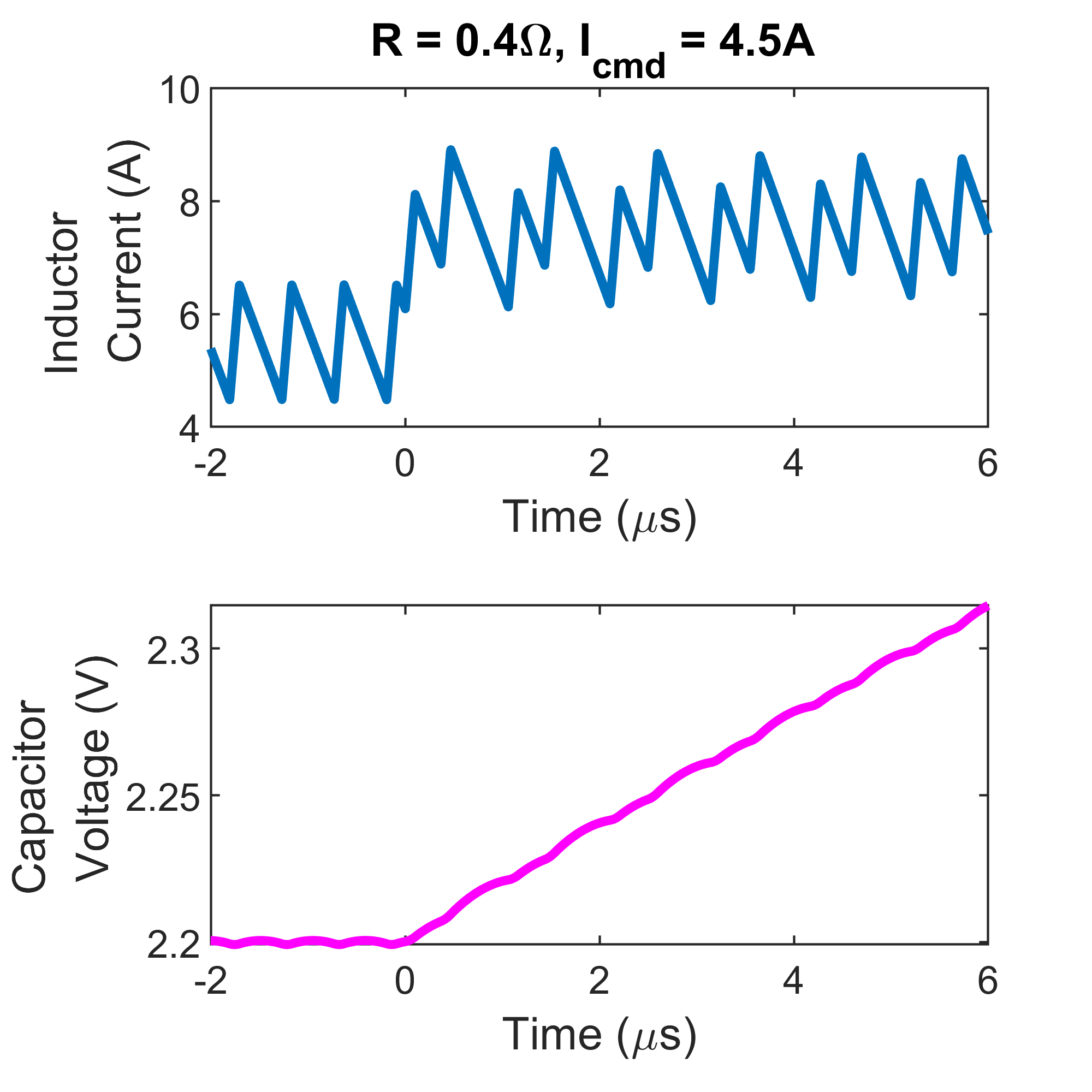
Figure 7: In case study 1, for $R=0.4\,\Omega$ and $I_{\text{cmd}}=4.5\,\text{A}$, according to stability criterion (39), the current control loop is stable if the interference is sector-bounded by $|\hat{\alpha}|<0.24$. In the Simulink simulation, interference with sector bound $|\hat{\alpha}|=0.48$ is added to the inductor current measurement; the inductor current waveform is unstable for a current step. This result shows that the expectation of stability from pre-existing theory that ignores the dependence of the current ramp on the output voltage (corollary 1 in [11]) is inadequate.

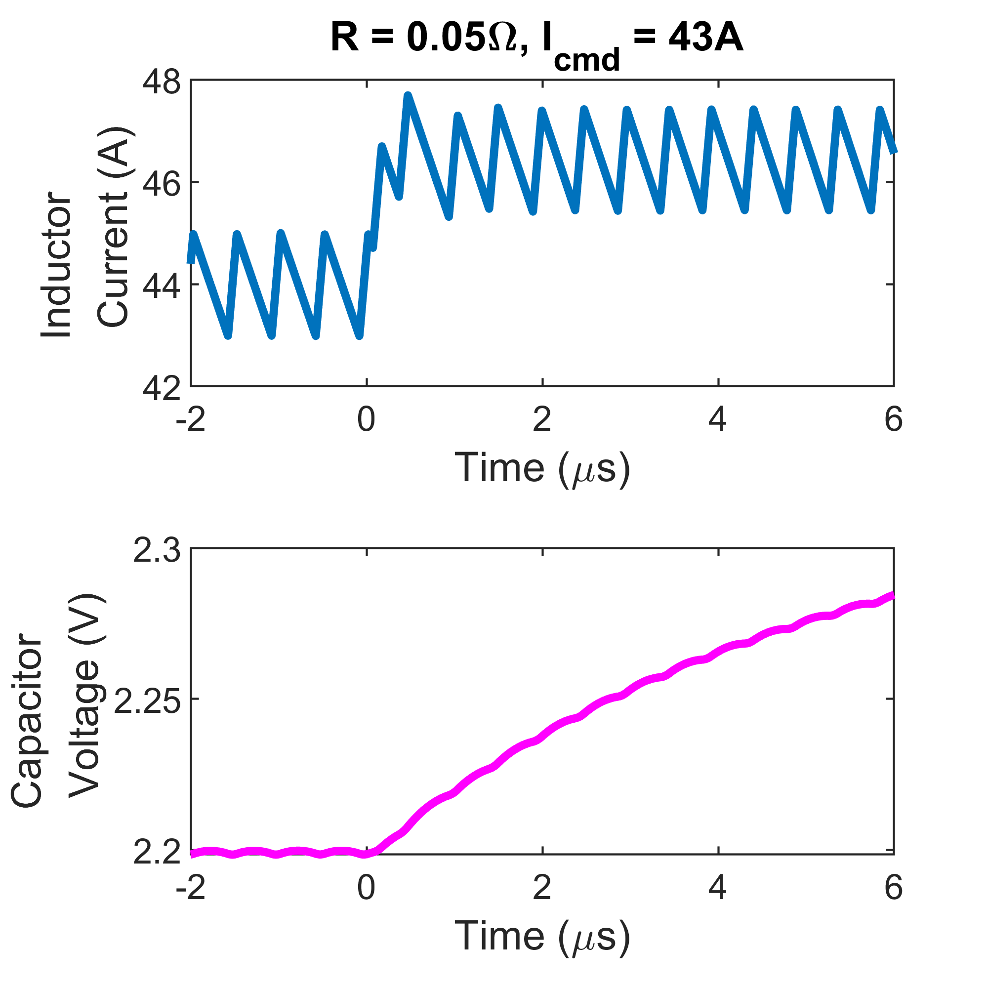
Figure 8: In case study 2, for $R=0.05\,\Omega$ and $I_{\text{cmd}}=43\,\text{A}$, according to the proposed stability criterion (39), the current control loop is stable when the interference is sector-bounded by $|\hat{\alpha}|<0.44$. In the Simulink simulation, the interference with sector bound $|\hat{\alpha}|=0.3$ is added to the inductor current measurement; the inductor current waveform is stable for a current step.

VI Conclusion

The theoretical contribution of this paper provides an analytical and practical stability criterion for designing current-mode dc-dc converters with large-signal stability guarantees. The criteria indicate that the $L/R$ and $RC$ time constants are the design parameters which determine the amount of coupling between the current block and voltage block. The current block and voltage block can be decoupled by increasing $L/R$, $RC$, or $T_{s}^{\text{min}}$, or by decreasing $T_{s}^{\text{max}}$.

References

[1]
F. C. Lee and Q. Li, “High-frequency integrated point-of-load converters:
overview,” IEEE Transactions on Power Electronics, vol. 28, no. 9,
pp. 4127–4136, 2013.
[2]
V. Svikovic, J. J. Cortes, P. Alou, J. A. Oliver, O. Garcia, and J. A. Cobos,
“Multiphase current-controlled buck converter with energy recycling output
impedance correction circuit (OICC),” IEEE Transactions on Power
Electronics, vol. 30, pp. 5207–5222, Sept. 2015.
[3]
M. Yilmaz and P. T. Krein, “Review of battery charger topologies, charging
power levels, and infrastructure for plug-in electric and hybrid vehicles,”
IEEE Transactions on Power Electronics, vol. 28, no. 5, pp. 2151–2169,
2013.
[4]
X. Cui, C. Keller, and A.-T. Avestruz, “Cycle-by-cycle digital control of a
multi-Megahertz variable-frequency boost converter for automatic power
control of LiDAR,” in 2019 IEEE Energy Conversion Congress and
Exposition (ECCE), (Baltimore), pp. 702–711, 2019.
[5]
R. W. Erickson and D. Maksimovic, Fundamentals of Power Electronics.
Springer Science and Business Media, 2007.
[6]
X. Cui and A.-T. Avestruz, “A new framework for cycle-by-cycle digital control
of megahertz-range variable frequency buck converters,” in 2018 IEEE
19th Workshop on Control and Modeling for Power Electronics (COMPEL),
(Padova), pp. 1–8, 2018.
[7]
X. Cui and A.-T. Avestruz, “A 5MHz high-speed saturating inductor dcdc
converter using cycle-by-cycle digital control,” in 2019 IEEE 20th
Workshop on Control and Modeling for Power Electronics (COMPEL), (Toronto),
pp. 1–8, 2019.
[8]
X. Cui and A.-T. Avestruz, “Switching-synchronized sampled-state space
modeling and digital controller for a constant off-time, current-mode boost
converter,” in 2019 American Control Conference (ACC), (Philadelphia),
pp. 1–8, 2019.
[9]
L. Ding, S.-C. Wong, and C. K. Tse, “Bifurcation analysis of a current-mode
controlled dc cascaded system and applications to design,” IEEE Journal
of Emerging and Selected Topics in Power Electronics, vol. 8,
pp. 3214–3224, Dec. 2020.
[10]
R. Redl and I. Novak, “Instabilities in current-mode controlled switching
voltage regulators,” in 1981 IEEE Annual Power Electronics Specialists
Conference, pp. 17–28, 1981.
[11]
X. Cui and A.-T. Avestruz, “Overcoming high frequency limitations of
current-mode control using a control conditioning approach - Part I:
Modeling and analysis,” arXiv:2206.10518, 2022.
[12]
S. Boyd, L. El Ghaoui, E. Feron, and V. Balakrishnan, Linear Matrix
Inequalities in System and Control Theory.
SIAM, 1994.
[13]
Y. Okuyama, Discrete Control Systems.
Springer, Nov. 2014.
[14]
H. K. Khalil, Nonlinear Systems.
Upper Saddle River, 2002.
[15]
X. Cui and A.-T. Avestruz, “Large-signal stability analysis of current-mode
dc-dc converters,” arXiv:2205.10155, pp. 1–8, 2022.