Towards efficient feature sharing in MIMO architectures

Abstract

Multi-input multi-output architectures propose to train multiple subnetworks within one base network and then average the subnetwork predictions to benefit from ensembling for free. Despite some relative success, these architectures are wasteful in their use of parameters. Indeed, we highlight in this paper that the learned subnetwork fail to share even generic features which limits their applicability on smaller mobile and AR/VR devices. We posit this behavior stems from an ill-posed part of the multi-input multi-output framework. To solve this issue, we propose a novel unmixing step in MIMO architectures that allows subnetworks to properly share features. Preliminary experiments on CIFAR 100 show our adjustments allow feature sharing and improve model performance for small architectures.

1 Introduction

The last decade has seen large deep architectures take over many machine learning domains [5, 3] previously solved by more traditional algorithms. As such, deep learning has become ever more present in practical applications. It is therefore now especially important to find ways to maximize model performance [16, 12].

A well known way to obtain better performances given already trained models is to ensemble the predictions given by multiple models [6]. Indeed, predictions from independently trained models have been shown to complement each other such that the aggregated predictions largely outperform the individual model predictions on a test set.

Unfortunately, this increase in performance comes at the cost of dramatically increased overhead : to ensemble multiple models, one must have access to multiple trained models [6, 1]. This is an untenable cost in many real world applications where networks must fit on tiny embedded chips in mobile and AR/VR devices. Significant emphasis has therefore been put in the ensembling literature on finding ways to minimize the inherent cost of ensembling, typically through some degree of parameter sharing between models [7, 13].

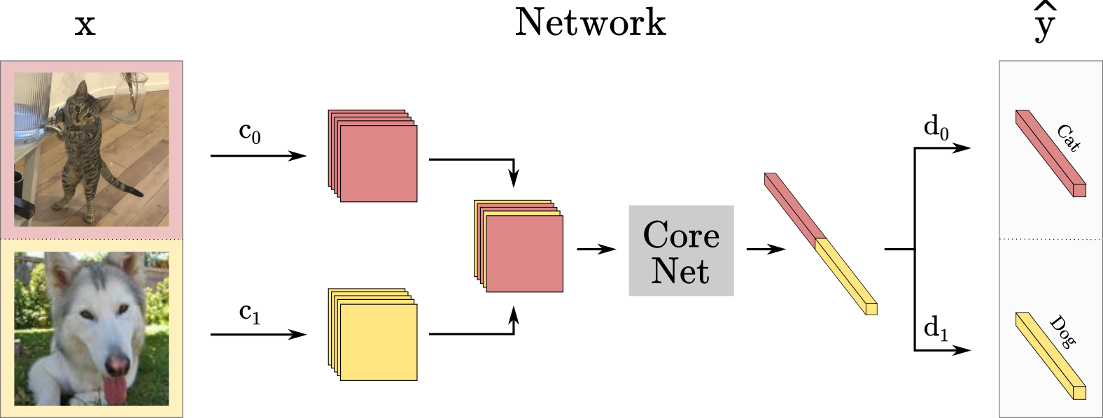
(a) Previous MIMO models train subnetworks that fail to share features.

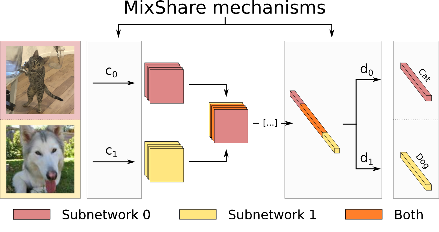
(b) MixShare introduces mechanisms that allow feature sharing.

Figure 1: The lack of feature sharing in MIMO models is a missed opportunity for parameter efficiency on smaller networks. Mixshare introduces unmixing to allow feature sharing among subnetworks in multi-input multi-output models, improving them on smaller networks previous methods struggle on.

Multi-input multi-output (MIMO) strategies [2, 11] provide an interesting solution to this conundrum by ensembling for virtually free. Through their multiple inputs and outputs, MIMO frameworks train independent subnetworks within a base network. Thanks to the sparse nature of large neural networks [8], the resulting subnetworks yield strong and diverse predictions that can be ensembled. As shown on Fig. 1(a) with $M=2$, the $M$ inputs are embedded by $M$ subnetworks with no structural differences. Thus, we have $M$ (inputs, labels) pairs in training: $\{(x_{i},y_{i})\}_{0\leq i<M}$. More precisely, $M$ images are fed to the network at once. The $M$ inputs are encoded by $M$ distinct convolutional layers $\{c_{i}\}_{0\leq i<M}$ into a shared latent space before being aggregated (either through summation [2] or more complex mixing operations [11]). This representation is then processed by the core network into a single feature vector, which is classified by $M$ dense layers $\{d_{i}\}_{0\leq i<M}$. Diverse subnetworks appear as $d_{i}$ learns to classify $y_{i}$ from input $x_{i}$. At inference, we can ensemble $M$ predictions by feeding the same image $M$ times to the model.

MixMo [11] has however recently highlighted significant limitations of such architectures: multi-input multi-output architectures require large base models and struggle to fit more than 2 subnetworks. Indeed, [11] shows a significant drop in performance on CIFAR 100 when going from 2 subnetworks to 4 subnetworks.

This scaling issue is explained by analyzing the features inside the network, as we show at the beginning of this paper by extending [2, 11]’s study of subnetwork behavior. Our analysis shows that the aforementioned scaling issues stem from how subnetworks share no features in the base network (see Fig. 1(a)): each channel or feature is almost exclusively used by one subnetwork. As such, we can explain the scaling issue since each additional subnetwork significantly reduces the effective size of the individual subnetworks. Beyond causing issues on smaller architectures or harder datasets, this leads to very wasteful use of network parameters. This is especially unfortunate as the subnetworks could at the very least share generic features in the first layers. We see this as a missed opportunity, one that can significantly improve multi-input multi-output models’ applicability to real world settings like mobile devices.

In this paper, we first carefully study in Sec. 2 how subnetworks use the base network’s features. After showing the lack of feature sharing, we discuss the impact of this on parameter efficiency and model performance. Secondly, we propose Mixshare in Sec. 3 to address the issues preventing feature sharing (see Fig. 1(b)). In particular, we introduce a novel unmixing mechanism (Sec. 3.1) to allow sharing and discuss in Sec. 3.2 how proper network initialization is necessary to improve model performance.

2 MIMO Subnetworks do not share features

In this section, we strive to pinpoint the cause of multi-input multi-output architectures’ scaling issues. To this end, we consider the following question: how do subnetworks behave in multi-input multi-output architectures ?

Following [11], we check how the inputs are organized in the $C$ feature maps of the mixing space by considering the $L_{1}$ norm of the $C$ encoder kernels for each subnetwork (see Fig. 2). This tells us whether a feature map contains more information about one input, and we can visualize which maps are used by which subnetwork through histograms $h_{0}$ and $h_{1}$ of feature influence for each subnetwork. Quantitatively, we can approximate the feature sharing rate through the ratio of $\frac{\min(h_{0},h_{1})}{\max(h_{0},h_{1})}$. In the same spirit, we consider the $L_{1}$ norm of the columns of classifier weight matrices to quantify the importance of each feature to each classifier.

We conduct our study on a WideResNet-28-2 [15] using the more realistic batch repetition 2 setting from [11] on the CIFAR 100 dataset [4] (see Appendix). We choose to consider this situation as it perfectly showcases the issues encountered by MIMO methods on smaller architectures. To complement this, we also show results on the slightly larger WideResNet-28-5 later on in the paper.

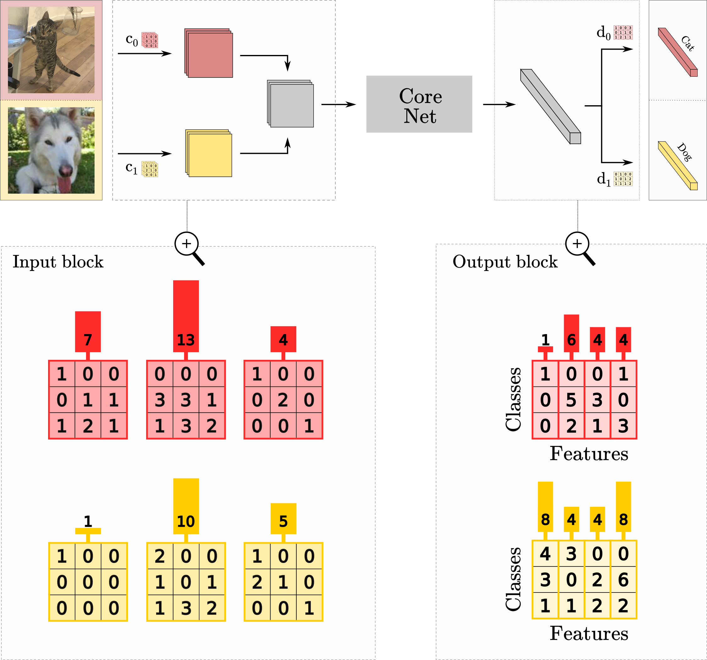
Figure 2: We study the influence of features in the input and output block on the subnetworks ($L_{1}$ norm figured by bars). For the input block, we consider the $L_{1}$ norm of the feature kernels for the relevant encoders. For the output block, we look at the $L_{1}$ norm of columns in the classifier weights matrices. On the figure, this shows us the first input block kernel is mostly used by the first (red) subnetwork (7 vs. 1). Similarly, the first feature of the output block proves important only to the first (red) classifier.

Fig. 3 shows the subnetworks are fully independent in the core network: each channel in the input block encodes information about only one input, as the corresponding kernel of the other encoder’s $L_{1}$ is very low. A similar behavior is observed in the output block, and further analysis of input influence on intermediary feature maps shows this behavior remains consistent within the network (See Appendix).

Multi-input multi-output architectures’ scaling issues become much easier to understand in light of this: the amount of weights available to each of the underlying subnetworks decreases quadratically with the number of subnetwork. Indeed, since feature maps of different subnetworks cannot communicate, only $\frac{1}{M}$ weights can be non-zero. This fraction of non-zero weights must then be distributed between the $M$ subnetworks. Furthermore, the subnetworks likely extract similar generic features, at least in the first layers. Since the subnetworks share no features, this means those features are unnecessarily replicated for each subnetwork.

This is not wholly surprising or undesirable behavior as MIMO strives to train $M$ independent subnetworks to obtain diverse ensembles. By avoiding overlap between subnetworks, the subnetworks act as a standard ensemble of smaller models, with the base model size acting as hard cap on the number of the parameters used by the ensemble.

While it is true not sharing any features ensures subnetworks’ independence, it seems unnecessary. Indeed, the subnetworks are highly unlikely to extract completely different features. As such, subnetworks should benefit from sharing features at least in the early layers even if the classifier still consider fairly different features.

At first blush, nothing in the MIMO training protocol explicitly requires the subnetworks not share any features. Why do the subnetworks avoid sharing features ? How could we encourage them to share some parameters ?

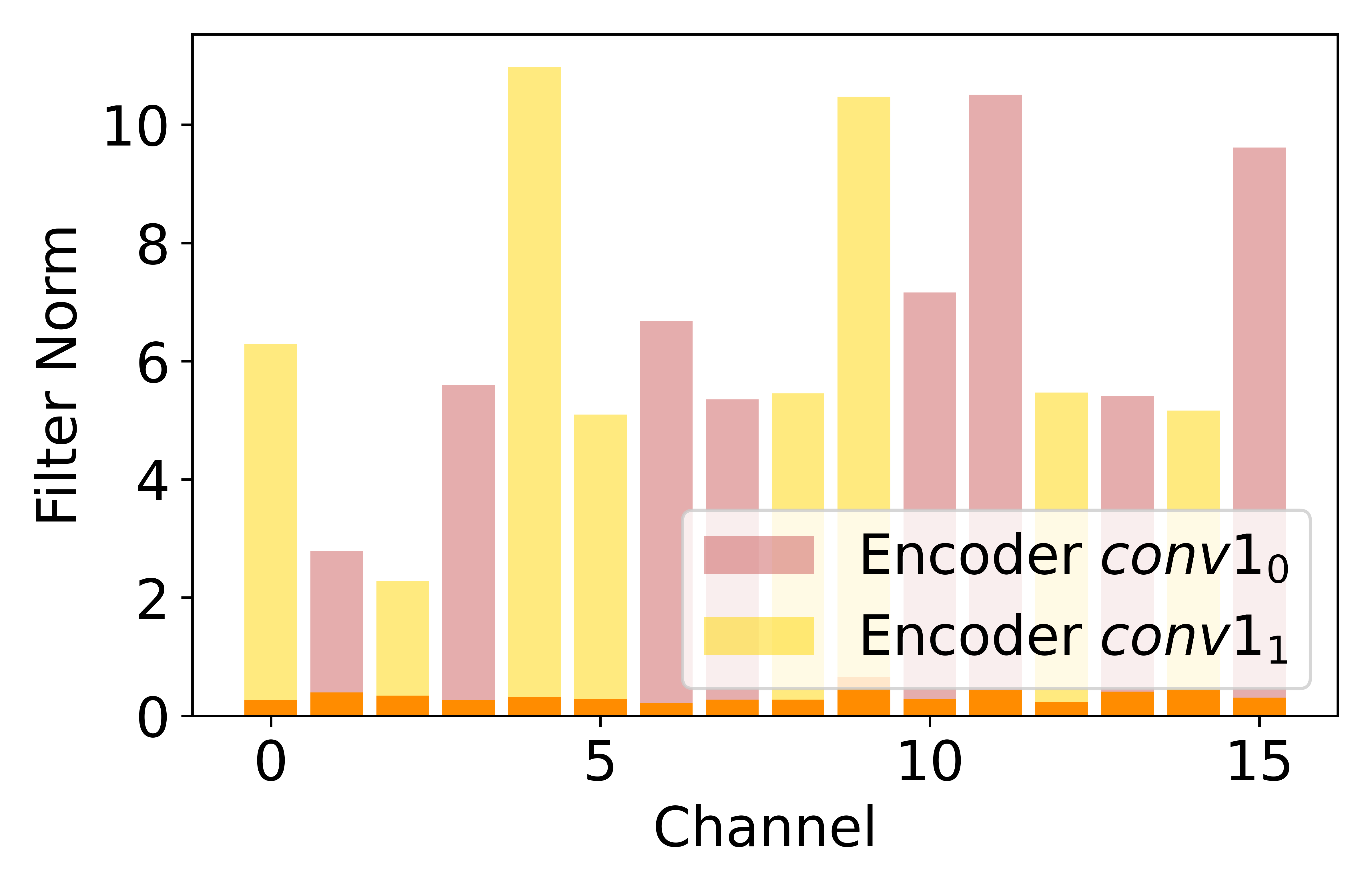
(a) Encoder kernels $L_{1}$ norm.

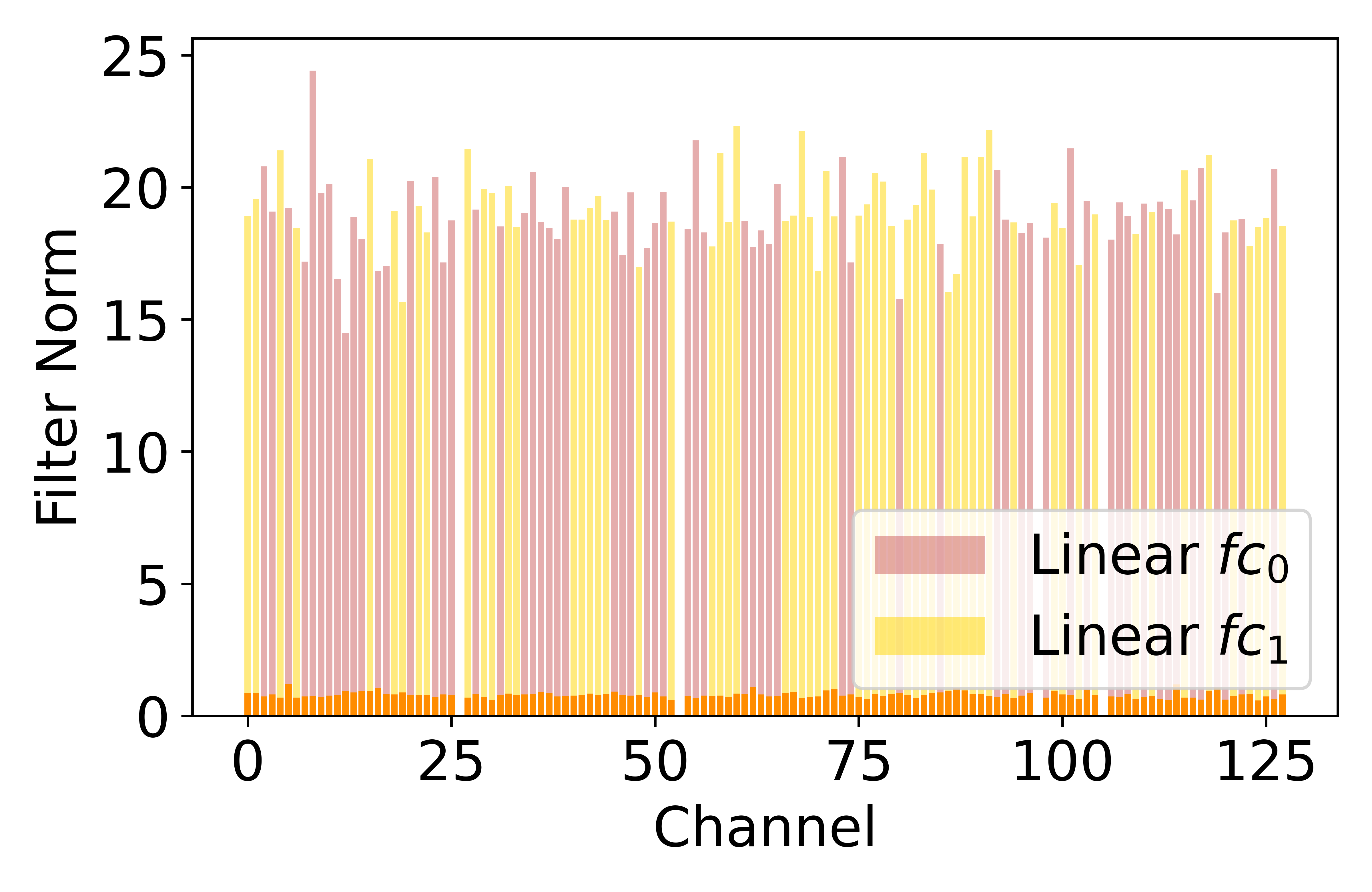
(b) Classifier columns $L_{1}$ norm.

Figure 3: Features are used by one subnetwork or the other, never both at the same time: the overlap (orange) is very low.

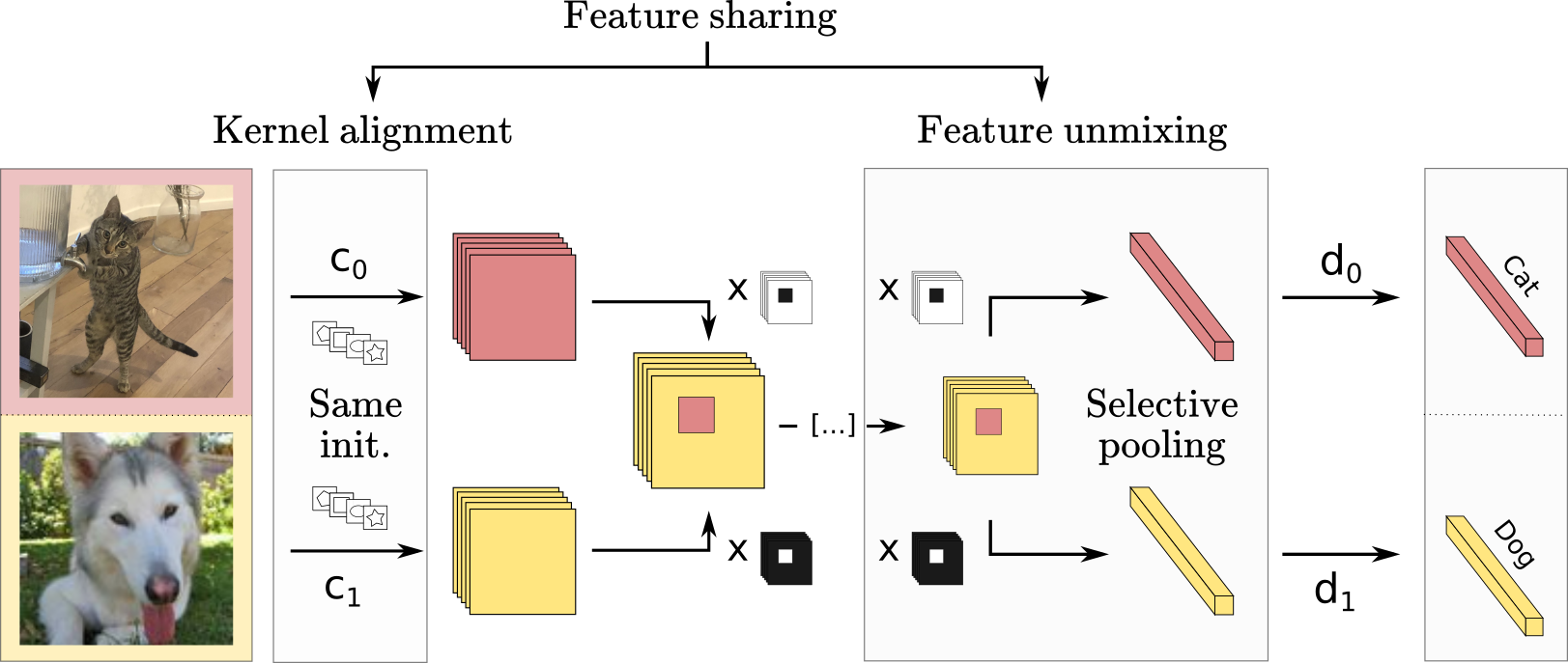
Figure 4: Two steps are necessary to allow feature sharing in networks: 1) Ensure the subnetworks share a “common language” by initializing the convolutional encoders to be close to each other. 2) Extract descriptions of each input from model features.

3 How can subnetworks share features ?

We discuss here the obstacles preventing feature sharing in multi-input multi-output architectures, and propose solutions to correct this behavior.

3.1 Unmixing: extracting features for each input

We build upon an intuition put forth in MixMo [11]: the lack of feature sharing is caused by the need for individual classifier at the end of the network to extract class information for one input specifically. Indeed, the $M$ classifiers have access to the exact same set of extracted features. If two classifiers use the same feature, that feature needs to describe the state of two different inputs. This is an issue when one accounts for the fact inputs are in fact drawn independently and there can therefore be no meaningful feature describing the state of two inputs simultaneously.

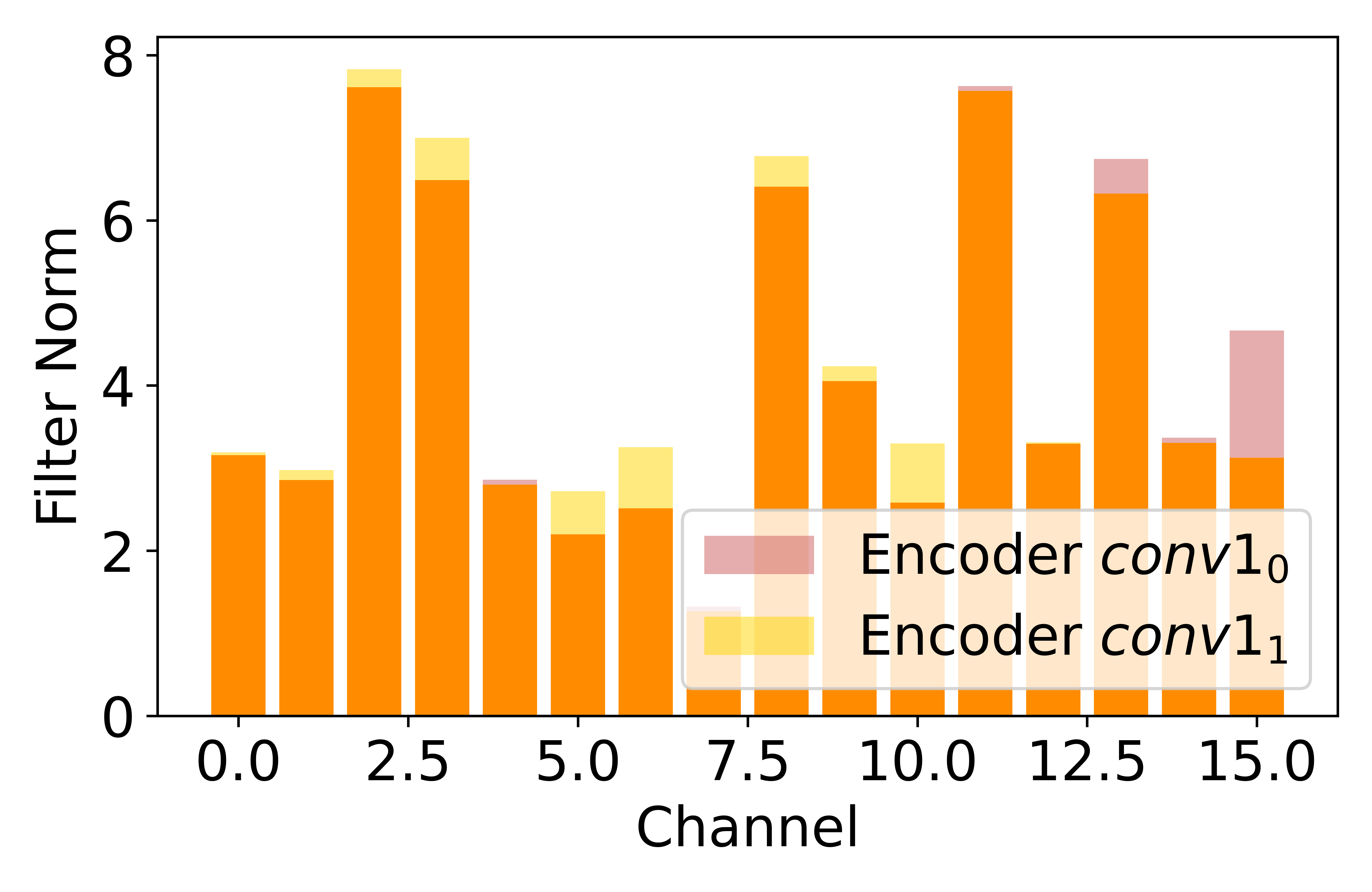
(a) Encoder kernels $L_{1}$ norm.

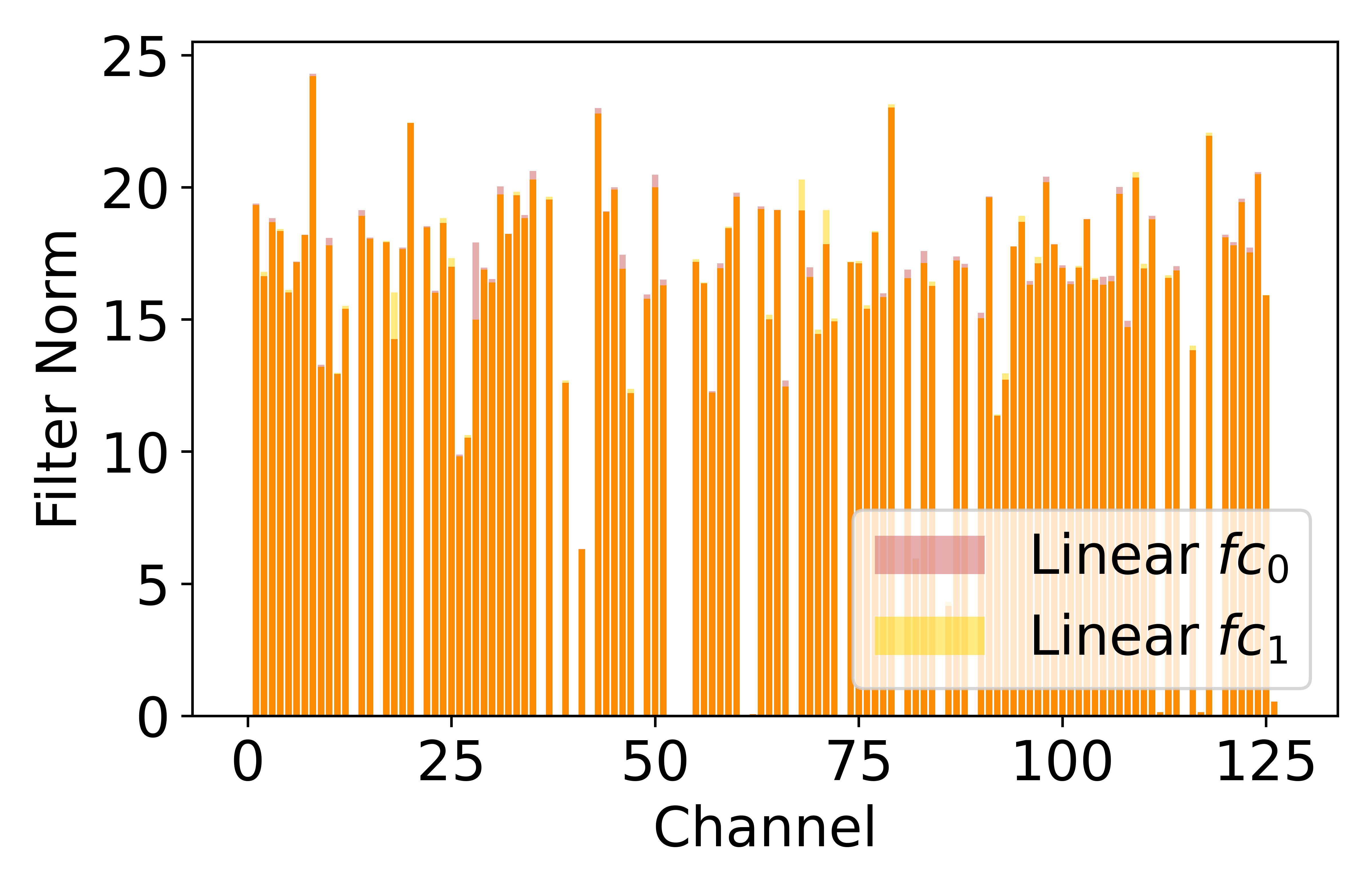
(b) Classifier columns $L_{1}$ norm.

Figure 5: Applying unmixing leads to features being used by both subnetworks: the overlap (orange) is very high.

Method	28-2			28-5
	Acc. ens.	Acc. Ind.	Classifier share rate	Acc. ens.	Acc. Ind.	Classifier share rate
MixMo	$74.8\pm 0.2$	$71.6\pm 0.2$	$4.9\pm 0.4$	$81.9\pm 0.1$	$79.4\pm 0.2$	$8.2\pm 0.1$
MixMo + Unmix	$69.7\pm 15.4$	$69.7\pm 15.4$	$99.1\pm 0.4$	$79.4\pm 2.7$	$79.4\pm 2.7$	$98.8\pm 0.7$
MixMo + Unmix + kernel init.	$\mathbf{79.0\pm 0.1}$	$79.0\pm 0.1$	$99.4\pm 0.1$	$82.1\pm 0.2$	$82.1\pm 0.2$	$99.3\pm 0.1$
MixShare (partial on 25% features)	$73.3\pm 0.5$	$71.5\pm 1.0$	$60.6\pm 6.5$	$79.9\pm 0.3$	$78.8\pm 0.4$	$60.0\pm 2.3$
MixShare (fadeout to 100 epochs)	$\mathbf{79.0\pm 0.1}$	$76.7\pm 1.3$	$64.4\pm 6.0$	$\mathbf{82.4\pm 0.3}$	$81.6\pm 0.5$	$62.7\pm 8.3$

Table 1: Overall ensemble accuracy (%), average subnetwork accuracy (%) and classifier (output block) sharing rate (see Sec. 2) for MixMo variants, $mean\pm std$ reported over 3 runs. Mixshare with fadeout unmixing yields both strong individual models and ensemble gains.

Let us now consider how the classifiers should ideally behave on shared features. Since each classifier is paired to one of the input pathways, they should be able to extract two different interpretations of the shared features that still encode the same functional information (see Fig. 4). For instance, the shared feature should encode for the presence of flowers but each classifier should be able to infer from the feature whether its personal input contains flowers.

While this is not the case in traditional CNNs, MixMo [11] introduces a modification to the seminal MIMO architecture that causes feature maps to encode information about the different inputs separately. Indeed, since MixMo mixes inputs according to some binary mixing augmentation scheme (typically CutMix [14]), each pixel on the final feature maps encodes information about one of the inputs.

This is fortunate as it provides us with a fairly natural solution: unmixing. Unmixing (illustrated in Fig. 4) recycles the binary masks generated for input mixing in order to filter the feature maps so that only information relevant to a specific input is contained in the unmixed version. This way, a single feature map can describe each of the inputs.

Fig. 5 shows that applying unmixing causes the subnetworks to share features, both in the input and output block. In fact, every feature in the unmixed model is used by all subnetworks which proves unmixing indeed solves the core obstacle to feature sharing in MIMO networks.

Introducing unmixing however leads to unstable and generally worse performance as seen in Tab. 1. Crucially, even individual subnetwork accuracy suffers from unmixing which suggests an underlying issue.

3.2 Aligning encoder kernels to allow efficient feature sharing

Intuitively, feature sharing should at the very least lead to higher individual subnetwork accuracy as the subnetworks use more parameters. As such, we now investigate why unmixing degrades performance so dramatically.

By extracting multiple possible interpretations of a single feature, unmixing introduces a new problem in the model. Indeed, we need our interpretations of the same feature to encode the same functional characteristics (e.g. flower detection). The issue is that a randomly initialized multi-input multi-output network typically leads to having multiple interpretations of the same feature.

Indeed, the encoders computing the mixed representations are very different. For an input feature, the mixed feature map could contain information about horizontal borders on input 1 and vertical borders on input 2. As such, there is no consistent interpretation for our mixed features.

We can unify the interpretation of unmixed features at the start by simply aligning the kernels of the encoders. Indeed, as long as each feature encodes the same sort of information for each encoder, there should be no ambiguity introduced by the unmixing process.

Tab. 1 shows that fixing the initialization scheme of the encoders to the same value does indeed lead the model to outperform normal mixmo models.

3.3 Towards partial feature sharing

While proper unmixing does allow feature sharing in multi-input multi-output networks, Tab. 1 and Fig. 5 show it leads to subnetworks sharing all features: the subnetworks are identical. This is even less desirable than fully separated subnetworks as it makes ensembling pointless [9, 10].

Ideally, subnetworks would share some parameters but still remain distinct functionally. This way, we would be able to strike a compromise between fully separated and fully shared subnetworks. The issue with this however, is that removing obstacles to feature sharing makes it unnecessary for subnetworks to separate in any way.

In this preliminary work, we discuss two solutions: partial unmixing and fadeout unmixing. Partial unmixing is a straightforward solution where we only apply unmixing to a fixed subset of the final feature maps (e.g. 25%). In Fadeout unmixing we start training the network with proper unmixing but progressively reduce the strength of unmixing so that there is no unmixing towards the end of the procedure. For instance, we use the unmixing mask $M+r(1-M)$ (instead of $M$) with $r=\min(1,epoch/100)$ if we want to stop unmixing by epoch 100. As such, fadeout unmixing initializes the network in a shared state and progressively pushes the subnetworks to develop independent features.

We now propose the full MixShare framework by combining proper kernel initialization and partial/fadeout unmixing along with slight adjustments to standard MIMO procedures like input repetition [2] and loss balancing [11] (see Appendix). Tab. 1 shows that both MixShare variants succeed in causing partial feature sharing. Partial fails to train strong individual subnetworks, but still showcases ensemble benefits. Fadeout on the other hand leads to strong performances and retains significant ensembling benefits on medium sized networks like a WideResNet 28-5.

4 Conclusion

We have shown multi-input multi-output models induce fully separated subnetworks because of a difficulty in matching outputs to inputs for the neural network. We have proposed an unmixing mechanism and encoder initialization for MixMo [11] architectures and demonstrated it allows multi-input multi-output architectures to share features. Our preliminary experiments show this corrected architecture outperforms standard multi-input multi-output architectures on smaller networks with a proper unmixing scheme. We hope that by highlighting the main issue at the crux of these architectures’ inefficiency, our work will lead to further research on MIMO architectures that will lead to their deployment smaller mobile and AR/VR devices.

Acknowledgments

This work was conducted using HPC resources from GENCI–IDRIS (Grant 2021-AD011013208), and under a CIFRE grant between Thales Land and Air Systems and Sorbonne University.

Appendix

Appendix A Experimental details

The code for this work was directly adapted from the official MixMo [11] codebase: https://github.com/alexrame/mixmo-pytorch.

We followed similar experimental settings on CIFAR 100 as MixMo [11] and present here the adapted setting description:

We used standard architecture WRN-28-$w$, with a focus on $w=2$. We re-use the hyper-parameters configuration from MIMO [2] with batch repetition 2 (bar2). The optimizer is SGD with learning rate of $\frac{0.1}{b}\times\frac{\text{batch-size}}{128}$, batch size $64$, linear warmup over 1 epoch, decay rate 0.1 at steps $\{75,150,225\}$, $l_{2}$ regularization 3e-4. We follow standard MSDA practices [14] and set the maximum number of epochs to $300$. Our experiments ran on a single NVIDIA 12Go-TITAN X Pascal GPU.

All experiments were run three times on three fixed seeds from the same version of the codebase. Qualitative results presented in Fig. 3 and Fig. 5 are obtained by visualizing results for the first set of random seeds. Quantitative results presented in Tab. 1 are given in the form of $mean\pm std$ over the three runs.

Appendix B Complementary adjustments to MIMO procedures in MixShare

MIMO methods use a number of auxiliary procedures to train strong subnetworks. However, as MixShare differs significantly from standard MIMO frameworks, it does not use these frameworks to the same extent.

CutMix probability in the input block

MixMo [11] only uses cutmix mixing in its input block about half the time, using a basic summing operation on the two encoded inputs the rest of the time. This is because the model will use a summing operation at test time. Therefore, the use of cutmix at training induces an strong train/test gap that needs to be bridged by the use of summing during training.

We cannot afford to use summing half the time as unmixing relies on the use of cutmix in the input block. However, since our two encoders are very similar (due to our kernel alignment), cutmix and summing (or averaging) behave very similarly and the train/test gap is therefore minimal.

Input Repetition

A slight train/test gap still remains however since the model is rarely presented the same image as input to both subnetworks at training time. We solve this by reprising a procedure introduced in the seminal MIMO paper [2]: input repetition. In our case, we ensure 10% of inputs of our batches are made of repetition of the same image during training.

Loss rebalancing

MixMo [11] introduced a re-weighting function of the subnetwork training losses that rescales the mixing ratios used in the inputs block. These ratios are rescaled to be less lopsided (closer to an even 50/50 split) before being applied to their relevant subnetwork losses. This rescaling is necessary as it ensures all parameters receive sufficient training signal.

We however find in our experiments it is more beneficial to do away with this re-balancing and keep the original mixing ratios, which we explain by the large amount of features shared between subnetworks. Since features are shared, we do not need to worry about some features receiving too little training signal.

Appendix C A more nuanced discussion on kernel alignment

While MixShare uses the exact same initialization of the encoder kernels for simplicity, it is interesting to note much weaker versions of kernel alignment are sufficient to obtain similar results.

Indeed, we found in our experiments that initializing the kernels to be simply co-linear is more than enough to ensure proper feature sharing. In fact, this leads to the exact same performance as using the same initialization and the encoder kernels quickly converge to similar values.

This further validates our intuition that MIMO models need a “common language” to benefit from sharing features: all that is required is for encoder kernels to extract the same “type” of features.

Appendix D Analysis of subnetwork features within the core network

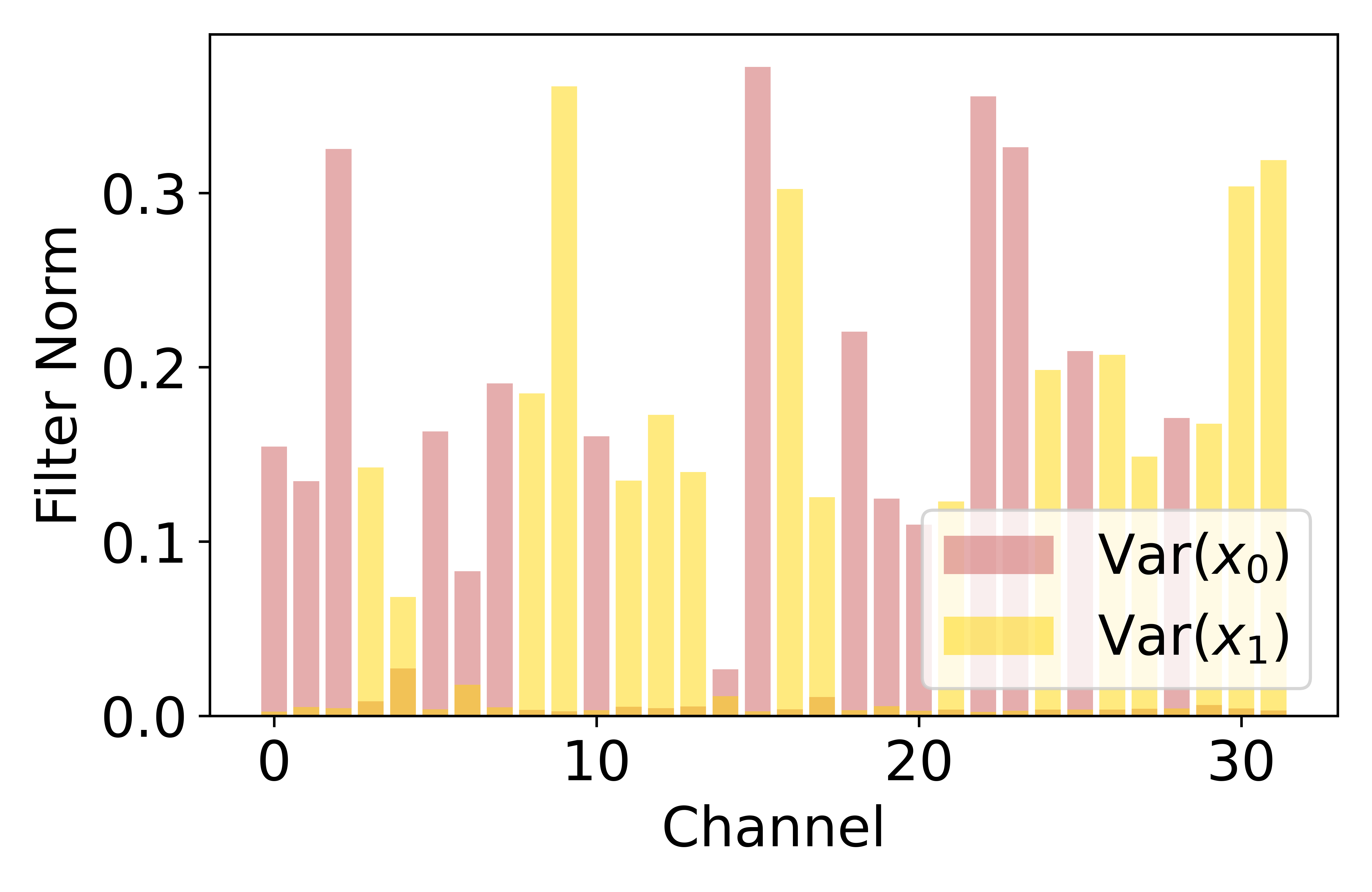
(a) Feature variance after block 1.

(b) Feature variance after block 2.

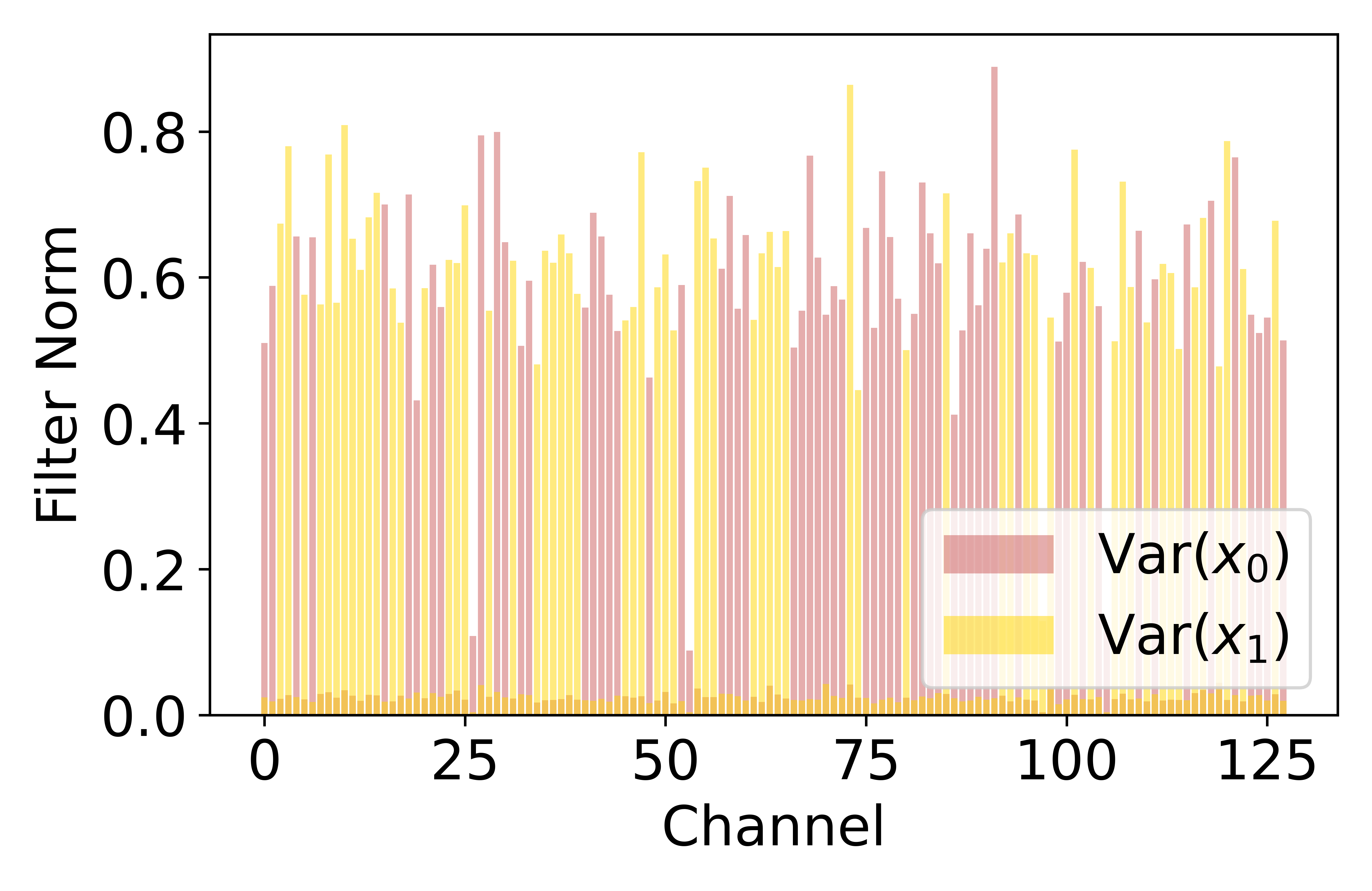
(c) Feature variance after block 3.

Figure 6: Checking the variance of feature maps w.r.t. the two inputs at different levels of the network shows clear separation of features in standard multi-input multi-output architectures.

Sec. 2 studies what features each subnetwork uses in the input block and output block of the multi-input multi-output model. Studying the importance of features within the core networks for each subnetworks is more difficult as it is not possible to consider the model weights. Reprising an analysis conducted in the Appendix of [11], we identify the influence of intermediate features on subnetworks with the variance of the feature with respect to the relevant input.

For the first subnetwork, if we consider the intermediate feature map (at one point in the network $f$) $\mathcal{M}_{int}=f_{int}(\mathcal{D}_{test},d)$, such that $\mathcal{M}_{int}$ is of shape $N\times C\times H\times W$ with $\mathcal{D}_{test}$ the test set, $d$ a fixed input, $N$ the size of the test set, $C$ the number of intermediate feature maps and $H\times W$ the spatial coordinates. We compute the importance of each of the $C$ feature map with respect to the first subnetwork as $Mean(Var(\mathcal{M}_{int},dim=0),dim=(1,2))$. The importance of intermediate features for the second subnetwork is obtained similarly by considering $\mathcal{M}_{int}=f_{int}(d,\mathcal{D}_{test})$.

Fig. 6 shows the resulting feature importance maps at after each of the three residual blocks in the core network. As can be observed, the subnetworks remain consistently separated in the core network.

References

- [1] Lars Kai Hansen and Peter Salamon. Neural network ensembles. IEEE transactions on pattern analysis and machine intelligence, 1990.
- [2] Marton Havasi, Rodolphe Jenatton, Stanislav Fort, Jeremiah Zhe Liu, Jasper Snoek, Balaji Lakshminarayanan, Andrew Mingbo Dai, and Dustin Tran. Training independent subnetworks for robust prediction. In International Conference on Learning Representations, 2021.
- [3] Kaiming He, Xiangyu Zhang, Shaoqing Ren, and Jian Sun. Identity mappings in deep residual networks. In European Conference on Computer Vision, 2016.
- [4] Alex Krizhevsky et al. Learning multiple layers of features from tiny images. 2009.
- [5] Alex Krizhevsky, Ilya Sutskever, and Geoffrey E Hinton. Imagenet classification with deep convolutional neural networks. In Advances in Neural Information Processing Systems, 2012.
- [6] Balaji Lakshminarayanan, Alexander Pritzel, and Charles Blundell. Simple and scalable predictive uncertainty estimation using deep ensembles. In Advances in neural information processing systems, 2017.
- [7] Stefan Lee, Senthil Purushwalkam, Michael Cogswell, David J. Crandall, and Dhruv Batra. Why M heads are better than one: Training a diverse ensemble of deep networks. Arxiv preprint, 2015.
- [8] Eran Malach, Gilad Yehudai, Shai Shalev-Schwartz, and Ohad Shamir. Proving the lottery ticket hypothesis: Pruning is all you need. In International Conference on Machine Learning, 2020.
- [9] Tianyu Pang, Kun Xu, Chao Du, Ning Chen, and Jun Zhu. Improving adversarial robustness via promoting ensemble diversity. In International Conference on Machine Learning, 2019.
- [10] Alexandre Rame and Matthieu Cord. Dice: Diversity in deep ensembles via conditional redundancy adversarial estimation. In International Conference on Learning Representations, 2021.
- [11] Alexandre Rame, Remy Sun, and Matthieu Cord. Mixmo: Mixing multiple inputs for multiple outputs via deep subnetworks. In International Conference on Computer Vision, 2021.
- [12] Divya Shanmugam, Davis Blalock, Guha Balakrishnan, and John Guttag. Better aggregation in test-time augmentation. In International Conference on Computer Vision, 2021.
- [13] Yeming Wen, Dustin Tran, and Jimmy Ba. Batchensemble: an alternative approach to efficient ensemble and lifelong learning. In International Conference on Learning Representations, 2019.
- [14] Sangdoo Yun, Dongyoon Han, Seong Joon Oh, Sanghyuk Chun, Junsuk Choe, and Youngjoon Yoo. Cutmix: Regularization strategy to train strong classifiers with localizable features. In International Conference on Computer Vision, 2019.
- [15] Sergey Zagoruyko and Nikos Komodakis. Wide residual networks. In British Machine Vision Conference, 2016.
- [16] Hongyi Zhang, Moustapha Cisse, Yann N Dauphin, and David Lopez-Paz. mixup: Beyond empirical risk minimization. In International Conference on Learning Representations, 2018.