Stochastic resonance neurons in artificial neural networks

Abstract

We propose a new type of artificial neural networks using stochastic resonance as a dynamic nonlinear node. New design enables significant reduction of the required number of neurons for a given performance accuracy. We also observe that such system is more robust against the impact of noise compared to the conventional analogue neural networks.

Artificial neural networks (ANNs) are capable of solving certain problems using only the accessible sets of training examples, without knowledge of the underlying systems responsible for the generation of this data (see e.g. Goodfellow et al. (2016); LeCun et al. (2015); Brownlee (2018) and references therein). In scientific and engineering applications ANNs can be employed as a non-linear statistical tool that learns low-dimensional representations from complex data and uses this to model nontrivial relationships between inputs and outputs.

Ability of ANNs to predict and approximate from given data is linked to the effective dimensionality - the number of independent free parameters in the model. The approximation capability of the ANNs is quantified by the universal approximation theorems (see for details, e.g. Hornik et al. (1989)). Complexity of the ANNs plays a critical role in the trade-off between their performance and accuracy of the predictions on the one side and power consumption and speed of operation on the other. Many modern applications of ANNs requires over-parametrized models in order to ensure optimal performance, which results in high computational complexity and corresponding increased power consumption.

Power efficiency can be improved using physically implemented (not necessarily digital) neural networks, for instance, designed from layers of controllable physical elements Karniadakis et al. (2021). Physics-inspired or physics-informed analogue neural networks, capable to combine data processing with the knowledge of the underlying physical systems embedded into their architecture Karniadakis et al. (2021); Wright et al. (2022); Li et al. (2016); Kutz and Brunton (2022); Pagnier and Chertkov (2021) is a fascinating area of research offering, in particular, a potential pathway to power-efficient ANNs. There is, however, an essential trade-off between improvements in energy efficiency and susceptibility to noise in the analogue networks. The fundamental challenge in non-digital systems is the accumulation of noise originating from analogue components Drăghici (2000); Semenova et al. (2019); Zhou et al. (2020a); Semenova et al. (2022). To overcome this challenge and unlock full potential of analogue ANNs, it is required to develop systems with capability of absorbing, converting and transforming noise. In this Letter we propose a new design of artificial neural network with stochastic resonance Gammaitoni et al. (1998) used as a network node - ANN-SR.

The robustness of the ANNs operation in the presence of noise depends on the properties of the nonlinear activation function Semenova et al. (2022). Instead of using a conventional static nonlinear element, we employ a dynamical system with bi-stable features (see Fig 1) that can make a positive use of the noise - the stochastic resonance (SR). Note that there are various experimental implementations of SRs that pave the way to new interesting physically implementable designs of ANNs Dodda et al. (2020); Singh et al. (2001). We demonstrate that ANN-SR can significantly reduce the computational complexity and the required number of neurons for a given prediction accuracy. Moreover, ANN-SR performance is more robust against noise in the case of training on noisy data.

Figure 1: Scheme of the considered ESN and the proposed use of dynamic stochastic response functions instead of static ones.

We consider here, as an illustration of our general idea, a particular recurrent neural network schematically shown in Fig. 1, known as echo state network (ESN) Jaeger and Haas (2004), however, the idea of SR neurons can be easily extended to other architectures such as, e.g. deep neural networks. ESNs are fixed recurrent neural networks that constitute a ”reservoir” with multiple (fixed) internal interconnections providing a complex nonlinear multidimensional response to an input signal. An output signal is obtained by training linear combinations only of these read-out ESN responses. The ESN has an internal dynamic memory. The internal connections of the ESN are randomly set up. During the learning procedure the training sequence is fed into the ESN and after an initial transient period the neurons start showing some variations of the fed signal or ”echoing” it. After feeding the training sequence to the ESN the readout weights are calculated.

To explain mathematics behind our idea, we consider the classical ESN model Jaeger and Haas (2004):

$$x_{n+1}=f(\mathbf{W}_{in}u_{n+1}+\mathbf{W}x_{n}+\mathbf{W}_{back}y_{n+1})$$ (1)

where $u\in\mathbb{R}^{M}$ is the current state of the ESN’s input neuron, $x_{n}\in\mathbb{R}^{N\times 1}$ is the vector with dimension $N$ corresponding to the network internal state, matrix $\mathbf{W}^{in}\in\mathbb{R}^{N\times 1}$ is the map of the input $u$ to the vector of dimension $N$, matrix $\mathbf{W}\in\mathbb{R}^{N\times N}$ is the map of the previous state of the recurrent layer, and $f(x)$ is the nonlinear activation function. The recurrent layer consists of $N$ neurons, and the input information $u$ contains a single element at each instance of time. The linear readout layer $\mathbf{W}_{out}$ is defined as

$$y_{n+1}=\mathbf{W}_{out}x_{n+1}$$ (2)

where vector $W_{out}\in\mathbb{R}^{1\times N}$ maps the internal state of the ESN to a single output.

In the classical approach the nonlinear activation function $f(x)$ is a sigmoid or hyperbolic tangent function Jaeger and Haas (2004). We replace in the model 1 the analytical nonlinear function $f(x)$ with a stochastic ordinary differential equation known as stochastic resonance Harikrishnan and Nithin (2021); Anishchenko et al. (1999). The SR phenomenon has been studied in a wide range of physical systems, such as climate modelling, electronic circuits, neural models, chemical reactions, and photonic systems (see e.g. Gammaitoni et al. (1998); Harmer et al. (2002); Harikrishnan and Nithin (2021); Anishchenko et al. (1999); Soriano et al. (2013)). This type of dynamics can be represented using a bi-stable system with two inputs: a coherent signal and a noise Balakrishnan et al. (2019); Harmer et al. (2002). A standard example of the SR model reads:

$$\frac{d\xi(t)}{dt}=-\frac{dU_{0}(\xi)}{d\xi}+s(t)+D\sigma(t).$$ (3)

Here $s(t)$ represents the input signal that will be transformed by the dynamical system into the output signal $\xi(t)$, $\sigma(t)$ is the Gaussian noise with zero mean and variance of 1, where $D$ is the noise amplitude. The stationary potential function $U_{0}$ together with the time-dependent input signal $s(t)$ define the time-dependent landscape of internal evolution of the dynamical system and form the time-dependent tilted potential $U(\xi,t):$

$$U(\xi,t)=U_{0}(\xi)+\xi s(t)$$ (4)

Let us consider a symmetric bi-stable stationary potential well $U_{0}$:

$$U_{0}(x)=-\alpha\cdot\frac{x^{2}}{2}+\beta\cdot\frac{x^{4}}{4}$$ (5)

This model is a limit of the heavily dumped harmonic oscillator, which represents the movement of a particle in the time-dependent bi-stable potential $U(x,t)=U_{0}(x)-xs(t)$ Harmer et al. (2002); Mingesz et al. (2006). When $\alpha>0$, the potential is bi-stable with two stationary points $x_{s}=\pm\sqrt{\alpha/\beta}$ and a barrier of value $\Delta U=\alpha^{2}/(4\beta)$.

Noise is a requisite ingredient in defining SR operation. The utilization of noise as a tool for improving the performance of deep learning algorithms has been widely investigated Nagabushan et al. (2016); Bishop et al. (1995). Noise has been used to combat adversarial attacks Zheltonozhskii et al. (2020); He et al. (2019), as a regularization technique Li and Liu (2016) and as a way to increase the noise robustness of ANNs that are implemented in analogue hardware Zhou et al. (2020b, a). Furthermore, different noise injection techniques and different scenarios with adding noise to the input, weights or activation function are explored in recent studies He et al. (2019); Zhou et al. (2020b). Noise increases the dimensions of the latent feature space Poole et al. (2014); Hayakawa et al. (1995) and the probability of a more chaotic operation. Here we demonstrate that under certain conditions the SR function is superior compared to the classical sigmoid node as a nonlinear activation function. We compare the prediction accuracy and computational complexity and show that SR outperforms the classical approach in both of these aspects.

The standard neuron collects a linear combination of incoming values, applies a nonlinear function to it and passes the result further. The proposed SR neuron is different: it has its own internal state $\xi(t)$, which constitutes memory. This internal state together with the incoming signals from other neurons are used to form the output. The SR neuron collects a linear combination of incoming weights $s$ which modifies the potential function $U$. Then Eq. (3) is integrated on some time interval $\Delta t$ to obtain the next internal state of the SR neuron. This new internal state $\xi(t+\Delta t)$ is the output value of SR neuron.

To evaluate the performance of the SR as the nonlinear function we used a classical problem of predicting the Mackey-Glass (MG) series $q(t)$ (see Supplementary materials). For training and testing the described approach, in addition to the MG series we used a noisy version of the MG series. A part of the MG series is used to train the ESN and the next several tens of points of the MG series are compared to the output of the freely running ESN to estimate the prediction accuracy. During the training and testing, the nonlinear response of each SR neuron is calculated as a result of the integration of Eq. (3) with weighted sum of input neurons as the variable $s$ in Eq. (3) and previous internal state of the neuron as initial condition. As the training and test sequences are parts of the MG series they are time-dependent, therefore, we integrate Eq. (3) over time with $s$ as a parameter. The integration interval $\Delta t$ is equal to the time step of the MG series and we set the initial value of the SR function as $\xi(t=0)=\mathcal{N}(0,1)$. On each time step we take the current value of the function $\xi_{n}$ and calculate the next value by integrating Eq. (3) with $\xi_{n}$ as an initial value:

$$f(s_{n})\equiv\xi_{n+1}\!=\!\xi_{n}\!+\!\left[\alpha(\xi\!-\!\xi^{3})\!+\!D\sigma(t)\right]\!\cdot\Delta t+s_{n}\cdot\Delta t$$ (6)

This is done whenever we need to calculate the nonlinear response function $f(s)$ using a 2nd order Runge-Kutta (RK2) also known as the Euler method.

The output of the nonlinear response function is calculated as a trajectory of a system described by the SR equation with input values as an external force applied to the system. The internal state of the SR system is described by a vector $\xi$ that evolves with time. For a given initial state $\xi_{n}$ and input value $s_{n}$, the output of the SR nonlinear function can be calculated as the next internal state $\xi_{n+1}$ separated from the previous state by time $\Delta t$. Note that there are two sources of noise: (i) implementation noise coming from the active nature of the nonlinear node, and (ii) the noisy data, both practically important and considered in this work.

In the current work we use the proposed approach to design an ESN and estimate its accuracy depending on the number of neurons and noise amplitude in the training data. We compare the designed ESN-SR with the classical ESN with sigmoid activation function in terms of accuracy and computational complexity.

We estimated the computational complexity of ESNs as the number of multiplications needed to perform a single evolutionary step described by Eq. (1) and Eq. (2).

The total numbers of multiplications for 1 step of calculating evolution of the ESN are:

$$Q_{\text{total}}^{\text{classical}}=N^{2}+3N$$ (7)

$$Q_{\text{total}}^{SR}=N^{2}+4N$$

Note that the number of additional multiplications grows linearly with the size of the ESN, the total number of multiplications grows quadratically and $N>>1$, so the quadratic term dominates in the complexity. We used the classical training procedure as described in Jaeger and Haas (2004). This procedure together with the regularization aspects are given in Supplementary materials.

The prediction accuracy is measured by the mean squared error between freely running ESN and corresponding 100 samples of the MG series. Parameters of the ESN under test are as below:

• $N=50\cdots 1000$

• Connectivity of $\mathbf{W}$ is 0.01

• Hyperparameter of the SR function $\alpha=0.01$

• SR noise amplitude $D=0,10^{-10},10^{-8},10^{-6}$

The result of this test is shown in Fig. 2 where each point represents a mean value averaged over 1000 samples.

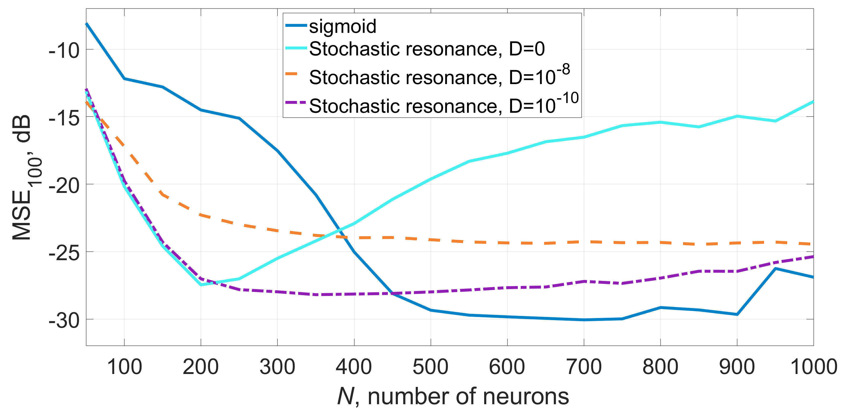
Figure 2: Mean squared error (MSE) for different nonlinear activation functions depending on the number of neurons.

The ”classical” ESN with sigmoid activation function is trained under similar conditions. The linear regression problem for determining the readout weights was performed using singular value matrix decomposition. Other aspects of the training procedure and regularization are given in Supplementary material.

The transfer functions of an SR neuron depends on the number of the ESN evolution step. The initial values (step 1) are normally distributed with mean 0 and variance 1. The transfer function for steps 1, 10, 1000 and 3100 are shown in Fig. 3. Each neuron automatically converges into its own transfer function during the learning procedure, providing a possibility of the self-adjusting activation functions in different layers of ESN using the same design of the node.

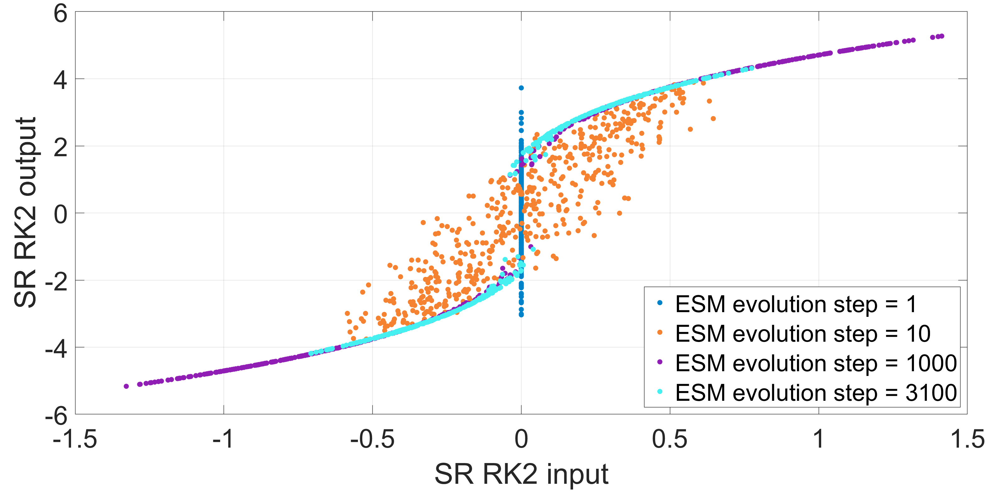
Figure 3: Stochastic resonance transfer function

One can see that for lower number of neurons the performance of ESN-SR is better than the classical approach with a sigmoid activation function. In particular, the SR method reaches its maximum accuracy at $N=200$ neurons with an averaged error of $10^{-2.76}$. The number of multiplications per 1 step is $Q_{\text{total}}^{SR}(N=200)=40800$. For the classical sigmoid an error of $10^{-1.45}$ or 0.036 is achieved for a similar number of nodes $Q_{\text{total}}^{\text{classical}}(N=200)=40600$. So we obtain 20 times more accurate results by using the ESN of same computational complexity. To achieve the same accuracy using the sigmoid activation function one needs to take $N=450$ neurons leading to $Q_{\text{total}}^{\text{classical}}(N=450)=203850$ multiplications per 1 step. So, to achieve the same accuracy using the classical sigmoid function one needs to perform 5 times more multiplications and 2.5 times more nodes. We investigated how the noise amplitude $D$ affects the accuracy and stability of the ESN, see Figs 2 and 4. One can see that the low level of added noise improves the maximum accuracy slightly and also increases stability and accuracy at a higher number of neurons by preventing overfitting. But even slightly higher noise amplitude reduces the accuracy. We also investigated the capability of predicting the continuation of the MG series when learning on noisy sequence. The training sequence was corrupted by white Gaussian noise and fed into the ESN with the same learning procedure as before.
The dependence of the MSE (colour-coded) on number of neurons, internal noise in the nonlinear activation function and SNR of the teaching sequence is shown in Fig. 4 showing the optimal internal SR noise level close to $10^{-10}$.

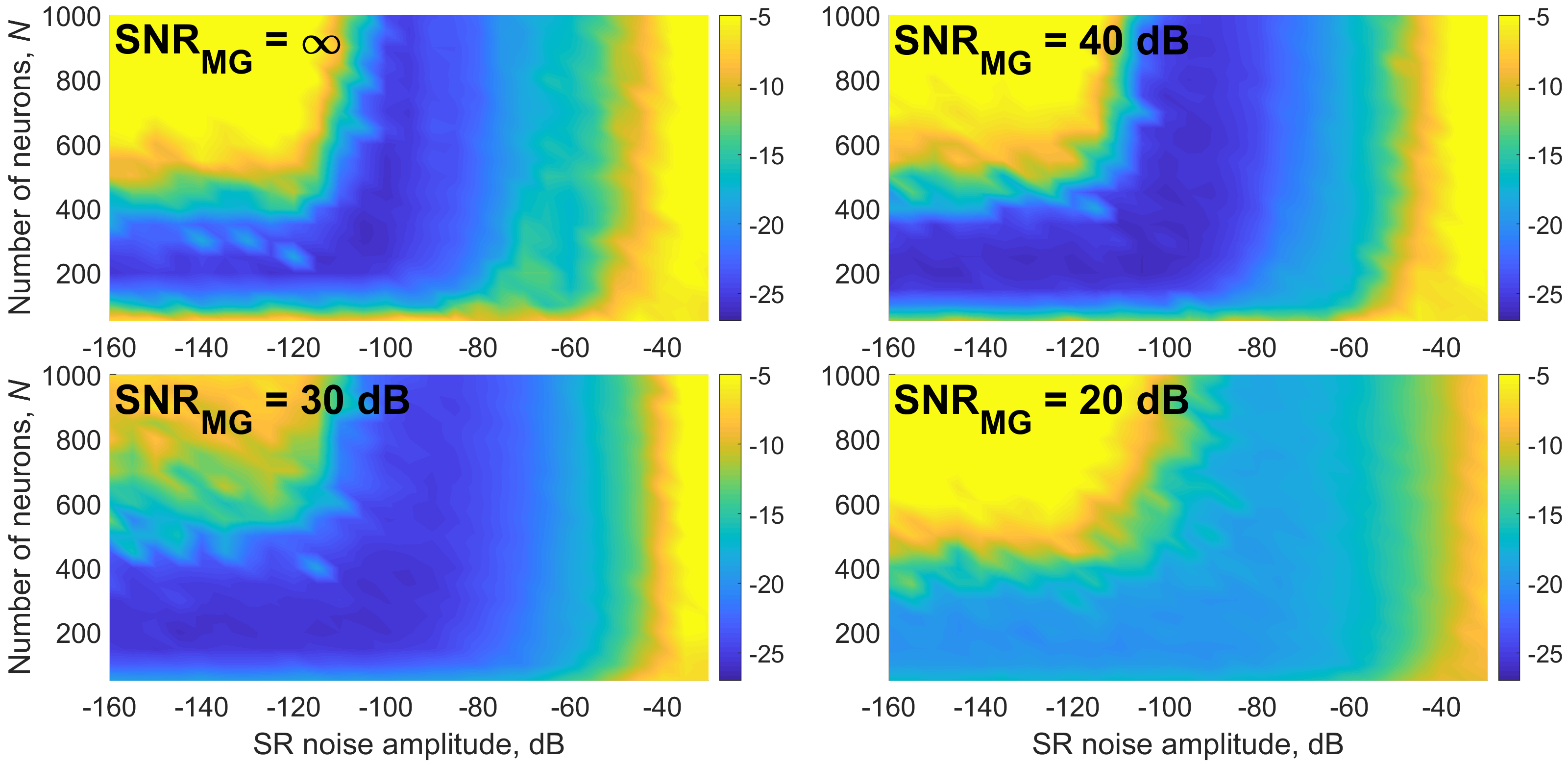
Figure 4: Prediction accuracy (colour-coded) depending on SR noise level, number of neurons and noise in the teaching sequence.

We used the SR function with $D=10^{-10}$ and compared it with classical sigmoid function. Noise amplitudes in the training sequence $\sigma$ corresponding to SNR of $20$, $30$ and $40$ dB were chosen. Figure 5 shows how the MSE of the first 100 predicted values depends on the number of neurons for different nonlinear activation functions and various noise levels in the training sequence.

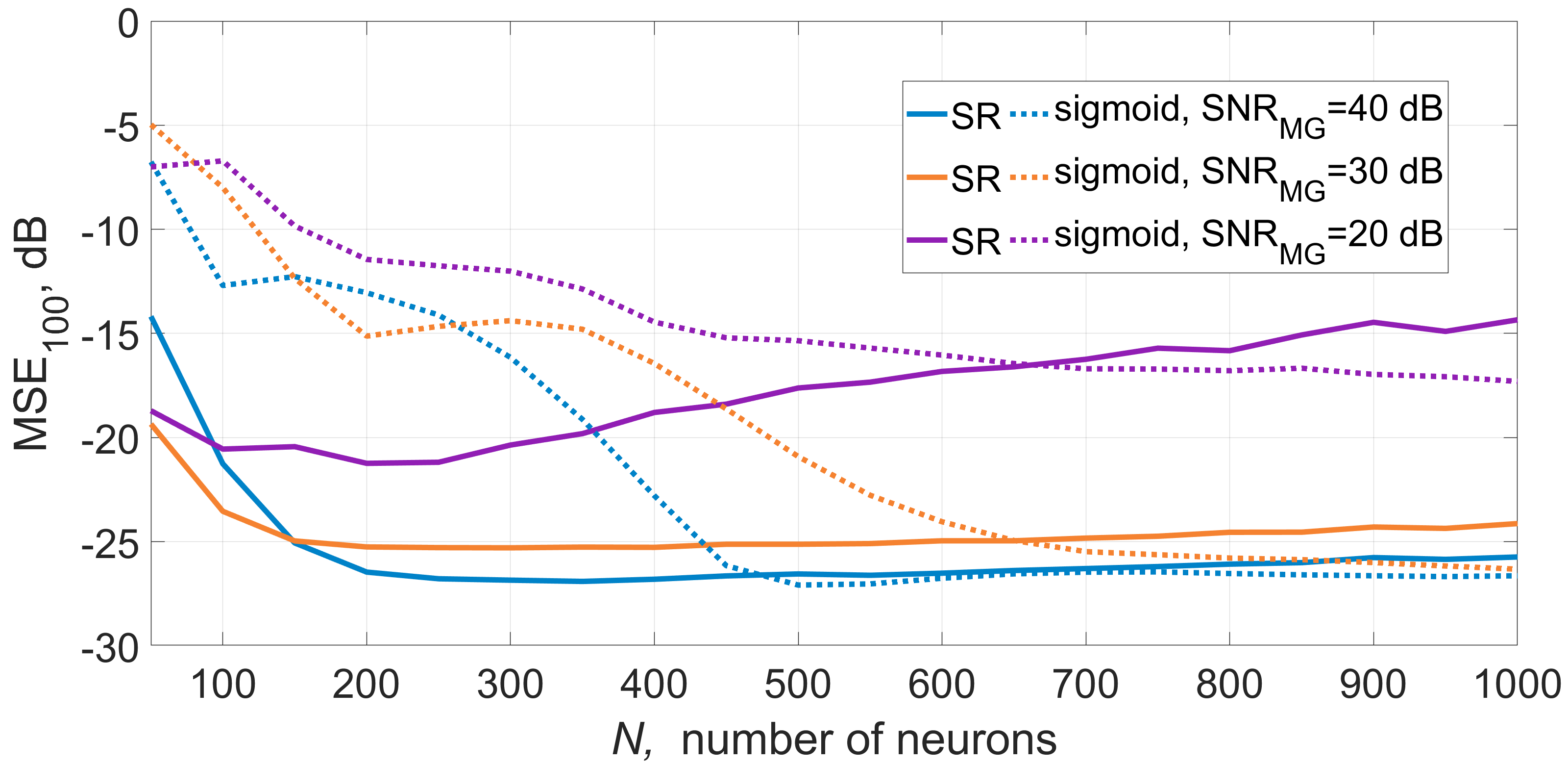
Figure 5: Accuracy of the RC when learning on noisy MG sequence.

The proposed method shows superior performance compared to classical approach in case of lower number of neurons and the same performance for higher number of neurons. In particular, is case of SNR $=20$ dB the prediction accuracy is as good as $0.01$ when the number of neurons is as low as $100$ in case of SR. The use of sigmoid function provides 24 times less accurate results at this number of neurons. And this accuracy is never achieved with the classical sigmoid function even at higher number of neurons at this level of noise in the training sequence. Figure 6 shows how the best prediction accuracy across various number of neurons depends on the SNR in the training sequence where shaded regions depict one standard deviation intervals calculated on 1000 runs.

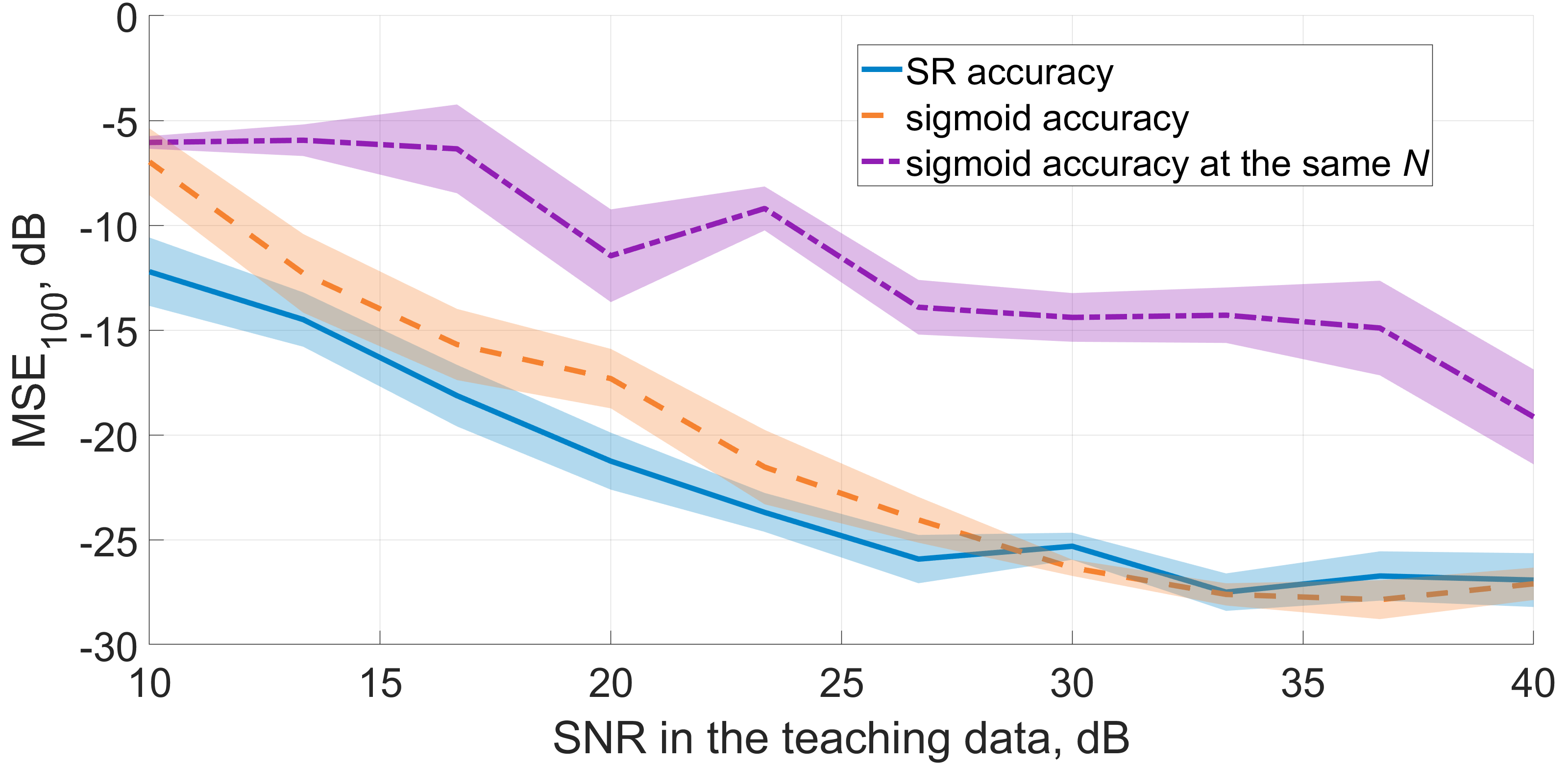
Figure 6: Best accuracy across ESNs of various complexity. Shaded areas depict one standard deviation intervals.

As can be seen in Fig. 6 while there is no statistically significant difference between the performance of the ESN-SR and sigmoid system for SNR $>25$ dB, the latter outperforms the former in other regions especially when the number of nodes is the same (violet curve). We believe this result is particularly important for training on experimental data as it is always corrupted by noise.
In this work we proposed using SR as a nonlinear activation function in neural networks and investigated how SR nodes can improve the performance of an ESN. Using standard Mackey-Glass equation benchmark and ESN as an illustration of the general concept, we demonstrated the superiority of an ESN-SR computer to ESN-sigmoid in the case of noisy input data and implementation noise. We showed that our proposed ESN can provide up to 9.5 times better accuracy in predicting the MG time series compared to the conventional ESN with the same number of nodes. This indicates the capability of SR nodes to capture the underlying relations between samples of the input and manifesting memory properties in various ANNs. We believe that the proposed idea of using model (or, indeed, physical systems) governed by stochastic ordinary differential equations can be applied in a range of ANNs and can be generalized to different tasks. In particular, the proposed concept is compatible with high-bandwidth optical analogue ANNs and reservoirs offering potential solutions for high-speed parallel signal processing and reduction in the power consumption in physical implementations.

This work was supported by the EU ITN project POST-DIGITAL and the EPSRC project TRANSNET.

References

- Goodfellow et al. (2016) I. Goodfellow, Y. Bengio, and A. Courville, Deep Learning (MIT Press, 2016) http://www.deeplearningbook.org.
- LeCun et al. (2015) Y. LeCun, Y. Bengio, and G. Hinton, Nature 521, 436 (2015).
- Brownlee (2018) J. Brownlee, Machine Learning Mastery With Python 1 (2018).
- Hornik et al. (1989) K. Hornik, M. Tinchcombe, and H. White, Multilayer Feedforward Networks are Universal Approximators, Neural Networks. Vol. 2., pp. 359–366 (Pergamon Press, 1989).
- Karniadakis et al. (2021) G. E. Karniadakis, I. G. Kevrekidis, L. Lu, P. Perdikaris, S. Wang, and L. Yang, Nature Reviews Physics 3, 422 (2021).
- Wright et al. (2022) L. G. Wright, T. Onodera, M. M. Stein, T. Wang, Z. H. Darren T. Schachter, and P. L. McMahon, Nature 601, 549 (2022).
- Li et al. (2016) M. Li, O. İrsoy, C. Cardie, and H. G. Xing, IEEE Journal on Exploratory Solid-State Computational Devices and Circuits 2, 44 (2016).
- Kutz and Brunton (2022) J. Kutz and S. Brunton, Nonlinear Dynamics 107(3), 1 (2022).
- Pagnier and Chertkov (2021) L. Pagnier and M. Chertkov, arXiv preprint arXiv:2102.06349 (2021).
- Drăghici (2000) S. Drăghici, International journal of neural systems 10 1, 19 (2000).
- Semenova et al. (2019) N. Semenova, X. Porte, L. Andreoli, M. Jacquot, L. Larger, and D. Brunner, Chaos: An Interdisciplinary Journal of Nonlinear Science 29, 103128 (2019).
- Zhou et al. (2020a) C. Zhou, P. Kadambi, M. Mattina, and P. N. Whatmough, arXiv preprint arXiv:2001.04974 (2020a).
- Semenova et al. (2022) N. Semenova, L. Larger, and D. Brunner, Neural Networks 146, 151 (2022).
- Gammaitoni et al. (1998) L. Gammaitoni, P. Hänggi, P. Jung, and F. Marchesoni, Rev. Mod. Phys. 70, 223 (1998).
- Dodda et al. (2020) A. Dodda, A. Oberoi, A. Sebastian, T. H. Choudhury, J. M. Redwing, and S. Das, Nature communications 11, 1 (2020).
- Singh et al. (2001) K. P. Singh, G. Ropars, M. Brunel, F. Bretenaker, and A. Le Floch, Physical Review Letters 87, 213901 (2001).
- Jaeger and Haas (2004) H. Jaeger and H. Haas, Science 304, 78 (2004).
- Harikrishnan and Nithin (2021) N. Harikrishnan and N. Nithin, arXiv preprint arXiv:2102.01316 (2021).
- Anishchenko et al. (1999) V. S. Anishchenko, A. B. Neiman, F. Moss, and L. Shimansky-Geier, Physics-Uspekhi 42, 7 (1999).
- Harmer et al. (2002) G. P. Harmer, B. R. Davis, and D. Abbott, IEEE Transactions on Instrumentation and Measurement 51, 299 (2002).
- Soriano et al. (2013) M. C. Soriano, J. García-Ojalvo, C. R. Mirasso, and I. Fischer, Rev. Mod. Phys. 85, 421 (2013).
- Balakrishnan et al. (2019) H. N. Balakrishnan, A. Kathpalia, S. Saha, and N. Nagaraj, Chaos: An Interdisciplinary Journal of Nonlinear Science 29, 113125 (2019).
- Mingesz et al. (2006) R. Mingesz, Z. Gingl, and P. Makra, Eur. Phys. J. B 50, 339 (2006).
- Nagabushan et al. (2016) N. Nagabushan, N. Satish, and S. Raghuram, in 2016 IEEE International Conference on Computational Intelligence and Computing Research (ICCIC) (IEEE, 2016) pp. 1–5.
- Bishop et al. (1995) C. M. Bishop et al., Neural networks for pattern recognition (Oxford university press, 1995).
- Zheltonozhskii et al. (2020) E. Zheltonozhskii, C. Baskin, Y. Nemcovsky, B. Chmiel, A. Mendelson, and A. M. Bronstein, arXiv preprint arXiv:2003.02188 (2020).
- He et al. (2019) Z. He, A. S. Rakin, and D. Fan, in Proceedings of the IEEE Conference on Computer Vision and Pattern Recognition (2019) pp. 588–597.
- Li and Liu (2016) Y. Li and F. Liu, arXiv preprint arXiv:1612.01490 (2016).
- Zhou et al. (2020b) C. Zhou, P. Kadambi, M. Mattina, and P. N. Whatmough, arXiv preprint arXiv:2001.04974 (2020b).
- Poole et al. (2014) B. Poole, J. Sohl-Dickstein, and S. Ganguli, “Analyzing noise in autoencoders and deep networks,” (2014).
- Hayakawa et al. (1995) Y. Hayakawa, A. Marumoto, and Y. Sawada, Phys. Rev. E 51, R2693 (1995).