Privacy Preserving Image Registration

Abstract

Image registration is a key task in medical imaging applications, allowing to represent medical images in a common spatial reference frame. Current approaches to image registration are generally based on the assumption that the content of the images is usually accessible in clear form, from which the spatial transformation is subsequently estimated. This common assumption may not be met in practical applications, since the sensitive nature of medical images may ultimately require their analysis under privacy constraints, preventing to openly share the image content. In this work, we formulate the problem of image registration under a privacy preserving regime, where images are assumed to be confidential and cannot be disclosed in clear. We derive our privacy preserving image registration framework by extending classical registration paradigms to account for advanced cryptographic tools, such as secure multi-party computation and homomorphic encryption, that enable the execution of operations without leaking the underlying data. To overcome the problem of performance and scalability of cryptographic tools in high dimensions, we propose several techniques to optimize the image registration operations by using gradient approximations, and by revisiting the use of homomorphic encryption trough packing, to allow the efficient encryption and multiplication of large matrices. We demonstrate our privacy preserving framework in linear and non-linear registration problems, evaluating its accuracy and scalability with respect to standard, non-private counterparts. Our results show that privacy preserving image registration is feasible and can be adopted in sensitive medical imaging applications.

1 Introduction

Image Registration is a crucial task in medical imaging applications, allowing to spatially align imaging features between two or multiple scans. Registration methods are today a central component of state-of-the-art methods for atlas-based segmentation [28, 6], morphological and functional analysis [8, 1], multi-modal data integration [15], and longitudinal analysis [23, 2]. Typical registration paradigms are based on a given transformation model (e.g. affine or non-linear), a cost function and an associated optimization routine. A large number of image registration approaches have been proposed in the literature over the last decades, covering a variety of assumptions on the spatial transformations, cost functions, image dimensionality and optimization strategy [27]. Image registration is the workhorse of many real-life medical imaging software and applications, including public web-based services for automated segmentation and labelling of medical images. Using these services generally requires uploading and exchanging medical images over the Internet, to subsequently perform image registration with respect to one or multiple (potentially proprietary) atlases. There are also emerging data analysis paradigms, such as Federated Learning (FL) [19], where medical images can be jointly registered and analysed in multi-centric scenarios to perform group analysis [13]. In these settings, the creation of registration-based image templates [1] is currently not possible without disclosing the image information. For this reason, due to the evolving juridical landscape on data protection, these applications of image registration may not be compliant anymore with regulations currently existing in many countries, such as the European General Data Protection Regulation (GDPR) , or the US Health Insurance Portability and Accountability Act (HIPAA). Medical imaging information falls within the realm of personal health data [17] and its sensitive nature should ultimately require the analysis under privacy preserving constraints, for instance by preventing to share the image content in clear form.

Advanced cryptographic tools enabling data processing without disclosing it in cleartext hold great potential in sensitive data analysis problems (e.g., [16]). Examples of such approaches are Secure-Multi-Party-Computation (MPC) [30] and Homomorphic Encryption (HE) [24]. While MPC allows multiple parties to jointly compute a common function over their private inputs and discover no more than the output of this function, HE enables computation on encrypted data without disclosing either the input data or the result of the computation.

This work presents a new methodological framework allowing image registration under privacy constraints. To this end, we reformulate the image registration problem to integrate cryptographic tools, namely MPC or FHE, thus preserving the privacy of the image data. Due to the well-known scalability issues of such cryptographic techniques, we investigate strategies for the practical use of privacy-preserving image registration (PPIR) through gradient approximations, array packing and matrix partitioning. In our experiments, we evaluate the effectiveness of PPIR in linear and non-linear registration problems. Our results demonstrate the feasibility of PPIR and pave the way for the application of image registration in sensitive medical imaging applications.

2 Background

1:

2:$\triangleright$ Moving image $I$

3:$\triangleright$ Template image $J$

4:$\triangleright$ Distance function $f$

5:$\triangleright$ Spatial transformation ${\bm{W}}_{\bm{\theta}}$, parameterized by ${\bm{\theta}}$

6:$\triangleright$ convergence threshold $\epsilon$

7:

8:$\triangleright$ Transformed image $I({\bm{W}}_{\bm{\theta}})$ after convergence is reached

9:

10:function ImageRegistration($I,J,{\bm{W}}_{\bm{\theta}}$):

11:    ${\bm{\theta}}\longleftarrow$ InitializeParameters()

12:    repeat

13:         $e\longleftarrow$ $f\big{[}I({\bm{W}}_{\bm{\theta}}),J\big{]}$

14:         $G\longleftarrow$ $\frac{\partial f}{\partial{\bm{\theta}}}$

15:         $H\longleftarrow$ $\frac{\partial^{2}f}{\partial{\bm{\theta}}^{2}}$

16:         ${\bm{\Delta}}{\bm{\theta}}\longleftarrow H^{-1}\cdot G$

17:         ${\bm{\theta}}\longleftarrow{\bm{\theta}}+{\bm{\Delta}}{\bm{\theta}}$

18:    until $\|{\bm{\Delta}}{\bm{\theta}}\|\leq\epsilon$

19:

20:    return $I({\bm{W}}_{\bm{\theta}})$, $e$

21:end function

Alg. 1: Image Registration Algorithm

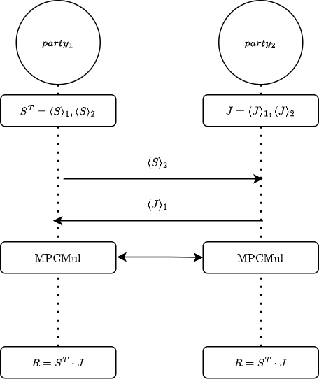
(a) PPIR(MPC)

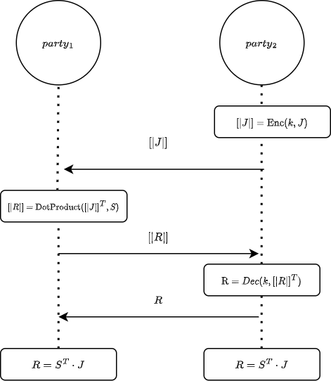
(b) PPIR(FHE)-v1

Fig. 1: Proposed framework to compute matrix-vector multiplication $S^{T}\cdot J$ based on PPIR(MPC) and PPIR(FHE)-v1.

Given images $I,J:\mathbb{R}^{d}\mapsto\mathbb{R}$, image registration aims at estimating the parameters ${\bm{\theta}}$ of a spatial transformation ${\bm{W}}_{\bm{\theta}}\in\mathbb{R}^{d}\mapsto\mathbb{R}^{d}$, either linear or non-linear, maximizing the spatial overlap between $J$ and the transformed image $I({\bm{W}}_{\bm{\theta}})$, by minimizing a distance function $f$:

$${\bm{\theta}}^{*}=\text{argmin}_{{\bm{\theta}}}~{}f\left(I({\bm{W}}_{\bm{\theta}}({\bm{x}})),J({\bm{x}})\right).$$ (1)

The distance function $f$ can be any similarity measure, e.g., the Sum of Squared Differences (SSD) or the negative Mutual Information (MI). Equation (1) can be typically optimized through gradient-based methods, where the parameters ${\bm{\theta}}$ are iteratively updated until convergence. In particular, when using a Gauss-Newton optimization scheme Algorithm 1, the parameters update of the spatial transformation can be computed through Equation (2):

$${\bm{\Delta}}{\bm{\theta}}=H^{-1}\cdot G,$$ (2)

where $G=\frac{\partial f}{\partial{\bm{\theta}}}$ is the Jacobian and $H=\frac{\partial^{2}f}{\partial{\bm{\theta}}^{2}}$ the Hessian of $f$.

We consider a scenario with two parties, $party_{1}$, and $party_{2}$, whereby $party_{1}$ owns image $I$ and $party_{2}$ owns image $J$. The parties wish to collaboratively optimize the image registration problem without disclosing their respective images to each other. We assume that only $party_{1}$ has access to the transformation parameters ${\bm{\theta}}$ and that it is also responsible for computing the update at each optimization step. In what follows, we introduce the basic notation to develop PPIR based on two similarity measures typically adopted in image registration: Sum of squared differences (SSD), and mutual information (MI).

2.1 Sum of Squared Differences

A typical cost function to be optimized during the registration process is the sum of squared intensity differences evaluated on the set of image coordinates:

$$\textsc{SSD}(I,J,{\bm{\theta}})=\text{argmin}_{{\bm{\theta}}}\sum_{{\bm{x}}}\bigg{[}I({\bm{W}}_{\bm{\theta}}({\bm{x}}))-J({\bm{x}})\bigg{]}^{2}$$ (3)

with Jacobian:

$$G=\sum_{{\bm{x}}}S({\bm{x}})\cdot(I({\bm{W}}_{\bm{\theta}}({\bm{x}}))-J({\bm{x}})),$$ (4)

where

$$S({\bm{x}})=\nabla I({\bm{x}})\frac{\partial{\bm{W}}_{\bm{\theta}}({\bm{x}})}{\partial{\bm{\theta}}}$$ (5)

quantifies image and transformation gradients, and

$$H=\sum_{{\bm{x}}}\left(\nabla I({\bm{x}})\frac{\partial{\bm{W}}_{\bm{\theta}}({\bm{x}})}{\partial{\bm{\theta}}}\right)^{T}\left(\nabla I({\bm{x}})\frac{\partial{\bm{W}}_{\bm{\theta}}({\bm{x}})}{\partial{\bm{\theta}}}\right)$$ (6)

is the second order term obtained from Equation (3) through linearization [22, 3]. The solution to this problem requires the joint availability of both images ${I}$ and ${J}$, as well as of the gradients of $I$ and of ${\bm{W}}_{\bm{\theta}}$. In a privacy-preserving setting, this information cannot be disclosed, and the computation of Equation (2) is therefore impossible. We note that to calculate the update of the registration ${\bm{\Delta}}{\bm{\theta}}$ of Equation (2), the only operation that requires the joint availability of information from both parties is the term $R=\sum_{{\bm{x}}}S({\bm{x}})\cdot J({\bm{x}})$, which can be computed a matrix-vector multiplication of vectorized quantities $R=S^{T}\cdot J$.

2.2 Mutual Information

Mutual Information quantifies the joint information content between the intensity distributions of the two images. This is calculated from the joint probability distribution function (PDF):

$$MI(I,J,{\bm{\theta}})=\text{argmin}_{{\bm{\theta}}}-\sum_{r,t}p(r,t;{\bm{\theta}})\log\left(\frac{p(r,t;{\bm{\theta}})}{p(r;{\bm{\theta}})p(t)}\right)$$ (7)

where, given $N_{r}$ and $N_{t}$ the maximum intensity respectively for $I$ and $J$, we define $r\in[0;N_{r}-1]\subseteq\mathbb{N}$ and $t\in[0;N_{t}-1]\subseteq\mathbb{N}$ as the range of discretized intensity values of $I$ and $J$, respectively. A Parzen window [21] is used to generate continuous estimates of the underlying intensity distributions, thereby reducing the effects of quantization from interpolation, and discretization from binning the data. Let $\psi_{I}^{3}:\mathbb{R}\mapsto\left[0,1\right]$ be a cubic spline Parzen window, and let $\psi_{J}^{0}:\mathbb{R}\mapsto\left[0,1\right]$ be a zero-order spline Parzen window. The smoothed joint histogram of $I$ and $J$ [29, 18] is given by:

$$p(r,t;{\bm{\theta}})=$$

$${\frac{1}{N_{{\bm{x}}}}}\sum_{{\bm{x}}}\psi_{I}^{3}\left(r-\frac{I({\bm{W}}_{\bm{\theta}}({\bm{x}}))-I({\bm{W}}_{\bm{\theta}}({\bm{x}}))^{\circ}}{\mathbf{\Delta}b_{r}}\right)\cdot\psi_{J}^{0}\left(t-\frac{J({\bm{x}})-J^{\circ}}{\mathbf{\Delta}b_{t}}\right)$$

In the above formula, the intensity values of $I$ and $J$ are normalized by their respective minimum (denoted by $I({\bm{W}}_{\bm{\theta}})^{\circ}$ and $J^{\circ}$), and by the bin size (respectively $\mathbf{\Delta}b_{r}$ and $\mathbf{\Delta}b_{t}$), to fit into the specified number of bins ($b_{r}$ or $b_{t}$) of the intensity distribution. The final value for $p(r,t;{\bm{\theta}})$ is computed by normalizing by $N_{{\bm{x}}}$, the number of sampled voxels. Marginal probabilities are simply obtained by summing along one axis of the PDF, that is, $p(r)=\sum_{t}p(r,t;{\bm{\theta}})$ and $p(t)=\sum_{r}p(r,t;{\bm{\theta}})$. Let the matrices $A_{I}^{3}\in\mathbb{R}^{N_{{\bm{x}}}\times N_{r}}$ and $B_{J}^{0}\in\mathbb{R}^{N_{{\bm{x}}}\times N_{t}}$ be defined as:

$$A_{I}^{3}({\bm{x}},r;{\bm{\theta}})=\psi_{I}^{3}\left(r-\frac{I({\bm{W}}_{\bm{\theta}}({\bm{x}}))-I({\bm{W}}_{\bm{\theta}})^{\circ}}{\mathbf{\Delta}b_{r}}\right)$$

and

$$B_{J}^{0}({\bm{x}},t)=\psi_{J}^{0}\left(t-\frac{J({\bm{x}})-J^{\circ}}{\mathbf{\Delta}b_{t}}\right),$$

the discretized joint PDF can be rewritten in a matrix form via the multiplication:

$$P={\frac{1}{N_{{\bm{x}}}}}\cdot(A_{I}^{3})^{T}\cdot B_{J}^{0}$$ (8)

The first derivative of the joint PDF is calculated as follows [10]:

$$\frac{\partial p(r,t;{\bm{\theta}})}{\partial{\bm{\theta}}}=-\frac{1}{N_{{\bm{x}}}}\cdot\sum_{{\bm{x}}}B_{J}^{0}({\bm{x}},t)\cdot\frac{\partial\psi_{I}^{3}(\epsilon)}{\partial\epsilon}\cdot\frac{\partial\epsilon}{\partial I({\bm{W}}_{\bm{\theta}}({\bm{x}}))}\cdot\frac{\partial I({\bm{W}}_{\bm{\theta}}({\bm{x}}))}{\partial{\bm{\theta}}}$$

where $\epsilon=\epsilon({\bm{x}},r;{\bm{\theta}})=r-\frac{I({\bm{W}}_{\bm{\theta}}({\bm{x}}))-I({\bm{W}}_{\bm{\theta}})^{\circ}}{\mathbf{\Delta}b_{r}}$ is the input of the cubic spline. We also introduce the matrix $C_{I}^{3}\in\mathbb{R}^{N_{{\bm{x}}}\times N_{r}}$ defined as $C_{I}^{3}({\bm{x}},r;{\bm{\theta}})=\frac{\partial\psi_{I}^{3}(\epsilon)}{\partial\epsilon}\cdot\frac{\partial\epsilon}{\partial I({\bm{W}}_{\bm{\theta}}({\bm{x}}))}\cdot\frac{\partial I({\bm{W}}_{\bm{\theta}}({\bm{x}}))}{\partial{\bm{\theta}}}$, to write the discretized first derivative as the matrix:

$$P^{\prime}=-\frac{1}{N_{{\bm{x}}}}\cdot(B_{J}^{0})^{T}\cdot C_{I}^{3}$$ (9)

The Jacobian of the MI is obtained from the chain rule and takes the form:

$$G=\sum_{r,t}{\frac{\partial p(r,t;{\bm{\theta}})}{\partial{{\bm{\theta}}}}}\log\left(\frac{p(r,t;{\bm{\theta}})}{p(r;{\bm{\theta}})}\right)$$

while the linearized Hessian [11] can be written as:

$$H=\sum_{r,t}\left\{{\frac{\partial p(r,t;{\bm{\theta}})}{\partial{{\bm{\theta}}}}}^{T}\frac{\partial p(r,t;{\bm{\theta}})}{\partial{{\bm{\theta}}}}\left(\frac{1}{p(r,t;{\bm{\theta}})}-\frac{1}{p(r;{\bm{\theta}})}\right)\right\},$$

The derivatives can be easily calculated from the properties of B-splines since we have $\frac{\partial\psi_{I}^{3}}{\partial\epsilon}=\psi^{2}_{I}(\epsilon+\frac{1}{2})-\psi^{2}_{I}(\epsilon-\frac{1}{2})$. In a privacy-preserving scenario, to calculate the update of the registration ${\bm{\Delta}}{\bm{\theta}}$ of Equation (7), two operations require the joint availability of information from both parties, which are the matrix $P$ of Equation (8) and the matrix $P^{\prime}$ of Equation (9).

2.3 Secure Computation

After introducing in Section 1 the optimization problem and the related functionals, in this section, we review the standard privacy-preserving techniques that will be employed to develop our PPIR.

2.4 Secure Multi-Party Computation

Introduced by Yao [30], MPC is a cryptographic tool that allows multiple parties to jointly compute a common function over their private inputs (secrets) and discover no more than the output of this function. Among existing MPC protocols, additive secret sharing consists of first splitting every secret $s$ into additive shares $\langle s\rangle_{i}$, such that $\sum_{i=1}^{n}\langle s\rangle_{i}=s$, where $n$ is the number of collaborating parties. Each party $i$ receives one share $\langle s\rangle_{i}$ and executes an arithmetic circuit in order to obtain the final output of the function. In this paper, we adopt the two-party computation protocol defined in SPDZ [9], whereby the actual function is mapped into an arithmetic circuit and all computations are performed within a finite ring with modulus $Q$. Additions consist of locally adding shares of secrets, while multiplications require interaction between parties. Following [9], SPDZ defines a dedicated MPCMul to compute matrix-vector multiplication and MPCMatMul to compute matrix-matrix multiplication. These operations are performed within an honest but curious protocol.

2.5 Homomorphic Encryption

Initially introduced by Rivest et al. in [24], Homomorphic Encryption (HE) enables the execution of operations over encrypted data without disclosing either the input data or the result of the computation. Hence, $party_{1}$ encrypts the input with its public key and sends the encrypted input to $party_{2}$. In turn, $party_{2}$ evaluates a circuit over this encrypted input and sends the result, which still remains encrypted, back to $party_{1}$ which can finally decrypt them. Among various HE schemes, CKKS [7] supports the execution of all operations on encrypted real values and is considered a levelled homomorphic encryption (LHE) scheme. The supported operations are: Sum (+), Element-wise multiplication ($\ast$) and DotProduct. With CKKS, an input vector is mapped to a polynomial and further encrypted with a public key in order to obtain a pair of polynomials $c=(c_{0},c_{1})$. The original function is further mapped into a set of operations that are supported by CKKS, which are executed over $c$. The performance and security of CKKS depend on multiple parameters including the degree of the polynomial $N$, which is usually sufficiently large (e.g. $N=4096$, or $N=8192$).

3 Methods

We propose two versions of PPIR according to the underlying cryptographic tool, namely PPIR(MPC), integrating MPC, and PPIR(FHE), integrating FHE. As previously mentioned, the operations of SSD and MI are first revisited in order to be compatible with cryptographic tools. To this end, in the following sections, we first integrate the secure optimization of these two metrics separately and then propose improvements to the protocols to enhance scalability when applied to large-dimensional imaging information.

3.1 PPIR based on SSD

As mentioned in Section 2.1, when optimizing the SSD cost, the only sensitive operation that must be jointly executed by the parties is the matrix-vector multiplication: $R=S^{T}\cdot J$, where $S^{T}$ is only known to $party_{1}$ and $J$ to $party_{2}$. Figure 1 illustrates how cryptographic tools are employed to ensure privacy during registration.

With MPC (Figure 1(a)), $party_{1}$ secretly shares the matrix $S^{T}$ to obtain $(\langle S\rangle_{1},\langle S\rangle_{2})$, while $party_{2}$ secretly shares the image $J$ to obtain $(\langle J\rangle_{1},\langle J\rangle_{2})$. Each party also receives its corresponding share, so that $party_{1}$ holds ($\langle S\rangle_{1},\langle J\rangle_{1})$ and $party_{2}$ holds $(\langle S\rangle_{2},\langle J\rangle_{2})$. The parties execute a circuit with MPCMul operations to calculate the 2-party dot product between $S^{T}$ and $J$. The parties further synchronize to allow $party_{1}$ to obtain the product and finally to calculate ${\bm{\Delta}}{\bm{\theta}}$ (Equations (4) and (6)).

When using FHE (Figure 1(b)), $party_{2}$ first uses a FHE key $k$ to encrypt ${J}$ and obtains $\llbracket{J}\rrbracket\leftarrow\textsc{Enc}(k,{J})$. This encrypted image is sent to $party_{1}$, who computes the encrypted matrix-vector multiplication $\llbracket R\rrbracket$. In this framework, only vector $J$ is encrypted, and therefore $party_{1}$ executes scalar multiplications and additions in the encrypted domain only (which are less costly than multiplications over two encrypted inputs). The encrypted result $\llbracket R\rrbracket$ is sent back to $party_{2}$, which can obtain the result by decryption: $R=\textsc{Dec}(k,\llbracket R\rrbracket)$. Finally, $party_{1}$ receives $R$ in clear form and can therefore compute ${\bm{\Delta}}{\bm{\theta}}$.

Thanks to the privacy and security guarantees of these cryptographic tools, during the entire registration procedure, the content of the image data $S$ and $J$ is never disclosed to the opposite party.

3.2 PPIR based on MI

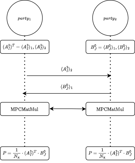
(a) PPIR(MPC)

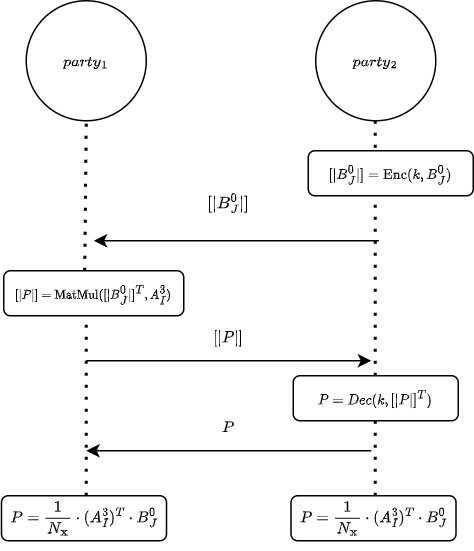
(b) PPIR(FHE)

Fig. 2: Proposed framework to calculate matrix multiplication $P=\frac{1}{N_{{\bm{x}}}}\cdot(A_{I}^{3})^{T}\cdot B_{J}^{0}$ based on PPIR(MPC) and PPIR(FHE).

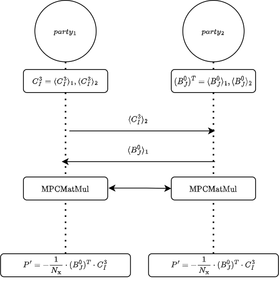
(a) PPIR(MPC)

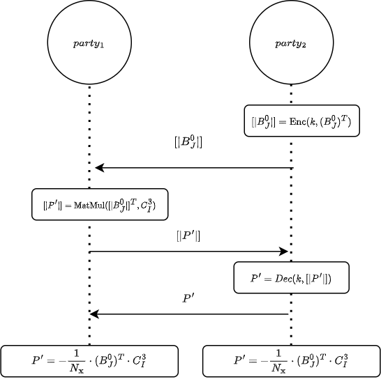
(b) PPIR(FHE)

Fig. 3: Proposed framework to calculate matrix multiplication $P^{\prime}=-\frac{1}{N_{{\bm{x}}}}\cdot(B_{J}^{0})^{T}\cdot C_{I}^{3}$ based on PPIR(MPC) and PPIR(FHE).

Figure 2(a) shows the MPC variant to calculate the joint PDF $P$ in a privacy-preserving manner, where $A_{I}^{3}$ is only known to $party_{1}$ and $B_{J}^{0}$ to $party_{2}$. Initially: $party_{1}$ secretly shares matrix $(A^{3}_{I})^{T}=(\langle A_{I}^{3}\rangle_{1},\langle A_{I}^{3}\rangle_{2})$, while $party_{2}$ does the same with $B_{J}^{0}=(\langle B_{J}^{0}\rangle_{1},\langle B_{J}^{0}\rangle_{2})$. Each party also receives its corresponding share: $party_{1}$ now holds $(\langle A_{I}^{3}\rangle_{1},\langle B_{J}^{0}\rangle_{1})$, and $party_{2}$ holds $(\langle B_{J}^{0}\rangle_{2},\langle A_{I}^{3}\rangle_{2})$. The parties execute a circuit with MPCMatMul operation to calculate the 2-party matrix multiplication between $(A_{I}^{3})^{T}$ and $B_{J}^{0}$. The next operation carried out in the privacy-preserving setting is the computation of the first derivative of Equation (9). Figure 3(a) illustrates the MPC variant, where $party_{1}$ only knows $C^{3}_{I}$ and $party_{2}$ only knows $B^{0}_{J}$. Initially, $party_{1}$ secretly shares the matrix $C^{3}_{I}=(\langle C^{3}_{I}\rangle_{1},\langle C^{3}_{I}\rangle_{2})$, while $party_{2}$ does the same with $(B^{0}_{J})^{T}=(\langle B^{0}_{J}\rangle_{1},\langle B^{0}_{J}\rangle_{2})$. Each party also receives its corresponding share, namely: $party_{1}$ holds $(\langle C^{3}_{I}\rangle_{1},\langle B^{0}_{J}\rangle_{1})$ and $party_{2}$ holds $(\langle C^{3}_{I}\rangle_{2},\langle B^{0}_{J}\rangle_{2})$. The parties also execute a circuit with the MPCMatMul between $(B^{0}_{J})^{T}$ and $C^{3}_{I}$. Likewise MPC, we define the FHE variant, (Figure 3(b)), where $party_{2}$ uses an FHE key $k$ to compute $\llbracket{B_{J}^{0}}\rrbracket\leftarrow\textsc{Enc}(k,{B_{J}^{0}})$. Then $\llbracket{B_{J}^{0}}\rrbracket$ is sent to $party_{1}$, which computes the joint PDF $P$ as a matrix multiplication between $A_{I}^{3}$ and the encrypted $\llbracket B_{J}^{0}\rrbracket$. The encrypted result $\llbracket P\rrbracket$ is sent back to $party_{2}$, which can obtain the result by decryption: $P=\textsc{Dec}(k,\llbracket P\rrbracket^{T})$. Finally, $party_{1}$ receives $P$ in clear form. The FHE variant for the first derivative matrix $P^{\prime}$ is similar to the FHE approach for the joint PDF matrix $P$, (Figure 3(b)).

3.3 Protocols enhancement

Effectively optimizing Equation (1) with MPC or FHE is particularly challenging, due to the computational bottleneck of these techniques when applied to large-dimensional objects [14, 4], notably affecting the computation time and the occupation of communication bandwidth between parties. Because cryptographic tools introduce a non-negligible overhead in terms of performance and scalability, in this section we introduce specific techniques to optimize the underlying image registration operations.

3.3.1 Gradient sampling

Since the registration gradient is generally driven mainly by a fraction of the image content, such as the image boundaries in the case of SSD cost, a reasonable approximation of Equations (4) and (6) can be obtained by evaluating the cost only on relevant image locations. This idea has been introduced in medical image registration [29, 18, 26], and here is adopted to optimize Equation (3) by reducing the dimensionality of the arrays on which encryption is performed. We test two different techniques: (i): Uniformly Random Selection (URS), proposed by [29, 18], in which a random subset of dimension $l\leq d$ of spatial coordinates is sampled at every iteration with uniform probabilities, $p({\bm{x}})=\frac{1}{d}$; and (ii): Gradient Magnitude Sampling (GMS) [26], which consists of sampling a subset of coordinates with probability proportional to the norm of the image gradient, $p({\bm{x}})\sim\|\nabla I({\bm{x}})\|$. We note that gradient sampling is not necessary for studying the computation of MI since in Equation (8) the computation is already performed on a subsample of the image voxels.

3.3.2 Matrix partitioning in FHE

We now describe additional improvements dedicated to PPIR(FHE) and propose two versions of this solution: (i) PPIR(FHE)-v1 implements an optimization of the matrix-vector multiplication by partitioning the vector image into a vector of submatrices, whereas (ii) PPIR(FHE)-v2 enhances the workload of the parties by fairly distributing the computation among them.

PPIR(FHE)-v1

We introduce here a novel optimization dedicated to PPIR with FHE, in particular when the CKKS algorithm is adopted. CKKS allows multiple inputs to be packed into a single ciphertext to decrease the number of homomorphic operations. To optimize matrix-vector multiplication, we propose to partition the image vector $J$ into $k$ sub-arrays of dimension $l$, and the matrix $S^{T}$ into $k$ sub-matrices of dimension $|{\bm{\theta}}|\times l$. Once all sub-arrays $J_{i}$ are encrypted, we propose to iteratively apply DotProduct as proposed by Benaissa et al. [4], between each sub-matrix and corresponding sub-array; these intermediate results are then summed to obtain the final result, namely: $\llbracket R\rrbracket=\sum_{i=0}^{K}\textsc{DotProduct}\left(\llbracket J_{i}^{T}\rrbracket,S_{i}\right)=S^{T}\cdot\llbracket J\rrbracket$.

PPIR(FHE)-v2

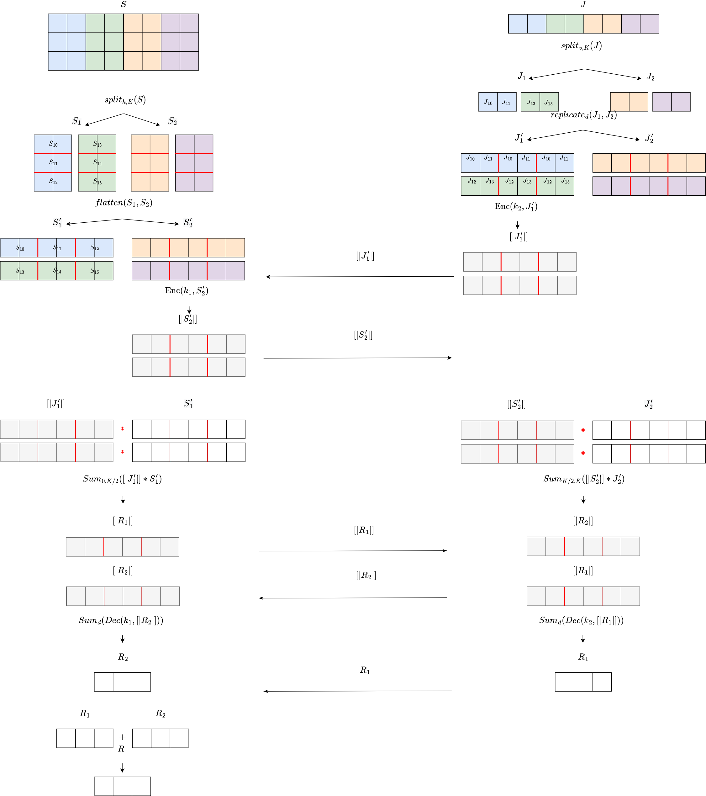
Fig. 4: Proposed framework to compute matrix-vector multiplication $S^{T}\cdot J$ based on PPIR(FHE)-v2.

In addition to packing multiple inputs into a single ciphertext, the application of FHE to PPIR can be optimized by more equally distributing the workload among the two parties. We note that in PPIR(FHE)-v1, $party_{1}$ is in charge of computing the matrix-vector multiplication entirely while $party_{2}$ only encrypts the input and decrypts the result. Following Appendix Figure 4, PPIR(FHE)-v2 starts by splitting the matrix $S$ of $party_{1}$ into two sub-matrices $S_{1}$ and $S_{2}$ using the operation $split_{h,K}$. This operation partitions the matrix into K equally-sized sub-matrices. Next, the operation $flatten$ is applied to $S_{1}$ and $S_{2}$, obtaining vectors $S_{1}^{\prime}$ and $S_{2}^{\prime}$ respectively. Then, $party_{1}$ encrypts $S_{2}^{\prime}$ and sends it to $party_{2}$, which subsequently applies to its vector $J$ the operation $split_{v,K}$, obtaining $J_{1}$ and $J_{2}$. This operation splits $J$ into $K$ equally-sized partitions, and it executes the operation $replicate_{d}$ to $J_{1}$ and $J_{2}$, obtaining $J^{\prime}_{1}$ and $J^{\prime}_{2}$ respectively. $party_{2}$ encrypts $J_{1}^{\prime}$ and sends it to $party_{1}$. Both parties then iteratively perform the element-wise multiplication $\ast$ and sum up the results of the different partitions using the primitive $Sum_{i,k}$. The protocol doesn’t rely anymore on DotProduct and leads to a significant gain in computational load.

4 Experiments & Results

SSD Affine registration and efficiency metrics
Solution	Intensity Error (SSD)	Num. Interation	Displacement RMSE ($mm$)	Time $party_{1}$ (s)	Time $party_{2}$ (s)	Comm. $party_{1}$ (MB)	Comm. $party_{2}$ (MB)
Clear	$4.34\pm 0.0$	$118\pm 0.0$	-	$0.0$	$0.0$	-	-
PPIR(MPC)	$4.34\pm 0.0$	$114.8\pm 4.0$	$0.13\pm 0.04$	$0.13$	$0.13$	$1.54$	$1.54$
Clear + URS	$4.38\pm 0.0$	$61\pm 0.0$	-	$0.0$	$0.0$	-	-
PPIR(MPC) + URS	$4.34\pm 0.0$	$60.4\pm 6.85$	$1.75\pm 0.19$	$0.02$	$0.02$	$0.20$	$0.20$
PPIR(FHE)-v1 ($D=128$) + URS	$4.34\pm 0.10$	$61.80\pm 4.82$	$13.47\pm 2.87$	$2.55$	$0.02$	$0.06$	$0.01$
PPIR(FHE)-v2 ($D=128$) + URS	$4.34\pm 0.10$	$61.60\pm 7.21$	$13.93\pm 4.28$	$0.01$	$0.02$	$0.72$	$0.88$
Clear + GMS	$4.34\pm 0.0$	$63\pm 0.0$	-	$0.0$	$0.0$	-	-
PPIR(MPC) + GMS	$4.34\pm 0.0$	$59.80\pm 6.20$	$0.93\pm 0.42$	$0.02$	$0.02$	$0.20$	$0.20$
PPIR(FHE)-v1 ($D=128$) + GMS	$4.34\pm 0.05$	$60.40\pm 5.12$	$0.59\pm 0.35$	$2.51$	$0.02$	$0.06$	$0.01$
PPIR(FHE)-v2 ($D=128$) + GMS	$4.34\pm 0.05$	$57.03\pm 4.07$	$0.50\pm 0.36$	$0.02$	$0.02$	$0.73$	$0.93$

Table 1: Affine SSD registration test. Registration metrics are reported as mean and standard deviation. Efficiency metrics in terms of average across iterations. RMSE: root mean square error.

We demonstrate and assess PPIR in two examples based on the linear and non-linear alignment of positron emission tomography (PET) data, and brain scans from anatomical magnetic resonance images space(MRIs). Experiments are carried out on both 2D and 3D imaging data.

4.1 Dataset

PET data consists of 18-Fluoro-Deoxy-Glucose (${}^{18}FDG$) whole body Positron Emission Tomography (PET). The images here considered are a frontal view of the maximum intensity projection reconstruction, obtained by 2D projection of the voxels with the highest intensity across views ($1260\times 1090$ pixels). Brain MRIs are obtained from the Alzheimer’s Disease Neuroimaging Initiative [20]. The images were processed via a standard processing pipeline to estimate density maps of gray matter [1]. The subsequent registration experiments in 2D are performed on the extracted mid-coronal slice, of dimension $121\times 121$ pixels. For 3D multimodal registration, we use both MR images and PET images from the ADNI dataset, where their size are respectively $180\times 256\times 256$ voxels for the MR images and $160\times 160\times 96$ voxels for the PET images.

4.2 Implementation

In order to avoid local minima and to decrease computation time, we use a hierarchical multiresolution optimization scheme. The scheme involves $M$ resolution steps, denoted as $r_{1}\ldots r_{M}$. At each resolution step $r_{m}$, the input data is downsampled by a scaling factor $m$, where $m\in[1\ldots M]$. The quality of PPIR is assessed by comparing the registration results with those obtained with standard registration on clear images (Clear). The metrics considered are the difference in image intensity at optimum (for SSD), the total number of iterations required to converge, and the displacement root mean square difference (RMSE) between Clear and PPIR. We also evaluate the performance of PPIR in terms of average computation (running time) and communication (bandwidth) across iterations.

SSD Evaluation

Whole-body PET image alignment was first performed by optimizing the transformation ${\bm{W}}_{\bm{\theta}}$ in Equation (1) with respect to affine registration parameters. The multiresolution steps used are $r_{1},r_{5},r_{10},r_{20}$. The registration of brain gray matter density images was performed by non-linear registration without gradient approximation based on a cubic spline model (one control point every five pixels along both dimensions), with multiresolution steps $r_{1}$ and $r_{2}$. A second whole-body PET image alignment experiment was performed by non-linear registration, without gradient approximation based on a cubic spline model (one control point every four pixels along both dimensions), with multiresolution steps $r_{1}$,$r_{2}$,$r_{5}$,$r_{10}$,$r_{20}$ and $r_{30}$. Concerning the PPIR framework, transformations were optimized for both MPC and FHE by using gradient approximation (Section 3) using the same sampling seed for each test. For MPC we set as the prime modulus $Q=2^{32}$. For PPIR(FHE), we define the polynomial degree modulus as $N=4096$, and set the resizing parameter $D$ to optimize the trade-off between run-time and bandwidth. Since $D$ needs to be a divisor of the image size, for PET image data we set $D=128$, while for gray matter images, we set $D=121$ and $D=128$ for the PET images.

Mutual Information Evaluation

We tested PPIR with MI for multi-modal 3D affine image registration between PET and MRI brain scans where, in addition to varying the multi-resolution steps, a Gaussian blurring filter is applied to the images with a kernel that narrows as multi-resolution proceeds. The kernel size at different resolutions, denoted with $\sigma_{1}\ldots\sigma_{M}$, is used to control the amount of blurring applied to the image at each step of the multi-resolution process. The multiresolution steps applied are $r_{5}$ and $r_{10}$, with $10\%$ of the image’s pixels utilized as the number of subsample pixels ($N_{{\bm{x}}}$). Gaussian image blurring is applied with a degree of $\sigma_{5}=1$ and $\sigma_{10}=3$. The experimental results here are based on affine PPIR(MPC) since, due to high runtime complexity, it was not possible to optimize PPIR(FHE) compatibly with our computational budget.

Implementation Details

The PPIR framework is implemented using two state-of-the-art libraries: PySyft [25], which provides SPDZ two-party computation, and TenSeal [4], which implements the CKKS protocol. PPIR based on MI is implemented by extending the Dipy framework of Garyfallidis et al. [12]. All the experiments are executed on a machine with an Intel(R) Core(TM) i7-7800X CPU @ (3.50GHz x 12) using 132GB of RAM. For each registration configuration, the optimization is repeated 10 times to account for the random generation of MPC shares and FHE encryption keys. The code is released in a GitHub repository. We used Weights & Biases [5], for the experiment tracking, and the links of our tracked results are available in the GitHub repository.

SSD Cubic splines registration metrics
Solution	Intensity Error (SSD)	Num. Interation	Displacement RMSE ($mm$)	Time $party_{1}$ (s)	Time $party_{2}$ (s)	Comm. $party_{1}$ (MB)	Comm. $party_{2}$ (MB)
Clear	$0.65\pm 0.0$	$413\pm 0.0$	-	$0.0$	$0.0$	-	-
PPIR-MPC	$0.65\pm 0.0$	$345.70\pm 91.22$	$7.31\pm 1.86$	$0.63$	$0.63$	$21.47$	$28.98$
PPIR(FHE)-v1($D=128$)	$0.64\pm 0.0$	$224.7\pm 79.15$	$9.50\pm 4.34$	$3.41$	$0.00$	$0.06$	$0.01$
PPIR(FHE)-v2($D=256$)	$0.64\pm 0.0$	$379.2\pm 75.82$	$11.02\pm 4.93$	$0.98$	$0.43$	$40.45$	$3.56$
Clear + URS	$0.02\pm 0.0$	$101\pm 0.0$	-	$0.0$	$0.0$	-	-
PPIR(MPC) + URS	$0.02\pm 0.00$	$79.3\pm 1.88$	$5.59\pm 0.39$	$0.41$	$0.41$	$8.00$	$8.00$
PPIR(FHE)-v1($D=128$) + URS	$0.02\pm 0.00$	$105.40\pm 1.71$	$7.63\pm 0.01$	$12.23$	$0.0$	$0.06$	$0.01$
PPIR(FHE)-v2($D=128$) + URS	$0.02\pm 0.00$	$105.20\pm 2.54$	$8.74\pm 1.90$	$0.62$	$0.26$	$24.74$	$3.37$
Clear + GMS	$0.02\pm 0.0$	$103.00\pm 0.0$	-	$0.0$	$0.0$
PPIR(MPC) + GMS	$0.02\pm 0.04$	$80.20\pm 1.62$	$6.17\pm 0.37$	$0.41$	$0.41$	$8.00$	$8.00$
PPIR(FHE)-v1($D=128$) + GMS	$0.02\pm 0.00$	$105.70\pm 2.40$	$5.60\pm 2.22$	$11.95$	$0.0$	$0.06$	$0.01$
PPIR(FHE)-v2($D=128$) + GMS	$0.02\pm 0.00$	$106.32\pm 1.30$	$9.11\pm 2.34$	$0.62$	$0.26$	$24.91$	$3.35$

Table 2: Non-Linear SSD registration test. The registration metrics are reported as mean and standard deviation. Efficiency metrics in terms of average across iterations. RMSE: root mean square error.

MI Affine registration metrics (a) Solution Intensity Error (MI) Num. Iteration Displacement RMSE ($mm$) Clear 0.2208 321 - PPIR(MPC) $0.2190\pm 0.0$ $206\pm 4.0$ $1.84\pm 0.20$
MI - Joint PDF efficency metrics (b) Solution Time $party_{1}$ (s) Time $party_{2}$ (s) Comm. $party_{1}$ (MB) Comm. $party_{2}$ (MB) Clear 0.0 0.0 - - PPIR(MPC) 0.05 0.05 2206.92 2508.16	MI - First Derivative Joint PDF efficiency metrics (c) Solution Time $party_{1}$ (s) Time $party_{2}$ (s) Comm. $party_{1}$ (MB) Comm. $party_{2}$ (MB) Clear 0.0 0.0 - - PPIR(MPC) 0.75 0.75 2235.953 2540.392

Table 3: Affine MI registration test. Registration metrics are reported as mean and standard deviation. Efficiency metrics in terms of average across iterations. RMSE: root mean square error.

4.3 Results

SSD Results

Table 1 (Registration metrics) shows that affine PPIR of whole body PET images through PPIR(MPC) leads to negligible differences with respect to Clear in terms of the number of iterations, intensity, and displacement. Registration with PPIR(FHE) is instead not possible when considering the entire images, due to computational complexity, while using URS and GMS is associated to generally larger approximations. Nevertheless, Figure 5 in Appendix shows that neither MPC nor FHE decreases the overall quality of the affine registered images. A comprehensive assessment of the registration results is available in Appendix. Table 1 (Efficiency metrics) shows that PPIR(MPC) performed on full images requires the highest computation time and required communication bandwidth. These numbers improve sensibly when using URS or GMS (by factors $10\times$ and $20\times$ for time and bandwidth, respectively). Concerning PPIR(FHE)-v1, we note the uneven computation time and bandwidth usage between clients, due to the asymmetry of the encryption operations and communication protocol (Figure 1). PPIR(FHE)-v2, which shares the computational workload between the two parties and avoids DotProduct, allows obtaining an important speed-up over PPIR(FHE)-v1 ($100\times$ faster). Notably, this gain is obtained without affecting the quality of the registration metrics, and imrpoves the execution time at the levels of PPIR(MPC). On the other side, although PPIR(FHE)-v1 is able to improve communication with respect to PPIR(MPC), it still suffers from the highest bandwidth among the three proposed solutions. This is due to the fact PPIR(FHE) protocols can find different applications depending on the requirements in terms of computational power or bandwidth.

Table 2 reports the metrics for the non-linear registration test on brain density images. Regarding the accuracy of the registration, we draw conclusions similar to those of the affine case, where PPIR(MPC) leads to minimum differences with respect to Clear, while PPIR(FHE)-v1 seems slightly superior. PPIR(MPC) is associated with a lower execution time and a higher computational bandwidth, due to the larger number of parameters of the cubic splines, which affects the size of the matrix $S$. Although PPIR(FHE)-v1 has a slower execution time, the demanded bandwidth is inferior to the one of PPIR(MPC), since the encrypted image is transmitted only once. PPIR(FHE)-v2, as in the affine case, outperforms PPIR(FHE)-v1 (still about $100\times$ faster) leading to comparable values between registration metrics and is still inferior to PPIR(MPC). Here, the limitations of PPIR(FHE)-v1 on the bandwidth size are even more evident than in the affine case, since the bandwidth increases according to the number of parameters. This result gives a non-negligible burden to the $party_{1}$, due to the multiple sending of the flattened and encrypted submatrices of updated parameters. Furthermore, in this case, PPIR(FHE)-v1 performs slightly worse than PPIR(MPC) in terms of execution time. Finally, the qualitative results, reported in Appendix (6), show negligible differences between images transformed with Clear, PPIR(MPC) and PPIR(FHE)-v1.

MI Results

Table 3 reports the cost of computing the protocol for the joint PDF and the First Derivative of the Joint PDF, with Clear and by using PPIR(MPC), MI Affine registration metrics (a). MI - Joint PDF efficiency metrics (b) shows the cost of computing on 3D images the joint PDF $p$ with PPIR(MPC), while MI - First Derivative Joint PDF efficiency metrics (c) reports the same metrics assessed for the computation of the matrix-tensor multiplication of Equation (9) on 3D images. The relevant bandwidth demand is justified by the large dimension of the matrices $A_{I}^{3}$, $B_{J}^{0}$ and $C_{I}^{0}$. Qualitative results for the image registration are shown in Figure 7 in Appendix, indicating that there is no difference between the moving transformed using Clear and PPIR(MPC).

5 Conclusion

This work presents a novel framework, Privacy Preserving Image Registration (PPIR), that allows image registration when images are confidential and cannot be disclosed in clear. The PPIR framework is developed using secure multi-party computation (MPC) and Fully Homomorphic Encryption (FHE), and effectively addresses the known computational and communication overhead challenges of these techniques. We have demonstrated and evaluated the performance of PPIR with different cost functions, through a series of quantitative and qualitative benchmarks in both linear and non-linear image registration problems. Our results highlight the trade-off between registration performance and efficiency of the different PPIR schemes.

As future work, we plan to extend PPIR to other cost functions used in image registration to broaden its applicability.

Appendix

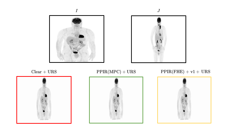
Fig. 5: Qualitative results for affine registration with SSD. The red frame is the transformed moving image using Clear+URS registration. Green and Yellow frames are the transformed images using respectively PPIR(MPC)+URS and PPIR(FHE)-v1+URS.

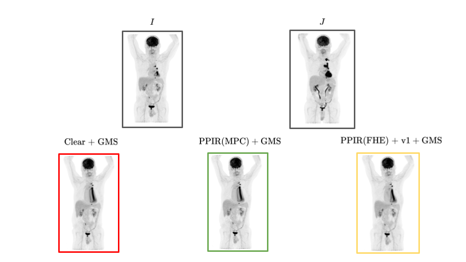
Fig. 6: Qualitative results for Cubic splines registration with SSD. The red frame is the transformed moving image using Clear+GMS registration. Green and Yellow frames are the transformed images using respectively PPIR(MPC)+GMS and PPIR(FHE)-v1+GMS.

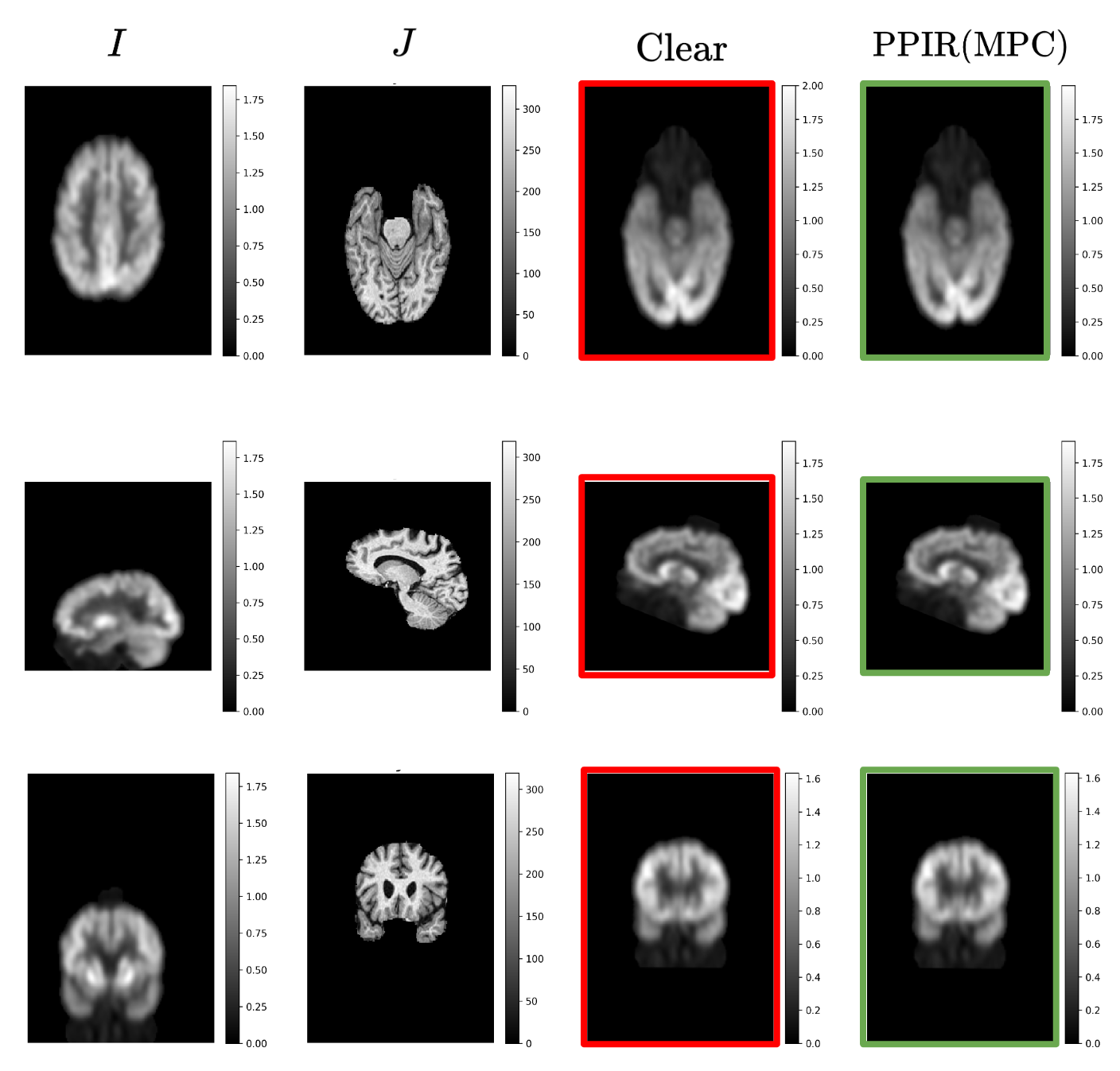
Fig. 7: Qualitative results for affine registration with MI over 3D medical images. The images are presented in a $3\times 4$ grid, with the first row representing the axial axis, the second row the sagittal axis, and the third row the coronal axis. In the first column of each row, the moving image obtained using PET modality is shown, while in the second column, the fixed image obtained using MRI modality is displayed. The third column shows the moving image transformed using Clear, while the fourth column shows the moving image transformed using PPIR(MPC). The transformed images are highlighted by red and green frames, respectively.

References

- Ashburner and Friston [2000] Ashburner, J., Friston, K.J., 2000. Voxel-based morphometry—the methods. Neuroimage 11, 805–821.
- Ashburner and Ridgway [2013] Ashburner, J., Ridgway, G.R., 2013. Symmetric diffeomorphic modeling of longitudinal structural MRI. Frontiers in neuroscience 6, 197.
- Baker and Matthews [2004] Baker, S., Matthews, I., 2004. Lucas-Kanade 20 years on: A unifying framework. International journal of computer vision 56, 221–255.
- Benaissa et al. [2021] Benaissa, A., Retiat, B., Cebere, B., Belfedhal, A.E., 2021. Tenseal: A library for encrypted tensor operations using homomorphic encryption. arXiv preprint arXiv:2104.03152 .
- Biewald [2020] Biewald, L., 2020. Experiment tracking with weights and biases. URL: https://www.wandb.com/. software available from wandb.com.
- Cardoso et al. [2013] Cardoso, M.J., Leung, K., Modat, M., Keihaninejad, S., Cash, D., Barnes, J., Fox, N.C., Ourselin, S., Initiative, A.D.N., et al., 2013. STEPs: Similarity and truth estimation for propagated segmentations and its application to hippocampal segmentation and brain parcelation. Medical image analysis 17, 671–684.
- Cheon et al. [2017] Cheon, J.H., Kim, A., Kim, M., Song, Y., 2017. Homomorphic encryption for arithmetic of approximate numbers, in: International Conference on the Theory and Application of Cryptology and Information Security, Springer. pp. 409–437.
- Dale et al. [1999] Dale, A.M., Fischl, B., Sereno, M.I., 1999. Cortical surface-based analysis: I. segmentation and surface reconstruction. Neuroimage 9, 179–194.
- Damgard et al. [2011] Damgard, I., Pastro, V., Smart, N., Zakarias, S., 2011. Multiparty computation from somewhat homomorphic encryption. Cryptology, ePrint Archive, Report 2011/535. https://ia.cr/2011/535.
- Dowson and Bowden [2006] Dowson, N., Bowden, R., 2006. A unifying framework for mutual information methods for use in non-linear optimisation, in: European Conference on Computer Vision, Springer. pp. 365–378.
- Dowson and Bowden [2007] Dowson, N., Bowden, R., 2007. Mutual information for lucas-kanade tracking (milk): An inverse compositional formulation. IEEE transactions on pattern analysis and machine intelligence 30, 180–185.
- Garyfallidis et al. [2014] Garyfallidis, E., Brett, M., Amirbekian, B., Rokem, A., Van Der Walt, S., Descoteaux, M., Nimmo-Smith, I., Contributors, D., 2014. Dipy, a library for the analysis of diffusion mri data. Frontiers in neuroinformatics 8, 8.
- Gazula et al. [2021] Gazula, H., Holla, B., Zhang, Z., Xu, J., Verner, E., Kelly, R., Jain, S., Bharath, R.D., Barker, G.J., Basu, D., et al., 2021. Decentralized multisite vbm analysis during adolescence shows structural changes linked to age, body mass index, and smoking: a coinstac analysis. Neuroinformatics 19, 553–566.
- Haralampieva et al. [2020] Haralampieva, V., Rueckert, D., Passerat-Palmbach, J., 2020. A systematic comparison of encrypted machine learning solutions for image classification, in: Proceedings of the 2020 workshop on privacy-preserving machine learning in practice, pp. 55–59.
- Heinrich et al. [2011] Heinrich, M.P., Jenkinson, M., Bhushan, M., Matin, T., Gleeson, F.V., Brady, J.M., Schnabel, J.A., 2011. Non-local shape descriptor: A new similarity metric for deformable multi-modal registration, in: International Conference on Medical Image Computing and Computer-Assisted Intervention, Springer. pp. 541–548.
- Lauter [2021] Lauter, K., 2021. Private AI: Machine Learning on Encrypted Data. Technical Report. Eprint report https://eprint.iacr.org/2021/324.pdf.
- Lotan et al. [2020] Lotan, E., Tschider, C., Sodickson, D.K., Caplan, A.L., Bruno, M., Zhang, B., Lui, Y.W., 2020. Medical imaging and privacy in the era of artificial intelligence: myth, fallacy, and the future. Journal of the American College of Radiology 17, 1159–1162.
- Mattes et al. [2003] Mattes, D., Haynor, D.R., Vesselle, H., Lewellen, T.K., Eubank, W., 2003. Pet-ct image registration in the chest using free-form deformations. IEEE transactions on medical imaging 22, 120–128.
- McMahan et al. [2017] McMahan, B., Moore, E., Ramage, D., Hampson, S., y Arcas, B.A., 2017. Communication-efficient learning of deep networks from decentralized data, in: Artificial intelligence and statistics, PMLR. pp. 1273–1282.
- Mueller et al. [2005] Mueller, S.G., Weiner, M.W., Thal, L.J., Petersen, R.C., Jack, C., Jagust, W., Trojanowski, J.Q., Toga, A.W., Beckett, L., 2005. The alzheimer’s disease neuroimaging initiative. Neuroimaging Clinics 15, 869–877.
- Parzen [1961] Parzen, E., 1961. Mathematical considerations in the estimation of spectra. Technometrics 3, 167–190.
- Pennec et al. [1999] Pennec, X., Cachier, P., Ayache, N., 1999. Understanding the “Demon’s algorithm”: 3D non-rigid registration by gradient descent, in: International Conference on Medical Image Computing and Computer-Assisted Intervention, Springer. pp. 597–605.
- Reuter et al. [2010] Reuter, M., Rosas, H.D., Fischl, B., 2010. Highly accurate inverse consistent registration: a robust approach. Neuroimage 53, 1181–1196.
- Rivest et al. [1978] Rivest, R.L., Adleman, L., Dertouzos, M.L., et al., 1978. On data banks and privacy homomorphisms. Foundations of secure computation 4, 169–180.
- Ryffel et al. [2018] Ryffel, T., Trask, A., Dahl, M., Wagner, B., Mancuso, J., Rueckert, D., Passerat-Palmbach, J., 2018. A generic framework for privacy preserving deep learning. arXiv preprint arXiv:1811.04017 .
- Sabuncu and Ramadge [2004] Sabuncu, M.R., Ramadge, P.J., 2004. Gradient based nonuniform subsampling for information-theoretic alignment methods, in: The 26th Annual International Conference of the IEEE Engineering in Medicine and Biology Society, IEEE. pp. 1683–1686.
- Schnabel et al. [2016] Schnabel, J.A., Heinrich, M.P., Papież, B.W., Brady, J.M., 2016. Advances and challenges in deformable image registration: from image fusion to complex motion modelling. Medical Image Analysis 33, 145–148.
- Shattuck et al. [2009] Shattuck, D.W., Prasad, G., Mirza, M., Narr, K.L., Toga, A.W., 2009. Online resource for validation of brain segmentation methods. NeuroImage 45, 431–439.
- Viola and Wells III [1997] Viola, P., Wells III, W.M., 1997. Alignment by maximization of mutual information. International journal of computer vision 24, 137–154.
- Yao [1982] Yao, A.C., 1982. Protocols for secure computations, in: 23rd annual symposium on foundations of computer science (sfcs 1982), IEEE. pp. 160–164.