LeNSE: Learning To Navigate Subgraph Embeddings
for Large-Scale Combinatorial Optimisation

Abstract

Combinatorial Optimisation problems arise in several application domains and are often formulated in terms of graphs. Many of these problems are NP-hard, but exact solutions are not always needed. Several heuristics have been developed to provide near-optimal solutions; however, they do not typically scale well with the size of the graph. We propose a low-complexity approach for identifying a (possibly much smaller) subgraph of the original graph where the heuristics can be run in reasonable time and with a high likelihood of finding a global near-optimal solution. The core component of our approach is LeNSE, a reinforcement learning algorithm that learns how to navigate the space of possible subgraphs using an Euclidean subgraph embedding as its map. To solve CO problems, LeNSE is provided with a discriminative embedding trained using any existing heuristics using only on a small portion of the original graph. When tested on three problems (vertex cover, max-cut and influence maximisation) using real graphs with up to $10$ million edges, LeNSE identifies small subgraphs yielding solutions comparable to those found by running the heuristics on the entire graph, but at a fraction of the total run time. Code for the experiments is available in the public GitHub repo at https://github.com/davidireland3/LeNSE.

1 Introduction

Combinatorial optimisation (CO) problems involve the search for maxima or minima of an objective function whose domain is a discrete but large configuration space (Wolsey & Nemhauser, 1999; Korte et al., 2011; Grötschel et al., 2012). Most CO problems can be formulated naturally in terms of graphs (Avis et al., 2005; Arumugam et al., 2016; Vesselinova et al., 2020), and an optimal solution typically consists of a set of vertices that optimises the objective function. Some well-known examples are the Vertex Cover Problem (VCP) (Dinur & Safra, 2005), i.e. the problem of finding a set of vertices that includes at least one endpoint of every edge of the graph, and the Max-Cut (MC) problem (Goemans & Williamson, 1995), i.e. finding a cut whose size is at least the size of any other cut. Many CO problems have a wide range of real-world applications, e.g. in biology (Wilder et al., 2018; Reis et al., 2019), social networks (Brown & Reingen, 1987; Valente, 1996; Rogers, 2010; Chaoji et al., 2012), circuit design (Barahona et al., 1988) and auctions (Kempe et al., 2010; Dobzinski et al., 2011; Amanatidis et al., 2017).

Finding the optimal solution to a CO problem requires an exhaustive search of the solution space; with many canonical CO problems being NP-hard (Karp, 1972), this usually means that they are unsolvable in practice. However, exact optimal solutions are often not required, and many heuristic approaches have been developed to obtain near-optimal solutions in some reasonable time (Hochbaum, 1982; Goemans & Williamson, 1995; Applegate et al., 2001; Kempe et al., 2003; Karakostas, 2005; Ausiello et al., 2012). More frequently, the practical application of these algorithms involves very large graphs. This significantly increases the run time of the heuristics and, in some case, may preclude the use of such algorithms altogether, e.g. due to memory constraints.

For instance, the Influence Maximization (IM) problem consists of finding a seed set composed of vertices that maximize their influence spread over a social network, which may have millions of vertices and/or edges. A greedy algorithm proposed by Kempe et al. (2003) requires the objective function to be evaluated at every vertex in the graph; this is expensive as the expected spread of a vertex is #P-hard to evaluate (Kempe et al., 2003; Chen et al., 2010). Consequently, a large body of work has been carried out to develop more scalable algorithms (Goyal et al., 2011; Cheng et al., 2013, 2014; Cohen et al., 2014; Borgs et al., 2014; Tang et al., 2014, 2015). The current state of the art algorithm for solving IM, the Influence Maximization Martingale (IMM) algorithm (Tang et al., 2015), is also known to scale poorly to large graph instances due to its memory requirements (Arora et al., 2017).

In this work we present a general framework, based on supervised and reinforcement learning, for leveraging heuristics which have been crafted with extensive domain knowledge but may not scale well to large problem instances. Our proposed algorithm, LeNSE (Learning to Navigate Subgraph Embeddings), learns how to prune a graph, significantly reducing the size of the problem by removing vertices and edges so that the heuristic can find a nearly-optimal solution at a fraction of the time that would have been taken when using the entire graph. The motivation for our approach comes from the fact that a subgraph is an easier target to identify, compared to the exact solution; instead of finding a needle in a haystack, we instead learn how to remove parts of the haystack where the needle is unlikely to be.

The graph pruning process is framed as a sequential decision making problem, which is solved using Q-learning (Watkins & Dayan, 1992). Starting with any randomly chosen subgraph of fixed size, LeNSE sequentially modifies the current subgraph to a slightly altered one, and repeats this process until the current subgraph is deemed highly likely to contain a nearly-optimal solution. To efficiently navigate the space of possible subgraphs so that the highest quality one is reached in the fewest number of steps, LeNSE relies on a discriminative subgraph embedding as its navigation map. To learn this embedding, we make use of recent advances in geometric deep learning, and specifically graph neural networks (GNNs) with graph coarsening layers (Ying et al., 2018; Cangea et al., 2018; Lee et al., 2019; Liang et al., 2020). By construction, the position of an embedded subgraph reflects its predicted quality. LeNSE makes use of these quality estimates to learn optimal graph modifications that progressively move the subgraph towards more promising regions.

Experimentally we test LeNSE on three well-know CO problems using established heuristics. Our extensive experimental results demonstrate that LeNSE is capable of removing large parts of the graph, in terms of both vertices and edges, without any significant degradation to the performance compared to performing no pruning at all, but at a fraction of the overall run time. We also compare LeNSE to two baselines, a GNN vertex classifier and a recently introduced pruning approach (Manchanda et al., 2020). Remarkably, we show that all training can be done on some small, random sample of the problem graph whilst being able to scale up to the larger test graph at inference time. This means that all expensive computations needed to train LeNSE, such as running the heuristic to obtain a solution, are only ever done on small graphs. We also show that using LeNSE for the IM problem on a large graph give speed ups of more than 140 times compared to not doing any pruning.

2 Related work

In recent years, many machine learning based solutions have been investigated to solve CO problems (Bengio et al., 2020; Vesselinova et al., 2020; Mazyavkina et al., 2021). Recent contributions in the field have started to leverage techniques from geometric deep learning, which is concerned with the application of neural network techniques to non-Euclidean domains (Bronstein et al., 2017; Battaglia et al., 2018; Wu et al., 2020; Zhou et al., 2020). These developments have started to play an important role in learning based CO algorithms as they capture and exploit the graphical nature of problems. Many methods learn vertex/edge embeddings (Kipf & Welling, 2016; Hamilton et al., 2017; Gilmer et al., 2017; Veličković et al., 2017, 2018; Brody et al., 2021), whilst more recently methods have been explored to obtain graph level embeddings (Ying et al., 2018; Cangea et al., 2018; Lee et al., 2019; Liang et al., 2020). We now briefly review related work relying on both supervised and reinforcement learning.

Supervised learning: Attempts have been made to train a classifier to predict whether a vertex in a graph can be removed from consideration without effecting the quality of the solution found by a heuristic. For instance, the classifier can be used to prune the graph in one attempt (Sun et al., 2019, 2021) or in a multi-stage approach where the graph is repeatedly pruned (Grassia et al., 2019; Lauri et al., 2020). These methods, however, rely on hand crafted features that are typically specific to the problems they are trying to solve, whereas LeNSE works with multiple budget-constrained problems. Several other methods look to use datasets labelled by heuristics to learn solutions directly (Vinyals et al., 2015; Khalil et al., 2016; Joshi et al., 2019; Gasse et al., 2019; Liu et al., 2021); in contrast, our graph pruning approach consists of several incremental steps. A non-parametric graph pruning method is described by Manchanda et al. (2020); they use a ranking rule learnt from solutions provided by a heuristic.

Reinforcement learning: Finding sub-optimal solutions to a CO problem can be formulated as a sequential decision problem, which is typically modelled as a Markov Decision Process. Bello et al. (2016) was the first attempt to use a policy gradient algorithm and pointer networks (Vinyals et al., 2015) to solve the Travelling Salesman Problem (TSP). Further improvements geared towards modelling the relational structure of the problem are found in Dai et al. (2017), which used a Q-function with a GNN (Dai et al., 2016). The algorithm learns the value of adding a vertex at a time and uses these values to sequentially build a solution. A number of other sequential approaches have also appeared in the literature (Kool et al., 2018; Ma et al., 2019; Li et al., 2019; Almasan et al., 2019; Bai et al., 2021). In particular, the Ranked Reward algorithm (Laterre et al., 2018) framed a CO problem as a single player game that can be solved through self-play. There has also been work that start with a solution and make perturbations to it until some termination criteria is met (Barrett et al., 2020; Yao et al., 2021). Recently, Wang et al. (2021) proposed an algorithm that learns to edit graphs by the removal/addition/modification of edges where the reward is driven by a heuristic deployed on the modified graph. The algorithm starts with the entire graph and looks to sequentially remove edges, requiring multiple forward passes of a GNN to embed the entire graph at each step of an episode; the computational overheads become prohibitive when using large graphs. In our work, we also use GNNs to learn graph embeddings; however, these embeddings only involve subgraphs that are significantly smaller than the original graph.

3 Methodology

Problem formulation

We are given a CO problem defined over a graph $G=(V,E)$, where $V$ is the vertex set and $E$ is the edge set. In this work we are concerned with budget-constrained problems, and rely on existing heuristic algorithms that can find near-optimal solutions. An optimal solution is defined as a subset of vertices $X^{*}\in\mathcal{X}=\{X:X\subset V,|X|=b\}$ that maximises the objective function $f(\cdot)$, i.e.

$$X^{*}=\underset{X\in\mathcal{X}}{\arg\max}\;f(X)\;;$$ (1)

where $\mathcal{X}$ is the space of feasible solutions and $b$ is the available budget. The problem we set out to address consists of finding an optimal subgraph of $G$ which contains the optimal $b$ vertices, but has much fewer vertices than $G$. More precisely, if we let $\mathcal{H}(\cdot)$ denote the heuristic solver taking a graph $G$ as input and returning an optimal solution $X^{*}$, we are interested in finding a subgraph $S=(V_{S},E_{S})$ containing $M$ vertices, with $b<M<\!\!\!<|V|$ and such that

$$f\left(\mathcal{H}(S)\right)/f\left(X^{*}\right)=1\;.$$ (2)

In practice, this often yields $|E_{S}|<\!\!\!<|E|$.

Learning a discriminative subgraph representation

Our initial objective is to learn a Euclidean subgraph embedding for all subgraphs of $G$ with the required number of vertices, which will later be used as a navigation map for LeNSE. For this purpose, we introduce an encoder $\psi:\mathcal{G}\rightarrow\mathbb{R}^{d}$ to map such subgraphs onto a $d$-dimensional space, where $\mathcal{G}$ is the set of subgraphs of $G$. An essential property we require is that the coordinates of the embedded subgraph are informative about the subgraph’s likelihood of containing a nearly-optimal solution.

To achieve this, we frame the problem as one of subgraph classification, and we assume that every subgraph $S$ can be assigned a label from the set $\{1,2,...,K\}$. The labels correspond to rankings, where the highest rank indicates that $S$ is very likely to contain the best possible solution whilst lower ranks are associated with subgraphs expected to lead to worse solutions.

In order to train the encoder, we use only a randomly selected and small portion of the entire graph, $G_{T}\subset G$, for which an optimal solution $X^{*}$ can be readily obtained. A training dataset is then generated by randomly sampling $N$ subgraphs of $G_{T}$ with the required size $M$, using Equation (2) as a proxy to determine their label (see Appendix A). This labelling mechanism ensures that only the relative quality of a subgraph compared to other ones is used to drive the learning process. This process is heuristic-agnostic hence can be flexibly deployed for other CO problems and/or heuristics.

To facilitate the process of learning a navigation policy, the encoder should learn a representation such that subgraphs sharing the same label are clustered together, forming approximately uni-modal point clouds, whilst also maintaining a strictly monotonic ordering across clusters. With these requirements in mind, we parameterise $\psi$ as a GNN that consists of convolutional and differentiable coarsening layers, whose weights are learned by minimizing the InfoNCE loss (Oord et al., 2018; Chen et al., 2020; He et al., 2020):

$$\mathcal{L}(S)=-\log\left(\frac{\exp(x\cdot x_{+}/\tau)}{\exp(x\cdot x_{+}/\tau)+\sum\limits_{i=0}^{k}\exp(x\cdot x_{-}^{(i)}/\tau))}\right)$$ (3)

where $S$ is the input subgraph, $x=\psi(S)$ is its encoded representation, $x_{+}=\psi(S_{+})$ is the embedding of a subgraph sharing the same label as $S$ (positive sample), $\{x_{-}^{(0)},...,x_{-}^{(k)}\}$ is the set of subgraph embeddings (i.e. $x_{-}^{(i)}=\psi(S_{-}^{(i)}$)) for subgraphs belonging to different classes (negative samples), and $\tau$ is a temperature hyper-parameter.

The InfoNCE loss is a contrastive predictive coding (CPC) based function which maximises the mutual information between the query subgraph and a positive sample, whilst using negative samples as anchors to prevent a collapse of the embedding space. We have found that minimising the InfoNCE, in comparison to other losses such as ordinal and cross entropy, provides a good trade-off between maintaining the geometric structure of the embedded space that we require whilst also achieving good classification performance (see also Appendix F for an ablation study). CPC-based approaches have also been shown to have superior performance in downstream tasks compared to other losses (Song & Ermon, 2020).

Subgraph navigation as a Markov Decision Process

The process of incrementally exploring subgraphs, starting from a randomly chosen one, is delegated to an agent that follows an optimal policy. To learn such a policy, we consider the traditional Markov Decision Process (MDP) setting (Bellman, 1957). We are given a graph $G$ and a subgraph mapping function $\xi:\Lambda\rightarrow\mathcal{G}$, where $\Lambda$ is the power set of $V$ and $\mathcal{G}$ is the set of subgraphs of $G$. In principle $\xi(\cdot)$ can be any function which returns a subgraph given a set of nodes, but we give the precise definition used in this work in the subsequent section. The MDP is defined by a tuple $(\mathcal{S},\mathcal{A},\mathcal{T},\mathcal{R},\rho_{0},\gamma)$ whose elements are introduced below.

The state space, $\mathcal{S}$, consists of the set of subgraphs induced by $\xi$ for vertex sets of fixed size $M\in\mathbb{N}$, i.e. $\mathcal{S}=\{\xi(X):X\in\Lambda,|X|=M\}\subset\mathcal{G}$; we say that $s_{t}=\xi(X_{t})$ is the state(/subgraph) induced by selected vertices $X_{t}$. The action space includes a subgraph updating operation; taking an action $a_{t}\in\mathcal{A}$ modifies the current subgraph $s_{t}\in\mathcal{S}$ into a new subgraph $s_{t+1}\in\mathcal{S}$. There is flexibility in how this modification operation can be defined, and in the subsequent section we discuss the specific operation used in this work. The transition function $\mathcal{T}:\mathcal{S}\times\mathcal{A}\rightarrow\mathcal{S}$ is a deterministic function that, given the current subgraph and action, returns the next subgraph. Specifically, to obtain $s_{t+1}$ from $s_{t}$, the agent first modifies $X_{t}$ into $X_{t+1}$, and then the transition function uses the subgraph mapping function $\xi$ to obtain the subgraph $s_{t+1}=\xi(X_{t+1})$.

The reward function $\mathcal{R}:\mathcal{S}\times\mathcal{A}\rightarrow\mathbb{R}$ measures the distance between the current state (i.e. subgraph) and the region containing the highest quality subgraphs, and is evaluated using the embedding space, as follows. We let $\{S^{(1)},...,S^{(n)}\}$ be the set of subgraphs belonging to class 1 in the training dataset, and define $g^{*}$ to be the centroid of $\{\psi(S^{(i)})\}_{i=1}^{n}$. Throughout we will refer to $g^{*}$ as the goal. The reward is then defined as

$$\mathcal{R}(s_{t},a_{t})=r_{t+1}=-\beta\times\|g^{*}-s_{t+1}\|_{2}\;;$$ (4)

where $\beta\in(0,\infty)$ is a scaling parameter. The desired policy $\pi:\mathcal{S}\rightarrow[0,1]$ maps a state on to a state-conditioned distribution over actions and maximises the expected (discounted) rewards

$$\mathbb{E}_{\tau\sim\rho_{0},\pi}\left[\sum_{t=0}^{\infty}\gamma^{t}r_{t+1}\right]\;;$$ (5)

where $\tau=(s_{0},a_{1},...,a_{T-1},s_{T})$ is the trajectory generated by the initial state distribution $\rho_{0}$ and the policy $\pi$, and $\gamma\in[0,1)$ is a discount factor. This means that, in relation to the navigation task, the agent should move incrementally closer to the goal when following a trained policy. Figure 2 shows a real trajectory followed by the agent in a $2$-dimensional embedding space (A) and the corresponding distance from the goal averaged over ten episodes (B).

Subgraph updating operation

In the design of the subgraph updating operation, we faced the challenge of keeping the action space small whilst being able to change the connectivity structure of the current subgraph. Our proposed solution is to allow the agent’s action to update $X_{t}$ by replacing a single vertex at a time. For each vertex $v\in X_{t}$, a candidate vertex $u$ is randomly sampled from the one-hop neighbourhood of $v$, and the agent can then decide to swap $v$ with $u$; this is indicated by $a(v,u)$. Since $|X_{t}|=M$, there are $M$ possible actions; see Figure 1. Once $X_{t+1}$ is obtained, the new subgraph $S=(V_{S},E_{S})\in\mathcal{G}$ is determined by $\xi(\cdot)$, as follows:

$$\begin{split}V_{S}&=\bigcup_{v\in X_{t+1}}\left(\{v\}\cup\mathcal{N}(v)\right)\;;\\ E_{S}&=\{(u,v)\in E:u\in X_{t+1}\vee v\in X_{t+1}\}\;.\end{split}$$ (6)

As can be seen here, despite replacing only a single vertex in $X_{t}$ per time step, a substantial topological change can be achieved due to the change of neighbourhood of the updated vertex set. This allows LeNSE to learn how to move around the embedded space efficiently.

Figure 1: Illustration of the subgraph modification operation. The current state is given by $\xi(X_{t})$, where $X_{t}=\{u,v\}$ (blue vertices). For each vertex in $X_{t}$, a neighbour is sampled to form the action tuples. The chosen vertices are highlighted in green whilst the vertices considered, but not chosen, are highlighted in red. For instance, for vertex $v$, $v_{1}$ is sampled from its one-hop neighbours, $\{v_{1},v_{2},v_{3}\}$, uniformly at random. The action space is thus $\mathcal{A}_{t}=\{a(v,v_{1}),a(u,u_{2})\}$.

Q-Learning with guided exploration

To learn a subgraph navigation policy, we use Q-learning (Watkins & Dayan, 1992). Specifically, given the complexity of the problem, we implement a Deep Q-Network (DQN) algorithm (Mnih et al., 2015) whose network weights are parameterised by $\theta$. Typically, an $\epsilon$-greedy exploration policy is employed in Q-learning, where the policy takes a greedy action with probability $1-\epsilon$ and acts randomly with probability $\epsilon$. As we are training LeNSE on a small portion of the graph, we can take advantage of the fact that, during the initial phase of learning a subgraph embedding, we run the heuristic on the entire training graph, hence we know what the optimal $b$ vertices are a-priori. We propose to inject this prior knowledge into the exploration strategy by forcing the agent to select one of these optimal vertices when possible, thus guiding the agent towards the goal.

If we let $B$ be the set of $b$ solution vertices, then when the vertex tuples $\{a(v_{i},u_{i})\}_{i=1}^{M}$ are sampled to add to the action space, we can check to see if any of the vertices $u_{i}$ are in $B$. If $u_{i}$ is in $B$ then the action tuple $a(v_{i},u_{i})$ can additionally be added to a set $\mathcal{B}_{t}$. If $\mathcal{B}_{t}$ is non-empty, instead of choosing a completely random action from $\mathcal{A}_{t}$, the agent randomly selects an action from $\mathcal{B}_{t}$. This will add one of the $b$ solution vertices to the subgraph and will move the agent in the right direction towards the goal $g^{*}$. Under the proposed guided exploration policy, an action is selected according to

$$a_{t}=\begin{cases}\mathcal{U}(\mathcal{A}_{t})\;,&\mbox{ w.p. }\epsilon\times(1-\alpha)\;;\\ \mathcal{U}(\mathcal{B}_{t})\;,&\mbox{ w.p. }\epsilon\times\alpha\;;\\ \underset{a\in\mathcal{A}_{t}}{\arg\max}\;\;Q(s_{t},a;\theta)\;,&\mbox{ otherwise}\;.\end{cases}$$ (7)

The parameter $\alpha$ controls the level of guidance and ensure that there is still sufficient exploration of the environment. Setting $\alpha=0$ results in the standard $\epsilon$-greedy exploration policy. Note that this exploration policy can only be used at training time, as at test time it is assumed that the optimal $b$ vertices are unknown. The full LeNSE algorithm with guided exploration is detailed in Algorithm 1.

Algorithm 1 LeNSE with Guided Exploration

0:  Train graph $G_{T}=(V_{T},E_{T})$, Subgraph mapping function $\xi(\cdot)$, Subgraph size $M$, Set of $b$ solution vertices $B$, Replay memory $\mathcal{M}=\emptyset$, Number of episodes $N^{\prime}$, Episode length $T$, Initial network parameters $\theta$, Update frequency $c$

1:  for episode in $1,2,...,N^{\prime}$ do

2:     $X_{0}\sim\mathcal{U}(V)$ such that $|X_{0}|=M$

3:     Receive initial state $s_{0}=\xi(X_{0})$

4:     for each $t$ in $1,...,T$ do

5:        $\mathcal{A}_{t}=\emptyset$, $\mathcal{B}_{t}=\emptyset$

6:        for $v\in X_{t}$ do

7:           $u\sim\mathcal{U}(\mathcal{N}(v)\setminus X_{t})$

8:           $\mathcal{A}_{t}=\mathcal{A}_{t}\cup\{a(v,u)\}$

9:           if $u$ in $B$ then

10:              $\mathcal{B}_{t}=\mathcal{B}_{t}\cup\{a(v,u)\}$

11:           end if

12:        end for

13:        Choose action $a_{t}$ according to guided exploration policy, receive reward $r_{t}$, update set of selected vertices $X_{t+1}$ and observe new state $s_{t+1}=\xi(X_{t+1})$

14:        Add tuple $(s_{t},a_{t},r_{t},s_{t+1})$ to $\mathcal{M}$

15:        if $t\equiv 0\mbox{ mod }c$ then

16:           Sample random batch $R\sim\mathcal{U}(\mathcal{M})$ and update $\theta$ by SGD for $R$

17:        end if

18:     end for

19:  end for

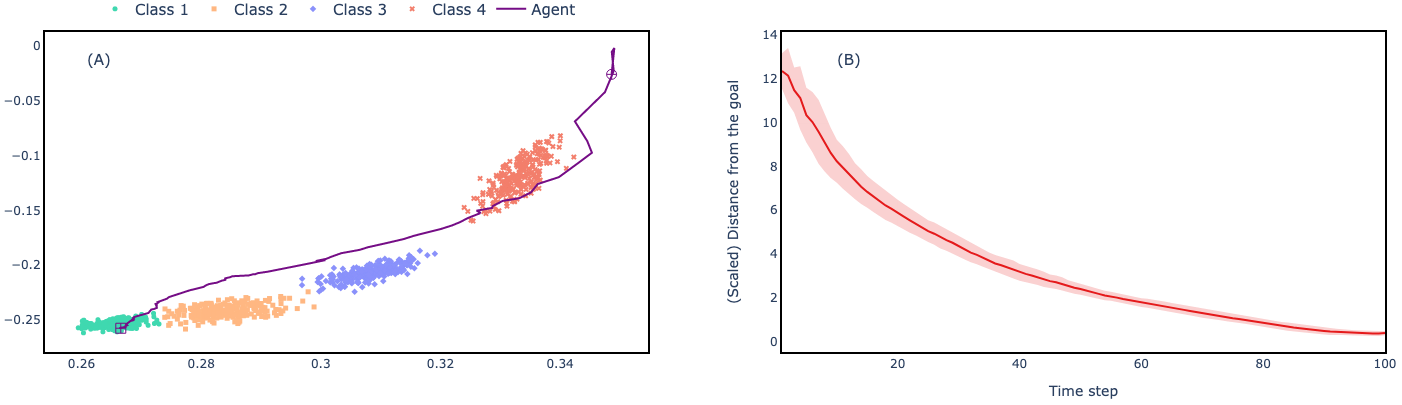
Figure 2: (A): An example of trajectory realised by the agent taken throughout a test episode. The goal for the agent is to reach the green region, i.e. the region of optimal subgraphs. The purple circle denotes the agents start position whilst the purple square denotes the agents final position. We used an autoencoder to map from the original embedding space to the 2-dimensional space in the Figure. (B): Time-series plots of how the distance from the optimal region (green in the plot on the left) changes over time. The red line is the mean distance (of 10 random episodes) per episode time step, with the shaded area corresponding to the 95% confidence interval. Here the distance is computed in the original space (i.e. without using the autoencoder for dimensionality reduction) and is scaled using $\beta$ from Equation (4)

.

4 Experimental studies

Setup

We extensively test the performance of LeNSE on the following three budget constrained problems:

Max Vertex Cover (MVC): Given a graph $G=(V,E)$ and a budget $b$, find a set $X^{*}$ of $b$ vertices such that the coverage of $X^{*}$ is maximised, i.e.

$$X^{*}=\underset{X\subset V:|X|=b}{\arg\max}f(X)\;;$$ (8)

where $f(X)=\frac{|Y|}{|E|}$ with $Y=\{(u,v)\in E:u\in X,v\in V\}$.

Budgeted Max Cut (BMC): Given a graph $G=(V,E)$ and a budget $b$, find a set $X^{*}$ of $b$ vertices such that the cut set induced by $X^{*}$ is maximised, i.e.

$$X^{*}=\underset{X\subset V:|X|=b}{\arg\max}f(X)\;;$$ (9)

where $f(X)=|\{(u,v)\in E:v\in X,u\in V\setminus X\}|$.

Influence Maximisation (IM): Given a directed weighted graph $G=(V,E)$, a budget $b$, and an information diffusion model $\mathcal{D}$, we are to select a set $X^{*}$ of $b$ vertices such that the expected spread of influence under $\mathcal{D}$ is maximised, i.e.

$$X^{*}=\underset{X\subset V:|X|=b}{\arg\max}\mathbb{E}_{\mathcal{D}}\left[f(X)\right]\;;$$

where $f(X)$ denotes the spread of a set of vertices $X$. We consider the spread of influence under the Independent Cascade diffusion model introduced by Kempe et al. (2003).

Each problem is tested using eight real-world graphs obtained from the Snap-Stanford repository (Leskovec & Krevl, 2014). For each graph, we randomly sample a percentage of the graphs’ edges to form a training graph, with testing then done on the graph formed from the held out edges; the datasets used are summarised in Appendix B. All training and test episodes start from different random initial subgraphs. In all experiments, the encoder is trained to identify optimal subgraphs using a budget of $b=100$. Network architectures and hyper-parameters are detailed in Appendix C.

For our experiments we use $K=4$ classes. The label mapping function $g(x)$ assigns label $1$ if $x\in(0.95,\infty)$ (i.e. if the subgraph is optimal), $2$ if $x\in(0.8,0.95]$, $3$ if $x\in(0.6,0.8]$ and $4$ if $x\in[0,0.6]$; this is done for all graphs with the exception of the Facebook-IM/MVC problem where we only use classes 1-3. We choose a cut-off of $0.95$ for the optimal subgraph in LeNSE to allow for some error when using stochastic solvers.

Competing methods

Graph	LeNSE			GNN-R			GNN-T			GCOMB-P
	Ratio	$P_{V}$	$P_{E}$	Ratio	$P_{V}$	$P_{E}$	Ratio	$P_{V}$	$P_{E}$	Ratio	$P_{V}$	$P_{E}$
	Max Vertex Cover
Facebook	0.968 (0.009)	7%	73%	0.998	6%	2%	0.607	87%	77%	0.927	7%	1%
Wiki	1.094 (0.000)	34%	51%	1.003	34%	5%	0.371	93%	83%	0.990	3%	3%
Deezer	0.979 (0.002)	75%	94%	0.944	75%	66%	0.768	99%	99%	0.994	13%	3%
Slashdot	0.979 (0.001)	69%	83%	0.944	66%	30%	0.410	99%	95%	1.000	2%	10%
Twitter	0.989 (0.001)	33%	78%	0.985	32%	11%	0.229	99%	99%	0.997	17%	2%
DBLP	0.990 (0.001)	90%	96%	0.812	90%	80%	0.764	99%	99%	0.999	3%	1%
YouTube	0.982 (0.002)	79%	85%	0.417	78%	75%	0.317	99%	99%	0.998	7%	3%
Skitter	0.976 (0.002)	70%	84%	0.494	70%	69%	0.424	99%	99%	0.999	10%	2%
	Budgeted Max-Cut
Facebook	0.960 (0.004)	7%	67%	0.999	8%	3%	0.873	89%	70%	0.813	95%	89%
Wiki	0.981 (0.001)	39%	63%	0.997	30%	12%	0.877	97%	96%	0.920	96%	91%
Deezer	0.975 (0.002)	74%	94%	0.990	68%	55%	0.938	94%	92%	0.850	99%	99%
Slashdot	0.990 (0.001)	62%	79%	0.998	58%	28%	0.561	99%	98%	0.632	99%	99%
Twitter	0.987 (0.001)	48%	87%	0.991	44%	25%	0.820	99%	99%	0.628	99%	99%
DBLP	0.993 (0.000)	92%	97%	0.875	92%	81%	0.656	99%	98%	0.646	99%	98%
YouTube	0.987 (0.001)	79%	84%	0.613	74%	74%	0.753	99%	99%	0.536	99%	97%
Skitter	0.974 (0.004)	71%	83%	0.502	71%	60%	0.407	99%	99%	0.427	99%	99%
	Influence Maximisation
Facebook	0.979 (0.002)	9%	70%	1.006	9%	6%	0.886	91%	88%	0.951	73%	63%
Wiki	0.960 (0.002)	51%	71%	0.964	49%	78%	0.973	96%	95%	0.969	90%	81%
Deezer	0.972 (0.003)	76%	94%	0.935	76%	86%	0.775	98%	99%	0.805	95%	97%
Slashdot	0.966 (0.003)	77%	90%	0.966	74%	71%	0.951	98%	95%	0.966	98%	93%
Twitter	0.966 (0.001)	40%	88%	0.988	26%	12%	0.921	98%	97%	0.920	98%	97%
DBLP	0.969 (0.002)	89%	96%	0.935	89%	88%	0.844	99%	98%	0.863	99%	99%
YouTube	0.971 (0.001)	75%	81%	0.918	75%	75%	0.806	94%	99%	0.933	99%	99%
Skitter	0.983 (0.002)	78%	85%	0.919	69%	58%	0.883	99%	99%	0.883	99%	99%

Table 1: Results for LeNSE, GNN-R, GNN-T and GCOMB-P. The ratio reported is the ratio from Equation (2) and $P_{V},P_{E}$ denote the percentage of vertices and edges, respectively, pruned from the graph. The results for LeNSE are averaged over 10 random initial subgraphs with the standard errors for the ratio given in the brackets.

We compare LeNSE to a GNN vertex classifier and the pruning method described in GCOMB (Manchanda et al., 2020) which we denote as GCOMB-P (see Appendix E for a more detailed overview). The GNN classifier uses the same architecture as LeNSE’s encoder except with no coarsening layers. The classifier is trained to predict the probability that a vertex is one of the $b$ solution vertices. At each epoch, we randomly sample $b$ vertices that are not solution vertices, and evaluate the loss on these sampled vertices and the $b$ sampled vertices; this avoids the loss being dominated by the non-solution vertices. Using the trained classifier, we used the predicted probabilities to rank the vertices. We choose two different thresholds using the predicted probabilities. GNN-R: assuming that the subgraph returned by LeNSE has $k$ vertices, we prune from the graph the bottom $|V|-k$ ranked vertices; GNN-T: we remove all vertices with predicted probability less than 0.5.

Experimental results

We look to assess LeNSE’s ability to prune a graph, and the quality of solution that can be found on the pruned graph. To that end, we report 2 main metrics: 1) the number of vertices/edges in the final subgraph; 2) the final ratio achieved, i.e. Equation (2). Note that when reporting Equation (2), the set $X^{*}$ found by the heuristic on the test graph is used. In Table 1 we report these metrics for LeNSE and the competing methods.

We can see that for each problem and dataset LeNSE is able to find an optimal subgraph (i.e. ratio greater than 0.95). Interestingly, we see that for Wiki-MVC the heuristic was able to find a better solution on the subgraph than it did on the original graph. Note that this is possible because the greedy heuristic used for MVC has a 60% approximation ratio, and so with less noise the heuristic is able to find a better solution than on the entire graph.

In terms of the amount of pruning done, we see that LeNSE is consistently able to prune large amounts of edges from the graphs. In most instances we also see that LeNSE prunes large portions of vertices from the graph; in particular we note that for the 3 larger graphs we are able to prune 70+% in all 3 of the problems. However, as the complexity of many heuristics rely on the number of edges as well as vertices – as is the case with IMM and the MIP formulation of BMC – pruning edges is equally important as pruning vertices for reducing the run time of heuristics.

For the competing methods, we can see that whilst GCOMB-P performs well at achieving a close-to optimal ratio for IM and MVC, it performs worse in the BMC problem. This suggests that a hand-crafted pruning method may not be as effective at generalising to multiple problems compared to one which is learnt, such as in LeNSE. Further, GCOMB-P prunes very little of the graphs in the MVC problem which is likely why the ratios are consistently close to optimal. The converse can be said for GCOMB-P in the BMC problems, where it prunes too much of the graphs and hence gives lower ratios.

The GNN-R method obtains similar ratios to LeNSE for the smaller datasets, but on the larger datasets (e.g. DBLP, YouTube, Skitter) the performance starts to degenerate, suggesting that the GNN classifier is unable to generalise when the test graph is much larger than the training graph. Further, we note that with the exception of Wiki-IM this approach never prunes as many edges as LeNSE. The GNN-T approach achieves a poor ratio across all MVC and BMC datasets due to the over-pruning of the graphs. The performance is improved somewhat in the IM problem, but it still does not achieve ratios close to that obtained by LeNSE.

Further to these results, in Figure 2 we provide a visual demonstration of the policy learnt by LeNSE for the Wiki-BMC graph. In plot (A) we provide an example trajectory taken by the agent. The agent starts in a region close to the worst class of subgraphs and sequentially makes progress by moving closer to the optimal subgraphs after each action. In plot (B) we show the (scaled) distance per episode time step of the subgraph from the goal. The distance is averaged over 10 randomly initialised episodes, and we can see that the mean distance tends towards 0 as the episode goes on, with the confidence interval becoming tighter.

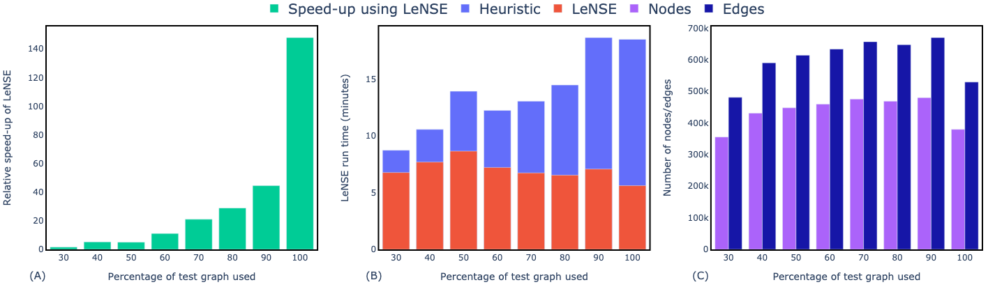
Figure 3: (A): The relative speed-up of using LeNSE vs. using the heuristic on the entire graph. (B): The time taken, in minutes, for LeNSE to run. We have broken down the run time to demonstrate the time taken for LeNSE to find a subgraph (red bars) and the time taken to run the heuristic on the subgraphs (blue bars). (C): The number of vertices/edges in the final subgraphs returned by LeNSE. In each plot we vary the percentage of the test graph used to demonstrate how the performance of LeNSE changes as the size of the graph increases. These experiments were all performed on the Talk-IM graph.

Scalability study

In Figure 3 we demonstrate the performance of LeNSE on the large Talk graph which has 2.3m vertices and 4.8m edges. In particular, we show how the performance varies as we increase the percentage of the test graph’s edges used. We report the relative speed-up of using LeNSE vs. using the heuristic on the entire graph, the run time of LeNSE and the number of vertices/edges in the subgraphs returned by LeNSE – these are all averaged over 10 random episodes. The experiments were carried out for the IM problem and we note that all the heuristic achieved a ratio greater than 0.95 on all of the subgraphs.

We can see from the Figure that despite the test graph size increasing, the time required by LeNSE to find a subgraph remains almost constant. This is due to the fact that the amount of pruning done by LeNSE increases as the size of the graph increases, and so the subgraph size passed through the encoder does not increase linearly with the size of the test graph. Importantly, we show that using LeNSE leads to more than a 140 time speed-up as opposed to using the heuristic on the full graph.

Multi-budget scores

We assess whether heuristics can also obtain (close-to) optimal results for budgets lower than that which the encoder is trained for in the pre-processing phase. As mentioned, in our experiments the encoder is trained to identify an optimal subgraph for a budget of 100. We now test whether the subgraphs returned by LeNSE can also be used to obtain an optimal score for various budgets lower than 100. Specifically, we report the ratio achieved when looking to find a solution for the following budgets: 1, 10, 25, 50 and 75.

The results for the three problems can be found in Table 4 in Appendix D. In the majority of cases the subgraphs provided by LeNSE are also optimal subgraphs for budgets lower than that which LeNSE was trained for. The exceptions are the Facebook-IM, DBLP-IM and Skitter-IM/MVC graphs for a budget of one. Despite these four instances, the evidence would suggests that a viable training option for LeNSE is to train for the largest budget that will ever be required, and it should follow that a heuristic can be used to find an optimal solution for all smaller budgets.

5 Conclusion

We have introduced LeNSE, a novel graph pruning algorithm that finds an optimal subgraph containing the solution of a CO problem. Rather than being a single algorithm, LeNSE is a general framework that can be used in combination with any existing heuristic of choice for large-scale problems. In all the settings that we have investigated using real-world graph datasets, we found that training could be done on some small percentage of the graph, being able to scale up to the held out portion of the graph without any performance degradation. We also found that the subgraphs found by LeNSE were substantially smaller than the original graph, with more than 90% of the graphs vertices and edges being removed in the best case.

Further to this, we also demonstrated that the subgraphs found by LeNSE were, in most cases, optimal subgraphs for budgets lower than that which the encoder was trained to recognise. We compared LeNSE to two baseline methods where we found that LeNSE was able to either provide a (much) better ratio than the comparisons, or prune a significant amount more of the graph whilst still finding an optimal subgraph. As well as this, LeNSE was able to consistently perform well across all problems. Finally, we demonstrated the benefits of using LeNSE on a graph with nearly $5$ million edges, showing that LeNSE achieved speed up of more than 140 times compared to not doing any pruning.

Potential avenues for future work include alternative graph modification operations, as in this work we only consider the replacement of a vertex with one of its neighbours and include all of the one-hop neighbours of some vertex subset in the subgraph. We also plan to further investigate LeNSE’s performance on other CO problems besides the budget-constrained versions presented here.

Appendix A Dataset generation

Algorithm 2 describes the procedure used to generate the dataset consisting of labelled subgraphs which are used to learn a discriminative subgraph embedding. Here, we recall that $G_{T}$ represents the train graph, and so the generated dataset will consist of subgraphs of the smaller train graph. To generate the training dataset, we sample random subgraphs and compute the corresponding label, which are assigned using a function $g(\cdot)$. We ensure a balanced dataset (i.e. an equal number of subgraphs for each one of the $K$ classes); this is achieved by ensuring that some fraction of the $b$ solution vertices, which we assume to be known on the train-graph, are present in the subgraph so that we achieve the desired score.

Algorithm 2 Dataset generation

0:  Train graph $G_{T}=(V_{T},E_{T})$, Heuristic Solver $\mathcal{H}$, Heuristic score $f(\mathcal{H}(G))$, Dataset size $N$, label mapping function $g(\cdot)$, Fixed vertex size $M$

1:  $D\leftarrow\emptyset$

2:  for $i\mbox{ in }1,2,...,N$ do

3:     $X\sim\mathcal{U}(V)$ such that $|X|=M$

4:     $S=\xi(X)$

5:     Compute ratio $r=f(\mathcal{H}(S))/f(\mathcal{H}(G))$

6:     Assign label $y=g(r)$

7:     $D\leftarrow D\cup(S,y)$

8:  end for

Appendix B Dataset information

In Table 2 we list the graphs used in our experiments and the size of the respective training and testing splits. In addition to the number of edges used for training, we also indicate what percentage of the original graphs edges were used. Note that encoder training and DQN training are all carried out on the train graph, and then tested on the held out test graph.

Graph Name	Train Size		Test Size
	Vertices	Edges	Vertices	Edges
Facebook	3,822	26,470 (30%)	3,998	61,764
Wiki	4,895	31,106 (30%)	6,349	72,583
Deezer	48,775	149,460 (30%)	53,555	348,742
Slashdot (U)	47,558	140,566 (30%)	67,677	327,988
Slashdot (D)	48,976	154,972 (30%)	68,292	361,603
Twitter (U)	55,911	134,231 (10%)	80,779	1,208,079
Twitter (D)	58,981	176,814 (10%)	80,776	1,591,335
DBLP	36,889	42,467 (04%)	314,818	1,007,399
YouTube	125,607	185,566 (06%)	1,094,439	2,802,058
Skitter	77,179	115,170 (01%)	1,694,024	10,980,128
Talk	120,443	181,843 (04%)	2,329,147	4,839,567

Table 2: The real-world graphs used to perform our experiments. For each graph, we provide the corresponding size of the training and testing sets; in brackets we indicate the percentage of edges taken from the original graph for training purposes with the remaining edges being used to form the test graph. For Slashdot and Twitter, the size of the original graph varied when we treated it as undirected/directed, so (U) refers to undirected graphs and (D) denotes the directed one. All datasets can be found at http://snap.stanford.edu/data/index.html.

Appendix C Network architectures and hyper-parameters

The encoder must be able to provide meaningful graph level embeddings, as opposed to vertex/edge embeddings. Therefore we combine convolutional layers with graph coarsening layers. The convolutional layer learns vertex features which are then used by the coarsening layer to reduce the size of the graph. Repeatedly applying such layers leads to a single vectorial representation of the input graph. In particular, our encoder architecture consists of GraphSAGE layers (Hamilton et al., 2017) to learn the vertex features and $k$-pooling layers (Cangea et al., 2018) to coarsen the graph.

Our encoder architecture has 3 layers, each one consisting of a GraphSAGE layer with ReLU activation followed immediately by a $k$-pooling layer. The output is a single vector representation of the input subgraph which is then passed through a fully connected linear layer to map to the desired dimension – the full architecture is summarised in Figure 1 of Cangea et al. (2018). For the MVC and BMC problem we use as raw vertex features the number of neighbours and the eigenvector centrality (Newman, 2008), and for the IM problem we additionally use the sum of the outgoing edge-weights of a vertex – note these are all computed relative to the original graph, not the subgraphs. Note that we normalise the number of vertices and the outgoing edge weights by min-max.

Unlike the more commonly used DQN architecture which takes in the state and outputs a Q-value for each possible action, our DQN will take in the state and action being considered and output a single Q-value. This is necessary as our action space changes at each step of an episode based on which action tuples are in $\mathcal{A}_{t}$. The DQN architecture consists of 3 independent fully connected layers where the output of each is concatenated into a single vector before being passed through 3 further linear layers. The number of hidden units in all fully connected layers is 128 and all have ReLU activations, except for the final layer which is linear as we want to map to $\mathbb{R}$ for the Q-Value. Formally, our DQN is a function $Q:\mathbb{R}^{d}\times\mathbb{R}^{d^{\prime}}\times\mathbb{R}^{d^{\prime}}\rightarrow\mathbb{R}$ where $d$ is the subgraph embedding dimensionality and $d^{\prime}$ is the dimensionality of the vertex embeddings from the first GraphSAGE layer in the encoder. We use this first GraphSAGE layer (i.e. before any pooling) to obtain vertex embeddings when passing the actions (vertices) through the DQN.

The weights of both the encoder and the DQN are optimised with the Adam optimiser (Kingma & Ba, 2014) and both have a learning rate of 0.001. The encoder batch size and experience replay batch size are both 128. We use a pooling ratio of $k=0.8$ and temperature hyper-parameter of $\tau=0.1$ in the encoder. Finally, when training the DQN we initialise the exploration parameter $\epsilon$ to be equal to one and decay it after each random action at a rate of 0.9995 down to a minimum value of 0.01. We also have a max replay memory size of 25,000, a discount factor of 0.995 and a target network which is updated after each experience replay update using polyak averaging with a parameter of 0.0025. Note that during training we use a different episode length than at test time, both of which we report, along with the remaining hyper-parameters that vary per dataset, in Table 3. Note that we only report parameters for the Talk-IM graph as we do not perform any experiments using the Talk-BMC/MVC graphs.

Graph	$M$	$n$	$d^{\prime}$	$d$	$T_{train}$	$N^{\prime}$	$\alpha$	$c$	$\beta$	$T_{test}$
	MVC
Facebook	300	100	30	10	2,000	10	0	20	50	2,000
Wiki	300	100	75	25	2,000	10	0.1	20	3	300
Deezer	500	200	50	10	2,000	10	0	20	15	300
Slashdot	500	200	30	15	2,000	10	0.1	20	20	300
Twitter	1,000	100	40	10	1,500	10	0.1	2	20	750
DBLP	1,000	100	40	10	1,500	10	0.1	2	20	1,000
Youtube	1,250	100	75	25	1,500	10	0.1	2	30	500
Skitter	750	250	75	20	1,000	10	0.05	2	30	500
	Budgeted Max-Cut
Facebook	300	250	40	10	2,000	10	0.05	20	20	2,000
Wiki	300	250	30	10	2,000	10	0.05	20	25	100
Deezer	500	250	30	10	2,000	10	0.05	20	50	300
Slashdot	500	250	30	15	2,000	10	0.05	20	50	300
Twitter	1,000	100	40	10	2,000	10	0.5	2	20	250
DBLP	1,000	100	30	10	2,000	10	0.5	2	50	1,000
Youtube	1,000	200	75	25	1,500	10	0.5	2	5	400
Skitter	750	500	75	25	1,000	10	0.05	2	30	500
	Influence Maximisation
Facebook	300	100	30	10	5,000	10	0	20	50	5,000
Wiki	300	100	50	15	2,000	10	0	20	50	200
Deezer	500	100	30	10	2,000	10	0	20	15	1,500
Slashdot	500	100	50	10	2,000	10	0	20	15	300
Twitter	1,000	100	40	10	1,500	10	0.5	2	20	400
DBLP	1,000	100	40	10	1,500	10	0.5	2	20	1,000
Youtube	750	100	75	25	1,500	10	0.1	2	20	500
Skitter	750	250	75	20	500	25	0.05	2	10	500
Talk	750	400	75	25	500	25	0.1	2	10	100

Table 3: The hyperparameters used when training LeNSE. $M$ denotes the size of the vertex subset we use to induce the subgraphs throughout training, $n$ denotes the number of samples per class in the subgraph dataset, $N^{\prime}$ is the number of training episodes, $d^{\prime}$ corresponds to the dimensionality of the vertex embeddings for the GraphSAGE layers in the encoder whilst $d$ is the final embedding dimension of the encoder, $c$ denotes the frequency with which we perform SGD on the parameters of the DQN as per Algorithm 1, $\beta$ is the scaling factor in the rewards and $T_{train},T_{test}$ denote the length of the train and test episodes, respectively.

Appendix D Multi budget test results

Table 4 contains the results for the multi budget test results referenced in the main paper. We can see that all the ratios, except for Facebook-IM, DBLP-IM and Skitter-MVC/IM, are ratios we would expect from an optimal subgraph. In particular, the ratios for the deterministic solvers in MVC and BMC are all close to 1.

Graph	Budget
	1	10	25	50	75	100
	Max Vertex Cover
Facebook	1.00	1.00	0.99	0.97	0.97	0.97
Wiki	1.00	1.00	1.00	1.00	1.04	1.09
Deezer	1.00	1.00	1.00	0.99	0.99	0.98
Slashdot	1.00	1.00	1.00	1.00	0.99	0.98
Twitter	1.00	1.00	1.00	1.00	1.00	0.99
DBLP	1.00	1.00	1.00	1.00	0.99	0.99
YouTube	1.00	1.00	1.00	1.00	0.99	0.98
Skitter	0.85	0.98	0.99	0.99	0.99	0.98
	Budgeted Max-Cut
Facebook	1.00	1.00	0.99	0.98	0.98	0.96
Wiki	1.00	1.00	1.00	1.00	1.00	0.98
Deezer	1.00	1.00	1.00	0.99	0.99	0.98
Slashdot	1.00	1.00	1.00	1.00	1.00	0.99
Twitter	0.98	1.00	1.00	1.00	0.99	0.99
DBLP	1.00	1.00	1.00	1.00	1.00	0.99
YouTube	1.00	1.00	1.00	1.00	0.99	0.99
Skitter	0.96	1.00	1.00	0.99	0.99	0.97
	Influence Maximisation
Facebook	0.86	0.99	0.98	0.99	0.99	0.98
Wiki	1.00	0.98	0.99	1.00	0.98	0.96
Deezer	1.00	0.97	0.97	0.97	0.97	0.97
Slashdot	1.00	0.99	0.99	0.98	0.98	0.98
Twitter	1.00	0.97	0.96	0.96	0.96	0.96
DBLP	0.86	0.96	0.95	0.97	0.96	0.97
YouTube	1.00	0.96	0.98	0.98	0.97	0.97
Skitter	0.77	0.97	0.98	0.98	0.98	0.98

Table 4: Results showing the ratio achieved for the three CO problems, averaged over 10 runs, for budgets lower than that which the encoder was trained to attain.

Appendix E GCOMB-based graph pruning

The methodology presented in Manchanda et al. (2020) can be broken down into two parts – a pruning phase and a Q-learning phase. The pruning is based on a vertex ranking approach. For a train graph $G=(V,E)$ and budget of $b$, the vertices are initially sorted into descending order based on the outgoing edge-weight (or degree in an unweighted graph) and $rank(v)$ denotes the position of vertex $v$ in this ordered list. A stochastic solver is used $L$ times to obtain $L$ (different) solution sets $\{A^{(i)}\}_{i=1}^{L}$ of size $b$. If we define $A^{(i)}_{:k}$ to be the first $k$ vertices added to solution set $A^{(i)}$, then for all budgets $b^{\prime}\leq b$ we define $r_{b^{\prime}}=\max_{v\in\cup_{i}A^{(i)}_{:k}}rank(v)$ to be the highest rank of all vertices amongst the first $b^{\prime}$ vertices in each of the $L$ solution sets. A linear interpolator is then used to fit these $(b^{\prime},r_{b^{\prime}})$ pairs. Now, for a budget $\tilde{b}$, the test graph is pruned by using the linear interpolator to predict a rank $\hat{r}_{\tilde{b}}$ and remove all vertices in the test graph with rank greater than $\hat{r}_{\tilde{b}}$, where the rankings of the test graph and calculated in the same way as for the train graph. Note that when training the linear interpolator the rankings and budgets are normalised by the proportion of vertices in the graph to enable generalisation to different graphs. In our experiments, the stochastic solvers that we use for the 3 problems are IMM (Tang et al., 2015) for IM, the heuristic introduced in Hassin & Rubinstein (2000) for BMC and for MVC we use the probabilistic-greedy that was introduced in the GCOMB paper. For the Q-learning phase of GCOMB, a simple Q-learning algorithm is deployed on the pruned graph. This is in contrast to LeNSE, where we use an existing heuristic.

Appendix F Loss Comparisons

Graph	Loss
	InfoNCE	Cross-Entropy	Ordinal
	Max Vertex Cover
Facebook	0.968	0.907	0.880
Wiki	1.094	0.899	0.931
	Budgeted Max-Cut
Facebook	0.960	0.647	0.650
Wiki	0.981	0.391	0.603
	Influence Maximisation
Facebook	0.979	0.663	0.871
Wiki	0.960	0.895	0.914

Table 5: Comparison of the average ratios from Equation (2) achieved when using the different loss functions.

We compare the InfoNCE loss to the standard cross entropy loss as well as to an ordinal classification based loss. We choose to compare to an ordinal based loss function as there is an ordinal structure to the classes. For example, it would be more acceptable to misclassify a class 4 subgraph as a class 3 subgraph than it would be to classify it as a class 1 subgraph. We choose the ordinal classification approach introduced in Cheng et al. (2008). With $K$ classes, a subgraph with class $i\leq K$ is assigned an ordinal target vector $y$ where $y_{j}=1$ for $j\leq i$, and 0 otherwise. The output layer uses a sigmoid activation so that the predicted vector $\hat{y}$ has individual values in the range $(0,1)$ and the network is trained to minimise the mean squared error between the $\hat{y}$ and $y$. To make the comparisons fair we use the same encoder (i.e. same architecture) for each loss function, where the ordinal and cross entropy have the additional layer to map from the embedding space to the prediction vector as required.

In Figure 4 we present example embeddings using the 3 different loss functions for the Wiki-BMC graph, and in Table 5 we present the corresponding average ratios obtained by LeNSE when using embeddings trained with the respective losses. We can see from the table that the variation is much higher when using cross entropy and ordinal trained encoders. This is likely due to what we see in Figure 4 where the embeddings provided are not as well separated as when using the InfoNCE loss. In particular, the cross entropy embeddings have no clear structure, with class 3 and 4 subgraphs being embedded in the same location as class 1 and 2 (hence why they cannot be seen on the Figure) – this is likely the cause for LeNSE achieving a ratio of just 0.391. Interestingly, the ordinal embeddings in the Figure highlight why the InfoNCE loss is useful as we can see that for class 1 there are two separate clusters, including some overlap with class 2. This highlights why uni-modality is useful as LeNSE obtained a ratio of only 0.603 using this embedding. This can be explained by the fact that the goal would have been at the centre of the two clusters which does not necessarily correspond to a good region of the embedding. In contrast to this, we see in Figure 5 that all the embeddings provided by the InfoNCE loss have uni-modal clusterings with the monotonic ordering of the classes maintained, with an exception in the Twitter-BMC graph where classes 3 and 4 are well separated but are approximately a similar distance from the class 1 embeddings.

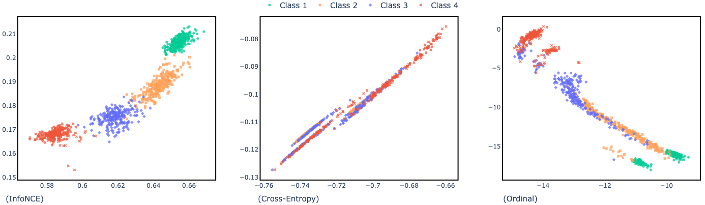
Figure 4: Example of the embeddings provided for the Wiki-BMC graph by the InfoNCE loss, cross entropy loss and ordinal loss. Note that autoencoders were used for dimensionality reduction to map from the original embedding space to the plotted 2-dimensional space.

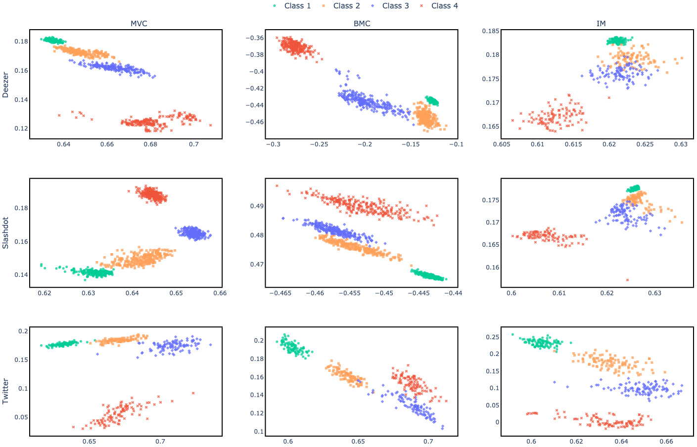
Figure 5: Example of embeddings provided by the InfoNCE loss for various graph/problem combinations. Note that autoencoders were used for dimensionality reduction to map from the original embedding space to the plotted 2-dimensional space.

References

- Almasan et al. (2019) Almasan, P., Suárez-Varela, J., Badia-Sampera, A., Rusek, K., Barlet-Ros, P., and Cabellos-Aparicio, A. Deep reinforcement learning meets graph neural networks: Exploring a routing optimization use case. arXiv preprint arXiv:1910.07421, 2019.
- Amanatidis et al. (2017) Amanatidis, G., Birmpas, G., and Markakis, E. On budget-feasible mechanism design for symmetric submodular objectives. In International Conference on Web and Internet Economics, pp. 1–15. Springer, 2017.
- Applegate et al. (2001) Applegate, D., Bixby, R., Chvátal, V., and Cook, W. Tsp cuts which do not conform to the template paradigm. In Computational combinatorial optimization, pp. 261–303. Springer, 2001.
- Arora et al. (2017) Arora, A., Galhotra, S., and Ranu, S. Debunking the myths of influence maximization: An in-depth benchmarking study. In Proceedings of the 2017 ACM international conference on management of data, pp. 651–666, 2017.
- Arumugam et al. (2016) Arumugam, S., Brandstädt, A., Nishizeki, T., and Thulasiraman, K. Handbook of graph theory, combinatorial optimization, and algorithms, volume 34. CRC Press, 2016.
- Ausiello et al. (2012) Ausiello, G., Crescenzi, P., Gambosi, G., Kann, V., Marchetti-Spaccamela, A., and Protasi, M. Complexity and approximation: Combinatorial optimization problems and their approximability properties. Springer Science & Business Media, 2012.
- Avis et al. (2005) Avis, D., Hertz, A., and Marcotte, O. Graph theory and combinatorial optimization, volume 8. Springer Science & Business Media, 2005.
- Bai et al. (2021) Bai, Y., Xu, D., Sun, Y., and Wang, W. Glsearch: Maximum common subgraph detection via learning to search. In International Conference on Machine Learning, pp. 588–598. PMLR, 2021.
- Barahona et al. (1988) Barahona, F., Grötschel, M., Jünger, M., and Reinelt, G. An application of combinatorial optimization to statistical physics and circuit layout design. Operations Research, 36(3):493–513, 1988.
- Barrett et al. (2020) Barrett, T., Clements, W., Foerster, J., and Lvovsky, A. Exploratory combinatorial optimization with reinforcement learning. In Proceedings of the AAAI Conference on Artificial Intelligence, volume 34, pp. 3243–3250, 2020.
- Battaglia et al. (2018) Battaglia, P. W., Hamrick, J. B., Bapst, V., Sanchez-Gonzalez, A., Zambaldi, V., Malinowski, M., Tacchetti, A., Raposo, D., Santoro, A., Faulkner, R., et al. Relational inductive biases, deep learning, and graph networks. arXiv preprint arXiv:1806.01261, 2018.
- Bellman (1957) Bellman, R. A markovian decision process. Journal of mathematics and mechanics, 6(5):679–684, 1957.
- Bello et al. (2016) Bello, I., Pham, H., Le, Q. V., Norouzi, M., and Bengio, S. Neural combinatorial optimization with reinforcement learning. arXiv preprint arXiv:1611.09940, 2016.
- Bengio et al. (2020) Bengio, Y., Lodi, A., and Prouvost, A. Machine learning for combinatorial optimization: a methodological tour d’horizon. European Journal of Operational Research, 2020.
- Borgs et al. (2014) Borgs, C., Brautbar, M., Chayes, J., and Lucier, B. Maximizing social influence in nearly optimal time. In Proceedings of the twenty-fifth annual ACM-SIAM symposium on Discrete algorithms, pp. 946–957. SIAM, 2014.
- Brody et al. (2021) Brody, S., Alon, U., and Yahav, E. How attentive are graph attention networks? arXiv preprint arXiv:2105.14491, 2021.
- Bronstein et al. (2017) Bronstein, M. M., Bruna, J., LeCun, Y., Szlam, A., and Vandergheynst, P. Geometric deep learning: going beyond euclidean data. IEEE Signal Processing Magazine, 34(4):18–42, 2017.
- Brown & Reingen (1987) Brown, J. J. and Reingen, P. H. Social ties and word-of-mouth referral behavior. Journal of Consumer research, 14(3):350–362, 1987.
- Cangea et al. (2018) Cangea, C., Veličković, P., Jovanović, N., Kipf, T., and Liò, P. Towards sparse hierarchical graph classifiers. arXiv preprint arXiv:1811.01287, 2018.
- Chaoji et al. (2012) Chaoji, V., Ranu, S., Rastogi, R., and Bhatt, R. Recommendations to boost content spread in social networks. In Proceedings of the 21st international conference on World Wide Web, pp. 529–538, 2012.
- Chen et al. (2020) Chen, T., Kornblith, S., Norouzi, M., and Hinton, G. A simple framework for contrastive learning of visual representations. In International conference on machine learning, pp. 1597–1607. PMLR, 2020.
- Chen et al. (2010) Chen, W., Wang, C., and Wang, Y. Scalable influence maximization for prevalent viral marketing in large-scale social networks. In Proceedings of the 16th ACM SIGKDD international conference on Knowledge discovery and data mining, pp. 1029–1038, 2010.
- Cheng et al. (2008) Cheng, J., Wang, Z., and Pollastri, G. A neural network approach to ordinal regression. In 2008 IEEE international joint conference on neural networks (IEEE world congress on computational intelligence), pp. 1279–1284. IEEE, 2008.
- Cheng et al. (2013) Cheng, S., Shen, H., Huang, J., Zhang, G., and Cheng, X. Staticgreedy: solving the scalability-accuracy dilemma in influence maximization. In Proceedings of the 22nd ACM international conference on Information & Knowledge Management, pp. 509–518, 2013.
- Cheng et al. (2014) Cheng, S., Shen, H., Huang, J., Chen, W., and Cheng, X. Imrank: influence maximization via finding self-consistent ranking. In Proceedings of the 37th international ACM SIGIR conference on Research & development in information retrieval, pp. 475–484, 2014.
- Cohen et al. (2014) Cohen, E., Delling, D., Pajor, T., and Werneck, R. F. Sketch-based influence maximization and computation: Scaling up with guarantees. In Proceedings of the 23rd ACM International Conference on Conference on Information and Knowledge Management, pp. 629–638, 2014.
- Dai et al. (2016) Dai, H., Dai, B., and Song, L. Discriminative embeddings of latent variable models for structured data. In International conference on machine learning, pp. 2702–2711. PMLR, 2016.
- Dai et al. (2017) Dai, H., Khalil, E. B., Zhang, Y., Dilkina, B., and Song, L. Learning combinatorial optimization algorithms over graphs. arXiv preprint arXiv:1704.01665, 2017.
- Dinur & Safra (2005) Dinur, I. and Safra, S. On the hardness of approximating minimum vertex cover. Annals of mathematics, pp. 439–485, 2005.
- Dobzinski et al. (2011) Dobzinski, S., Papadimitriou, C. H., and Singer, Y. Mechanisms for complement-free procurement. In Proceedings of the 12th ACM conference on Electronic commerce, pp. 273–282, 2011.
- Gasse et al. (2019) Gasse, M., Chételat, D., Ferroni, N., Charlin, L., and Lodi, A. Exact combinatorial optimization with graph convolutional neural networks. arXiv preprint arXiv:1906.01629, 2019.
- Gilmer et al. (2017) Gilmer, J., Schoenholz, S. S., Riley, P. F., Vinyals, O., and Dahl, G. E. Neural message passing for quantum chemistry. In International conference on machine learning, pp. 1263–1272. PMLR, 2017.
- Goemans & Williamson (1995) Goemans, M. X. and Williamson, D. P. Improved approximation algorithms for maximum cut and satisfiability problems using semidefinite programming. Journal of the ACM (JACM), 42(6):1115–1145, 1995.
- Goyal et al. (2011) Goyal, A., Bonchi, F., and Lakshmanan, L. V. A data-based approach to social influence maximization. arXiv preprint arXiv:1109.6886, 2011.
- Grassia et al. (2019) Grassia, M., Lauri, J., Dutta, S., and Ajwani, D. Learning multi-stage sparsification for maximum clique enumeration. arXiv preprint arXiv:1910.00517, 2019.
- Grötschel et al. (2012) Grötschel, M., Lovász, L., and Schrijver, A. Geometric algorithms and combinatorial optimization, volume 2. Springer Science & Business Media, 2012.
- Hamilton et al. (2017) Hamilton, W. L., Ying, R., and Leskovec, J. Inductive representation learning on large graphs. arXiv preprint arXiv:1706.02216, 2017.
- Hassin & Rubinstein (2000) Hassin, R. and Rubinstein, S. Approximation algorithms for maximum linear arrangement. In Scandinavian Workshop on Algorithm Theory, pp. 231–236. Springer, 2000.
- He et al. (2020) He, K., Fan, H., Wu, Y., Xie, S., and Girshick, R. Momentum contrast for unsupervised visual representation learning. In Proceedings of the IEEE/CVF Conference on Computer Vision and Pattern Recognition, pp. 9729–9738, 2020.
- Hochbaum (1982) Hochbaum, D. S. Approximation algorithms for the set covering and vertex cover problems. SIAM Journal on computing, 11(3):555–556, 1982.
- Joshi et al. (2019) Joshi, C. K., Laurent, T., and Bresson, X. An efficient graph convolutional network technique for the travelling salesman problem. arXiv preprint arXiv:1906.01227, 2019.
- Karakostas (2005) Karakostas, G. A better approximation ratio for the vertex cover problem. In International Colloquium on Automata, Languages, and Programming, pp. 1043–1050. Springer, 2005.
- Karp (1972) Karp, R. M. Reducibility among combinatorial problems. In Complexity of computer computations, pp. 85–103. Springer, 1972.
- Kempe et al. (2003) Kempe, D., Kleinberg, J., and Tardos, É. Maximizing the spread of influence through a social network. In Proceedings of the ninth ACM SIGKDD international conference on Knowledge discovery and data mining, pp. 137–146, 2003.
- Kempe et al. (2010) Kempe, D., Salek, M., and Moore, C. Frugal and truthful auctions for vertex covers, flows and cuts. In 2010 IEEE 51st Annual Symposium on Foundations of Computer Science, pp. 745–754. IEEE, 2010.
- Khalil et al. (2016) Khalil, E., Le Bodic, P., Song, L., Nemhauser, G., and Dilkina, B. Learning to branch in mixed integer programming. In Proceedings of the AAAI Conference on Artificial Intelligence, volume 30, 2016.
- Kingma & Ba (2014) Kingma, D. P. and Ba, J. Adam: A method for stochastic optimization. arXiv preprint arXiv:1412.6980, 2014.
- Kipf & Welling (2016) Kipf, T. N. and Welling, M. Semi-supervised classification with graph convolutional networks. arXiv preprint arXiv:1609.02907, 2016.
- Kool et al. (2018) Kool, W., Van Hoof, H., and Welling, M. Attention, learn to solve routing problems! arXiv preprint arXiv:1803.08475, 2018.
- Korte et al. (2011) Korte, B. H., Vygen, J., Korte, B., and Vygen, J. Combinatorial optimization, volume 1. Springer, 2011.
- Laterre et al. (2018) Laterre, A., Fu, Y., Jabri, M. K., Cohen, A.-S., Kas, D., Hajjar, K., Dahl, T. S., Kerkeni, A., and Beguir, K. Ranked reward: Enabling self-play reinforcement learning for combinatorial optimization. arXiv preprint arXiv:1807.01672, 2018.
- Lauri et al. (2020) Lauri, J., Dutta, S., Grassia, M., and Ajwani, D. Learning fine-grained search space pruning and heuristics for combinatorial optimization. arXiv preprint arXiv:2001.01230, 2020.
- Lee et al. (2019) Lee, J., Lee, I., and Kang, J. Self-attention graph pooling. In International Conference on Machine Learning, pp. 3734–3743. PMLR, 2019.
- Leskovec & Krevl (2014) Leskovec, J. and Krevl, A. SNAP Datasets: Stanford large network dataset collection. http://snap.stanford.edu/data, June 2014.
- Li et al. (2019) Li, H., Xu, M., Bhowmick, S. S., Sun, C., Jiang, Z., and Cui, J. Disco: influence maximization meets network embedding and deep learning. arXiv preprint arXiv:1906.07378, 2019.
- Liang et al. (2020) Liang, Y., Zhang, Y., Gao, D., and Xu, Q. Mxpool: Multiplex pooling for hierarchical graph representation learning. arXiv preprint arXiv:2004.06846, 2020.
- Liu et al. (2021) Liu, D., Lodi, A., and Tanneau, M. Learning chordal extensions. Journal of Global Optimization, pp. 1–20, 2021.
- Ma et al. (2019) Ma, Q., Ge, S., He, D., Thaker, D., and Drori, I. Combinatorial optimization by graph pointer networks and hierarchical reinforcement learning. arXiv preprint arXiv:1911.04936, 2019.
- Manchanda et al. (2020) Manchanda, S., MITTAL, A., Dhawan, A., Medya, S., Ranu, S., and Singh, A. Gcomb: Learning budget-constrained combinatorial algorithms over billion-sized graphs. In Larochelle, H., Ranzato, M., Hadsell, R., Balcan, M. F., and Lin, H. (eds.), Advances in Neural Information Processing Systems, volume 33, pp. 20000–20011. Curran Associates, Inc., 2020. URL https://proceedings.neurips.cc/paper/2020/file/e7532dbeff7ef901f2e70daacb3f452d-Paper.pdf.
- Mazyavkina et al. (2021) Mazyavkina, N., Sviridov, S., Ivanov, S., and Burnaev, E. Reinforcement learning for combinatorial optimization: A survey. Computers & Operations Research, pp. 105400, 2021.
- Mnih et al. (2015) Mnih, V., Kavukcuoglu, K., Silver, D., Rusu, A. A., Veness, J., Bellemare, M. G., Graves, A., Riedmiller, M., Fidjeland, A. K., Ostrovski, G., et al. Human-level control through deep reinforcement learning. nature, 518(7540):529–533, 2015.
- Newman (2008) Newman, M. E. The mathematics of networks. The new palgrave encyclopedia of economics, 2(2008):1–12, 2008.
- Oord et al. (2018) Oord, A. v. d., Li, Y., and Vinyals, O. Representation learning with contrastive predictive coding. arXiv preprint arXiv:1807.03748, 2018.
- Reis et al. (2019) Reis, A. C., Halper, S. M., Vezeau, G. E., Cetnar, D. P., Hossain, A., Clauer, P. R., and Salis, H. M. Simultaneous repression of multiple bacterial genes using nonrepetitive extra-long sgrna arrays. Nature biotechnology, 37(11):1294–1301, 2019.
- Rogers (2010) Rogers, E. M. Diffusion of innovations. Simon and Schuster, 2010.
- Song & Ermon (2020) Song, J. and Ermon, S. Multi-label contrastive predictive coding. arXiv preprint arXiv:2007.09852, 2020.
- Sun et al. (2019) Sun, Y., Li, X., and Ernst, A. Using statistical measures and machine learning for graph reduction to solve maximum weight clique problems. IEEE transactions on pattern analysis and machine intelligence, 2019.
- Sun et al. (2021) Sun, Y., Ernst, A., Li, X., and Weiner, J. Generalization of machine learning for problem reduction: a case study on travelling salesman problems. OR Spectrum, 43(3):607–633, 2021.
- Tang et al. (2014) Tang, Y., Xiao, X., and Shi, Y. Influence maximization: Near-optimal time complexity meets practical efficiency. In Proceedings of the 2014 ACM SIGMOD international conference on Management of data, pp. 75–86, 2014.
- Tang et al. (2015) Tang, Y., Shi, Y., and Xiao, X. Influence maximization in near-linear time: A martingale approach. In Proceedings of the 2015 ACM SIGMOD International Conference on Management of Data, pp. 1539–1554, 2015.
- Valente (1996) Valente, T. W. Social network thresholds in the diffusion of innovations. Social networks, 18(1):69–89, 1996.
- Veličković et al. (2017) Veličković, P., Cucurull, G., Casanova, A., Romero, A., Lio, P., and Bengio, Y. Graph attention networks. arXiv preprint arXiv:1710.10903, 2017.
- Veličković et al. (2018) Veličković, P., Fedus, W., Hamilton, W. L., Liò, P., Bengio, Y., and Hjelm, R. D. Deep graph infomax. arXiv preprint arXiv:1809.10341, 2018.
- Vesselinova et al. (2020) Vesselinova, N., Steinert, R., Perez-Ramirez, D. F., and Boman, M. Learning combinatorial optimization on graphs: A survey with applications to networking. IEEE Access, 8:120388–120416, 2020.
- Vinyals et al. (2015) Vinyals, O., Fortunato, M., and Jaitly, N. Pointer networks. arXiv preprint arXiv:1506.03134, 2015.
- Wang et al. (2021) Wang, R., Hua, Z., Liu, G., Zhang, J., Yan, J., Qi, F., Yang, S., Zhou, J., and Yang, X. A bi-level framework for learning to solve combinatorial optimization on graphs. arXiv preprint arXiv:2106.04927, 2021.
- Watkins & Dayan (1992) Watkins, C. J. and Dayan, P. Q-learning. Machine learning, 8(3-4):279–292, 1992.
- Wilder et al. (2018) Wilder, B., Ou, H.-C., de la Haye, K., and Tambe, M. Optimizing network structure for preventative health. In AAMAS, pp. 841–849, 2018.
- Wolsey & Nemhauser (1999) Wolsey, L. A. and Nemhauser, G. L. Integer and combinatorial optimization, volume 55. John Wiley & Sons, 1999.
- Wu et al. (2020) Wu, Z., Pan, S., Chen, F., Long, G., Zhang, C., and Philip, S. Y. A comprehensive survey on graph neural networks. IEEE transactions on neural networks and learning systems, 32(1):4–24, 2020.
- Yao et al. (2021) Yao, F., Cai, R., and Wang, H. Reversible action design for combinatorial optimization with reinforcement learning. arXiv preprint arXiv:2102.07210, 2021.
- Ying et al. (2018) Ying, R., You, J., Morris, C., Ren, X., Hamilton, W. L., and Leskovec, J. Hierarchical graph representation learning with differentiable pooling. arXiv preprint arXiv:1806.08804, 2018.
- Zhou et al. (2020) Zhou, J., Cui, G., Hu, S., Zhang, Z., Yang, C., Liu, Z., Wang, L., Li, C., and Sun, M. Graph neural networks: A review of methods and applications. AI Open, 1:57–81, 2020.